Convergence of Implicit Difference Scheme for 1D Lagrangian Hydrodynamics coupled to Radiation Transport Equation

Abstract

A fully implicit finite difference scheme has been developed to solve the hydrodynamic equations coupled with radiation transport. Solution of the time dependent radiation transport equation is obtained using the discrete ordinates method and the energy flow into the Lagrangian meshes as a result of radiation interaction is fully accounted for. A tridiagonal matrix system is solved at each time step to determine the hydrodynamic variables implicitly. The results obtained from this fully implicit radiation hydrodynamics code in the planar geometry agrees well with the scaling law for radiation driven strong shock propagation in aluminium. For the point explosion problem the self similar solutions are compared with results for pure hydrodynamic case in spherical geometry and the effect of radiation energy transfer is determined. Having, thus, benchmarked the code, convergence of the method w.r.t. time step is studied in detail and compared with the results of commonly used semi-implicit method. It is shown that significant error reduction is feasible in the implicit method in comparison to the semi-implicit method, though at the cost of slightly more CPU time.

Keywords: Implicit radiation hydrodynamics, Lagrangian meshes, finite difference scheme, point explosion problem, self similar solutions

PACS: 47.11.-j, 47.11.Bc, 47.40.-x

1 Introduction

Radiation transport and its interaction with matter via emission, absorption and scattering of radiation have a substantial effect on both the state and the motion of materials in high temperature hydrodynamic flows occurring in inertial confinement fusion (ICF), strong explosions and astrophysical systems [1]. For many applications the dynamics can be considered non-relativistic since the flow velocities are much less than the speed of light. In order to describe properly the dynamics of the radiating flow, it is necessary to solve the full time-dependent radiation transport equation as very short time scales ($t_{R}\sim l/c\ \mbox{or}\ t_{\lambda}\sim\lambda_{p}/c$ corresponding to a photon flight time over a characteristic structural length $l$, or over a photon mean free path $\lambda_{p}$ ) are to be considered [2].Two methods commonly used are non-equilibrium diffusion theory [4], [3] and radiation heat conduction approximation [1]. The former is valid for optically thick bodies, where the density gradients are small and the angular distribution of photons is nearly isotropic. The conduction approximation is only applicable when matter and radiation are in local thermodynamic equilibrium, so that the radiant energy flux is proportional to temperature gradient, and for slower hydrodynamics time scales [1]. Use of Eddington’s factor for closing the first two moment equations is yet another approach followed in radiation hydrodynamics [5]. Radiative phenomena occur on time scales that differ by many orders of magnitude from those characterizing hydrodynamic flow. This leads to significant computational challenges in the efficient modeling of radiation hydrodynamics.

In this paper we solve the equations of hydrodynamics and the time dependent radiation transport equation fully implicitly. The anisotropy in the angular distribution of photons is treated in a direct way using the discrete ordinates method. Finite difference analysis is used for the Lagrangian meshes to obtain the thermodynamic variables. The hydrodynamic evolution of the system is considered in a fully implicit manner by solving a tridiagonal system of equations to obtain the velocities. The pressures and temperatures are converged iteratively.

Earlier studies on the non-equilibrium radiation diffusion calculations show that the accuracy of the solution increases on converging the non-linearities within a time step and increasing benefit is obtained as the problem becomes more and more nonlinear and faster [6], [7]. In this work, by iteratively converging the thermodynamic variables, we observe a faster decrease in the $L_{2}$-Error as compared to the commonly used semi-implicit scheme.

The organization of the paper is as follows: In section 2 we discuss the finite difference scheme for solving the hydrodynamic equations followed by the solution procedure of the radiation transport equation and their coupling together to result in an implicit radiation hydrodynamics code. Section 3 presents the results obtained using this fully implicit one-dimensional radiation hydrodynamics code for the problems of shock propagation in aluminium and the point explosion problem. These benchmark results, thus, prove the validity of the methods. Next, extensive results of convergence studies w.r.t. time step are presented. These results using the full transport equation are new, though similar studies have been reported earlier within approximate methods [3], [8]. Finally the conclusions of this paper are presented in section 4.

2 Simulation model

2.1 Implicit finite difference scheme for solving the hydrodynamic equations using a Lagrangian grid.

2.1.1 Grid structure

For hydrodynamics calculations, the medium is divided into a number of cells as shown in Fig. 1. The coordinate of the $i$ th vertex is denoted by $r_{i}$ and the region between the $(i-1)$ and $i$ th vertices is the $i$ th cell. The density of the $i$ th grid is $\rho_{i}$ and its mass is given by

$$m_{i}=\acute{c}\times\rho_{i}\times(r_{i}^{\delta}-r_{i-1}^{\delta})$$ (1)

with $\acute{c}=1,\pi,(4/3)\times\pi$ and $\delta=1,2,3$ for planar, cylindrical and spherical geometries respectively. Velocity of the $i$ th vertex is denoted by $u_{i}$ and $P_{i},V_{i},T_{ion,i},T_{elec,i},E_{ion,i}$ and $E_{elec,i}$ are the total pressure, specific volume, temperature of ions and electrons and the specific internal energy of ions and electrons in the $i$ th mesh respectively.

2.1.2 Lagrangian step

During a time interval $\Delta t\$the vertexes $r_{i}$ of the cells move as

$$\tilde{r}_{i}=r_{i}+u_{i}^{\star}\Delta t$$ (2)

$$u_{i}^{\star}=(1/2)(u_{i}+\tilde{u}_{i})$$ (3)

where $u_{i}^{\star}$ is the average of velocity values at the beginning and end of the Lagrangian step, $u_{i}$ and $\tilde{u}_{i}$ , respectively.

2.1.3 Discretized form of the hydrodynamic equations

In the Lagrangian formulation of hydrodynamics, the mass of each cell remains constant thereby enforcing mass conservation.

The Lagrangian differential equation for the conservation of momentum is

$$\rho\frac{d\vec{u}}{dt}=-\vec{\nabla}P$$ (4)

Here, the total pressure is the sum of the electron, ion and radiation pressures i.e. $P=P_{ion}+P_{elec}+P_{rad}$. Eq. [4] can be discretized for the velocity $\tilde{u}_{i}$ at the end of the time step in terms of the pressures, $P_{i}^{1/2}\mbox{and}\ P_{i+1}^{1/2}$ in the $i$ th and $i+1$ th meshes respectively, after half time step as [9]

$$\tilde{u}_{i}=u_{i}-\frac{(P_{i+1}^{1/2}-P_{i}^{1/2})\Delta t}{\rho_{i+1}(r_{i+1/2}-r_{i})+\rho_{i}(r_{i}-r_{i-1/2})}$$ (5)

The velocity in the $i$ th mesh $\tilde{u}_{i}$ is determined by the pressure in the $i$ th and $i+1$ th meshes and hence all the meshes are connected. Mass conservation equation can be used to eliminate the pressures at half time step to obtain an equation relating the present time step velocities in the adjacent meshes as follows:

The equation describing conservation of mass is

$$\frac{d\rho}{dt}=-\rho(\vec{\nabla}.\vec{u})$$ (6)

where $\rho$ is the mass density of the medium. This equation can be rewritten in terms of pressure using the relation, $\frac{dP}{dt}=(\frac{dP}{d\rho})_{S}\frac{d\rho}{dt}=v^{2}\frac{d\rho}{dt}$ where $v=\sqrt{(\frac{dP}{d\rho})_{S}}$ is the adiabatic sound speed. Therefore, Eq. [6] becomes

$$\frac{dP}{dt}=-v^{2}\rho\vec{\nabla}.\vec{u}$$ (7)

This can be written for all the one dimensional co-ordinate systems as

$$\frac{dP}{dt}=-v^{2}\rho\frac{1}{r^{\alpha}}\frac{d}{dr}r^{\alpha}u$$ (8)

where $\alpha=0,1,2$ for planar, cylindrical and spherical geometries. This equation can be discretized to obtain the change in total pressure along a Lagrangian trajectory in terms of the velocity $\tilde{u}_{i}$ at the end of the time step [9]:

$$P_{i}^{1/2}=P_{i}+q_{i}-\rho_{i}v_{i}^{2}\frac{1}{r_{i-1/2}^{\alpha}}\times[\frac{r_{i}^{\alpha}\tilde{u}_{i}-r_{i-1}^{\alpha}\tilde{u}_{i-1}}{r_{i}-r_{i-1}}]\frac{\Delta t}{2}$$ (9)

and

$$P_{i+1}^{1/2}=P_{i+1}+q_{i+1}-\rho_{i+1}v_{i+1}^{2}\frac{1}{r_{i+1/2}^{\alpha}}\times[\frac{r_{i+1}^{\alpha}\tilde{u}_{i+1}-r_{i}^{\alpha}\tilde{u}_{i}}{r_{i+1}-r_{i}}]\frac{\Delta t}{2}$$ (10)

Here, $q_{i}$ is the quadratic Von Neumann and Richtmyer artificial viscosity in the $i$ th mesh [10].

$$q_{i}=\frac{\acute{k}(\rho_{i}\Delta x_{i})^{2}}{V_{i}}(\frac{dV_{i}}{dt})^{2}$$ (11)

where $\acute{k}$ ($\simeq 3$) is a dimensionless constant.

Using Eqs. [9] and [10] , $P_{i}^{1/2}\mbox{and}\ P_{i+1}^{1/2}$ in Eq.[5] are eliminated to obtain a tridiagonal system of equations for $\tilde{u}_{i}$.

$$-A_{i}\tilde{u}_{i+1}+B_{i}\tilde{u}_{i}-C_{i}\tilde{u}_{i-1}=D_{i}$$ (12)

where

$$A_{i}=\frac{\rho_{i+1}(v_{i+1}\Delta t)^{2}}{2(\rho\Delta r)_{i}}\times\frac{r_{i+1}^{\alpha}}{r_{i+1/2}^{\alpha}(r_{i+1}-r_{i})}$$ (14)

$$B_{i}=1+\frac{\rho_{i+1}(v_{i+1}\Delta t)^{2}}{2(\rho\Delta r)_{i}}\times\frac{r_{i}^{\alpha}}{r_{i+1/2}^{\alpha}(r_{i+1}-r_{i})}$$

$$+\frac{\rho_{i}(v_{i}\Delta t)^{2}}{2(\rho\Delta r)_{i}}\times\frac{r_{i}^{\alpha}}{r_{i-1/2}^{\alpha}(r_{i}-r_{i-1})}$$ (15)

$$C_{i}=\frac{\rho_{i}(v_{i}\Delta t)^{2}}{2(\rho\Delta r)_{i}}\times\frac{r_{i-1}^{\alpha}}{r_{i-1/2}^{\alpha}(r_{i}-r_{i-1})}$$ (16)

$$D_{i}=u_{i}-\frac{\Delta t}{(\rho\Delta r)_{i}}[P_{i+1}+q_{i+1}-P_{i}-q_{i}]$$ (17)

with

$$(\rho\Delta r)_{i}=\rho_{i+1}(r_{i+1/2}-r_{i})+\rho_{i}(r_{i}-r_{i-1/2})$$ (18)

The energy equations, for the ions and electrons, expressed in terms of temperature are

$$\rho[C_{Vion}\frac{\partial T_{ion}}{\partial t}+\frac{\partial E_{ion}}{\partial V}\frac{\partial V}{\partial t}]=-\frac{P_{ion}}{V}\frac{\partial V}{\partial t}-P_{ie}$$ (19)

and

$$\rho[C_{Velec}\frac{\partial T_{elec}}{\partial t}+\frac{\partial E_{elec}}{\partial V}\frac{\partial V}{\partial t}]=-\frac{(P_{elec}+P_{rad})}{V}\frac{\partial V}{\partial t}+$$

$$\sigma_{R}(T_{elec})[E_{R}(r,T_{elec})-B(T_{elec})]+P_{ie}$$ (20)

where $E_{ion}\ \mbox{and}\ E_{elec}$ are the specific internal energies and $V$ is specific volume. $\sigma_{R}(T_{elec})$ is the Rosseland opacity, $E_{R}(r,T_{elec})$ is the radiation energy flux and $\sigma_{R}(T_{elec})\ B(T_{elec})$ is radiation emission rate. $P_{ie}$ is the ion-electron energy exchange term given by

$$P_{ie}(Tergs/cm^{3}/\mu s)=2.704\times 10^{-40}n_{elec}\ n_{ion}$$

$$\times\frac{T_{ion}-T_{elec}}{T_{elec}^{1.5}}M^{-1}Z^{2}\times\ln\Lambda$$ (21)

with ion and electron temperatures expressed in keV. Further, ’$n_{elec}$’ and ’$n_{ion}$’ are the number densities of electrons and ions, M is the mass number and Z is the charge of the ions. Here the Coulomb logarithm for ion-electron collision is [11]

$$\ln\Lambda=\mbox{max}\{1,\ (23-\ln[(n_{elec})^{0.5}Z\ T_{elec}^{-1.5}])\}$$ (22)

with $T_{elec}$ expressed in eV.

The discrete form of the energy equations for ions and electrons are

$$T_{ion,i}^{n,k}=T_{ion,i}^{n-1}-(P_{ion,i}^{n,k-1}\ \Delta V_{i}^{n,k}+\frac{P_{ie}^{n,k-1}\Delta t}{\rho_{i}^{n,k-1}}+\delta_{ion}^{n,k-1}\Delta V_{i}^{n,k})/C_{Vion,i}^{n,k-1}$$ (23)

and

$$T_{elec,i}^{n,k}=T_{elec,i}^{n,k-1}+\frac{\rho_{i}^{n,k-1}C_{Velec,i}^{n,k-1}(T_{elec,i}^{n-1}-T_{elec,i}^{n,k-1})}{\Delta tD_{i}^{n,k-1}}$$

$$+(\frac{\sigma_{Ri}^{n,k-1}}{D_{i}^{n,k-1}})(E_{i}^{n,k}-B_{i}^{n,k-1})-\frac{(P_{elec}^{n,k-1}+P_{rad}^{n,k-1}+\delta_{elec}^{n,k-1})\rho_{i}^{n,k-1}\Delta V_{i}^{n,k}}{\Delta tD_{i}^{n,k-1}}$$

$$+P_{ie}^{n,k-1}/D_{i}^{n,k-1}$$ (24)

where

$$D_{i}^{n,k-1}=\frac{\rho_{i}^{n,k}C_{Velec,i}^{n,k-1}}{\Delta t_{n}}+\sigma_{Ri}^{n,k-1}C_{v,Ri}^{n,k-1}$$ (25)

$$\delta_{ion}^{n,k-1}=(\frac{\partial E_{ion}}{\partial V})_{i}^{n,k-1}$$ (26)

$$\delta_{elec}^{n,k-1}=(\frac{\partial E_{elec}}{\partial V})_{i}^{n,k-1}$$ (27)

$$C_{vRi}^{n,k-1}=4ac(T_{elec,i}^{n,k-1})^{3}$$ (28)

with ’n’ and ’k’ denoting the time step and iteration index respectively. Also, the constants a (= $4\sigma_{R}/c$), $\sigma_{R}$ and c denote the radiation constant, Rosseland opacity and the speed of light respectively. Stefan-Boltzmann law, $B(T_{elec})=acT_{elec}^{4}$, has been used explicitly in these equations.

2.2 Discrete ordinates method for solving the radiation transport equation.

In the Gray approximation, or one group model, the time dependent radiation transport equation in a stationary medium is

$$\frac{1}{c}\frac{\partial I}{\partial t}+\vec{\Omega}.\vec{\nabla}I+(\sigma_{R}(T)+\sigma_{s})I(\vec{r},\vec{\Omega},t)=\sigma_{R}(T)B(T)$$

$$+\frac{\sigma_{s}}{4\pi}\int I(\vec{r},\vec{\Omega}\acute{,}t)d\vec{\Omega}\acute{.}$$ (29)

where $I(\vec{r},\vec{\Omega},t)$ is the radiation energy flux, due to photons moving in the direction $\vec{\Omega}$, at space point $\vec{r}$ and time t. Here $\sigma_{R}(T)$ is the one group radiation opacity, which is assumed to be calculated by Rosseland weighing, at electron temperature $T$ (the subscript of $T_{elec}$ is dropped for convenience). As already mentioned, $B(T)$ is the radiation energy flux emitted by the medium which is given by the Stefan-Boltzmann law $B(T)=acT^{4}$. The radiation constant $a$ is $\simeq 137$ if $T$ is in $keV$ and $c$ in $cm/\mu s$. This formula for the emission rate follows from the local thermodynamic equilibrium (LTE) approximation, which is assumed in the present model. The scattering cross-section $\sigma_{s}$, representing Thomson scattering is assumed to be isotropic and independent of temperature. In the Lagrangian framework the radiation transport equation for a planar medium is

$$\frac{1}{c}\rho\frac{\partial}{\partial t}(\frac{I}{\rho})+\mu\frac{\partial I}{\partial x}+(\sigma_{R}(T)+\sigma_{s})I(x,\mu,t)=\sigma_{R}(T)B(T)$$

$$+\frac{\sigma_{s}}{2}\int_{-1}^{1}I(x,\mu\prime,t)d\mu\prime.$$ (30)

where $I(x,\mu,t)$ is the radiation energy flux along a direction at an angle $cos^{-1}(\mu)$ to the x axis. The term $\rho\frac{\partial}{\partial t}(\frac{I}{\rho})$ in this equation arises due to the Lagrange scheme used in solving the hydrodynamic equations.

Backward difference formula for the time derivative gives

$$\mu\frac{\partial I^{n,k}}{\partial x}+[\sigma_{R}^{n,k-1}+(c\Delta t)^{-1}+\sigma_{s}]I^{n,k}=\sigma_{R}^{n,k-1}B^{n,k-1}$$

$$+\frac{\sigma_{s}}{2}\int_{-1}^{1}I^{n,k}(\mu\prime)d\mu\prime+\frac{\rho^{n,k-1}}{\rho^{n-1}}I^{n-1}(c\Delta t)^{-1}$$ (31)

Here, ’n’ and ’k’ denote the time step and iteration index for temperature respectively as earlier. This iteration arises because the opacity $\sigma_{R}(T)$ and the radiation emission rate $\sigma_{R}(T)B(T)$ are functions of the local temperature $T$. The converged spatial temperature distribution is assumed to be known for the hydrodynamic cycle for the previous time step. Starting with the corresponding values of $\sigma_{R}(T)$ and $B(T)$ , denoted by $\sigma_{R}^{n,0}$ and $B^{n,0}$, the radiation energy fluxes are obtained from the solution of the transport equation Eq. [2.2]. The method of solution, well known in neutron transport theory, is briefly discussed below. This is used in the electron energy equation of hydrodynamics Eq. [2.1.3] to obtain a new temperature distribution and corresponding values of $\sigma_{R}^{n,1}$ and $B^{n,1}$. The transport equation is again solved using these new estimates and the iterations are continued until the temperature distribution converges.

Finally the transport equation can be expressed in conservation form in spherical geometry as

$$\frac{\mu}{r^{2}}\frac{\partial}{\partial r}(r^{2}I^{n,k})+\frac{\partial}{\partial\mu}[\frac{(1-\mu^{2})I^{n,k}}{r}]+\sigma I^{n,k}=Q(r,\mu)$$ (32)

with

$$\sigma=\sigma_{R}^{n,k-1}+(c\Delta t)^{-1}+\sigma_{s}$$ (33)

$$Q(r,\mu)=\sigma_{R}^{n,k-1}B^{n,k-1}+\frac{\sigma_{s}}{2}\int_{-1}^{1}I^{n,k}(\mu\prime)d\mu\prime+\frac{\rho^{n,k-1}}{\rho^{n-1}}I^{n-1}(c\Delta t)^{-1}$$ (34)

where, the second term in Eq. [32] accounts for angular redistribution of photons during free flight. This term arises as a result of the local coordinate system used to describe the direction of propagation of photons. If this term is omitted, Eq. [32] reduces to that for planar medium and therefore a common method of solution can be applied.

In the semi-implicit method to be discussed later, the transport equation is solved only once per time step. Then, a slightly more accurate linearization [12] can be introduced in Eqs. [2.2] and [32] by replacing $B^{n,0}=B^{n-1}$ with $B^{n,1}=B^{n}$. A first order Taylor expansion yields $B^{n}=B^{n-1}+(\partial B/\partial T)^{n}(T^{n}-T^{n-1})$ from which $(T^{n}-T^{n-1})$ can be eliminated using Eq. [2.1.3]. However this modification is not necessary in the implicit method as the iterations are performed for converging the temperature distribution.

To solve Eq. [32], it is written in the discrete angle variable as [13]

$$\frac{\mu_{m}}{r^{2}}\frac{\partial}{\partial r}(r^{2}I_{m})+\frac{2}{r\omega_{m}}(\alpha_{m+1/2}I_{m+1/2}-\alpha_{m-1/2}I_{m-1/2})+\sigma I_{m}=Q_{m}$$ (35)

where the indices ’n’,’k’ on I have been supressed. Here m refers to a particular value of $\mu$ in the angular range [-1,1] which is divided into M directions. The parameter $\omega_{m}$ is the weight attached to this direction whose value has been fixed according to the Gauss quadrature and $\alpha_{m\pm 1/2}$ are the angular difference coefficients. $I_{m}$ and $I_{m\pm 1/2}$ are the fluxes at the centers and the edges of the angular cell respectively. The angle integrated balance equation for photons is satisfied if the ”$\alpha$-coefficients” obey the condition

$$\Sigma_{m=1}^{M}[\alpha_{m+1/2}I_{m+1/2}-\alpha_{m-1/2}I_{m-1/2}]=0$$ (36)

As photons traversing along $\mu=\pm 1$ are not redistributed during the flight, the $\alpha$-coefficients also obey the boundary conditions

$$\alpha_{1/2}=\alpha_{M+1/2}=0$$ (37)

For a spatially uniform and isotropic angular flux, Eq. [35] yields the recursion relation

$$\alpha_{m+1/2}=\alpha_{m-1/2}-\omega_{m}\mu_{m}$$ (38)

as the flux $I(r,\mu)$ is a constant in this case.

The finite difference version of Eq. [35] in space is derived by integrating over a cell of volume $V_{i}$ bounded by surfaces $A_{i\pm 1/2}$ where $V_{i}=4\pi\int_{r-1/2}^{r+1/2}r^{2}dr=\frac{4\pi}{3}(r_{i+1/2}^{3}-r_{i-1/2}^{3})$ and $A_{i\pm 1/2}=4\pi r_{i\pm 1/2}^{2}$. The discrete form of the transport equation in space and angle is thus obtained as

$$\frac{\mu_{m}}{V_{i}}[A_{i+1/2}I_{m,i+1/2}-A_{i-1/2}I_{m,i-1/2}]+\frac{2(A_{i+1/2}-A_{i-1/2})}{\omega_{m}V_{i}}$$

$$\times[\alpha_{m+1/2}I_{m+1/2,i}-\alpha_{m-1/2}I_{m-1/2,i}]+\sigma I_{m,i}=Q_{m,i}$$ (39)

The cell average flux and source are given by

$$I_{m,i}=\frac{1}{V_{i}}4\pi\int_{r_{i-1/2}}^{r_{i+1/2}}r^{2}I_{m}(r)dr$$ (40)

and

$$Q_{m,i}=\frac{1}{V_{i}}4\pi\int_{r_{i-1/2}}^{r_{i+1/2}}r^{2}Q_{m}(r)dr$$ (41)

respectively, where ’$i$’ specifies the spatial mesh. As mentioned earlier, planar geometry equations are obtained if the terms involving $\alpha_{m\pm 1/2}$ are omitted and the replacements $V_{i}=r_{i+1/2}-r_{i-1/2}$ and $A_{i+1/2}=1$ are made. Thus, both geometries can be treated on the same lines using this approach. The difference scheme is completed by assuming that the flux varies exponentially between the two adjacent faces of a cell both spatially and angularly so that the centered flux $I_{m,i}$ can be expressed as [14]:

$$I_{m,i}=I_{m,i-1/2}\ exp\ [-\frac{1}{2}(r_{i+1/2}-r_{i-1/2})]$$ (42)

$$I_{m,i}=I_{m,i+1/2}\ exp\ [+\frac{1}{2}(r_{i+1/2}-r_{i-1/2})]$$ (43)

where the radii $r_{i+1/2}$ and $r_{i-1/2}$ are expressed in particle mean free paths. These relations show that

$$I_{m,i}^{2}=I_{m,i-1/2}I_{m,i+1/2}$$ (44)

for the spatial direction. Similarly for the angular direction one gets

$$I_{m,i}^{2}=I_{m-1/2,i}I_{m+1/2,i}$$ (45)

Use of these difference schemes guarantees positivity of all the angular fluxes if $Q_{m,i}$ are positive. The symmetry of the flux at the centre of the sphere is enforced by the conditions

$$I_{M+1-m,1/2}=I_{m,1/2},\ \ m=1,2,......,M/2$$ (46)

Dividing the spatial range into L intervals, for a vacuum boundary at $r_{L+1/2}$, we have

$$I_{m,L+1/2}=0,\ \ m=1,2,.......,M/2$$ (47)

i.e, at the rightmost boundary the fluxes are zero for all directions pointing towards the medium. Alternately, boundary sources, if present, can also be specified.

An iterative method is used to solve the transport equation to treat the scattering term. The radiation densities at the centre of the meshes are taken from the previous time step, thereby providing the source explicitly. The fluxes $I_{1/2,i}$ for all meshes do not occur in Eq. [2.2] as $\alpha_{1/2}=0$. Then the fluxes $I_{3/2,i}$ are eliminated from this equation using the upwind scheme $I_{3/2,i}=I_{1,i}$. Starting from the boundary condition, viz. Eq. [47], Eq. [2.2] and [44] can be used to determine these two fluxes for all the spatial meshes ’$i$’. Thereafter together with Eq. [45], the fluxes for all the negative values of $\mu_{m}$ can be solved for. At the center, the reflecting boundary condition given by Eq. [46] provide the starting fluxes for the outward sweeps through all the spatial and angular meshes with positive values of $\mu_{m}$.

This completes one space-angle sweep providing new estimates of radiation energy flux at the mesh centers, given by:

$$E_{Ri}^{n,k}=\sum_{m}\omega_{m}I_{m,i}/\sum_{m}\omega_{m}$$ (48)

where the sum extends over all directions M. The mesh-angle sweeps are repeated until the scattering source distribution converges to a specified accuracy. The rate of radiation energy absorbed by unit mass of the material in the $i$ th mesh is

$$\varepsilon_{i}=\sigma_{Ri}^{n,k-1}[E_{Ri}^{n,k}-B_{i}^{n,k-1}]/\rho^{n,k}_{i}$$ (49)

which determines the coupling between radiation transport and hydrodynamics.

2.3 Implicit radiation hydrodynamics solution method

The sample volume is divided into ’L’ meshes of equal width. The initial position and velocity of all the vertices are defined according to the problem under consideration. Also the initial pressure, temperature and internal energy of all the meshes are entered as input.

For any time step, the temperature of the incident radiation is obtained by interpolating the data for the radiation temperature as a function of time (as in the case of shock propagation in aluminium sheet or an ICF pellet implosion in a hohlraum). All the thermodynamic parameters for this time step are initialized using their corresponding values in the previous time step. It is important to note that the velocity $u_{i}$ in Eqs. [3] and [17] and position $r_{i}$ in Eq. [2] are the old variables and remain constant unless the pressure and temperature iterations for this time step converge.

The temperature iterations begin by solving the radiation transport equation for all the meshes which gives the energy flowing from radiation to matter.

The 1D Lagrangian step is a leapfrog scheme where new radial velocities $\tilde{u}_{i}$ arise due to acceleration by pressure gradient evaluated at half time step. This leads to a time implicit algorithm. The first step in the pressure iteration starts by solving the tridiagonal system of equations for the velocity of all the vertices. The sound speed is obtained from the Equation of state (EOS) of that material. The new velocities and positions of all the vertices are obtained which are used to calculate the new density and change in volume of all the meshes. The total pressure is obtained by adding the Von Neumann and Richtmeyer artificial viscosity to the ion, electron and radiation pressures and solving the energy equations which takes into account both the energy flow from radiation and the work done by (or on) the meshes due to expansion (or contraction). The energy equations for ions and electrons are solved using the corresponding material EOS which provides the pressure and the specific heat at constant volume of the material (both ions and electrons). The hydrodynamic variables like the position, density, internal energy and velocity of all the meshes are updated. The convergence criterion for the total pressure is checked and if the relative error is greater than a fixed error criterion, the iteration for pressure continues, i.e, it goes back to solve the tridiagonal equations to obtain the velocities, positions, energies and so on. When the pressure converges according to the error criterion, the convergence for the electron temperature is checked in a similar manner. The maximum value of the error in electron temperature for all the meshes is noted and if this value exceeds the value acceptable by the error criterion, the temperature iterations continue, i.e, transport equation, tridiagonal system of equations for velocity, etc, are solved, until the error criterion is satisfied. Thus the method is fully implicit as the velocities of all the vertices are obtained by solving a set of simultaneous equations. Also both the temperature and pressure are converged simultaneously using the iterative method. Once both the pressure and temperature converge, the position of the shock front is obtained by noting the pressure change and the new time step is estimated as follows:

The time step $\Delta t$ is chosen so as to satisfy the Courant condition which demands that it is less than the time for a sound signal with velocity $v$ to traverse the grid spacing $\Delta x$, $\frac{v\Delta t}{\Delta x}<C$ where the reduction factor C is referred to as the Courant number. The stability analysis of Von Neumann introduces additional reduction in time step due to the material compressibility [15].

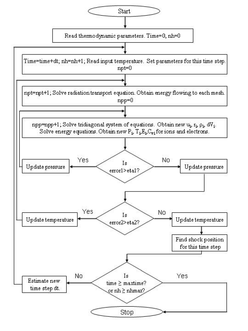
Figure 2: Flowchart for the Implicit 1D Radiation Hydrodynamics. Here, ’nh’ is the time step index and ’dt’ is the time step taken. The iteration indices for electron temperature and total pressure are expressed as ’npt’ and ’npp’ respectively. ’Error1’ and ’Error2’ are the fractional errors in pressure and temperature respectively whereas ’eta1’ and ’eta2’ are those acceptable by the error criterion.

The above procedure is repeated up to the time we are interested in following the evolution of the system. The solution method described above is clearly depicted in the flowchart given in Fig. 2. The time step index is denoted by ’nh’ and ’dt’ is the time step taken. The iteration indices for electron temperature and total pressure are expressed as ’npt’ and ’npp’ respectively. ’Error1’ and ’Error2’ are the fractional errors in pressure and temperature respectively whereas ’eta1’ and ’eta2’ are those acceptable by the error criterion.

2.4 Semi-implicit method

In the semi-implicit scheme, Eq. [5] is retained and $P_{i}^{1/2}$ is expressed as $P_{i}^{1/2}=(P_{i}+\tilde{P}_{i})/2$ wherein $\tilde{P}_{i}$ is the pressure at the end of the time step. Starting with the previous time step values for $\tilde{P}_{i}$, the position and velocity of each mesh is obtained and $\tilde{P}_{i}$ is iteratively converged using the EOS. As the variables are obtained explicitly from the known values, there is no need to solve the tridiagonal system of equations for the velocities of all the meshes [16]. Again, the energy flowing to the meshes as a result of radiation interaction is obtained by solving the transport equation once at the start of the time step, and hence the iterations leading to temperature convergence are absent.

3 Results

3.1 Investigation of the performance of the scheme using benchmark problems

3.1.1 Shock propagation in Aluminium

In the indirect drive inertial confinement fusion, high power laser beams are focused on the inner walls of high Z cavities or hohlraums, converting the driver energy to x-rays which implode the capsule. If the x-ray from the hohlraum is allowed to fall on an aluminium foil over a hole in the cavity, the low Z material absorbs the radiation and ablates generating a shock wave. Using strong shock wave theory, the radiation temperature in the cavity $T_{R}$ can be correlated to the shock velocity $u_{s}$. The scaling law derived for aluminium is $T_{R}=0.0126u_{s}^{0.63}$, where $T_{R}$ is in units of eV and $u_{s}$ is in units of cm/s for a temperature range of 100-250 eV [17].

For the purpose of simulation, an aluminium foil of thickness 0.6 mm and unit cross section is chosen. It is subdivided into 300 meshes each of width $2\times 10^{-4}$ cm. An initial guess value of $10^{-7}\mu s$ is used for the time step. The equilibrium density of Al is 2.71 gm/cc. In the discrete ordinates method four angles are chosen. As the temperature attained for this test problem is somewhat low, the total energy equation is solved assuming that electrons and ions are at the same temperature (the material temperature). The Equation of State (EOS) and Rosseland opacity for aluminium are given by

$$e=\frac{PV}{\gamma-1}=\epsilon T^{\mu}V^{\nu}$$ (50)

$$\kappa_{R}=l^{-1}T^{-\mu_{R}}V^{-\nu_{R}}$$ (51)

These power law functions, of temperature and density, where $\epsilon,l,\mu,\nu,\mu_{R}\ \mbox{and}\ \nu_{R}$ are the fitting parameters, are quite accurate in the temperature range of interest [18].

Using the fully implicit radiation hydrodynamics code, a number of simulations are carried out for different values of time independent incident radiation fluxes or temperatures. Corresponding shock velocities are then determined after the decay of initial transients. In Fig. 3. we show the comparison between the numerically obtained shock velocities for different radiation temperatures (dots) and the scaling law for aluminium (line) mentioned earlier. Good agreement is observed in the temperature range where the scaling law is valid .

Fig. 4. shows the various thermodynamic variables like velocity, pressure, density and material temperature after 2.5 ns when the radiation profile shown in Fig. 5. is incident on the outermost mesh . This radiation temperature profile (Fig. 5. ) is chosen so as to achieve a nearly isentropic compression of the fuel pellet. The pulse is shaped in such a way that the pressure on the target surface gradually increases, so that the generated shock rises in strength. From Fig. 4. we observe that the outer meshes have ablated outwards while a shock wave has propagated inwards. At 2.5 ns, the shock is observed at 0.5 mm showing a peak in pressure and density. As the outer region has ablated, they move outwards with high velocities. The outermost mesh has moved to 1.2 mm. The meshes at the shock front move inwards showing negative velocities. Also the temperature profile shows that the region behind the the shock gets heated to about 160 eV. In Fig. 6. we plot the distance traversed by the shock front as a function of time for the above radiation temperature profile. The shock velocity changes from 3.54 to 5.46 $cm/\mu s$ at 1.5 ns when the incident radiation temperature increases to 200 eV.

The performance of the implicit and semi-implicit schemes are compared by studying the convergence properties and the CPU cost for the problem of shock wave propagation in aluminium. The convergence properties are examined by obtaining the absolute $L_{2}$-Error in the respective thermodynamic variable profile versus the fixed time step value. The absolute $L_{2}$-Error in the variable $f$ (velocity, pressure, density or temperature) is defined as

$$L_{2}\mbox{-Error}=[\sum_{j=1}^{N}(f_{j}-f_{j}^{e})^{2}]^{1/2}$$ (52)

where the data $f_{j}^{e}$ constitute the exact solution for $\Delta t\longrightarrow 0$. This exact solution is chosen to be the result from a run using the implicit method with a small time step value of $10^{-10}\mu s$. The summation is taken over the values in all the meshes.

Fig. 7. shows the absolute $L_{2}$-Error versus the time step value for velocity, pressure, density and temperature obtained using the implicit and semi-implicit radiation hydrodynamics codes respectively. The semi-implicit differencing scheme fails for time steps of $10^{-5}\mu s$ and higher because of the violation of CFL criterion. For time steps $\sim 10^{-6}\mu s$, the errors obtained from the two schemes are comparable. But as the time steps are reduced, the implicit scheme converges very fast, i.e. the errors reduce quickly, whereas the error becomes nearly constant in the semi-implicit scheme because of the spatial discretization error. An initial mesh width of $2\times 10^{-4}$ cm is chosen for the above convergence study, which prevents further decrease in error in the semi-implicit scheme. Hence a reduction in the mesh width as well as the time steps is expected to decrease the error. In Fig. 8. the $L_{2}$-Error per mesh for velocity i.e. $[\sum_{j=1}^{N}(f_{j}-f_{j}^{e})^{2}/\mbox{number of meshes}]^{1/2}$, is plotted as a function of the time step by keeping the ratio of time step to mesh size i.e. $\Delta t/\Delta x$ constant at $5\times 10^{-3}\mu s/cm$. The results obtained from the implicit method using a small time step of $\Delta t=10^{-8}\mu s$ and mesh width of $2\times 10^{-6}$ cm is chosen as the exact solution. Both the implicit and semi-implicit schemes show linear convergence, though the convergence rate is faster for the implicit scheme showing its superiority in obtaining higher accuracies.

Fig. 9. shows that the faster convergence in the implicit method (Fig. 7.) is attained at the cost of slightly higher CPU time. However the cost in CPU seconds become comparable in the two schemes for smaller time steps. All the runs in this study were done on a Pentium(4) computer having 1GB of RAM operating at 3.4 GHz.

3.1.2 Point explosion problem

The self similar problem of a strong point explosion was formulated and solved by Sedov [19]. The problem considers a perfect gas with constant specific heats and density $\rho_{0}$ in which a large amount of energy $E$ is liberated at a point instantaneously. The shock wave propagates through the gas starting from the point where the energy is released. For numerical simulation, the energy E is assumed to be liberated in the first two meshes. The process is considered at a larger time $t$ when the radius of the shock front $R(t)>>r_{0}$, the radius of the region in which energy is released. It is also assumed that the process is sufficiently early so that the shock wave has not moved too far from the source. This ascertains that the shock strength is sufficiently large and it is possible to neglect the initial gas pressure $P_{0}$ or counter pressure in comparison with the pressure behind the shock wave [1].

Under the above assumptions the gas motion is determined by four independent variables, viz, amount of energy released $E$, initial uniform density $\rho_{0}$, distance from the centre of the explosion $r$ and the time $t$. The dimensionless quantity $\xi=r/R$ serves as the similarity variable. The motion of the wavefront $R(t)$ is governed by the relationship

$$R=\xi_{0}(\frac{E}{\rho_{0}})^{1/5}t^{2/5}$$ (53)

where $\xi_{0}$ is an independent variable. The propagation velocity of the shock wave is

$$D=\frac{2}{5}\xi_{0}^{5/2}(\frac{E}{\rho_{0}})^{1/2}R^{-3/2}$$ (54)

The parameters behind the shock front using the limiting formulas for a strong shock wave are

$$u_{1}=\frac{2}{\gamma+1}D$$ (55)

$$P_{1}=\frac{2}{\gamma+1}\rho_{0}D^{2}$$ (56)

$$\rho_{1}=\rho_{0}\frac{\gamma+1}{\gamma-1}$$ (57)

$$T_{1}=\frac{P_{1}}{(\gamma-1)\rho_{1}C_{V}}$$ (58)

where $C_{V}$ is the specific heat at constant volume and $\gamma=C_{P}/C_{V}$ is the ratio of the specific heats. The distributions of velocity, pressure and density w.r.t. the radius are determined as functions of the dimensionless variable $\xi=r/R$. Since the motion is self-similar, the solution can be expressed in the form

$$\ \ u=u_{1}(t)\tilde{u}(\xi),\ \ P=P_{1}(t)\tilde{P}(\xi),\ \ \rho=\rho_{1}\tilde{\rho}(\xi)$$ (59)

where $\tilde{u},\tilde{P}\ \mbox{and}\ \tilde{\rho}$ are new dimensionless functions. The hydrodynamic equations, which are a system of three PDE’s, are transformed into a system of three ordinary first-order differential equations for the three unknown functions $\tilde{u},\tilde{P}\ \mbox{and}\ \tilde{\rho}$ by substituting the expressions given by Eq. [59] into the hydrodynamic equations for the spherically symmetric case and transforming from r and t to $\xi$. The boundary condition satisfied by the solution at the shock front ($r=R\$ or $\xi=1$) is $\tilde{u}=\tilde{P}=\tilde{\rho}=1$. The dimensionless parameter $\xi_{0}$, which depends on the specific heat ratio $\gamma$ is obtained from the condition of conservation of energy evaluated with the solution obtained.

Also, the distributions of velocity, pressure, density and temperature behind the shock front are generated numerically using the hydrodynamics code without taking radiation interaction into account. Ideal D-T gas of density $\rho_{0}=1\ gm/cc$ and $\gamma=1.4$ is filled inside a sphere of 1 cm radius with the region divided into 100 radial meshes each of width $0.01\ cm$. The initial internal energy per unit mass is chosen as $10^{5}\ Tergs/gm$ for the first two meshes and zero for all the other meshes. An initial time step of $10^{-}6\ \mu s$ is chosen and the thermodynamic variables are obtained after a time $0.2\ \mu s$. As in the case of the problem of shock propagation in aluminium, the total energy equation is solved assuming that electrons and ions are at the same temperature (the material temperature). In Fig. 10. we compare the distribution of the functions $P/P_{1},u/u_{1},\rho/\rho_{1}\ \mbox{and}\ T/T_{1}$ with respect to $r/R$ obtained exactly by solving the ODEs as explained above (solid lines) with the results generated from our code (dots). Good agreement between the numerical and theoretical results is observed. As is characteristic of a strong explosion, the gas density decreases extremely rapidly as we move away from the shock front towards the centre as seen from Fig. 10. In the vicinity of the front the pressure decreases as we move towards the centre by a factor of 2 to 3 and then remains constant whereas the velocity curve rapidly becomes a straight line passing through the origin.The temperatures are very high at the centre and decreases smoothly at the shock front. As the particles at the centre are heated by a strong shock, they have very high entropy and hence high temperatures.

The radiation interaction effects become prominent only at higher temperatures. The Rosseland opacity of a D-T (50:50) gas in terms of the gas density and temperature is $\kappa_{R}=0.505\ \rho^{2}\ T^{7/2}$ [20], [1]. Fig. 11. shows the profiles of velocity, pressure, density and temperature after $2\ \mu s$ with an initial specific internal energy of $10^{5}\ Tergs/gm$ deposited in the first two meshes (i.e. total energy deposited is 3.351 Tergs = $3.351\times 10^{12}\mbox{ergs}$ ), $\gamma=1.23$ and 200 meshes each of width $0.01\ cm$. The shock front moves faster in the pure hydrodynamic case as no energy is lost to the radiation keeping the shock stronger. Also the effect of radiation interaction is to reduce the temperature at the centre as seen in Fig. 11(d).

The convergence study for the point explosion problem shows that the $L_{2}$-Error decreases much faster for the implicit method compared to the explicit scheme as observed in Fig. 12. The exact solution in this case is chosen to be the result from a run using the implicit method with a small time step value of $10^{-8}\mu s$ and an initial mesh width of $0.01\ cm$. As the time step is decreased, the non-linearities are iteratively converged for the implicit scheme, whereas for the explicit scheme, the spatial discretization error begins to dominate thereby preventing any appreciable decrease in the $L_{2}$-Error (as observed in the problem of shock propagation in aluminium foil also). In the implicit method, faster convergence is attained at the cost of slightly higher CPU time as shown in Fig. 13.

4 Conclusions

In this paper we have developed and studied the performance of fully implicit radiation hydrodynamics scheme as compared to the semi-implicit scheme. The time dependent radiation transport equation is solved and energy transfer to the medium is accounted exactly without invoking approximation methods. To validate the code, the results have been verified using the problem of shock propagation in Al foil in the planar geometry and the point explosion problem in the spherical geometry. The simulation results show good agreement with the theoretical solutions. The convergence properties show that the $L_{2}$-Error keeps on decreasing on reducing the time step value for the implicit scheme. However for the semi-implicit scheme, the $L_{2}$-Error remains fixed below a certain time step because of the spatial discretization error showing that the implicit scheme is necessary if high accuracy is to be obtained. Also the price to be paid for obtaining such high accuracies is only slightly higher than the semi-implicit scheme in terms of the CPU time. The implicit scheme gives fairly accurate result even for large time steps whereas the semi-implicit scheme does not work there because of the CFL criterion.

Figure 1: Grid structure.

Figure 3: Comparison of simulation data (dots) with scaling law (line) relating shock velocity with the radiation temperature for aluminium.

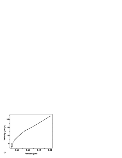
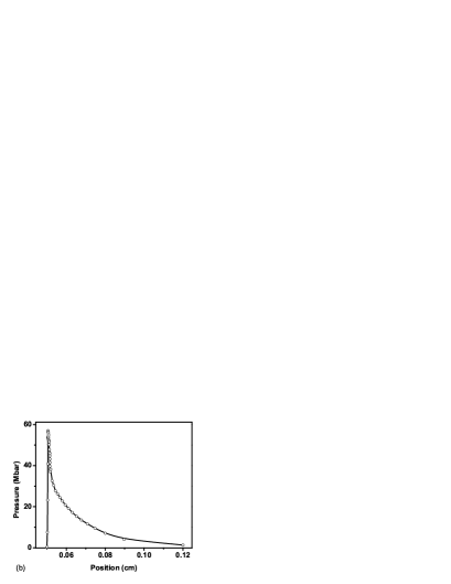
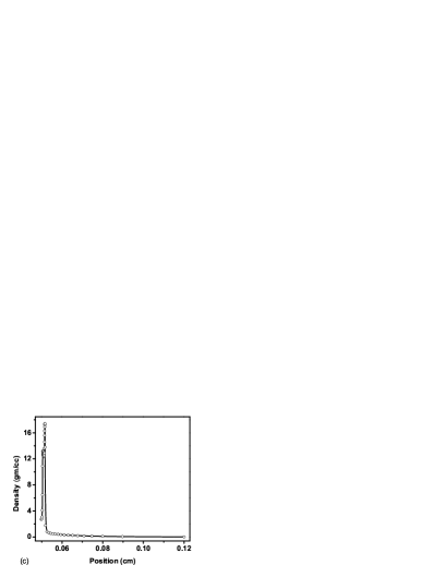
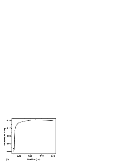
Figure 4: Profiles of the thermodynamic variables like (a) velocity, (b) pressure, (c) density and (d) temperature in the region behind the shock as a function of the distance at t = 2.5 ns. The region ahead of the shock is undisturbed and retain the initial values of the variables. The incident radiation temperature on the Al foil is shown in Figure 5.

Figure 5: Radiation temperature profile in the hohlraum for strong shock propagation in aluminium.

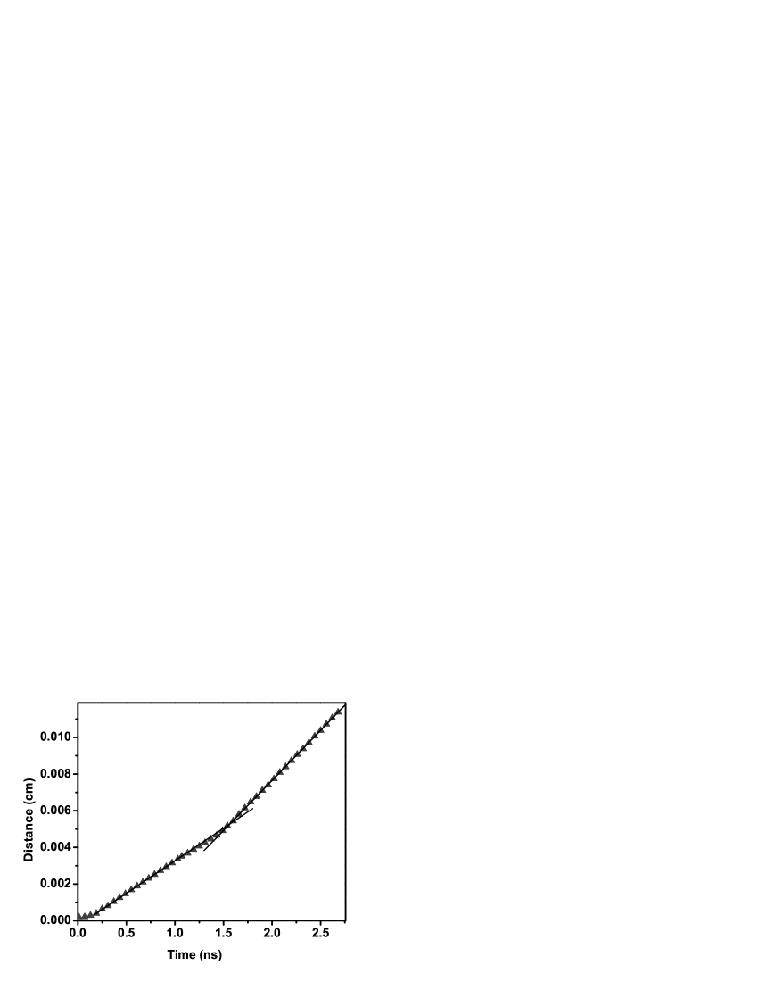
Figure 6: Distance traversed by the shock front vs. time graph in Al foil for the incident radiation temperature shown in Figure 5. The two slopes correspond to the two plateaus in the radiation profile.

Figure 7: Comparison of the $L_{2}$-Error Vs. time step for the shock wave propagation problem in aluminium with mesh width $\Delta x=2\times 10^{-4}$ cm. Convergence is faster in the implicit scheme.

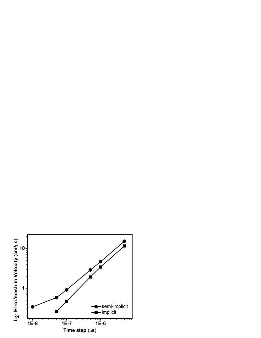
Figure 8: $L_{2}$-Error/mesh in velocity Vs. time step for the shock wave propagation problem in aluminium with $\Delta t/\Delta x=5\times 10^{-3}\mu s/cm$. Convergence rate is higher for the implicit scheme.

Figure 9: CPU cost Vs. time step for the shock wave propagation problem in aluminium with mesh width $\Delta x=2\times 10^{-4}$ cm.

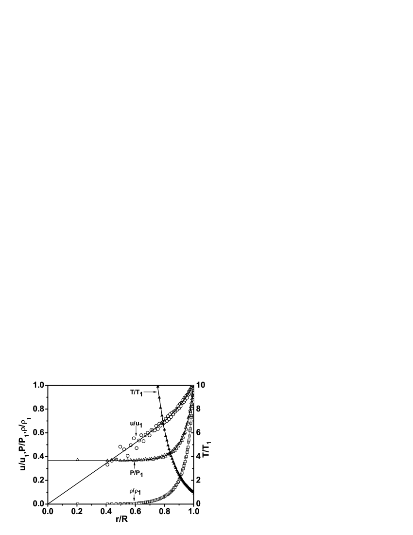
Figure 10: Comparison of the simulation data obtained in the pure hydrodynamic case (points) with the self similar solutions (lines) for the point explosion problem with specific internal energy $E=10^{5}\$Tergs/gm deposited in the first two meshes and $\gamma=1.4$ .

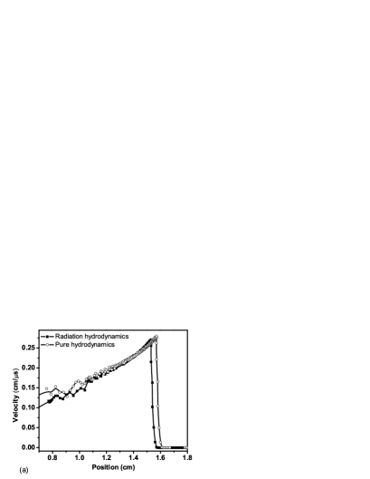
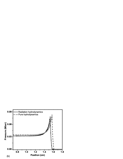
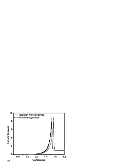
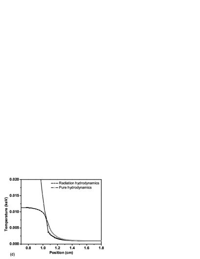
Figure 11: Profiles of the thermodynamic variables with and without radiation interaction at $2\ \mu s$ for the point explosion problem with specific internal energy $E=10^{5}\$Tergs/gm deposited in the first two meshes.

Figure 12: Comparison of the $L_{2}$-Error Vs. time step for the point explosion problem. Implicit scheme converges faster.

Figure 13: CPU cost for the point explosion problem with specific internal energy $E=10^{5}\$Tergs/gm deposited in the first two meshes for the implicit and semi-implicit schemes taking radiation interaction into account.

References

- [1] Y.B.Zeldovich and Y.P.Raizer, Physics of Shock Waves and High-Temperature Hydrodynamic Phenomena, Vols I and II (Academic Press, New York, 1966)
- [2] D.Mihalas and B.W.Mihalas, Foundations of Radiation Hydrodynamics (Oxford Univ.Press, New York, 1984)
- [3] J.W.Bates, et.al., On Consistent Time-Integration Methods for Radiation Hydrodynamics in the Equilibrium Diffusion Limit: Low-Energy-Density Regime, J.Comput.Phys. 167, 99 (2001)
- [4] W.dai and P.R.Woodward, Numerical simulation for radiation hydrodynamics I. Diffusion limit, J.Comput.Phys. 142, 182 (1998)
- [5] W.dai and P.R.Woodward, Numerical simulation for radiation hydrodynamics II. Transport limit, J.Comput.Phys. 157, 199 (2000)
- [6] D.A.Knoll, W.J.Rider, G.L.Olson, Nonlinear convergence, accuracy, and time step control in nonequilibrium radiation diffusion, Journal of Quantitative Spectroscopy and Radiative Transfer 70, 25 (2001)
- [7] C.C.Ober and J.N.Shadid, Studies on the accuracy of time-integration methods for the radiation-diffusion equations, J.Comput.Phys. 195, 743 (2004)
- [8] D.A.Knoll, L.Chacon, L.G.Margolin, V.A.Moussean, On balanced approximations for time integration of multiple time scale systems, J.Comput.Phys. 185, 583 (2003)
- [9] D.de Neim, E.Kuhrt, U.Motschmann, A volume-of-fluid method for simulation of compressible axisymmetric multi-material flow, Comput. Phys. Commun. 176, 170 (2007)
- [10] J. Von Neumann and R.D.Richtmyer, A Method for the Numerical Calculation of Hydrodynamic Shocks, J. Appl. Phys. 21, 232 (1950)
- [11] Huba J D. 2006 NRL Plasma Formulary (Washington: Naval Research Lab.) 35
- [12] E.Larsen, A Grey Transport Acceleration Method for Time-Dependent Radiative Transfer Problems, J.Comput.Phys. 78, 459 (1988)
- [13] E.E.Lewis and W.F.Miller, Jr., Computational Methods of Neutron Transport, (John Wiley and Sons, New York, 1984)
- [14] P.Barbucci and F.Di Pasquantonio, Exponential Supplementary Equations for Methods: The One-Dimensional Case, Nucl. Sci. Eng. 63, 179 (1977)
- [15] M.L.Wilkins, Computer Simulation of Dynamic Phenomena (Springer-Verlag, Berlin, Heidelberg, New York, 1999) ISBN 3-540-63070-8
- [16] R.D.Richtmyer and K.W.Morton, Difference Methods for Initial-Value Problems, Second Edition (Interscience Publishers, New York, 1967)
- [17] R.L.Kauffman, et.al, High Temperatures in Inertial Confinement Fusion Radiation Cavities heated with light, Phys. Rev. Lett. 73, 2320 (1994)
- [18] M.Basko, An improved version of the view factor method for simulating inertial confinement fusion hohlraums, Phys. Plasmas 3, 4148 (1996)
- [19] L.I.Sedov, Similarity and Dimensional Methods in Mechanics (Gostekhizdat, Moscow, 4 th edition 1957. English transl. (M.Holt, ed.), Academic Press, New York, 1959)
- [20] S.L.Thompson and H.S.Lauson, Improvements in the Chart D Radiation-Hydrodynamic Code III: Revised Analytic Equation of State, Sandia Laboratories, SC-RR-71 0714 (1972)