Broad reprocessed Balmer emission from warped accretion discs

Abstract

Double peaked broad emission lines in active galactic nuclei are generally considered to be formed in an accretion disc. In this paper, we compute the profiles of reprocessing emission lines from a relativistic, warped accretion disc around a black hole in order to explore the possibility that certain asymmetries in the double-peaked emission line profile which can not be explained by a circular Keplerian disc may be induced by disc warping. The disc warping also provides a solution for the energy budget in the emission line region because it increases the solid angle of the outer disc portion subtended to the inner portion of the disc. We adopted a parametrized disc geometry and a central point-like source of ionizing radiation to capture the main characteristics of the emission line profile from such discs. We find that the ratio between the blue and red peaks of the line profiles becoming less than unity can be naturally predicted by a twisted warped disc, and a third peak can be produced in some cases. We show that disc warping can reproduce the main features of multi-peaked line profiles of four active galactic nuclei from the Sloan Digital Sky Survey.

Accepted . Received ; in original form

1 Introduction

A small fraction of active galactic nuclei (AGN) show double-peaked broad emission line profiles (Eracleous & Halpern, 1994, 2003; Strateva et al., 2003; Gezari, Halpern & Eracleous, 2007). The possibility has been considered for a long time that at least some of these lines arise directly from the accretion discs assumed to feed the central supermassive black holes. The H$\alpha$ profile observed in the spectrum of Arp 102B was modelled as arising in a relativistic disc by Chen & Halpern (1989) and Chen, Halpern & Filippenko (1989) in an attempt to explain the asymmetric double-peaked profiles. In these stationary circular relativistic disc models, Doppler boosting will make the blue peak of the profile higher than the red one. However, Miller & Peterson (1990) questioned the relativistic disc explanation for Arp 102B, by showing that at least at some epochs the profile asymmetry is reversed, with the red peak higher than the blue one in contrary to the prediction of homogeneous, circular relativistic disc models. This type of profile asymmetry has been observed in some other double-peaked sources (Strateva et al., 2003; Gezari et al., 2007). Thus, other scenarios for the profile asymmetry were considered later on, including various physically plausible processes in the accretion flow, such as spiral shocks, eccentric discs, bipolar outflows (Chakrabarti & Wiita, 1993, 1994; Eracleous et al., 1995; Storchi-Bergmann et al., 1997; Zheng, Sulentic & Binette, 1990; Veilleux & Zheng, 1991), as well as a binary black hole system (Begelman, Blandford & Rees, 1980; Gaskell, 1996; Zhang, Dultzin-Hacyan & Wang, 2007b).

In addition to the line profile asymmetry, the energetic budget for the line emission region has not been solved so far for the disc model. It is demonstrated that the local viscous heating in the accretion disc is not sufficient to explain the observed H$\alpha$ intensity (Chen et al., 1989; Eracleous et al., 1997), thus reprocessing of ultraviolet(UV)/X-ray continuum from the inner accretion disc is required. However, only a very small fraction of radiation from inner disc is expected to intercept the outer part of the disc in the case of a flat geometrically thin disc. Two type of processes have been proposed to increase the fraction of light incident on to the disc emission-line region. Chen et al. (1989) proposed that the inner part of the accretion disc is hot and becomes geometrically thick due to insufficient radiative cooling, and the X-ray emission from such an ion-supported torus is responsible for such energy input. However, double peak emitters do not always have a low accretion rate (Zhang, Dultzin-Hacyan & Wang, 2007a; Bian et al., 2007). Furthermore, a detailed calculation of advection dominated accretion flow (ADAF) models suggests that only a small portion of X-rays actually hit the emission-line portion of the disc (Cao & Wang, 2006). On the other hand, Cao & Wang (2006) proposed that a slow moving jet can scatter a substantial fraction of UV/X-ray light from the inner accretion disc back to the outer part of the disc. While this may be the likely case for radio-loud double-peaked emitters, the majority of double-peaked emitters are radio quiet.

On the other hand, warped accretion discs are believed to exist in a variety of astrophysical systems, including X-ray binaries, T Tauri stars, and AGN. The dynamics of warping accretion discs has been discussed by a number of authors (Papaloizou & Pringle, 1983; Papaloizou & Lin, 1995; Ogilvie, 1999; Nelson & Papaloizou, 1999, 2000; Nayakshin, 2005). Four main mechanisms for exciting/maintaining warping in accretion discs have been proposed, including: tidally induced warping by a companion in a binary system (Terquem & Bertout, 1993, 1996; Larwood et al., 1996), radiation driven or self-inducing warping (Pringle, 1996, 1997; Maloney, Begelman & Pringle, 1996; Maloney & Begelman, 1997; Maloney, Begelman & Nowak, 1998), magnetically driven disc warping (Lai, 1999, 2003; Pfeiffer & Lai, 2004), and frame dragging driven warping (Bardeen & Petterson, 1975; Kumar & Pringle, 1985; Armitage & Natarajan, 1999). As a result, the accretion disc in some AGN should be nonplanar. Evidence for the existence of warped discs in AGN has been found by observations (Herrnstein et al., 2005; Caproni et al., 2007). A warped disc makes it possible for the radiation from the inner disc to reach the outer parts, enhancing the reprocessing emission lines. Thus, this warping can solve the long-standing energy-budget problem because the subtending angle of the outer disc portion to the inner part has been increased by the warp. It can also provide the asymmetry required for the variations of the emission lines. The effect of disc warping on iron line profiles treated relativistically have been made by Hartnoll & Blackman (2000) and Čadež et al. (2003). Bachev (1999) studied the broad-line H$\beta$ profiles from a warped disc. Nevertheless, his treatment is non-relativistic. A relativistic treatment of warped disc on the Balmer lines which can be compared with observations is still not available in the literature.

In this paper, the broad Balmer emission due to reprocessing of the central high-energy radiation by a warped accretion disc is investigated. Our main purpose here is to describe the effect of disc warping on the line profiles. A parametrized disc model is adopted. In §2 we summarize the assumptions behind our model, and present the basic equations relevant to our problem. We present our results and the comparison with observations in §3, and conclusion and discussion in §4.

2 Assumptions and Method of Calculation

In this paper, we will focus on how a warped disc affects the optical emission-line profiles, such as H$\alpha$ and H$\beta$. A geometrically thin disc and a central point-like source of ionizing radiation around a black hole are assumed.

2.1 Geometrical considerations

The disc can be treated as being composed of a series of concentric circular rings of increasing radii, and laying in different planes. The rings interact with each other via viscous stresses. Each ring is defined by two Eulerian angles $\beta(R,t)$ and $\gamma(R,t)$ (see Fig.1) at radius $R$, where $\beta(R,t)$ is the tilt angle of the disc with respect to the normal to the equatorial plane, while the twist angle $\gamma(R,t)$ describes the orientation of the line of nodes with respect to a fixed axis in the equatorial plane. Note that $R$ is a purely radial coordinate and not the cylindrical one. At each radius $R$ from the center, the disc has a unit tilt vector $\mbox{\boldmath$l$}(R,t)$ which varies continuously with radius $R$ and time $t$. Following Pringle (1996), in an inertial frame $\rm OXYZ$ centered on the disc, the vector $\mbox{\boldmath$l$}(R,t)$ is given by

$$\mbox{\boldmath$l$}=(\cos\gamma\sin\beta,\sin\gamma\sin\beta,\cos\beta).$$ (1)

We define the normalized vector towards the observer as

$$\mbox{\boldmath$i$}_{obs}=(\sin i,0,\cos i),$$ (2)

where $i$ is the angle between the line of sight and the normal to the equatorial plane lie in the $\rm XZ$ plane.

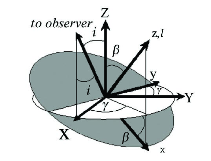
Figure 1: The geometry used in this paper. The warped accretion disc is modeled as a collection of inclined rings, each defined by two Eulerian angles $\beta,\gamma$ and the radial distance $R$. The normal to the equatorial plane is aligned with the $\rm Z$ direction. The direction to the observer is denoted by $i$ that is the angle between the direction of line of sight and the $\rm Z$-axis.

We define the coordinates on the surface of the disc as ($R,\phi$) with respect to a fixed Cartesian coordinate system $(x,y,z)$, where $\phi$ is the azimuthal angle measured on the disc surface in the direction of flow, with $\phi=\pi/2$ at the ascending node. The position vector of a point on the ring of radius $R$ is $\mbox{\boldmath$R$}=R\,\mbox{\boldmath$e$}_{R}$, where

$$\mbox{\boldmath$e$}_{R}=\left[\matrix{\cos\gamma\cos\beta\cos\phi-\sin\gamma\sin\phi\cr\sin\gamma\cos\beta\cos\phi+\cos\gamma\sin\phi\cr-\sin\beta\cos\phi}\right]$$ (3)

is the radial unit vector. Note that $\mbox{\boldmath$l$}\cdot\mbox{\boldmath$e$}_{R}=0$, since points on the ring lie in the plane that passes through the origin and is orthogonal to $l$. Now $(R,\phi)$ are (in general) non-orthogonal coordinates on the surface of the disc. The element of surface area is

$${\rm d}\mbox{\boldmath$S$}=\left({{\partial\mbox{\boldmath$R$}}\over{\partial R}}\,{\rm d}R\right)\times\left({{\partial\mbox{\boldmath$R$}}\over{\partial\phi}}\,{\rm d}\phi\right),$$ (4)

by calculating these partial derivatives directly and after some algebra which simplifies to

$${\rm d}\mbox{\boldmath$S$}=\left[\mbox{\boldmath$l$}+(R\beta^{\prime}\cos\phi+R\gamma^{\prime}\sin\beta\sin\phi)\,\mbox{\boldmath$e$}_{R}\right]R\,{\rm d}R\,{\rm d}\phi,$$ (5)

where the primes indicate differentiation with respect to $R$, and hence, since $\mbox{\boldmath$l$}\cdot\mbox{\boldmath$e$}_{R}=0$, that

$$|{\rm d}\mbox{\boldmath$S$}|=\left[1+(R\beta^{\prime}\cos\phi+R\gamma^{\prime}\sin\beta\sin\phi)^{2}\right]^{1/2}R\,{\rm d}R\,{\rm d}\phi.$$ (6)

The radiation flux ${\rm L}$ received from the central parts by the unit area is proportional to

$${\rm L}\propto\frac{\displaystyle|(R\beta^{\prime}\cos\phi+R\gamma^{\prime}\sin\beta\sin\phi)|}{\displaystyle R^{2}\left[1+(R\beta^{\prime}\cos\phi+R\gamma^{\prime}\sin\beta\sin\phi)^{2}\right]^{1/2}},$$ (7)

if the element in question is not obscured by other interior parts of the disc, otherwise the flux is set to zero (see below). The Balmer lines in the illuminated surface is formed as a result of photoionization by UV/X-ray radiation from inner accretion disc. We assume that Balmer line intensity is proportional to the radiation being intercepted by the disc, thus the line emissivity $\varepsilon$ on the disc surface can take the form: $\varepsilon\propto{\rm L}$. A detailed treatment of line emission requires solving the vertical structure as well as the radiative transfer in the disc explicitly, which is beyond the scope of this paper. We also assume that the line emission is isotropic in the comoving frame.

An alternative useful formalism being used to describe the shape of the warped disc is introducing the scale-height of the disc which is the displacement in the direction normal to the equatorial plane. The scale-height denoted by $h(r,\varphi)$ is a function of radius $r$ and azimuthal angle $\varphi$ in cylindrical coordinates with respect to Cartesian coordinate system ${\rm(X,Y,Z)}$. The two formalisms described above can be related by the formula

$$h(r,\varphi) = -R\sin\beta\cos\phi$$ (8)

$$= -R\sin\beta\cos\psi\big{/}\sqrt{1-\sin^{2}\beta\sin^{2}\psi}$$

$$= -r\tan\beta\cos\psi.$$

Where $\psi=\varphi-\gamma$ and satisfies

$$\tan\phi\,=\,\tan\psi\cos\beta.$$ (9)

Since it is difficult to calculate analytically the disc distortion induced by combined action of external torques mentioned above, here we do not consider the disc dynamics, and merely parametrize the disc geometry to capture the main characteristics of emission-line profiles from warped discs. In this paper, a steady disc is adopted, and the form of the two angles $\gamma$, $\beta$ as a function of radial $R$ are given by

$$\gamma = \gamma_{0}+n_{1}e^{n_{2}\frac{R_{in}-R}{R_{out}-R_{in}}},$$ (10)

$$\beta = n_{3}\sin\left[\frac{\pi}{2}\left(\frac{R-R_{in}}{R_{out}-R_{in}}\right)\right].$$ (11)

Where $R_{in}$ and $R_{out}$ are the disc inner and outer radii, $n_{i}~{}(i=1,2,3)$ are three free parameters used to describe the warped disc geometry, $\gamma_{0}$ is a constant which is used to describe the longitude of the observer with respect to the coordinate system of the disc. This angle is mathematically equivalent to changing observational time for possible precession. Thus, the line profiles with different $\gamma_{0}$ can be compared with the data observed at different times.

2.2 Photon motions in the background metric

The propagation of radiation from the disc around a Kerr black hole and the particle kinematics in the disc were studied by many authors (Carter, 1968; Bardeen, Press & Teukolsky, 1972). We review properties of the Kerr metric and formulae for its particle orbits, and summarize here the basic equations relevant to this paper. Throughout the paper we use units in which $G=c=1$, where $G$ is the gravitational constant, $c$ is the speed of light. In Boyer-Lindquist coordinates, the Kerr metric is given by

$$ds^{2} = -e^{2\nu}dt^{2}+e^{2\psi}(d\phi-\omega dt)^{2}+\frac{\Sigma}{\Delta}dr^{2}+\Sigma d\theta^{2},$$ (12)

where

$$e^{2\nu}=\Sigma\Delta/A,\,e^{2\psi}=\sin^{2}\theta A/\Sigma,\,\omega=2Mar/A,$$

$$\Sigma=r^{2}+a^{2}\cos^{2}\theta,\,\Delta=r^{2}+a^{2}-2Mr,$$

$$A=(r^{2}+a^{2})^{2}-a^{2}\Delta\sin^{2}\theta.$$

Here $M$, $a$ are the black hole mass and specific angular momentum, respectively.

The general orbits of photons in the Kerr geometry can be expressed by a set of three constants of motion (Carter, 1968). Those are the energy at infinity $E$, the axial component of angular momentum $E\lambda$, and carter’s constant ${\cal Q}\,({=}q^{2}E^{2})$. The 4-momentum of a geodesic has components

$$p_{\mu}=(p_{\rm t},\,p_{\rm r},\,p_{\theta},\,p_{\phi})=(-E,\,\pm E\sqrt{R}/\Delta,\,\pm E\sqrt{\Theta},\,E\lambda),$$ (13)

with

$$R = r^{4}+\left(a^{2}-\lambda^{2}-q^{2}\right)r^{2}+2M\left[q^{2}+(\lambda-a)^{2}\right]r-a^{2}q^{2}\;,$$

$$\Theta = q^{2}+a^{2}\cos^{2}\theta-\lambda^{2}\cot^{2}\theta\;.$$

From this, the equations of motion governing the orbital trajectory can be obtained. The motion in the $r$-$\theta$ plane is governed by (Bardeen et al., 1972)

$$\int_{r_{e}}^{r}\frac{dr}{\sqrt{R(r)}}=\pm\int_{\theta_{e}}^{\theta}\frac{d\theta}{\sqrt{\Theta(\theta)}}\;,$$ (14)

where $r_{e}$ and $\theta_{e}$ are the starting values of $r$ and $\theta$. The $\phi$ coordinate along the trajectory is calculated by (Wilkins, 1972; Viergutz, 1993)

$$\int_{\phi_{e}}^{\phi}{\rm d}\phi=\int_{\theta_{e}}^{\theta}\frac{\lambda{\rm d}\theta}{\sin^{2}\theta\sqrt{\Theta(\theta)}}+\int_{r_{e}}^{r}\frac{(2ar-\lambda a^{2}){\rm d}r}{\Delta\sqrt{R(r)}}.$$ (15)

Consider the orbit equation in the form

$$\int_{r_{ms}}^{r}\frac{dr}{\sqrt{R(r)}}=\pm\int_{\pi/2}^{\theta}\frac{d\theta}{\sqrt{\Theta(\theta)}}=P\;,$$ (16)

where $r_{ms}$ is the radius of the marginally stable orbit for a maximal Kerr black hole, $a=0.998$. Then $\theta$ can be expressed in terms of $P$ as follows (Čadež, Fanton & Calvani, 1998)

$$\cos\theta(r)=\mu_{+}{\rm cn}(a\sqrt{\mu_{+}^{2}+\mu_{-}^{2}}P\pm K(m)|m)\;,$$ (17)

where $m=\frac{\mu_{+}^{2}}{\mu_{+}^{2}+\mu_{-}^{2}}$, $\mu_{\pm}^{2}$ are defined by

$$\mu_{\pm}^{2}=\frac{1}{2a^{2}}\left\{\left[\left(\lambda^{2}+q^{2}-a^{2}\right)^{2}+4a^{2}q^{2}\right]^{1/2}\mp\left(\lambda^{2}+q^{2}-a^{2}\right)\right\}\;.$$ (18)

and

$$K(m)={\rm cn}^{-1}\left(\left.0\right|m\right).$$ (19)

Where $K(m)$ is the complete elliptic integral of the first kind.

For photons emitted from radii ($>$100$r_{g}$) propagating to infinity the differences between Kerr and Schwarzschild black holes are indistinguishable. Neglecting terms of order $1/r^{2}$ and higher, the Kerr metric reduces to the Schwarzschild metric. The formulae for the particle orbits in this case are simplified. Here we summarize the basic equations relevant to this paper. The line element in Schwarzschild geometry is written as follows:

$${\rm d}s^{2}=-(1-2/r){\rm d}t^{2}+\frac{1}{1-2/r}{\rm d}r^{2}+r^{2}{\rm d\vartheta}^{2}+r^{2}{\rm sin}^{2}\vartheta{\rm d}\phi^{2}.$$ (20)

The observer is assumed to be located at ($r_{\rm o},\vartheta_{\rm o},\phi_{\rm o}$). For a approximately spherical background, each inclined ring of the disc can be considered lying in the equatorial plane. Owing to a spherically symmetric metric there is no favored direction for the black hole; in this sense, $\vartheta_{\rm o}$ can be acted as the angle between the observer and the normal to the disc and is determined by taking the dot-products of the unit vector $l$ of the disc with the normalized vector $\mbox{\boldmath$i$}_{\rm obs}$ to the observer. By definition, we get

$$\cos\vartheta_{\rm o}=\cos\gamma\sin\beta\sin i+\cos\beta\cos i$$ (21)

The angle $\phi_{\rm 0}$ can be obtained by setting the mixed triple product of three vectors $\mbox{\boldmath$i$}_{\rm obs},\mbox{\boldmath$l$}$ and $\mbox{\boldmath$e$}_{\rm R}$ equal zero, $(\mbox{\boldmath$i$}_{\rm obs}\;\mbox{\boldmath$l$}\;\mbox{\boldmath$e$}_{\rm R})=0$. From this equation, the angle is determined by

$$\tan\phi_{\rm o}=\frac{\sin\gamma\sin i}{\sin\beta\cos i-\cos\beta\cos\gamma\sin i}.$$ (22)

The photon motion equations are given by (Lu & Yu, 2001):

$$\int_{r_{e}}^{r}\frac{dr}{\sqrt{R(r)}}=\pm\int_{\vartheta_{e}}^{\vartheta}\frac{d\vartheta}{\sqrt{\Theta(\vartheta)}}\;,$$ (23)

$$\int_{\phi_{e}}^{\phi}{\rm d}\phi=\pm\int_{\vartheta_{e}}^{\vartheta}\frac{\lambda{\rm d}\vartheta}{{\rm sin}^{2}\vartheta\sqrt{\Theta(\vartheta)}}.$$ (24)

where $r_{e}$, $\vartheta_{e}$ and $\phi_{e}$ are the starting values of $r$, $\vartheta$ and $\phi$.

Define $\mu=\cos\vartheta$, then in equations (23) and (24) the integral over $\mu$ can be worked out in terms of a trigonometric integral

$$\int_{\pi/2}^{\vartheta}\frac{d\vartheta}{\sqrt{\Theta(\vartheta)}} = \int_{0}^{\mu}\frac{d\mu}{\sqrt{q^{2}-\left(\lambda^{2}+q^{2}\right)\mu^{2}}}$$ (25)

$$= \frac{1}{\sqrt{\lambda^{2}+q^{2}}}\,\rm{sin^{-1}\left(\mu/\mu_{+}\right)},$$

$$\int_{\pi/2}^{\vartheta}\frac{\lambda{\rm d}\vartheta}{{\rm sin}^{2}\vartheta\sqrt{\Theta(\vartheta)}} = \int_{0}^{\mu}\frac{\lambda d\mu}{(1-\mu^{2})\sqrt{\Theta_{\mu}(\mu)}}$$ (26)

$$= \pm\rm{sin^{-1}\sqrt{\frac{(1-\mu_{+}^{2})\mu^{2}}{\mu_{+}^{2}(1-\mu^{2})}}}.$$

Where $0\leq\mu<\mu_{+}$ ,  $\mu_{+}=\sqrt{q^{2}/(\lambda^{2}+q^{2})}$ and $\Theta_{\mu}(\mu)=q^{2}-(\lambda^{2}+q^{2})\mu^{2}$. The integral over $r$ can be worked out with inverse Jacobian elliptic integrals (see e.g. Čadež et al., 1998; Wu & Wang, 2007).

Although our calculation is limited to Schwarzschild metric for photons travelling to infinity, for the radii ($>$100 $r_{\rm g}$) taken into account in this paper, the results are essentially the same for the Kerr black hole. On the other hand, for the light from inner part of the disc, a maximal Kerr metric is still used.

2.3 The observed line flux

Due to relativistic effects, the photon frequency will shift from the emitted frequency $\nu_{\rm e}$ to the observed one $\nu_{\rm o}$ received by a rest observer with the hole at infinity. We introduce a $g$ factor to describe the shift which is the ratio of observed frequency to emitted one:

$$g = \nu_{\rm o}/\nu_{\rm e}=(\mbox{\boldmath$p$}\cdot\mbox{\boldmath$u$}_{\rm o})/(\mbox{\boldmath$p$}\cdot\mbox{\boldmath$u$}_{\rm e})$$ (27)

$$= (1-\Omega\lambda)^{-1}\sqrt{1-\frac{3}{r}},$$

where $\Omega=r^{-3/2}$ is the Keplerian angular velocity, $\mbox{\boldmath$p$},\mbox{\boldmath$u$}_{\rm o},\mbox{\boldmath$u$}_{\rm e}$ are the 4-momentum of the photon, the 4-velocity of the observer and the emitter, respectively.

The specific flux density $F_{\rm o}(\nu_{\rm o})$ at frequency $\nu_{\rm o}$ as observed by an observer at infinity is defined as the sum of the observed specific intensities $I_{\rm o}(\nu_{\rm o})$ from all parts of the accretion disc surface, which is given by (Cunningham, 1975)

$$F_{\rm o}(\nu_{\rm o}) = \int I_{\rm o}(\nu_{\rm o})d\Omega_{\rm obs}$$ (28)

$$= \int g^{3}I_{\rm e}(\nu_{\rm e})d\Omega_{\rm obs}\;.$$

where $d\Omega_{\rm obs}$ is the element of the solid angle subtended by the image of the disc on the observer’s sky and we have made use of the relativistic invariance of $I_{\nu}/\nu^{3}$, $\nu$ is the photon frequency measured by any local observer on the path.

$I_{\rm e}(\nu_{\rm e})$ is the specific intensity measured by an observer corotating with the disc, and can be approximated by a $\delta$-function, $I_{\rm e}^{\prime}(\nu_{\rm e}^{\prime})=\varepsilon\delta(\nu_{\rm e}^{\prime}-\nu_{\rm e})$, where $\varepsilon$ is the emissivity per unit surface area. From well-known transformation properties of $\delta$-functions we have $\delta(\nu_{\rm e}^{\prime}-\nu_{\rm e})=g\delta(\nu_{\rm o}-g\nu_{\rm e})$, using this in equation (28), we obtain

$$F_{\rm o}(\nu_{\rm o})=\int\varepsilon g^{4}\delta(\nu_{\rm o}-g\nu_{\rm e})d\Omega_{\rm obs}\;.$$ (29)

In order to calculate the integration over $d\Omega_{\rm obs}$, using two impact parameters $\alpha$ and $\beta$, measured relative to the direction to the centre of the black hole, firstly introduced by Cunningham & Bardeen (1973) is convenient. They are related to two constants of motion $\lambda$ and $q$ by equations

$$\alpha=-\lambda/\sin\vartheta_{\rm o},\,\beta=\pm\left(q^{2}-\lambda^{2}\cot^{2}\vartheta_{\rm o}\right)^{1/2}\!,$$ (30)

The element of solid angle seen by the observer is then

$$d\Omega_{\rm obs}=\frac{d\alpha d\beta}{r_{\rm o}^{2}}=\frac{q}{r_{\rm o}^{2}\beta\sin\vartheta_{\rm o}}\frac{\partial(\lambda,q)}{\partial(r,g)}\;dr\;dg,$$ (31)

where $r_{\rm o}$ is the distance from the observer to the black hole.

Substituting equation (31) into equation (29) gives the desired result:

$$F_{\rm o}(\nu_{\rm o}) = \frac{q}{r_{\rm o}^{2}\beta\sin\vartheta_{\rm o}}\int\varepsilon g^{4}\delta(\nu_{\rm o}-g\nu_{\rm e})\frac{\partial(\lambda,q)}{\partial(r,g)}\;dr\;dg.$$ (32)

In the calculation of the total flux of reprocessing emission line, shadowing of the elements by the inner parts of the disc must be taken into account. This has been done as follows. The contribution of each element denoted by ($r,\varphi$) to the total line flux from the disc is calculated by equation (32) only in case that there does not exist another element with $\cos\theta_{i}>\cos\theta(r_{i},\varphi_{i})$ tracing the trajectory of photon, and is zero in the opposite case. Here $\cos\theta_{i}=h(r_{i}<r,\varphi_{i})/r_{i}$, $\varphi_{i}$ and $\cos\theta(r_{i},\varphi_{i})$ are calculated by equations (15) and (17), respectively:

$$\varphi_{i}=\varphi-\int_{r_{i}}^{r}\frac{2ar{\rm d}r}{\Delta\sqrt{R(r)}},$$ (33)

$$\cos\theta(r_{i},\varphi_{i})=\mu_{+}{\rm cn}(a\sqrt{\mu_{+}^{2}+\mu_{-}^{2}}P-K(m)|m)\;,$$ (34)

Equation (33) is obtained by setting $\lambda=0$ in equation (15) as a approximation for a pointlike source assumption. In the calculation, the disc is divided into 1000 rings logrithmically spaced in radial direction , and we checked every increment of $r$ for the inequality along the ray path. In the calculation we neglect the contribution from the lower surface of the disc or the higher order images of the emitter due to the fact that at low observer inclination angles the extra flux is small compared to the direct images. And a more correct calculation will need to handle these effects correctly and may give up to a factor of two change in central region (see e.g. Viergutz, 1993).

2.4 Method of calculation

With all of the preparation described in the previous section, we now turn to how to calculate the line profiles numerically. We divide the disc into a number of arbitrarily narrow rings, and emission from each ring is calculated by considering its axisymmetry. We shall denote by $r_{\rm i}$ the radius of each such emitting ring. For each ring there is a family of null geodesics along which radiation flows to a distant observer at polar angle $\vartheta_{\rm o}$ from the disc’s axis. As far as a specific emission line is concerned, for a given observed frequency $\nu_{\rm o}$ the null geodesics in this family can be picked out if they exist. So, the weighted contribution of this ring to the line flux can be determined. The total observed flux can be obtained by summing over all emitting rings.

The main numerical procedures for computing the line profiles are as follows:

1. Specify the relevant disc system parameters: $r_{\rm in},r_{\rm out},n_{1},n_{2},n_{3}$ and $i$, $\gamma_{0}$ .

2. The flux from the disc surface is integrated using Gauss-Legendre integration with an algorithm due to Rybicki G. B. (Press et al., 1992). The routine provides abscissas $r_{\rm i}$ and weights $\omega_{\rm i}$ for the integration.

3. For a given couple ($r_{\rm i},g$) of a ring, the two constants of motion $\lambda$ and $q$ are determined if they exist. This is done in the following way. The value of $\lambda$ is obtained by an alternate form of equation (27)

   $$\lambda = \frac{1}{\Omega}\left(1-\frac{1}{g}\sqrt{1-\frac{3}{r}}\right),$$ (35)

   the value of $q$ is determined for solving photon trajectory equation (23). Then the contribution of this ring on the flux for given frequency $\nu_{\rm o}$ with respect to $g$ is estimated. Varying $g$, this step is repeated, thus the flux contribution of this ring to all the possible frequency is obtained.

4. For each g, the integration over $r$ of equation (32) can be replaced by a sum over all the emitting rings weighted by $\omega_{\rm i}$

   $$F_{\rm o}(\nu_{\rm o}) = \sum_{i=1}^{n}\frac{q\varepsilon\nu_{\rm o}^{4}}{r_{\rm o}^{2}\nu_{\rm e}^{4}\beta\sin\vartheta_{\rm o}}\left.\frac{\partial(\lambda,q)}{\partial(r,g)}\right|_{\rm r=r_{i}}\omega_{\rm i}.$$ (36)

   The Jacobian $[\partial(\lambda,q)/\partial(r,g)]$ in the above formula was evaluated by a finite difference scheme. In the calculation the self-obscuration along the line of sight are also taken into account. This has been done as follows. The contribution of each element denoted by ($r_{\rm i},g$) to the total line flux from the disc is calculated by equation (36) only in the case that there does not exist another element with $\cos\theta_{i}>\cos\theta(r_{i},\varphi_{i})$ along the ray path, and is zero in the opposite case. Here $\cos\theta_{i}=h(r_{i},\varphi_{i})/r_{i}$, $\cos\theta(r_{i},\varphi_{i})$ calculated by:

   $$\cos\theta(r_{i},\varphi_{i}) = \left\{\begin{array}[]{ll}\mu_{+}\sin(\pi-\rm{KM}-\sqrt{\lambda^{2}+q^{2}}P),\\ \mu_{+}\sin(\rm{KM}\pm\sqrt{\lambda^{2}+q^{2}}P),\end{array}\right.$$ (39)

   where the first equation describes the case with one turning point in $\theta$ component along the geodesic, $\varphi_{i}$ can be calculated by equation (24) and equation (26), and $\rm{P,KM}$, $\mu_{+}$ satisfy

   $$\int_{r_{i}}^{\infty}\frac{dr}{\sqrt{R(r)}} = \pm\int_{\theta}^{i}\frac{d\theta}{\sqrt{\Theta(\theta)}}=\rm{P}\;,$$

   $$\rm{KM} = \sin^{-1}(\frac{\cos i}{\mu_{+}})\;,$$

   $$\mu_{+} = \sqrt{q^{2}/(\lambda^{2}+q^{2})}\;.$$

From the above formula, one determines the line flux at an arbitrary frequency $\nu_{\rm o}$ from the disc. The observed line profile as a function of frequency $\nu_{\rm o}$ is finally obtained in this way.

3 Results

In the accretion disc model, the double-peaked emission lines are radiated from the disc region between around several hundred gravitational radii to more than 2000$r_{g}$; here $r_{\rm g}$ is the gravitational radius and the widths of double-peaked lines range from several thousand to nearly 40,000 $\rm km\,s^{-1}$ (Wang et al., 2005). In our model, all of the parameters of the warped disc are set to be free. The reasonable range are: disc radius from 100$r_{g}$ to 2000$r_{g}$, $n_{1}$ from 0 to $3\pi$, $n_{2}$ from 2 to 4, $n_{2}$ from 0 to $30^{\circ}$. This model has the same number of free-parameters as an eccentric disc model (Eracleous et al., 1995). In the range of frequency from 4.32 to 4.78 in units of $10^{14}Hz$, 180 bins are used. Considering the brodening due to electron scattering or turbulence, all our results are smoothed by convolution with 3$\sigma$ Gaussian (corresponding to 500 $\rm km\,s^{-1}$).

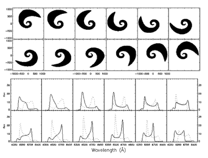
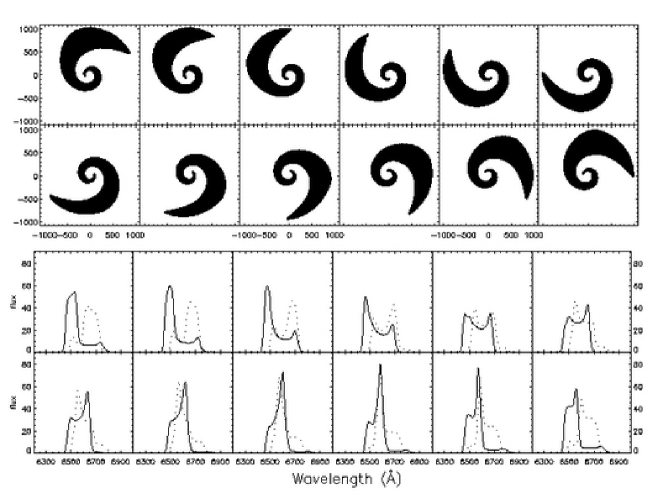
Figure 2: The images (upper panel) of the illuminated area of the disc and H$\alpha$ line profiles (lower panel) computed by our code for twist warped disc case for $i=30^{\circ},\;n_{1}=2.1\pi,\;n_{2}=3.0,\;n_{3}=10^{\circ}$, the disc zone is from $R_{\rm in}=100r_{\rm g}$ to $R_{\rm out}=1000r_{\rm g}$. The profiles from both prograde disc (black line) and retrograde disc (dotted line) are shown. The longitude of the observer $\gamma_{0}$ with respect to the coordinate system of the disc takes steps of $30^{\circ}$ from $0^{\circ}$ to $330^{\circ}$ (from top left-hand side to bottom right-hand side). All the results are smoothed by convolution with 3$\sigma$ Gaussian (corresponding to 500 $\rm km\,s^{-1}$).

Figure 3: As in Fig.3 but with $i=15^{\circ},\;n_{3}=20^{\circ}$.

Figure 4: Comparison of the H$\alpha$ line profiles generated by our code for warped disc cases with different phase amplitude (described by parameter $n_{1}$), $n_{1}=0,\;\pi,\;2\pi,\;3\pi$ (from top to bottom panels). The other parameters are: $i=30^{\circ},\;n_{2}=3.0,\;n_{3}=10^{\circ},\;R_{\rm in}=100r_{\rm g}$ and $R_{\rm out}=1200r_{\rm g}$. The longitude of the observer $\gamma_{0}$ with respect to the coordinate system of the disc varies from $0^{\circ}$ to $300^{\circ}$ with a step of $60^{\circ}$ (from left- to right-hand side).

3.1 Line profiles from twisted warping discs

We extend the numerical code developed by Wu & Wang (2007) to deal with the warped discs. The images of the illuminated area and the H$\alpha$ line profiles computed by our code for a steady-state twisted warping disc are shown in Figs 3 and 3. The disc zone is from $R_{\rm in}=100r_{\rm g}$ to $R_{\rm out}=1000r_{\rm g}$, the other parameters are $i=30^{\circ},\;n_{1}=2.1\pi,\;n_{2}=3.0,\;n_{3}=10^{\circ}$, and $i=15^{\circ},\;n_{1}=2.1\pi,\;n_{2}=3.0,\;n_{3}=20^{\circ}$, respectively. The longitude of the observer $\gamma_{0}$ with respect to the coordinate system of the disc from top left-hand side to bottom right-hand side varies from $0^{\circ}$ to $330^{\circ}$ with a step of $30^{\circ}$. The image of the illuminated portion of the disc has a shape similar to a one-armed disc. The image area of the disc being projected on the observer’s sky from the far side of the disc due to a little angle between the tilt vector $\mbox{\boldmath$l$}(R,t)$ and the line of sight significantly larger than the near parts are indicated in Figs 3 and 3. In our code, one can specify an arbitrary grid for $r$ or $\phi$. In our calculations, all the images contain $400\times 360$ pixels in this paper. The line profiles drawn in black are restricted to prograde disc models  (relative to the normal to equatorial plane or black hole spin), the effects of a retrograde disc (identical to the prograde case with a reversed spin) on the line profiles should also be taken into account if the orientations of the AGN are isotropically distributed in space, those are drawn with dotted line in the plots. The profiles from a prograde disc and its corresponding retrograde disc is close to but not exactly reflective symmetric about $v=0$ because of relativistic boosting, the gravitational redshift and the asymmetry of the disc. Note also that there are triple-peaked profiles similar to those found by observations (Veilleux & Zheng, 1991) and the obvious variation in the red/blue peak positions.

The influence of the phase amplitude (described by parameter $n_{1}$) on the line profiles for $n_{1}=0$ (twist-free), $\pi,\;2\pi,\;3\pi$ are shown in Fig. 4. The disc zone is from $R_{\rm in}=100r_{\rm g}$ to $R_{\rm out}=1200r_{\rm g}$, the other parameters are $i=30^{\circ},\;n_{2}=3.0,\;n_{3}=10^{\circ}$. The longitude of the observer $\gamma_{0}$ with respect to the coordinate system of the disc varies from $0^{\circ}$ to $300^{\circ}$ with a step of $60^{\circ}$  (from left- to right-hand side). For twist-free and low phase amplitude discs, the asymmetric as well as frequency-shifted single-peaked line profiles expected in most cases are produced. For $n_{1}>2\pi$, there is a fairly large possibility for a triple-peaked line profile. The influence of the phase amplitude on the line profiles is remarkable.

The fraction of light incident to the disc from the inner region is a function of $n_{1},n_{3}$. We calculate the fraction received by a warped disc, the results are shown in Fig. 5. The fraction reaches $27.3$ per cent for a twisted warp disc $n_{1}=2.0\pi$, $n_{2}=3.0$, $n_{3}=20^{\circ}$.

Figure 5: The fraction of light incident to the disc from the inner region as a function of $n_{1}$ or $n_{3}$. The disc zone is from $R_{\rm in}=250r_{\rm g}$ to $R_{\rm out}=1000r_{\rm g}$.

3.2 Comparison with the observations

As the first step, our main purpose in this paper is to demonstrate the effect of disc warping on the line profiles, while the detailed fitting of the observational data will be presented in a future paper. From the sample of AGN with double-peaked Balmer lines drawn from the Sloan Digital Sky Survey (SDSS) spectroscopic data set (Shan et al., in preparation), we pick up four sources with peculiar profiles: SDSS J084205.57+075925.5, SDSS J232721.96+152437.3, SDSS J094321.97+042412.0, SDSS J093653.84+533126.8. Two of them have explicit triple-peaked profiles, the others show a net shift of the emission lines to the red. These features are hard to interprete via a homogeneous, circular relativistic disc model. The SDSS spectrum of one object (SDSS J232721.96+152437.3) is dominated by starlight from the host galaxy; we subtract the starlight and the nuclear continuum with the method as described in detail in Zhou et al. (2006); The other three spectra have little starlight contamination, the nuclear continuum and the Fe II emission multiplets are modelled as described in detail in Dong et al. (2008). The FeII emission lines are apparent in J0936+5331.

The observed broad line spectrum of sources SDSS J084205.57+075925.5,
SDSS J232721.96+152437.3 both have a third peak. The line profiles (red line) calculated by our code compared with observations are shown in Figs 6 and 7. The disc zone is from $R_{\rm in}=250r_{\rm g}$ to $R_{\rm out}=1000r_{\rm g}$, and $n_{2}=3.0$ for a prograde disc case. The other parameters are: $i=13^{\circ},\;n_{1}=3.0\pi,\;n_{3}=28^{\circ},\;\gamma_{0}=95^{\circ}$ for SDSS J084205.57+075925.5, $i=10^{\circ},\;n_{1}=2.6\pi,\;n_{3}=22^{\circ},\;\gamma_{0}=88^{\circ}$ for SDSS J232721.96+152437.3, respectively. We have taken the approach that the disk-like component should be fitted by eye to as much of the peaks match as possible. While our model does not reproduce the extended wing, the peak positions and heights are reasonably in agreement with the observed profiles.

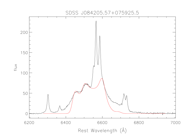
Figure 6: comparison of the H$\alpha$ line profiles computed by our code (red line) with the observation of SDSS J084205.57+075925.5. The parameters are: $i=13^{\circ},\;n_{1}=3.0\pi,\;n_{2}=3.0,\;n_{3}=28^{\circ},\;\gamma_{0}=95^{\circ}$, the disc zone is from $R_{\rm in}=250r_{\rm g}$ to $R_{\rm out}=1000r_{\rm g}$ for a prograde disc.

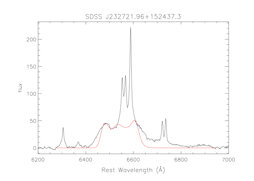
Figure 7: comparison of the H$\alpha$ line profiles computed by our code (red line) with the observation of SDSS J232721.96+152437.3. The parameters are: $i=10^{\circ},\;n_{1}=2.6\pi,\;n_{2}=3.0,\;n_{3}=22^{\circ},\;\gamma_{0}=88^{\circ}$, the disc zone is from $R_{\rm in}=250r_{\rm g}$ to $R_{\rm out}=1000r_{\rm g}$ for a prograde disc.

A retrograde disc is needed to match the line profiles with the observations for SDSS J094321.97+042412.0, J093653.84+533126.8. Fig. 8 shows the comparison between the line profiles and the observed profile for SDSS J094321.97+042412.0 with $i=17^{\circ},\;n_{1}=2.1\pi,\;n_{3}=24^{\circ},\;\gamma_{0}=202^{\circ}$. And the parameters in Fig. 9 for SDSS J093653.84+533126.8 are: $i=8^{\circ},\;n_{1}=2.1\pi,\;n_{3}=6^{\circ},\;\gamma_{0}=117^{\circ}$. The disc zone is still taken from $R_{\rm in}=250r_{\rm g}$ to $R_{\rm out}=1000r_{\rm g}$ and $n_{2}=3.0$. We see that the overall match except that in the two wings between the line profiles and the observations is good qualitatively. The deviation in two wings may, mostly due to the central point-like source adopted, diminish the contribution from the relatively inner part of the reprocessing region.

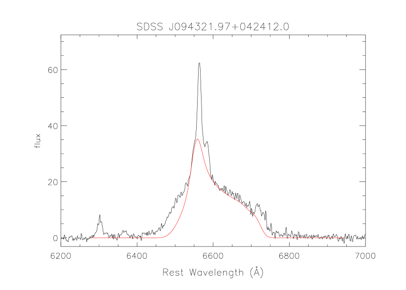
Figure 8: comparison of the H$\alpha$ line profiles computed by our code (red line) with the observation of SDSS J094321.97+042412.0. The parameters are: $i=17^{\circ},\;n_{1}=2.1\pi,\;n_{2}=3.0,\;n_{3}=24^{\circ},\;\gamma_{0}=202^{\circ}$, the disc zone is from $R_{\rm in}=250r_{\rm g}$ to $R_{\rm out}=1000r_{\rm g}$ for a retrograde disc.

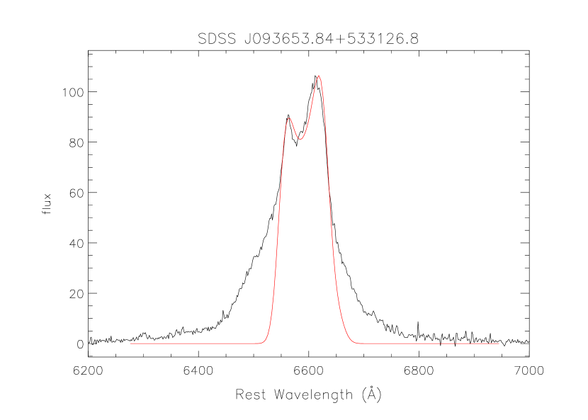
Figure 9: comparison of the H$\alpha$ line profiles computed by our code (red line) with the observation of SDSS J093653.84+533126.8. The parameters are: $i=8^{\circ},\;n_{1}=2.1\pi,\;n_{2}=3.0,\;n_{3}=6^{\circ},\;\gamma_{0}=117^{\circ}$, the disc zone is from $R_{\rm in}=250r_{\rm g}$ to $R_{\rm out}=1000r_{\rm g}$ for a retrograde disc.

The line profiles with respect to different longitude of the observer are corresponding to the observations in different times in reality. Thus the variation of the line profiles with respect to different longitude can be compared with successive observations. The images of the illuminated area and the H$\alpha$ line profiles for sources SDSS J232721.96+152437.3, SDSS J093653.84+533126.8 are shown in Figs 11 and 11. In Fig. 11 the parameters of the disc are: $i=10^{\circ},\;n_{1}=2.6\pi,\;n_{2}=3.0,\;n_{3}=22^{\circ}$, $R_{\rm in}=250r_{\rm g}$, $R_{\rm out}=1000r_{\rm g}$ for a prograde disc. The longitude of the observer $\gamma_{0}$ from top left-hand side to bottom right-hand side takes steps of $10^{\circ}$ from $30^{\circ}$ to $140^{\circ}$. A retrograde disc with $i=8^{\circ},\;n_{1}=2.1\pi,\;n_{2}=3.0,\;n_{3}=6^{\circ}$, $R_{\rm in}=250r_{\rm g}$ and $R_{\rm out}=1000r_{\rm g}$, the longitude of the observer $\gamma_{0}$ from top left-hand side to bottom right-hand side takes steps of $10^{\circ}$ from $50^{\circ}$ to $160^{\circ}$ (shown in Fig. 11). Long term monitoring of these sources should provide critical tests for the disc warping scenarios.

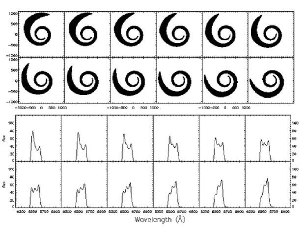
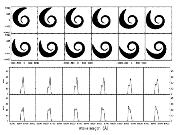
Figure 10: The images (upper panel) of the illuminated area of the disc and H$\alpha$ line profiles (lower panel) computed by our code for twist warped disc cases for $i=10^{\circ},\;n_{1}=2.6\pi,\;n_{2}=3.0,\;n_{3}=22^{\circ}$, the disc zone is from $R_{\rm in}=250r_{\rm g}$ to $R_{\rm out}=1000r_{\rm g}$ for a prograde disc. The longitude of the observer $\gamma_{0}$ with respect to the coordinate system of the disc from top left-hand side to bottom right-hand side takes steps of $10^{\circ}$ from $30^{\circ}$ to $140^{\circ}$. The variation of the line profiles with respect to different longitude corresponds to different observation time and can be compared with the future observations of source SDSS J232721.96+152437.3.

Figure 11: The images (upper panel) of the illuminated area of the disc and H$\alpha$ line profiles (lower panel) computed by our code for twist warped disc cases for $i=8^{\circ},\;n_{1}=2.1\pi,\;n_{2}=3.0,\;n_{3}=6^{\circ}$, the disc zone is from $R_{\rm in}=250r_{\rm g}$ to $R_{\rm out}=1000r_{\rm g}$ for a retrograde disc. The longitude of the observer $\gamma_{0}$ with respect to the coordinate system of the disc from top left-hand side to bottom right-hand side takes steps of $10^{\circ}$ from $50^{\circ}$ to $160^{\circ}$. The variation of the line profiles with respect to different longitude can be compared with successive observation of source SDSS J093653.84+533126.8.

4 Summary

We compute the reprocessing emission-line profiles from a warped relativistic accretion disc around a central black hole by including all relativistic effects. A parametrized disc model is used to obtain an insight into the impact of disc warping on the double-peaked Balmer emission-line profiles. For simplicity, we assumed that the disc is illuminated by a point-like central source, which is a good approximation, the line emissivity is proportional to the continuum light intercepted by the accretion disc, and line emission is isotropic. We find the following.

1. For twist-free or low phase amplitude (described by $n_{1}$) warped disc, the asymmetrical and frequency-shifted single-peaked line profiles as expected are produced in most cases. The rarity of such sources suggests that a warping disc is usually twisted.

2. The flux ratio of the blue peak to red one becoming less than unity can be predicted by a twisted warp disc with high phase amplitude. The phase amplitude has a significant influence on the line profiles.

3. A third peak and the variation in blue/red peak position which have been found by observations (Veilleux & Zheng, 1991; Strateva et al., 2003) are produced in our model.

4. The influence from retrograde disc on line profiles has a inverse effect compared with a prograde one.

5. The fraction of the radiation incident to the outer disc from the inner part can be enhanced by disc warping. The results are shown in Fig. 5.

We showed that warped disc model is flexible enough to reproduce a variety of line profiles including triplet-peaked line profiles, or double peaked profiles with additional plateaus in the line wing as observed in the SDSS spectra of some AGN, while the models have the same number of free parameters as eccentric disc models. While we leave the detailed fit to a future paper, the essential characteristics in the line profiles is in good agreement with observed line profiles. Future monitoring of line profile variability in these triplet sources can provide a critical test of the warped disc model.

5 acknowledgments

We would like to thank the anonymous referee for his/her helpful suggestions and comments which improve and clarify our paper.

References

- Armitage & Natarajan (1999) Armitage P. J., Natarajan P., 1999, ApJ, 525, 909
- Bardeen & Petterson (1975) Bardeen J. M., Petterson J. A., 1975, ApJ, 195, L65
- Bardeen et al. (1972) Bardeen J. M., Press W. H., Teukolsky S. A., 1972, ApJ, 178, 347
- Bachev (1999) Bachev R., 1999, A&A, 348, 71
- Begelman, Blandford & Rees (1980) Begelman M. C., Blandford R. D., Rees M. J., 1980, Nature, 287, 307
- Bian et al. (2007) Bian W.-H., Chen Y.-M., Gu Q.-S., Wang J.-M., 2007, ApJ, 668, 721
- Čadež et al. (2003) Čadež A., Brajnik M., Gomboc A., Calvani M., Fanton C., 2003, A&A, 403, 29
- Čadež et al. (1998) Čadež A., Fanton C., Calvani M., 1998, New Astronomy, 3, 647
- Caproni et al. (2007) Caproni A., Abraham Z. Livio M., Mosquera Cuesta H. J., 2007, MNRAS, 379,135
- Cao & Wang (2006) Cao X., Wang T. G., 2006, ApJ, 652, 112
- Carter (1968) Carter B., 1968, Phys. Rev., 174, 1559
- Chakrabarti & Wiita (1993) Chakrabarti S., Wiita P. J., 1993, ApJ, 411, 602
- Chakrabarti & Wiita (1994) Chakrabarti S., Wiita P. J., 1994, ApJ, 434, 518
- Chen & Halpern (1989) Chen K., Halpern J. P., 1989, ApJ, 344, 115
- Chen et al. (1989) Chen K. , Halpern J. P., Filippenko A. V., 1989, ApJ, 339, 742
- Cunningham (1975) Cunningham C. T., 1975, ApJ, 202, 788
- Cunningham & Bardeen (1973) Cunningham C. T., Bardeen J. M., 1973, ApJ, 183, 237
- Dong et al. (2008) Dong X., Wang T., Wang J., Yuan W., Zhou H., Dai H., Zhang K., 2008, MNRAS, 383, 581
- Eracleous & Halpern (1994) Eracleous M., Halpern J. P., 1994, ApJS, 90, 1
- Eracleous & Halpern (2003) Eracleous M., Halpern J. P., 2003, ApJ, 599, 886
- Eracleous et al. (1995) Eracleous M. , Livio M. , Halpern J. P., Storchi-Bergmann T., 1995, ApJ, 438, 610
- Eracleous et al. (1997) Eracleous M., Halpern J. P., Gilbert A. M., Newman J.A., Filippenko A. V., 1997, ApJ, 490, 21
- Gezari et al. (2007) Gezari S., Halpern J. P., Eracleous M., 2007, ApJS, 169, 167
- Gaskell (1996) Gaskell C. M., 1996, ApJ, 464, 107
- Hartnoll & Blackman (2000) Hartnoll S. A., Blackman E. G., 2000, MNRAS, 317, 880
- Herrnstein et al. (2005) Herrnstein J. R., Moran J. M., Greenhill L. J., Trotter A., 2005, ApJ, 629 719
- Kumar & Pringle (1985) Kumar S., Pringle J. E., 1985, MNRAS, 213, 435.
- Lai (1999) Lai, D. 1999, ApJ, 524, 1030
- Lai (2003) Lai, D. 2003, ApJ, 591, L119
- Larwood et al. (1996) Larwood J. D., Nelson R. P., Papaloizou J. C. B., Terquem C., 1996, MNRAS, 282, 597
- Lu & Yu (2001) Lu Y., Yu Q., 2001, ApJ, 561, 660
- Maloney, Begelman & Pringle (1996) Maloney P. R., Begelman M. C., Pringle J. E., 1996, ApJ, 472, 582
- Maloney & Begelman (1997) Maloney P. R., Begelman M. C., 1997, ApJ, 491, L43
- Maloney, Begelman & Nowak (1998) Maloney P. R., Begelman M. C., Nowak M. A., 1998, ApJ, 504, 77
- Miller & Peterson (1990) Miller J. S., Peterson B. M., 1990, ApJ, 361, 98
- Nayakshin (2005) Nayakshin S. , 2005, MNRAS, 359, 545
- Nelson & Papaloizou (1999) Nelson R. P., Papaloizou J. C. B., 1999, MNRAS, 309, 929
- Nelson & Papaloizou (2000) Nelson R. P., Papaloizou J. C. B., 2000, MNRAS, 315, 570
- Ogilvie (1999) Ogilvie G. I., 1999, MNRAS, 304, 557
- Papaloizou & Lin (1995) Papaloizou J. C. B., Lin D. N. C., 1995, ApJ, 438, 841
- Papaloizou & Pringle (1983) Papaloizou J. C. B., Pringle J. E., 1983, MNRAS, 202, 1181
- Pfeiffer & Lai (2004) Pfeiffer H. P., Lai D., 2004, ApJ, 604, 766
- Press et al. (1992) Press W. H., Teukolsky S. A., Vetterling W. T., Flannery B. P., 1992, Numerical Recipes. Cambridge University Press, Cambridge
- Pringle (1996) Pringle J. E., 1996, MNRAS, 281, 357
- Pringle (1997) Pringle J. E., 1997, MNRAS, 292, 136
- Storchi-Bergmann et al. (1997) Storchi-Bergmann T. , Eracleous M., Ruiz M. T. , Livio M. , Wilson A. S. , FIlippenko A. V., 1997, ApJ, 489, 87
- Strateva et al. (2003) Strateva I. V. et al., 2003, AJ, 126, 1720
- Terquem & Bertout (1993) Terquem C., Bertout C., 1993, A&A, 274, 291
- Terquem & Bertout (1996) Terquem C., Bertout C., 1996, A&A, 279, 415
- Veilleux & Zheng (1991) Veilleux S., Zheng W., 1991, ApJ, 377, 89
- Viergutz (1993) Viergutz S. U., 1993, A&A, 272, 355
- Wang et al. (2005) Wang T.-G., Dong X.-B., Zhang X.-G., Zhou H.-Y., Wang J.-X., Lu Y.-J, 2005, ApJ, 625, L35
- Wilkins (1972) Wilkins D. C., 1972, Phys. Rev. D5, 814
- Wu & Wang (2007) Wu S.-M., Wang T.-G., 2007, MNRAS, 378, 841
- Zhang, Dultzin-Hacyan & Wang (2007a) Zhang X. -G., Dultzin-Hacyan D., Wang T.-G., 2007, MNRAS, 376, 1335
- Zhang, Dultzin-Hacyan & Wang (2007b) Zhang X. -G., Dultzin-Hacyan D., Wang T.-G., 2007, MNRAS, 377, 1215
- Zheng, Sulentic & Binette (1990) Zheng W., Sulentic J. W., Binette L., 1990, ApJ, 365, 115
- Zhou et al. (2006) Zhou H., Wang T., Yuan W., Lu H., Dong X., Wang J., Lu Y., 2006, ApJS, 166, 128