Spectral signature of a free pulsar wind in the gamma-ray binaries LS 5039 and LSI +61$\degr$303

Abstract

Context. LS 5039 and LSI +61$\degr$303 are two binaries that have been detected in the TeV energy domain. These binaries are composed of a massive star and a compact object, possibly a young pulsar. The gamma-ray emission would be due to particle acceleration at the collision site between the relativistic pulsar wind and the stellar wind of the massive star. Part of the emission may also originate from inverse Compton scattering of stellar photons on the unshocked (free) pulsar wind.

Aims. The purpose of this work is to constrain the bulk Lorentz factor of the pulsar wind and the shock geometry in the compact pulsar wind nebula scenario for LS 5039 and LSI +61$\degr$303 by computing the unshocked wind emission and comparing it to observations.

Methods. Anisotropic inverse Compton losses equations are derived and applied to the free pulsar wind in binaries. The unshocked wind spectra seen by the observer are calculated taking into account the $\gamma-\gamma$ absorption and the shock geometry.

Results. A pulsar wind composed of monoenergetic pairs produces a typical sharp peak at an energy which depends on the bulk Lorentz factor and whose amplitude depends on the size of the emitting region. This emission from the free pulsar wind is found to be strong and difficult to avoid in LS 5039 and LSI +61$\degr$303.

Conclusions. If the particles in the pulsar are monoenergetic then the observations constrain their energy to roughly 10-100 GeV. For more complex particle distributions, the free pulsar wind emission will be difficult to distinguish from the shocked pulsar wind emission.

1 Introduction

Pulsars are fast rotating neutron stars that contain a large amount of rotational energy. A significant fraction of this energy is carried away by an ultra-relativistic wind of electrons/positrons pairs and possibly ions (see Kirk et al. 2007 for a recent review). In the classical model of the Crab nebula (Rees & Gunn 1974; Kennel & Coroniti 1984), the pulsar wind is isotropic, radial and monoenergetic with a bulk Lorentz factor $\gamma_{0}\sim 10^{6}$ far from the light cylinder where the wind is kinetic energy-dominated ($\sigma\ll 1$). The cold relativistic wind expands freely until the ram pressure is balanced by the surrounding medium at the standoff distance $\rm{R_{s}}$. In the termination shock region, the pairs are accelerated and their pitch angle to the magnetic field are randomized, producing an intense synchrotron source. Moreover, the inverse Compton scattering of the relativistic electrons on soft photons produces high energy (HE, GeV domain) and very high energy (VHE, TeV domain) gamma-rays.

The shocked pulsar wind is thought to be responsible for most of the emitted radiation and gives clues about the properties of this region. However, our knowledge of the unshocked pulsar wind region is limited and based on theoretical statements. If the magnetic field is frozen into the pair plasma as it is usually assumed, there is no synchrotron radiation from the unshocked wind. Nevertheless, nothing prevents inverse Compton scattering of soft photons onto the cold ultra-relativistic pairs from occuring. The pulsar wind nebula (PWN) emission has two components: radiation from the shocked and the unshocked regions.

Bogovalov & Aharonian (2000) investigated the inverse Compton emission from the region upstream the termination shock of the Crab pulsar. Comparisons between calculated and measured fluxes put limits on the parameters of the wind, in particular the size of the kinetic energy dominated region. Ball & Kirk (2000) investigated emission from an unshocked freely expanding wind with no termination shock in compact binaries. They computed spectra and light curves in the gamma-ray binary PSR B1259-63, a system with a 48 ms pulsar and a Be star in a highly eccentric orbit. The resulting gamma-ray emission is a line-like spectrum.

In addition to PSR B1259-63, two other binaries have been firmly confirmed as gamma-ray sources: LS 5039 (Aharonian et al. 2005) and LSI +61$\degr$303 (Albert et al. 2006). They are composed of a massive O or Be star and a compact object in an eccentric orbit. The presence of a young pulsar was detected only in PSR B1259-63 (Johnston et al. 1992). Radio pulses are detectable but vanish near periastron, probably due to free-free absorption and interaction with the Be disk wind. The compact PWN scenario is most probably at work in this system and investigations were carried out to model high and very high energy radiation (Kirk et al. 1999; Sierpowska & Bednarek 2005; Khangulyan et al. 2007; Sierpowska-Bartosik & Bednarek 2008). In LS 5039 and LSI +61$\degr$303  the nature of the compact object is still controversial but spectral and temporal similarities with PSR B1259-63 argue in favor of the compact pulsar wind nebula scenario (Dubus 2006b). The VHE radiation would therefore be produced by the interaction between the pulsar wind and the stellar companion wind. The massive star provides a huge density of seed photons for inverse Compton scattering with the ultra-relativistic pairs from the pulsar wind. Because of the relative position of the compact object, the companion star and the observer, the Compton emission is modulated on the orbital period. The vicinity of a massive star is an opportunity to probe the pulsar wind at small scales.

The component of the shocked pulsar wind was computed in Dubus et al. (2008) for LS 5039 and limits on the electron distribution, the pulsar luminosity and the magnetic field at the termination shock were derived. Sierpowska-Bartosik & Torres (2008) calculated the VHE emission in LS 5039 as well, assuming a power law injection spectrum for the pairs in the unshocked pulsar wind and pair cascading. In this paper, we investigate the anisotropic inverse Compton scattering of stellar photons on the unshocked pulsar wind within the compact PWN scenario for LS 5039 and LSI +61$\degr$303. Because of their tight orbits, the photon density is higher than in the Crab pulsar and PSR B1259-63. A more intense gamma-ray signal from the unshocked pulsar wind is expected. The main purpose of this work is to constrain the bulk Lorentz factor $\gamma_{0}$ of the pairs and the shock geometry. The next section presents the method and the main equations used in order to compute spectra in gamma-ray binaries. Section 3 describes and shows the expected spectra for LS 5039 and LSI +61$\degr$303 with different parameters. Section 4 discusses the spectral signature from the unshocked pulsar wind.

2 Anisotropic Compton losses in $\gamma$-binaries

2.1 The cooling of pairs

An electron of energy $\rm{E_{e}}=\gamma_{e}m_{e}c^{2}$ in a given soft photon field of density $n_{0}$ ph $\rm{cm}^{-3}$ cools down through inverse Compton scattering (here the term ‘electrons’ refers indifferently to electrons and positrons). The power lost by the electron is given by (Jones 1965; Blumenthal & Gould 1970)

$$-\frac{dE_{e}}{dt}=\int^{\epsilon_{+}}_{\epsilon_{-}}\left(\epsilon_{1}-\epsilon_{0}\right)n_{0}\frac{dN}{dtd\epsilon_{1}}d\epsilon_{1}$$ (1)

where $\epsilon_{0}$ is the incoming soft photon energy, $\epsilon_{1}$ the scattered photon energy and dN/dtd$\epsilon_{1}$ is the Compton kernel. $\epsilon_{\pm}$ boundaries are fixed by the relativistic kinematics of inverse Compton scattering. The cooling of the pairs $\rm{e^{+}/e^{-}}$ depends on the angular distribution and spectrum of the incoming photon field. In the simple case of a monoenergetic and unidirectional beam of photons in the Thomson limit, the calculation of the Compton energy loss per electron is

$$-\frac{dE_{e}}{dt}=\sigma_{T}cn_{0}\epsilon_{0}\left(1-\beta\mu_{0}\right)\left[\left(1-\beta\mu_{0}\right)\gamma^{2}_{e}-1\right]$$ (2)

where $\sigma_{T}$ is the Thomson cross section, $\mu_{0}=\cos\theta_{0}$ and $\theta_{0}$ the angle between the incoming photon and the direction of the electron motion. This calculation is done using the Compton kernel calculated by Fargion et al. (1997). In the Thomson limit, the cooling of the electron follow a $\gamma_{e}^{2}$ power law and has a strong angular dependance. In a more general way and for $\gamma_{e}\gg 1$, the power lost per electron is calculated with the kernel derived in Dubus et al. (2008) Eq. (A.6).

2.2 Compton cooling of the free pulsar wind

The pulsar is considered as a point-like source of monoenergetic and radially expanding wind of relativistic pairs $e^{+}/e^{-}$. The pulsar wind momentum is assumed to be entirely carried away by the pairs. The companion star, with a typical luminosity of $10^{38}-10^{39}$ ergs $\rm{s^{-1}}$, provides seeds photons for inverse Compton scattering onto the radially expanding electrons from the pulsar. The electrons see a highly anisotropic photon field. Inverse Compton efficiency has a strong dependence on $\theta_{0}$ as seen in Eq. (2). Depending of the relative position and direction motion of the electron with respect to the incoming photons direction, the cooling of the wind is anisotropic as well. Figure 1 sketches the geometry considered in the binary system to perform calculations.

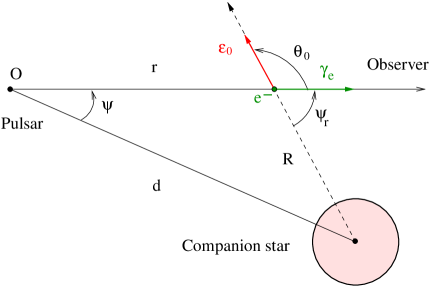
Figure 1: Geometry of the binary system. Electrons of Lorentz factor $\gamma_{e}$ are radially moving away at a distance r from the pulsar and R from the companion star. The angle $\psi$ quantifies the relative position between the pulsar, the companion star and the observer. $\psi_{r}$ measures the angle between the electron direction of motion and the line joining the companion star center to the electron position through its motion to the observer.

For ultra-relativistic electrons , the radial dependence of the electron Lorentz factor $\gamma_{e}(r)$ for a given viewing angle is obtained by solving the first order differential equation Eq. (1). Chernyakova & Illarionov (1999) found an analytical solution in the Thomson limit and Ball & Kirk (2000) derived a solution in the general case using the Jones (1965) results for a point-like and monoenergetic star with $\gamma_{e}\gg 1$. In this approximation, the density of photons is $L_{\star}/(4\pi cR^{2}\bar{\epsilon}_{0})$ ph $\rm{cm^{-3}}$, where $L_{\star}$ is the star luminosity and $\bar{\epsilon}_{0}=2.7kT_{\star}$ the average energy photon from the star. The differential equation is then

$$\frac{d\gamma_{e}}{dr}=-\frac{1}{m_{e}c^{3}}\frac{L_{\star}}{4\pi cR^{2}}\int_{\epsilon_{-}}^{\epsilon_{+}}\left(\frac{\epsilon_{1}-\bar{\epsilon}_{0}}{\bar{\epsilon}_{0}}\right)\frac{dN}{dtd\epsilon_{1}}d\epsilon_{1}$$ (3)

where $R^{2}=d^{2}+r^{2}-2rd\cos\psi$. Calculations beyond the monoenergetic and point-like star approximation require two extra integrations, one over the star spectrum and the other onto the angular distribution of the incoming photons due to the finite size of the star. The complete differential equation is then given by

$$\frac{d\gamma_{e}}{dr}=-\frac{1}{m_{e}c^{3}}\iiint\left(\epsilon_{1}-\epsilon_{0}\right)n_{0}\frac{dN}{dtd\epsilon_{1}}d\epsilon_{1}d\epsilon_{0}d\Omega_{0}.$$ (4)

For a blackbody of temperature $T_{\star}$ and a spherical star of radius $R_{\star}$, the incoming photon density $n_{0}$ is given by Eq. (13) in Dubus et al. (2008). It is more convenient to compute the calculation of the Lorentz factor as a function of $\psi_{r}$ rather than $r$ (see Fig. 1). These two variables are related through the relation

$$r=d\cos\psi\left(1-\frac{\tan\psi}{\tan\psi_{r}}\right),\hskip 5.69054ptr\in[0,+\infty],\hskip 5.69054pt\psi_{r}\in[\psi,\pi].$$ (5)

Figure 2 presents the numerical computed output solution $\gamma(\psi_{r})$ applied to LS 5039 with an inclination of $i=60\degr$ for a neutron star where the viewing angle varies between $\pi/2-i=30\degr$ and $\pi/2+i=150\degr$. Here, the wind is assumed to have an injection Lorentz factor $\gamma(\psi_{r}(0))=\gamma_{0}=10^{5}$ and to continue unimpeded to infinity (i.e. it is not contained by the stellar wind).

Figure 2: Compton cooling of a monoenergetic, free pulsar wind with $\gamma_{0}=10^{5}$, $d=2R_{\star}$ ($T_{\star}=39$ 000 K, $R_{\star}=9.3$ $R_{\odot}$). The different curves show the dependence with the viewing angle $\psi$ on the cooling. $\psi$ varies between $30\degr$ (bottom) and $150\degr$ (top) if $i=60\degr$. Each curve shows the evolution of the Lorentz factor $\gamma$ with $\psi_{r}$ as the electron moves along the line of sight. $\psi_{r}$ is related to $r$ by Eq. (5) so that $\psi_{r}=\psi$ at $r=0$ and $\psi_{r}=\pi$ for $r=+\infty$. The calculation was carried out for a blackbody point like star (solid line) and taking into account the finite size of the star (dashed line).

For small viewing angles $\psi$, the cooling of the wind is very efficient because the collision electron/photon is almost head-on and the electrons are moving in the direction of the star where the photon density increases. For viewing angles $\psi\ga\pi/2$, the cooling of the pairs is limited. In all cases, most of the cooling occurs at $\psi_{r}\sim\psi$. For $\psi_{r}\ga\pi/2$, the electron is moving away from the star and the scattering angle become small leading to a decrease in the wind energy loss. A comparison of Compton cooling between the point-like and finite size star is shown in Fig. 2. The effects of the finite size of the star are significant in two cases. The impact of the finite size of the star is important if the observer is within the cone defined by the star and the electron at apex (see Dubus et al. 2008 for more details). For viewing angles $\psi\la\arcsin(R_{\star}/d)$, the cooling is less efficient whereas for $\psi\ga\pi-\arcsin(R_{\star}/d)$ it is more efficient as it can be seen in the two extreme value of $\psi$ in figure 2. The other situation occurs when the electrons travel close to the companion star surface, for $\psi\la\pi/2$ and $\psi_{r}\ga\pi/2$. In that case the angular distribution of the stellar photons is broad and close head-on scatterings are possible, leading to more efficient cooling compared with a point-like star. Nevertheless, these effects remain small for LS 5039 and LSI +61$\degr$303 and will be neglected in the following spectral calculations.

Figure 3: Computed inverse Compton spectrum from the unshocked pulsar wind in LS 5039 and its dependence with the emitting region size $R_{s}$. The pulsar wind has $\gamma_{0}=10^{5}$, $L_{p}=10^{36}$ erg $\rm{s^{-1}}$ and the star is a point-like blackbody. Spectra are calculated at the superior (left) and inferior (right) conjunctions for different standoff distances $R_{s}=10^{10}$ (bottom), $3$ $10^{10}$, $10^{11}$, $3$ $10^{11}$ cm and $+\infty$ (dashed line).

2.3 Unshocked pulsar wind spectra

The number of scattered photons per unit of time, energy and solid angle depends on three contributions: the density of the incoming photons, the density of target electrons and the number of scattered photons per electron. The pulsar wind of luminosity $L_{p}$ is assumed isotropic and monoenergetic, composed only of pairs and with a negligible magnetic energy density ($\sigma\ll 1$). The electrons density ($\rm{e}^{-}$ $\rm{cm}^{-3}$ $\rm{erg}^{-1}$) is then proportional to $1/r^{2}$ if pair production is neglected. Here, the interesting quantity for spectral calculations is the number of electrons per unit of solid angle, energy and length, which is $r^{2}$ time the electrons density so that (Ball & Kirk 2000)

$$\frac{dN_{e}}{d\Omega_{e}d\gamma dr}=\frac{L_{p}}{4\pi c\beta_{0}\gamma_{0}m_{e}c^{2}}\delta\left(\gamma-\gamma_{e}(r)\right),$$ (6)

with $\delta$ the Dirac distribution. In deep Klein-Nishina regime, spectral broadening is expected because the continuous energy loss prescription fails ($\Delta E_{e}\sim E_{e}$). The complete kinetic equation must be used in order to describe accurately the electrons dynamics (see Blumenthal & Gould 1970 Eq. (5.7)). However, the $\delta$ approximation used here is reasonably good (Zdziarski 1989). The case of an anisotropic pulsar wind is discussed in §4. In the following, the pulsar wind will therefore be assumed to follow Eq. (6). Heating of the pulsar wind by the radiative drag is neglected (Ball & Kirk 2000).

In order to compute spectra, the emitted photons are supposed to be entirely scattered in the direction of the electron motion. Because of the ultra-relativistic motion of the electrons, most of the emission is within a cone of aperture angle of the order of $1/\gamma_{e}\ll 1$. In this classical approximation, the spectrum seen by the observer is the superposition of the contributions from the electrons along the line of sight pulsar-observer in the solid angle $d\Omega_{e}$. The spectrum seen by the observer is obtained with the following formula

$$\frac{dN_{tot}}{dtd\epsilon_{1}d\Omega_{e}}=\iiiint n_{0}\frac{dN}{dtd\epsilon_{1}}e^{-\tau_{\gamma\gamma}}\frac{dN_{e}}{d\Omega_{e}d\gamma dr}d\gamma d\epsilon_{0}drd\Omega_{0}$$ (7)

where $\tau_{\gamma\gamma}$ takes into account the absorption of gamma-rays due to pair production with soft photons from the companion star and is calculated following Dubus (2006a).

2.4 The compact PWN geometry

The collision of the relativistic wind from the pulsar and the non-relativistic wind from the massive star produces two termination shock regions separated by a contact discontinuity (see Fig. 4). The geometry of the shock fronts are governed by the ratio of the flux wind momentum quantified by $\eta$ and defined as (e.g. Stevens et al. 1992; Eichler & Usov 1993)

$$\eta=\frac{L_{p}}{c\dot{M}_{w}v_{\infty}}$$ (8)

where $\dot{M}_{w}$ is the mass loss rate and $v_{\infty}$ the stellar wind speed of the O/Be star. For two spherical winds, the standoff distance point $R_{s}$ depends on $\eta$ and on the orbital separation $d$

$$R_{s}=\frac{\sqrt{\eta}}{1+\sqrt{\eta}}d.$$ (9)

Bogovalov et al. (2008) have investigated the collision between the pulsar wind and the stellar wind in the binary PSR B1259-63, with a relativistic code and an isotropic pulsar wind in the hydrodynamical limit. They obtained the geometry for the relativistic and nonrelativistic shock fronts and the contact discontinuity. They find that the collision between the two winds produces an unclosed pulsar wind termination shock (in the backward facing direction) for $\eta>1.25\hskip 2.84526pt10^{-2}$.

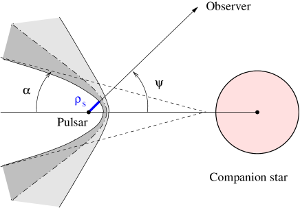
Figure 4: Shock geometry considered for the wind collision. For $\eta>1.25$ $10^{-2}$, the pulsar wind region remains open with an asymptotic half-opening angle $\alpha$. The dark region is the shocked relativistic pulsar wind and the light region is the shocked non-relativistic stellar wind, separated by a contact discontinuity (dot-dashed line). The size of the emitting zone seen by the observer $\rho_{s}$ depends on the viewing angle $\psi$.

The size of the emitting region depends on the shock geometry and the viewing angle, which can therefore have a major impact on the emitted spectra. Ball & Dodd (2001) computed spectra from the unshocked pulsar wind in PSR B1259-63 for an hyperbolic shock front terminated close to the pulsar. They found a decrease in the spectra fluxes and a decrease in the light curve asymmetry and flux particularly near periastron compared with the spectra computed by Ball & Kirk (2000).

Figure 3 presents computed spectra, ignoring $\gamma\gamma$ absorption at this stage, applied to LS 5039 at the superior and inferior conjunctions for different standoff distances $R_{s}$ and a pulsar wind with $\gamma_{0}=10^{5}$. At the superior conjunction where $\psi=30\degr$, the Compton cooling of the wind is efficient. The broadness in energy of the radiated spectra is related to the size of the unshocked pulsar wind region. For small standoff distances $R_{s}\ll d$, spectra are truncated and sharp because the termination shock region is very close to the pulsar, so that the pairs do not have time to radiate before reaching the shock. For $R_{s}\ga d$, the free pulsar wind region is extended and emission from cooled electrons starts contributing to the low energy tail in the scattered spectrum. The amplitude of the spectrum reaches a maximum when the injected particles can cool efficiently before reaching the shock. The spectral luminosity is then set by the injected power and is not affected anymore by the size of the emitting zone. At the inferior conjunction where $\psi=150\degr$, the cooling is less efficient and most of the emission occurs close to the pulsar where the photon density and $\theta_{0}$ are greater, regardless of the size of the emitting region. The radiated flux then depends linearly on $R_{s}$. A complete investigation is presented in the next section where absorption and spectra along the orbit are computed and applied to LS 5039 and LSI +61$\degr$303, ignoring pair cascading.

3 Spectral signature of a monoenergetic pulsar wind in LS 5039 and LSI +61$\degr$303

In the following sections, the emission expected by the unshocked pulsar wind in LS 5039 and LSI +61$\degr$303 is compared with measured fluxes. Because spectra depends on the shock geometry and the injection Lorentz factor, spectra are calculated for various values of the two free parameters $\eta$ and $\gamma_{0}$.

3.1 LS 5039

Figure 5: Total radiated power by the unshocked pulsar wind $P_{rad}$ in LS 5039 as a function of $\gamma_{0}$. $P_{rad}$ is computed at periastron for $\eta=10^{-3}$ (solid line), 2 $10^{-2}$ (dotted line), $10^{-1}$ (dashed line) and with no termination shock (dotted-dashed line).

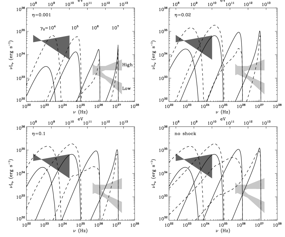
Figure 6: Spectral signature from the unshocked pulsar wind expected in LS 5039 and dependence with $\gamma_{0}$ and $\eta$. Spectra are averaged on the orbital phases corresponding to the HESS ‘high state’ (solid line, $0.45<\phi<0.9$, with $\phi\equiv 0$ at periastron) and ‘low state’ (dashed line, $\phi<0.45$ or $\phi>0.9$). The spectra are compared with EGRET (dark bowtie) and HESS (light bowties) observations, adopting a distance of 2.5 kpc. In the top left panel, $\eta=10^{-3}$ the shock is closed and the unshocked pulsar wind is assumed spherical. For $\eta=2$ $10^{-2}$ (top right panel) and $\eta=0.1$ (bottom left panel) the shock is open with half-opening angles $\alpha\sim 2\degr$ and $\alpha\sim 30\degr$ respectively. The bottom right panel shows the extreme case with no termination shock.

The companion star and the pulsar winds are assumed isotropic and purely radial. The orbital parameters are those measured by Casares et al. (2005b) as used in Dubus et al. (2008).

Figure 5 gives the total power radiated by the electrons in the unshocked pulsar wind as a function of $\gamma_{0}$ at periastron. Here, the shock front is assumed spherical of radius $R_{s}$. A maximum of efficiency is observed at about $\gamma_{0}\sim 10^{5}$ which corresponds to the transition between the Thomson and Klein-Nishina regimes where the Compton timescale is shortest (Dubus 2006b). The fraction of the pulsar wind power radiated at periastron depends strongly on $R_{s}$. It is about $20\%$ for $\eta=10^{-3}$ and can reach $70\%$ for $\eta=0.1$. Hence, most of the spindown energy can be radiated directly by the unshocked pulsar wind.

Figure 6 presents computed spectra averaged along the orbit for different shock geometry and Lorentz factor with a pulsar spindown luminosity of $L_{p}=10^{36}$ erg $\rm{s^{-1}}$. The relativistic shock front is described by an hyperbolic equation. The hyperbola apex is set by Eq. (9) and the asymptotic half-opening angle $\alpha$ is taken from Eq. (27) in Bogovalov et al. (2008), both parameters depending only on $\eta$. Figure 4 sketches the shock morphology for $1.25$ $10^{-2}<\eta<1$ and presents the different shock fronts expected. The twist due to the orbital motion is ignored since most of the emission occurs in the vicinity of the pulsar. The size of the emitting zone $\rho_{s}$ seen by the observer is thus set for any given viewing angle $\psi$. Note that it is always greater than $R_{s}$. The remaining free parameter $\gamma_{0}$ is chosen independently between $10^{4}$ and $10^{7}$.

Computed spectra predict the presence of a narrow peak in the spectral energy distribution due to the presence of the free pulsar wind. The luminosity of this narrow peak can be comparable to or greater than the measured fluxes by EGRET and HESS (Hartman et al. 1999; Aharonian et al. 2006). For $\eta=10^{-3}$, the pulsar wind termination shock is closed and the unshocked wind emission zone is small. For $\eta=0.02$ and $\eta=0.1$ the line spectra are well above both the limits imposed by the HESS observations. The extreme case with no termination shock shows little differences with the case where $\eta=0.1$. Spectroscopic observations of LS 5039 constrains the O star wind parameters to $\dot{M}_{w}\sim 10^{-7}$ $M_{\odot}$ $\rm{yr}^{-1}$ and $v_{\infty}\sim 2400$ km $\rm{s}^{-1}$ (McSwain et al. 2004). Assuming $L_{p}=10^{36}$ erg $\rm{s}^{-1}$ then gives $\eta\sim 2$ $10^{-2}$ (top right panel of Fig. 6) or $R_{s}\approx 2$ $10^{11}$ cm as in (Dubus 2006b). In this case, almost half of the pulsar wind energy is lost to inverse Compton scattering before the shock is reached (Fig. 5). This is an upper limit since the reduced pulsar wind luminosity would bring the shock location closer to the pulsar than estimated from Eq. (9). HESS observations already rule out a monoenergetic pulsar wind with $\gamma_{0}=10^{6}$ or $10^{7}$ and $L_{p}=10^{36}$ erg $\rm{s^{-1}}$ as this would produce a large component easily seen at all orbital phases (see Fig. 5 in Dubus et al. 2008). The EGRET observations probably also already rule out values of $\gamma\leq 10^{5}$.

3.2 LSI +61$\degr$303

In this system the stellar wind from the companion star is assumed to be composed of a slow dense equatorial disk and a fast isotropic polar wind. The stellar wind may be clumpy and Zdziarski et al. (2008) have proposed a model of the high-energy emission from LSI +61$\degr$303 that entails a mix between the stellar and the pulsar wind. The orbital parameters are those measured by Casares et al. (2005a) (new orbital parameters were recently measured by Grundstrom et al. 2007).

Computed spectra applied to LSI +61$\degr$303 and averaged over the orbit to compare with EGRET and MAGIC luminosities (Hartman et al. 1999; Albert et al. 2006) are presented in Fig. 8. New data were recently reported by the MAGIC collaboration (Albert et al. 2008). They confirmed the measurements of the first observational compaign and found a periodicity in the gamma-ray flux close to the orbital period. The pulsar spindown luminosity is set to $L_{p}=10^{36}$ erg $\rm{s}^{-1}$ and the injected Lorentz factor to $10^{4}$, $10^{5}$, $10^{6}$ and $10^{7}$ as for LS 5039. There is more uncertainty in $\eta$ because of the complexity of the stellar wind. The polar outflow is usually modelled with $\dot{M}_{w}=10^{-8}$ $M_{\odot}$ $\rm{yr}^{-1}$ and $v_{\infty}=2000$ km $\rm{s}^{-1}$ (Waters et al. 1988) leading to $\eta\sim 0.2-0.3$. Concerning the slow dense equatorial disk, the mass flux is typically one hundred times greater than the polar wind and the terminal velocity is a few hundred km $s^{-1}$ giving $\eta$ compatible with $\sim 10^{-3}-10^{-2}$.

The overall behaviour is similar to LS 5039. The spectral luminosities and the total power radiated by the unshocked pulsar wind (Fig. 7) are lower in LSI +61$\degr$303 than LS 5039 because the compact object is more distant to its companion star and the latter has a lower luminosity, leading to a decrease in the density of seed photons for inverse Compton scattering. If $\eta=10^{-3}$, no constrains on $\gamma_{0}$ can be formulated as the spectrum is always below the observational limits. For larger values of $\eta$, the very high energy observations constrain $\gamma_{0}$ to below $10^{6}$, assuming the pulsar wind is monoenergetic. Spectra were computed for $\eta=0.53$ with $\dot{M}_{w}=10^{-8}$ $M_{\odot}$ $\rm{yr}^{-1}$ and $v_{\infty}=1000$ km $\rm{s}^{-1}$ as used by Romero et al. (2007). In this case, the spectra are close to the freely propagating pulsar wind. The EGRET luminosity is slightly overestimated for $\gamma_{0}\leq 10^{5}$ when $\eta=0.53$.

Figure 7: Total radiated power by the unshocked pulsar wind $P_{rad}$ in LSI +61$\degr$303 as a function of $\gamma_{0}$. $P_{rad}$ is computed at periastron for $\eta=10^{-3}$ (solid line), 2 $10^{-2}$ (dotted line), 0.53 (dashed line) and with no termination shock (dotted-dashed line).

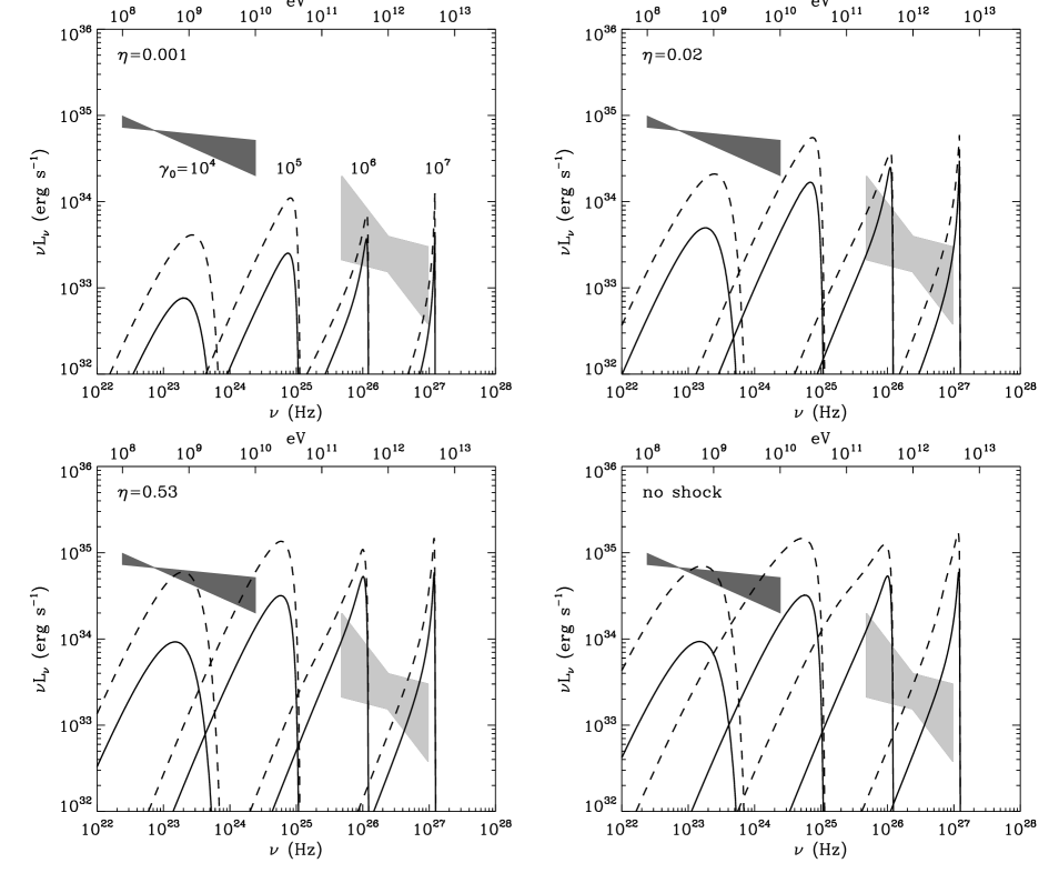
Figure 8: Spectral signature from the unshocked pulsar wind expected in LSI +61$\degr$303 and dependence with $\gamma_{0}$ and $\eta$. Spectra are averaged between phase $0.4<\phi<0.7$ (solid line, at periastron $\phi\equiv 0.23$) and the complementary phases $\phi<0.4$ or $\phi>0.7$ (dashed line). Luminosities are compared with the EGRET (dark bowtie) and MAGIC (light bowtie) observations, adopting a distance of 2.3 kpc. In the top left panel, $\eta=10^{-3}$ the shock is closed and the unshocked pulsar wind is assumed spherical. For $\eta=2$ $10^{-2}$ (top right panel) and $\eta=0.53$ (bottom left panel) the shock is open with half-opening angles $\alpha\sim 2\degr$ and $\alpha\sim 60\degr$ respectively. The bottom right panel shows the extreme case with no termination shock.

4 Discussion

The proximity of the massive star in LS 5039 and LSI +61$\degr$303  provides an opportunity to directly probe the distribution of particles in the highly relativistic pulsar wind. The calculations show the inverse Compton emission from the unshocked wind should be a significant contributor to the observed spectrum. For a monoenergetic and isotropic pulsar wind the emission remains line-like, with some broadening due to cooling, as had been found previously for the Crab and PSR B1259-63 (Bogovalov & Aharonian 2000; Ball & Kirk 2000). However, here, such line emission can pretty much be excluded by the available very high energy observations of HESS or MAGIC, and (to a lesser extent) by the EGRET observations that show power-law spectra at lower flux levels.

4.1 Is the pulsar wind power overestimated?

Reducing the pulsar power (or, equivalently, increasing the distance to the object) would diminish the predicted unshocked wind emission relative to the observed emission. This is not viable as this would also reduce the level of the shocked pulsar wind emission. Similarly, the energy carried by the particles may represent only a small fraction of the wind energy. At distances of order of the pulsar light cylinder the energy is mostly electromagnetic. Evidence that this energy is converted to the kinetic energy of the particles comes from plerions, which probe distances of order 0.1 pc from the pulsar. It is therefore conceivable that this conversion is not complete at the distances under consideration here (0.01-0.1 AU). In this case the emission from the particle component would be reduced. However, the shocked emission would also be reduced as high $\sigma$ shocks divert little of the energy into the particles (Kennel & Coroniti 1984). Furthermore, the high energy particles would preferentially emit synchrotron rather than inverse Compton due to the higher magnetic field. Hence, this possibility also seems unlikely.

Alternatively, the unshocked wind emission could be weaker compared to the shocked wind emission if the termination shock was closer to the pulsar, i.e. if one had a low $\eta$. In LS 5039 the unshocked wind emission is strong even with $\eta=0.001$, which already implies a stronger stellar wind than optical observations seem to warrant. Furthermore, the value of the magnetic field would be high if the termination shock was close to the pulsar and this inhibits the formation of very high energy gamma-rays as the high energy electrons would then preferentially lose energy to synchrotron radiation (Dubus 2006b). Hence, it does not seem viable either to invoke a smaller zone for the free wind.

The conclusion is that the strong emission from the pulsar wind found in the previous section is robust against general changes in the parameters used. The following subsections examine how this emission can be made consistent with the observations.

4.2 Constrains on the pulsar wind Lorentz factor

The high level of unshocked emission is compatible with the observations only if it occurs around 10 GeV or above 10 TeV, i.e. outside of the ranges probed by EGRET and the current generation of Cherenkov telescopes. This poses stringent constraints on the energy of the particles in the pulsar wind. The Lorentz factor of the pulsar wind would be constrained to a few $10^{5}$ or to more than $10^{7}$. The 1-100 GeV energy range will be partly probed by GLAST and HESS-2, and CTA in the more distant future. For instance, unshocked wind emission in LS 5039 would appear in the GLAST data as a spectral hardening at the highest energies. Nevertheless, that the free wind is emitting in the least accessible spectral region may appear too fortuitous for comfort.

4.3 Anisotropic pulsar wind

The assumptions on the pulsar wind may be inaccurate. Pulsar winds are thought to be anisotropic (Begelman & Li 1992). Bogovalov & Khangoulyan (2002) interpreted the jet-torus structure revealed by X-ray Chandra observations of the Crab nebula, as a latitude dependence of the Lorentz factor $\gamma(\theta)=\gamma_{i}+\gamma_{m}\sin^{2}\theta$ where $\gamma_{i}$ is small (say $10^{4}$) and $\gamma_{m}$ is high (say $10^{6}$). This hypothesis was corroborated by computational calculations in Komissarov & Lyubarsky (2004) where the synchrotron jet-torus was obtained. Here, the pulsar orientation to the observer is fixed (unless it precesses) so that the initial Lorentz factor of the pulsar wind along the line of sight would remain the same along the orbit. However, assuming the particle flux in the pulsar wind remains isotropic, the unshocked wind emission will appear at a lower energy and at a lower flux if the pulsar is seen more pole-on. The peak energy of the line-like spectral feature directly depends on $\gamma(\theta)$. Its intensity will also decrease in proportion as the pulsar power matches the latitude change in $\gamma$ to keep the particle flux isotropic (see Eq. 6).

The shocked wind emission is set by the mean power and Lorentz factor of the wind and is insensitive to orientation. However, a more pole-on orientation will lower the contribution from the unshocked component. For instance, if $\gamma(\theta)=10^{4}+10^{6}\sin^{2}\theta$ and $\theta=17\aas@@fstack{\circ}5$ then the effective $\gamma$ along the line-of-sight will be $10^{5}$ and the observed luminosity of the unshocked emission will be lowered by a factor 10 compared to the mean pulsar power (Eq. 6). The probability to have an orientation corresponding to a value of $\gamma(\theta)$ of 0.1 $\gamma_{m}$ or less is about ${\textstyle{1\over 5}}$, assuming a uniform distribution of orientations. This would be enough to push the line emission to lower energies and to lower fluxes by a factor 10 or more, thereby relaxing the constraints on the mean Lorentz factor of the wind. Although this is not improbable, it would again require some fortuitous coincidence for the pulsars in both LS 5039 and LSI +61$\degr$303 to be seen close enough to the pole that their free wind emission is not detected.

4.4 The energy distribution of the pairs

The assumption of a monoenergetic wind may be incorrect, if only because the particles in the pulsar wind are bathed by a strong external photon field even as they accelerate and that this may lead to a significantly different distribution. Fig. 9 shows the emission from a pulsar wind where the particles have been assumed to have a power-law distribution with an index of -2 between $\gamma$ of $10^{3}$ and $10^{8}$. Obviously, a power-law distribution of pairs erases the line-like spectral feature. The emission properties are essentially identical to the emission from the shocked region with a harder and fainter intrinsic Compton spectrum when the pulsar is seen in front of the star compared to when it is behind. The emission from the shocked region is also shown, calculated as in Dubus et al. (2008). The particle injection spectrum is the same in both regions. The particles are assumed to stay close to the pulsar and to escape from the shocked region after a time $t_{\rm esc}=R_{s}/(c/3)$ (top) and $10R_{s}/(c/3)$ (bottom). Longer $t_{\rm esc}$ do not change the distribution any further. The longer escape timescale enables a harder particle distribution to emerge at high energies (where the radiative timescale is comparable to $R_{s}/c$, see Fig. 2 in Dubus 2006b). With $t_{\rm esc}=R_{s}/(c/3)$, the shocked spectra is very close to the unshocked spectra. Generally, calculations show the spectra from the shocked and unshocked regions may be indistiguishable when the injected particles are taken to be the same in both regions. The only possible difference is that the longer residence time of particles in the shocked region allows for harder spectra.

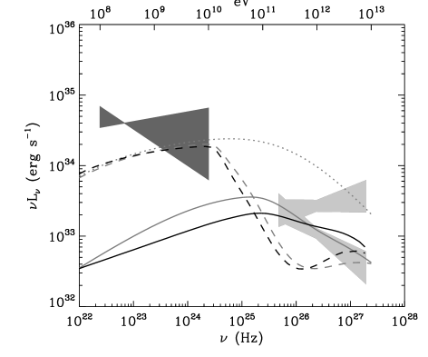
Figure 9: Comparison between emission from the shocked and unshocked regions in LS 5039, taking the same particle injection for both regions. The distribution is a power-law of index -2 between $\gamma=10^{3}$ and $10^{8}$ with total power $10^{36}$ erg s^-1. Spectra are averaged to correspond to the HESS ‘high state’ (solid lines) and ‘low state’ (dashed lines) as in Fig. 6. The geometry is a sphere of radius 2$\leavevmode\nobreak\ 10^{11}$ cm. Grey lines show emission from the unshocked emission and dark lines show the emission from the shocked region. The orbital averaged non-absorbed spectrum from the unshocked pulsar wind is shown in grey dotted line. Particles escape from the shocked region on a timescale $t_{\rm esc}=R_{s}/(c/3)$ (top) or $10R_{s}/(c/3)$ (bottom). The unshocked emission is the same in both panels.

4.5 Dominant emission from the unshocked wind

Emission from the unshocked wind could be the dominant contributor to the spectral energy distribution. In this case, the observations give the particle distribution in the pulsar wind. Sierpowska-Bartosik & Torres (2008) have considered such a scenario for LS 5039 and use a total energy in leptons of about $10^{35}$ erg s^-1 and a power-law distribution with an index around $-2$, both of which are adjusted to the observations and vary with orbital phase. The total pulsar power is much larger, 10³⁷ erg s^-1, in order to have a big enough free wind emission zone. Most of the pulsar energy is then carried by nuclei. Such a large luminosity would make the pulsar very young, comparable to the Crab pulsar, implying a high birth rate for such systems. Fig. 10 shows the expected emission from a pulsar wind propagating to infinity and with a particle power law index of -1.5 from $\gamma=10^{3}$ to $10^{8}$ chosen to adjust the ‘high state’ of LS 5039. The injected power is 4 10³⁵ erg s^-1. The injected spectrum gives a good fit of the ‘hard’ state. However, the ‘low’ state dominates the complete very high energy contribution ($\ga$ 1 TeV) due to the extended emitting region. Particles have enough time to radiate very high energy gammay-ray far away, where they are less affected by $\gamma-\gamma$ absorption.

A possible drawback of this scenario is that the synchrotron and inverse Compton emission are not tied by the shock conditions and that the total energy in leptons is low so that it is not clear how the radio, X-ray and gamma-ray observations below a few GeV would arise. It is also unclear how this can lead to a collimated radio outflow as seen in LSI +61$\degr$303. A possibility is emission from secondary pairs created in the stellar wind by cascading as suggested by Bosch-Ramon et al. (2008). More work is necessary to understand these different contributions and the signatures that may enable to distinguish them.

Another potential drawback of this scenario is that it does not explain why the very high energy gamma-ray flux is observed to peak close to apastron in LSI +61$\degr$303. If the inverse Compton scattering in the pulsar wind is responsible then the maximum should be around periastron, especially as gamma-gamma attenuation is very limited in LSI +61$\degr$303. On the other hand, if the emission arises from the shocked pulsar wind then synchrotron losses explain the lack of very high energy gamma-rays at periastron: the pulsar probes the dense equatorial wind from the Be star and the shock forms at a small distance, leading to a high magnetic field and a cutoff in the high-energy spectrum (see §6.2.2 in Dubus 2006b).

Figure 10: Fit to the observations of LS 5039, assuming the dominant contribution comes from the unshocked region of the pulsar wind. The ‘high state’ of HESS corresponds to the solid line, the ‘low state’ to the dashed line and the dotted line to the orbital averaged non-absorbed spectrum. The injected particles had a power law distribution with an index of $-1.5$ between $\gamma=10^{3}$ and 10⁸. The injected power is 4 $10^{35}$ erg s^-1.

5 Conclusion

Gamma-ray binaries are of particular interest in the study of pulsar wind nebula at very small scales. The massive star radiates a large amount of soft seeds photons for inverse Compton scattering on relativistic electrons from the pulsar. One expects two contributions in the gamma-ray spectral energy distribution: one from the shocked pulsar wind and another from the unshocked pulsar wind. The spectral signature from the unshocked region is strong and depends on the shock geometry and the initial energy of the pairs in the pulsar wind. A significant fraction of the pulsar wind power can be lost to inverse Compton scattering before a shock forms with the stellar wind (Sierpowska & Bednarek 2005). The shock location will thus be slightly closer in to the neutron star than calculated without taking into account the losses in the pulsar wind, assuming the wind is composed only of e⁺e^- pairs.

Significant emission from the free pulsar wind seems unavoidable. Inverse Compton losses in the free wind may be reduced if the shock occurs very close to the neutron star. This is unlikely as it would require a very strong stellar wind or a pulsar wind power that would be too low to produce the observed emission. If the pulsar wind is anisotropic then the orientation of the pulsar with respect to the observer can make the unshocked emission less conspicuous. This comes at the price of a peculiar orientation. If the pulsar wind is monoenergetic, then the line-like expected spectrum exceeds the observed very high energy power-laws for all geometries unless the pair energy is around 10 GeV or above 10 TeV. This pushes the direct emission from the wind in ranges where it may be constrained by future GLAST, HESS-2 or CTA measurements. The absence of any line emission will show that the assumption of a Crab-like monoenergetic, low $\sigma$ pulsar wind was simplistic. If the pairs in the pulsar wind have a power-law distribution, then the unshocked emission is essentially indistinguishable from the shocked emission (Sierpowska-Bartosik & Torres 2008). A promising alternative is the striped wind model in which the wind remains highly magnetised up to the termination shock, where the alternating field could be dissipated and accelerate particles (see Kirk et al. 2007 and references therein). Future theoretical studies on the generation of pulsar relativistic winds in the context of a strong source of photons may be able to yield the particle distribution to expect and lead to more accurate predictions.