Reflexion and Diffraction of Internal Waves analyzed with the Hilbert Transform

Abstract

We apply the Hilbert transform to the physics of internal waves in two-dimensional fluids. Using this demodulation technique, we can discriminate internal waves propagating in different directions: this is very helpful in answering several fundamental questions in the context of internal waves. We focus more precisely in this paper on phenomena associated with dissipation, diffraction and reflection of internal waves.

Keywords: Stratified fluids – Internal waves – Nonlinear Physics – Hilbert transform. PACS numbers: 47.55.Hd Stratified flows. 47.35.+i Hydrodynamic waves.

I Introduction

The Synthetic Schlieren technique [1] is a very powerful method to get precise and quantitative measurements for two-dimensional internal waves in stratified fluids. Such a technique was very effectively used to get quantitative insights while studying different mechanisms for internal waves. Let us just mention the emission, propagation and reflection of internal waves [2, 3, 4, 6, 5], or the generation and reflection of internal tides [6, 7, 8]. However, when considering internal waves generated by an oscillating body or by an oscillating flow over a topography, the analysis is drastically complicated by the possibility of different directions of propagation associated to a single frequency; such a problem arises also when multiple reflections occur at boundaries.

We present in this article a method to discriminate the different possible internal waves associated with one given frequency $\omega$. These waves can be discriminated by their wave vectors $\mathbf{k}=(k_{x},k_{z})$, according to the sign of both components, $k_{x}$ and $k_{z}$. The transformation we present here not only offers an analytical representation of the wave field which allows us to extract the envelope and the phase of the waves, but allows also to isolate a single wave beam. This method is based on the Hilbert transform (HT) previously applied to problems dealing with propagating waves, but adapted here to two-dimensional phenomena.

The method is used here to tackle several fundamental issues in order to bring new insights. It is important to emphasize that we used a source of monochromatic internal plane waves to facilitate the comparison with theoretical results.

The paper is organized as follows. In section II, we present the Hilbert transform. In the section II.4, we present its application to the classical oscillating cylinder experiment, with a special emphasis on the insights provided by the Hilbert Transform. In section III, we study three different physical situations that can be nicely solved with this technique. The dissipation length is studied in Sec. III.1, the back reflection on a slope in Sec. III.2, while Sec. III.3 focus on the diffraction mechanism. Finally section IV concludes the paper.

II Principle of the Hilbert Transform

II.1 Presentation of the variables

Before explaining on a simple example the different steps necessary to apply the Hilbert transform, let us briefly recall different properties of internal gravity waves. We consider a two-dimensional $(x,z)$ experimental situation and denote $t$ the time variable, $g$ the gravity and $\rho(x,z)$ the density. In a linearly stratified fluid such that ${\partial\rho}/{\partial z}<0$, and within the linear approximation, it is well-known [9] that the same wave equation

$$\triangle\psi_{tt}+N^{2}\psi_{xx}=0$$ (1)

is valid for the field $\psi(x,z,t)$ which stands for either the streamfunction, both velocity components, the pressure, or the density gradients. The constant

$$N=\sqrt{-\frac{g}{\rho}\frac{\partial\rho}{\partial z}}$$ (2)

which characterizes the oscillation of a fluid particle within a linearly stratified fluid is the so-called Brunt-Väisälä frequency. Looking for propagating plane waves solutions

$$\psi=\psi_{0}\,e^{i(\omega t-\mathbf{k.x})}\,,$$ (3)

where $\mathbf{x}=(x,z)$ and $\mathbf{k}=(k_{x},k_{z})$, one gets the dispersion relation

$$\omega^{2}=N^{2}\frac{k_{x}^{2}}{k_{x}^{2}+k_{z}^{2}}=N^{2}\sin^{2}\theta\,,$$ (4)

if one introduces $\theta$ the angle between the wavevector and the gravity. In this unusual dispersion relation, it is apparent that changing the sign of the frequency $\omega$ or the sign of any component $k_{x},k_{z}$ of the wavevector has no consequences. So four possible wavevectors are allowed for any given positive frequency, smaller than the Brunt-Väisälä frequency.

The Synthetic Schlieren technique gives quantitative measurements of the respectively horizontal and vertical density gradients, $\rho_{x}(x,z,t)$ and $\rho_{z}(x,z,t)$. As anticipated, both quantities verify Eq. (1). In the remainder of this section, we work on a field $U(x,z,t)$, which might be either $\rho_{x}(x,z,t)$, $\rho_{z}(x,z,t)$, or a velocity component as obtained in PIV experiments.

II.2 A simple one-dimensional example

We present here, in the first stage, how to compute the complex-valued field $\tilde{U}(x,z,t)$ such that $U(x,z,t)$ will correspond to its real part $Re(\tilde{U}(x,z,t))$. In order to do so, we demodulate the signal by applying the Hilbert transform. To avoid misunderstandings, let’s note that the Hilbert transform is sometimes the name of the operation that associates the real-valued field $Im(\tilde{U})$ to the real-valued field $U$, such that the complex number $\tilde{U}$ can be fully reconstructed. In this article, we call Hilbert transform (or complex demodulation) the operation associating the complex-valued field $\tilde{U}$ to the real field $U$. This demodulation technique has been previously used to compute local and instantaneous amplitudes, frequencies and wavenumbers [10, 11, 12] but, to the best of our knowledge, the present study is the first application in the context of internal gravity waves.

As an introductory example, let us consider a simple signal in one spatial dimension constructed as the superposition of two wave beams propagating in the vertical direction $z$ with the same frequency and the same wavenumber $k_{z}$

$$U(z,t)=A\cos(\omega t-k_{z}z)+B\cos(\omega t+k_{z}z).$$ (5)

As $z$ is the vertical component, the first term corresponds to a wave propagating upward, whereas the second one to a wave propagating downward. For the sake of simplicity, we further suppose that the amplitude $A$ and $B$ are constant in space and time. Rewriting the cosines as the sum of exponentials with complex arguments, and decomposing according to a Fourier transform in time, we have

$$U(z,t)=\hat{U}_{1}\,e^{i\omega t}+\hat{U}_{2}\,e^{-i\omega t}$$ (6)

where $\hat{U}_{1}=(Ae^{-ik_{z}z}+Be^{ik_{z}z})/2$ and $\hat{U}_{2}$ is the complex conjugate of $\hat{U}_{1}$. So if we filter out the negative frequencies in Fourier space, and multiply by a constant factor 2, we are left with

$$\tilde{U}(z,t)=A\,e^{i(\omega t-k_{z}z)}+B\,e^{i(\omega t+k_{z}z)}.$$ (7)

The real-valued signal $U(z,t)$ has been transformed into the complex-valued signal $\tilde{U}(z,t)$ such that $U(z,t)=Re(\tilde{U}(z,t))$. With that complex signal at hands, it is now easy to separate the two wave beams by looking at the Fourier transform in space

$$\tilde{U}(z,t)=(Ae^{i\omega t})\,e^{-ik_{z}z}+(Be^{i\omega t})\,e^{ik_{z}z}.$$ (8)

Isolating the positive (resp. negative) values of the wavenumber $k_{z}$ will isolate the wave propagating towards positive (resp. negative) $z$. It is important to stress that this second stage is only possible because $\tilde{U}$ is a complex valued signal and not a real valued one: its Fourier transform is therefore not the sum of two complex conjugated parts on positive and negative frequencies.

II.3 The two-steps procedure for two-dimensional waves

Let us now precise how we operate on real experimental data involving two spatial dimensions.

The first step, called demodulation, is obtained by performing sequentially the three following operations:

• a Fourier transform in time of the field $U(x,z,t)$,

• a wide or selective band-pass filtering in Fourier space around the positive fundamental angular frequency $\omega=2\pi f$, where we have introduced $f$ the temporal frequency measured in hertz.

• the inverse Fourier transform generating the complex signal $\tilde{U}(x,z,t)$.

On step ii) which removes exactly half the energy of the signal, we also perform a multiplication by a factor 2, to preserve the amplitude of the signal and to have $U=Re(\tilde{U})$.

It is crucial to realize that four different travelling waves are mixed in this complex signal

$$\tilde{U}(x,z,t)=\tilde{A}(x,z,t)+\tilde{B}(x,z,t)+\tilde{C}(x,z,t)+\tilde{D}(x,z,t)$$ (9)

with

$$\tilde{A}(x,z,t) = A(x,z,t)\,\exp{i(\omega t-k_{x}x-k_{z}z)}\,,$$ (10)

$$\tilde{B}(x,z,t) = B(x,z,t)\,\exp{i(\omega t-k_{x}x+k_{z}z)}\,,$$ (11)

$$\tilde{C}(x,z,t) = C(x,z,t)\,\exp{i(\omega t+k_{x}x-k_{z}z)}\,,$$ (12)

$$\tilde{D}(x,z,t) = D(x,z,t)\,\exp{i(\omega t+k_{x}x+k_{z}z)}\,.$$ (13)

Note that in Eqs (10)-(13), we have considered the wavenumbers $k_{x}$ and $k_{z}$ positive in order to identify more easily the direction of propagation.

Although the four waves oscillate in time at the same frequency $\omega$, they do not propagate in the same direction, because of the different signs in front of the wavenumbers $k_{x}$ and $k_{z}$ (cf. Fig. 1). Note that amplitudes $A$, $B$, $C$ and $D$ might depend on space and time: dissipation is a good example. However, scales on which they vary must be much larger than scales $\omega^{-1}$, $k_{x}^{-1}$ and $k_{z}^{-1}$ around which the demodulation is performed.

In the second step, we isolate the four waves $A$, $B$, $C$ and $D$, one from each other, using the complex-valued field $\tilde{U}(x,z,t)$. To do so, we apply another filtering operation in Fourier space, but this time in the wavenumber directions $k_{x}$ and $k_{z}$ associated with spatial directions $x$ and $z$. Again, this filtering is only possible on a complex field, i.e. after the Hilbert transform has been performed. The goal of this additional filtering is only to select positive or negative wavenumbers, but one might also take advantage to apply a more selective filter to remove spurious details and noise at other wavenumbers.

The two steps we have detailed involved successively a Fourier transform in time, and then in space directions. Of course, it is equivalent to operate first in a space direction and then in time and in the other space direction. The best choice is in fact imposed by the Fourier transforms resolution, i.e. the first Fourier transform has to be performed in the direction with the largest number of experimental points.

Figure 1: These pictures emphasize the four different travelling waves which might propagate in a stratified fluid. Left panel corresponds to the wavenumbers in the Fourier space while the right panel is in the direct space. Left panel defines the four different domains $A$, $B$, $C$ and $D$ corresponding to different signs of the wavenumber in the $x$ and $z$ space directions. Right panel presents also a synthetic view of the four internal wave beams emitted, in a 2D stratified fluid, by a vertically oscillating body located at the origin. For each beam, the phase velocity $\mathbf{c}_{\varphi}$ is parallel to the wavevector $\mathbf{k}$, but orthogonal to its associated group velocity $\mathbf{c}_{g}$. Note that, for example, the beam propagating in the bottom-right domain of the right panel, corresponds to a wavevector with both positive components, explaining that this domains is labelled $A$, according to (10).

According to the schematic figure 1, we then get a single wave corresponding to a specific direction of the wavevector where $A(x,z,t)$ is the complex-valued amplitude of the wave travelling to the right in the $x$-direction and travelling up in the $z$-direction. $B$, $C$ and $D$ are the complex-valued amplitudes of the three other possible waves. In the experiments, one has to measure first the frequency $\omega$ and the wavenumbers $k_{x}$, $k_{z}$, but we note that they are the same over all spatiotemporal data corresponding to a given experiment. The envelopes $A$, $B$, $C$ and $D$ contain information not carried by the fast frequencies $\omega$ and fast wavenumbers $k_{x},k_{z}$, such as amplitude envelopes of the beams, and local wavenumber modulations: we will study carefully these quantities.

In summary, the demodulation technique extracts from the experimental signal the complex quantity

$$\chi(x,z,t)=|\chi(X,Z,T)|\exp[i\varphi_{\chi}(x,z,t)]\,,$$ (14)

where $\chi$ stands for $A$, $B$, $C$ or $D$. The argument of the exponential, $\varphi_{\chi}$, is the fast-varying phase corresponding to wave $\chi$, rotating at the experimental signal frequency, while containing slow modulations.

In practice, the complex demodulation of the initial spatio-temporal signal $U(x,z,t)$ results in four sets of four fields (local and instantaneous):

• the amplitude $|\chi(x,z,t)|$,

• the frequency $\omega(x,z,t)=\partial\varphi_{\chi}/\partial t$,

• the wavenumber in the $x$-direction $k_{x}(x,z,t)=\partial\varphi_{\chi}/\partial x$,

• the wavenumber in the $z$-direction $k_{z}(x,z,t)=\partial\varphi_{\chi}/\partial z$.

Note that the wavenumbers and the frequency have to be calculated from the phase field.

Let us emphasize finally that, the Fourier transform being bijective only when applied to infinite or periodical signals, it is important to filter the data first in time, in order to benefit from the sharpness of time spectra obtained after long-time data acquisitions; in a second step, the Fourier transform in space is applied, allowing to separate waves $A$, $B$, $C$ or $D$.

The application of the Hilbert Transform (HT) to the study of internal waves can provide very interesting results and answer questions that remained unsolved. The main idea is to isolate the differences between internal wave beams propagating up or down, to the left or to the right. However, before considering such situations, we study in the following subsection how this method might be applied to a simple two-dimensional situation which has been intensively studied already.

II.4 The classical oscillating cylinder experiment as a first example

The first example one might consider is the simple experiment of a cylinder oscillating up and down at a given frequency $\omega$. Initiated by the Görtler experiment [13], this setup was later popularized by Mowbray and Rarity [14] and recently generalized to a three dimensional situation [15].

The experiment we will describe was realized in a tank of $120\,\textrm{x}\,50\,\textrm{x}\,10\,\textrm{cm}^{3}$ filled with linearly stratified salt water. Quantitative internal waves visualization were obtained by Synthetic Schlieren [1], which measures the horizontal and vertical density gradient perturbations referred as $\rho_{x}(x,z,t)$ and $\rho_{z}(x,z,t)$ in the following. If one considers an oscillating cylinder in a two-dimensional stratified fluid, the four internal wave beams emitted have four wavevectors differing one from each other by the sign of their projections onto $(Ox)$ and $(Oz)$, as summarized in Fig. 1(b).

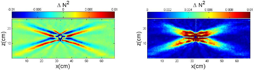
Figure 2: Saint Andrew’s cross obtained with a cylinder of radius $R=1.5\,$cm oscillating vertically with an amplitude $1.5\,$mm at a frequency $\omega=0.28\,\textrm{rad.s}^{-1}$ in a stratified fluid with Brunt-Väisälä frequency $N=1.0\,\textrm{rad.s}^{-1}$. The picture presents the real part (left panel) and amplitude (right panel) of the Hilbert transform, corresponding to the experimental horizontal density gradient $\rho_{x}$ filtered in time.

The complex demodulation of the wave field, in time first, is presented in Fig. 2. Such a picture clearly emphasizes that four different beams are generated by the oscillating cylinder, all of them being tilted with an angle $\theta$ with respect to the gravity, $\theta$ being given by the dispersion relation (4).

After an additional filtering along the $z$-coordinate, first, and then along the $x$-coordinate, four different beams can be isolated as presented in Fig. 3. Although some boundary effects can be detected at locations corresponding to discontinuities in space due to the cylinder, explaining the intense yellow areas along the horizontal and vertical axes, it is important to stress that there is no ambiguity concerning the field treated. Moreover, these side-effects might be corrected by applying the HT in space only to a selected domain instead of considering the full window of observation containing also the cylinder here.

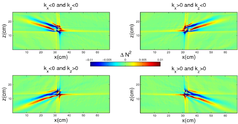
Figure 3: Real part of the horizontal density gradient $\rho_{x}$ presented in Fig. 2 after spatial filtering. The four different pictures correspond to the four possible waves described in Fig. 1(a).

We will now present two interesting points that have not been addressed in the previous literature (for recent results see [6, 20]) while studying the wavefield emitted by an oscillating cylinder.

Figure 4(a) presents a zoom on the phase of the beams emitted to the right of the cylinder (right side of Fig. 2): it is clear that there is no direct link between the phase evolution of the downward and upward propagating waves. Such an image will be very helpful when we will analyze the spatial structure of the emitted phase for the diffraction phenomenon in section III.3.

Figure 4(b) shows the evolution of the transverse spatial spectrum of the downward propagating wave to the right. They have been obtained by extracting the transverse profiles (along $(O\eta)$) at the circles located on the axis of propagation of the wave $(O\xi)$ and shown in Fig. 4(a). This picture reveals not only the decrease of the amplitude due to dissipation (see Sec. III.1 for a complete analysis) but also the gradual shift toward smaller value of the wavenumbers, i.e. toward larger wavelengths. [22]

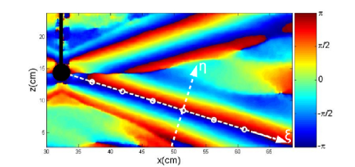
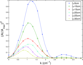
Figure 4: (Left panel) Phase of the density gradient $\rho_{x}(x,z,t)$ after step 1, zoomed on the right-hand side of Fig. 2. The cylinder is represented in black. Note also the definition of the variables $\xi$ and $\eta$, respectively along and transversal to the propagation. (Right panel) Evolution of the transverse spatial spectrum along the axis of propagation $(O\xi)$. Amplitudes have been normalized by the maximum value of the spectrum closest to the cylinder at $\xi=5$ cm.

In summary, the use of the Hilbert transform allows one to separate rather easily all the waves emitted from the cylinder, and to have a very precise definition of the phase of the wavefield, a quantity of importance to describe the wave spectra. We use in the next section these properties to address questions still pending.

III Applications

In the remainder of the article, we study internal waves beam emanating from a “pocket size” version [24] of the internal plane wave generator that we have recently developed [16]. All experiments were realized in a tank of $80\times 42.5\times 17\,\textrm{cm}^{3}$ filled with linearly stratified salt water. Horizontally oscillating plates of thickness $6\,\textrm{mm}$ create a sinusoïdal envelope of amplitude $a_{0}=5\,\textrm{mm}$ and wavelength $\lambda_{e}=3.9\,\textrm{cm}$, ($k_{e}=2\pi/\lambda_{e}$). The oscillating frequency $\omega$ defines through the dispersion relation (4) the angle of propagation of the beam with respect to the gravity. Such a device was shown to be extremely effective to generate nice plane wave beams in linearly stratified fluids [16].

III.1 Dissipation of internal waves

The first physical situation we consider is the dissipation of internal waves within a laboratory tank. The linear viscous theory developed by Thomas & Stevenson [17] first, and Hurley & Keady [18] afterwards, has been tested with good accuracy [2, 19, 20]. The damping of the averaged spectrum with time has also been studied, typically in the case of attractors because a steady state is obtained due to a balance between amplification at reflection and viscous damping [21, 22]. In Fig. 4(b), the damping of the spectrum along the axis of propagation can also be analyzed similarly. Nevertheless, these approaches are integral ones over all wavenumbers, and the viscous damping has not been tested on a monochromatic internal wave. The Hilbert Transform is moreover an excellent tool to measure the dissipation effects.

The structure expected [23] for a viscous internal plane wave is

$$\psi(\xi,\eta,t)=\psi_{0}\,e^{-\beta\,\xi}\,e^{i(\omega t-k\eta)}\,,$$ (15)

where $\xi$ is the longitudinal coordinate while $\eta$ corresponds to the transversal one. The quantity

$$\beta=\frac{\nu k^{3}}{2N\cos\theta}=\frac{\nu k^{3}}{2N\sqrt{1-\frac{\omega^{2}}{N^{2}}}}\,.$$ (16)

corresponds to the inverse dissipation length. Thanks to the analytical representation of the internal waves using the HT, it is easy to get the envelope of a monochromatic internal wave and thus quantify how it decreases through viscous dissipation. Results shown below correspond to three different stratifications.

For each frequency, the envelope of the emitted beam is extracted: a typical result is shown in Fig. 5(a). The logarithm along the $\xi$-coordinate is then plotted versus the longitudinal coordinate $\xi$ for different $\eta$-values, as illustrated in Fig. 5(b). The dissipation rate according to the direction of propagation is then obtained by the averaged linear fit over the different profiles extracted.

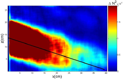
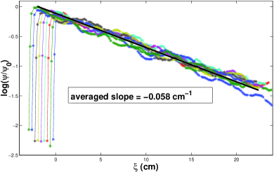
Figure 5: (a) Envelope of the Hilbert transform of the downward field $\rho_{x}(x,z,t)$ ($A$ and $C$) for an oscillating frequency $f=0.033\,$Hz and a Brunt-Väisälä frequency $N=0.66\,\textrm{rad.s}^{-1}$. The tilted black line indicates the location of one of the regularly extracted profiles. All other ones are parallel to this one. Panel (b) presents the logarithm of extracted profiles together with the averaged linear fit.

Repeating the above procedure for several frequencies, one gets the evolution of the dissipation length $\beta(\omega)$. It is however important to realize that, the propagation being tilted with respect to the vertical plane of emission, the forcing of the internal plane wave generator does not create a wave whose wavelength is $\lambda_{e}$. A projection of the wavelength on the direction perpendicular of propagation has to be taken into account: the wavevector of the propagating internal wave is therefore $k=k_{e}/\cos\theta$, so that we have the following relation

$$\beta=\frac{\nu k_{e}^{3}}{2N\cos^{4}\theta},$$ (17)

which can be rewritten in the more convenient form

$$N\beta=\frac{\nu k_{e}^{3}}{2}\frac{1}{(1-x^{2})^{2}}$$ (18)

by introducing $x=\omega/N$. It is thus generic to plot the attenuation rate $\beta$ times the Brunt-Väisälä frequency $N$ as a function of the ratio $x=\omega/N$ for different values of $N$, as presented in Fig. 6. Using the value of the viscosity $\eta=1.05\,10^{-6}$ m².s^-1, only one free parameter is remaining, the wavevector $k_{e}=2\pi/\lambda_{e}$.

Above procedure leads to the following result, $\lambda_{e}=3.55$ cm (+0.20/-0.16) cm, in good agreement with the value obtained from the transverse beam structure [24]. Surprisingly these values are slightly different from the one imposed by the internal plane wave generator. Figure 6 which presents the best fit attests the good agreement with experimental results. The model seems particularly accurate for frequencies $\omega$ sufficiently small compared to the cut-off frequency $N$.

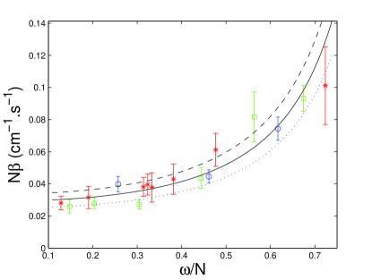
Figure 6: $N\beta$ as a function of $\omega/N$ for three different stratifications: stars, squares and circles correspond to experiment with $N=0.66$, 0.68 and 0.76 rad.s^-1. The solid curve corresponds to the best value for fitting the data, $\lambda_{e}=3.55$ cm, while the dashed (resp. dotted) line to the lower (resp. upper) bound $\lambda_{e}=3.39$ cm (resp. $\lambda_{e}=3.75$ cm).

III.2 Back-reflected waves on a slope.

We have also used the Hilbert Transform to identify a possible back-reflected wave when an incident internal wave beam is reflecting on a slope of angle $\alpha$ with the horizontal. After reflection, as shown by Fig. 7, two beams inclined with an angle $\theta$ with respect to the horizontal might be emitted from the slope. One of this beam has been experimentally reported several times [2, 4, 6, 5], contrary to the second one, aligned with the incident beam but propagating in the opposite direction and represented by the dashed arrow in Fig. 7. This additional beam was considered by Baines [25] and Sandstrom [27] when studying theoretically the effect of boundary curvature on reflection of internal waves. Let us experimentally prove that no back-reflection occurs at planar surfaces.

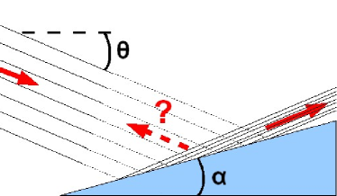
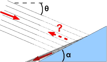
Figure 7: Left panel presents the principle of the possible back-reflection problem for an incident internal wave beam. Left panel shows the $\theta>\alpha$ case, while the right one presents the opposite case $\theta<\alpha$.

It is clear that if it exists the amplitude of the back-reflected beam has to be much smaller than the incident one, as usual techniques were unable either to identify it, or to exclude it. This is the reason why we have performed several experiments of an incident beam impinging onto a slope, away from critical incidence but also close to it (see Table 1 for values of control parameters). Analysis of one case with $\theta>\alpha$ is presented in Fig. 8. The back reflected beam in that case should be a $D$-wave according to classification (9). However, Fig. 8 shows absolutely no evidence of it, and only a $B$-component is visible. Nevertheless, as the HT along the $x$-coordinate has not been performed to avoid the introduction of spurious boundary effects, it is still possible to argue that the $D$-wave might be localized where the $B$-wave could shadow it. However, as this spatial domain remains extremely small, it is therefore very unlikely.

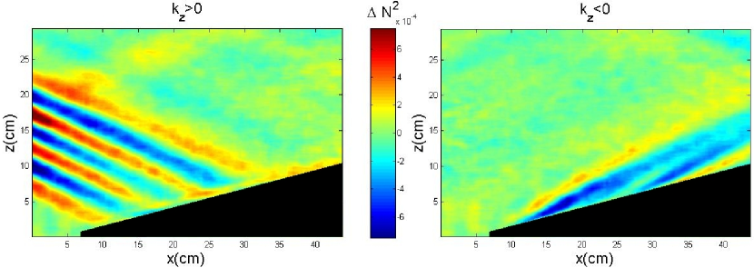
Figure 8: Horizontal density gradient $\rho_{x}$. (Left) Downward ($A$ and $C$) and (right) upward ($B$ and $D$) waves reflecting on a slope ($\alpha=14$), in $\Delta N^{2}$ rad².s^-2. The frequency of the waves was $\omega/N=0.43$ with the Brunt-Väisälä frequency $N=0.42~{}\textrm{rad.s}^{-1}$.

Run	1		2		3		4		5
$\theta$ (deg.)	14.	0	7.	0	11.	4	15.	1	25.	0
$\alpha$ (deg.)	25.	5	14.	5	14.	5	14.	5	14.	0
$\varepsilon$ (deg.)	-11.	5	-7.	5	-3.	1	0.	6	11.	0
$N$ (rad.s${}^{-1})$	0.	42	0.	58	0.	58	0.	58	0.	42

Table 1: Summary of experimental runs with all control parameters: $\theta$ the angle of energy propagation, $\alpha$ the angle of the slope, $\varepsilon=\theta-\alpha$ and $N$ the Brunt-Väisälä frequency.

Varying the angle $\theta$ of the waves around $\alpha$, the slope angle, no trace of back-reflected intensity are apparent, even close to critical conditions $\theta=\alpha$. In order to give a definitive answer, we have also considered the case $\theta<\alpha$ (see Fig. 7(b)). In that case, the back-reflected beam would be the only one to propagate upward, while the classically reflected beam would be a $C$-wave, propagating downward.

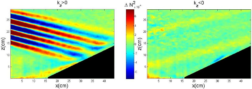
Figure 9: Horizontal density gradient $\rho_{x}$. (Left) Downward waves ($A$ and $C$) and (right) upward waves ($B$ and $D$) reflecting on a slope ($\alpha=25.5$), in $\Delta N^{2}$ rad².s^-2. The frequency of the waves was $\omega/N=0.24$ with the Brunt-Väisälä frequency $N=0.42~{}\textrm{rad.s}^{-1}$.

Figure 9 corresponding to such a case attests that there is no wave propagating backward. We can therefore claim that the back-reflected beam is definitely not present when internal waves reflect onto a slope. Concave or convex slopes might lead to different results [25].

III.3 Diffraction of internal waves

The diffraction of internal waves is the last issue we will consider in this paper. Although it is not directly interesting for oceanographic applications, it seems natural to ask [29] what is the equivalent of the Huygens-Fresnel principle for optical waves. Indeed, it has been established for centuries that when a plane wave encounters a thin slit, optical waves are reemitted in all directions. But what about internal waves? To the best of our knowledge, there is neither theoretical nor experimental results on this topic.

As the incident wave is impinging onto the slit with a well defined frequency, it is clear that the transmitted waves have to satisfy the dispersion relation (4). However, as schematically shown in Fig. 10(a), two different beams might be expected after the slit. In the case exemplified in this picture, it is clear that most of the energy will be transmitted to the waves propagating upward. Is it possible however to detect whether part of the energy is emitted downward? The main goal is therefore to be able to discriminate what is going out of a slit with a width comparable to the wavelength of an incoming internal plane wave.

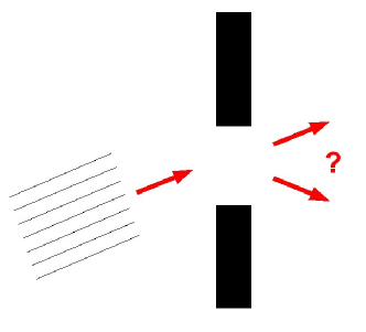
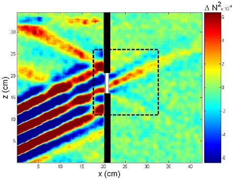
Figure 10: Left panel presents the principle of the diffraction problem for an incident internal wave beam. Right panel shows the horizontal density gradient $U$ field in $\Delta N^{2}$ rad².s^-2 for an incoming internal plane wave, corresponding to a wavelength $\lambda=3.6$ cm on a 4 cm wide slit. The dotted square corresponds to the region presented in Figs. 11 and 12.

In th experiments, the stratification is linear with $N=0.45~{}\textrm{rad.s}^{-1}$, while the incoming beam has a frequency $\omega=0.196~{}\textrm{rad.s}^{-1}$ and a wavelength $\lambda=3.2$ cm. Since the source is the internal plane wave generator, we remind that it corresponds to a vertical wavelength $\lambda_{z}=3.6$ cm. The slit of varying width $a$ is made of two sliding plastic plates of a thickness of $1$ cm, and is represented by a thick vertical white line in Figs. 10, 11 and 12, since no signal can be obtained in this region with the Synthetic Schlieren technique because of the sides of the slits. We present below results corresponding to widths of the slit $a=6$, 4, 3, and 2 cm. Note that for $a=1$ cm, no signal was obtained after the slit, which means that its intensity was below the noise level (if there was anything to measure).

Figures 11 and 12 present the results for $a=4$ cm and $a=2$ cm, emphasizing two different mechanisms for the emission that corresponds to $a>\lambda$ and $a<\lambda$. Note that both pictures present zooms close to the slit to better appreciate the interesting region.

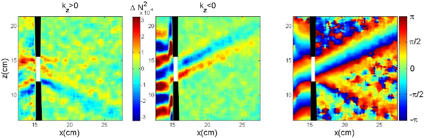
Figure 11: Large slit case. Hilbert transform of the gradient density field $\rho_{x}$ in $\Delta N^{2}$ $(\textrm{rad.s}^{-1})^{2}$ filtered at $\omega=0.196~{}\textrm{rad.s}^{-1}$ for $a=4$ cm with $k_{z}>0$ (left panel), $k_{z}<0$ (centered panel) and phase of the complete field with all values of $k_{z}$ (right panel).

In the first case, it is apparent that most of the intensity is in the beam emitted in the same direction than the incoming wave (upward propagation here). Furthermore, this beam seems very similar to the incoming plane wave: one notes indeed that the wavelength is identical before and after the slit. Moreover the continuity of the phase is nicely shown by the right panel of Fig. 11. Nevertheless, the edges of the slit are also a source emitting downward propagating beams since waves can be seen on both sides of the slit. It seems logical since the incoming plane wave creates an oscillating flow close to the slit, inducing a wavefield similar to the one of an oscillating body in a fluid at rest. It is finally important to notice that the spatial structure of the phase of the complete wave field is different from the one observed in Fig. 4 for an oscillating cylinder. The emission of the upward and downward propagating waves by the slit is consistent since there is no discontinuity in the spatial structure of the phase.

In the second case $a=2$ cm presented in Fig. 12 with a slit smaller than the wavelength, the mechanism is different. It seems that the only property similar to the incoming plane wave in the two beams transmitted through the slit is the frequency. Both transmitted beams have comparable intensities. The spatial structure of the phase presents a discontinuity strongly reminiscent of the wave field emitted by an oscillating body as shown by Fig. 4.

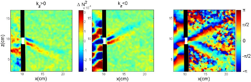
Figure 12: Small slit case. Hilbert transform of the horizontal density gradient field $\rho_{x}$ in $\Delta N^{2}$ $(\textrm{rad.s}^{-1})^{2}$ filtered at $\omega=0.196~{}\textrm{rad.s}^{-1}$ for $a=2$ cm with $k_{z}>0$ (left panel), $k_{z}<0$ (centered panel) and phase of the complete field with all values of $k_{z}$ (right panel).

To have a global view of the physics of internal plane waves diffraction, we finally present in Fig. 13 the vertical spatial spectra associated to the transmitted waves (upward and downward) taken at 1.5 cm after the slit for all values of the width $a$, in comparison with the spectrum of the incoming wave. The amplitudes of the Fourier components have been normalized by the maximum amplitude $|A_{incoming}|$ of the incoming wave spectrum measured $4$ cm before the slit. Several comments are in order. A clear shift of the peak toward larger values of the wavenumbers is visible when the width of the slit decreases. The spectra are also clearly enlarged. This is consistent with the previous remark that for a large slit the transmitted wave beam is very similar to the incident one. The spectra of the downward beam are visible in the negative $k$ half plane. In the large cases, $a=3$ and 4, they are wide and with a small amplitude attesting that most of the incident energy is transmitted upward, i.e. directly. On the contrary, in the thin slit case, $a=2$, the amplitudes for downward and upward propagating are comparable. It is difficult to propose a more quantitative discussion since the dissipation of the spectra is important.

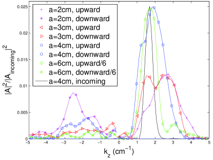
Figure 13: Spectra of the vertical cut of the horizontal density gradient $\rho_{x}$ measured $1.5$ cm on the right of the slit. The different curves corresponds to different widths $a$ of the slit (see inset for values).

In summary, the analysis of these spectra confirms that when the slit is sufficiently “large”, the emitted beam has a vertical wavenumber similar to the incoming one although the spectrum is slightly wider. On the contrary, when the slit is “small” enough, both beams have similar spectra and amplitudes.

Finally, we can conclude that the change in the type of waves emitted after the slit is due to the possibility of a spatial forcing of the phase by the incoming plane wave. The latter involves a typical length, the inverse of the vertical number $k_{z}$, which is in the present experiment nothing but the wavenumber forced by the generator. It appears that a criterion for a change in behavior occurs when the spatial evolution of the phase is small compared to the temporal one, leading to $k_{z}a\leq\omega T$, i.e. $k_{z}a\leq 2\pi$. In the present case, it leads to $a\leq\lambda_{e}=3.6$ cm. The main question remaining is to find a precise criterion to discriminate when spatial forcing of the phase occurs or not. This phenomenon of phase forcing might be related to circular oscillations of a cylinder in a stratified fluid which leads to two preferential emission (two beams instead of four). [30, 31]

IV Conclusion

In this article, we have applied the complex demodulation, also called Hilbert transform. This transformation is shown to be very powerful when adapted to internal waves in two dimensions. The experimental investigation of attenuation, reflection and diffraction of internal plane waves generated using a new type of generator has brought answers to several theoretical assumptions never confirmed.

The attenuation of internal plane waves is in good agreement with the linear viscous theory of internal waves. Furthermore, the results obtained quantify the influence of the wavelength since we consider monochromatic internal plane waves.

Although the reflection of internal waves is a classic phenomenon, some theoretical ideas remained assumptions, and by looking for an hypothetical back-reflected wave we can now confirm that the back-reflection is not present.

Finally, we study the problem of diffraction of internal waves as it has not been investigated to our knowledge yet, and we exhibit the diffraction pattern of internal wave which is atypical due to the peculiar dispersion relation of internal waves.

Acknowledgments

We thank Denis Le Tourneau and Marc Moulin for their helps in preparing the experimental facility. This work has been partially supported by the 2006 IDAO-CNRS, 2007 LEFE-CNRS program and by 2005-ANR project TOPOGI-3D.

References

- [1] S. B. Dalziel, G. O. Hughes, and B. R. Sutherland. Whole-field density measurements by ‘synthetic schlieren’. Experiments in Fluids, 28:322–335, 2000.
- [2] B. R. Sutherland, S. B. Dalziel, G. O. Hughes, and P. F. Linden. Visualization and measurement of internal waves by ’synthetic schlieren’. part 1. vertically oscillating cylinder. Journal of Fluid Mechanics, 390:93–126, 1999.
- [3] T. Peacock and P. Weidman The effect of rotation on conical internal wave beams. Expteriments in Fluids, 39:32 2005.
- [4] T. Peacock and A. Tabaei. Visualization of nonlinear effects in reflecting internal wave beams. Physics of Fluids 17:061702, 2005.
- [5] A. Nye and S. B. Dalziel. Scattering of internal gravity waves from rough topography. In Proceedings of the 6th International Symposium on Stratified Flows, Perth. Ed. G. Ivey. 631-636, 2006.
- [6] L. Gostiaux. Étude expérimentale des ondes de gravité internes en présence de topographie. Émission, propagation, réflexion. PhD thesis, ENS Lyon, 2006.
- [7] L. Gostiaux and T. Dauxois. Laboratory experiments on the generation of internal tidal beams over steep slopes. Physics of Fluids 19: 028102 (2007).
- [8] T. Peacock, P. Echeverri, and N. J. Balmforth. An experimental investigation of internal waves beam generation by two-dimensional topography. Journal of Physical Oceanography 38:235-242, 2008.
- [9] P. K. Kundu. Fluid Mechanics. Academic Press, 1990.
- [10] V. Croquette and H. Williams. Nonlinear waves of the oscillatory instability on finite convective rolls. Physica D, 37:300–314, 1989.
- [11] N. B. Garnier, A. Chiffaudel, F. Daviaud, and A. Prigent. Nonlinear dynamics of waves and modulated waves in 1d thermocapillary flows. i. general presentation and periodic solutions. Physica D, 174:1–29, 2003.
- [12] N. B. Garnier, A. Chiffaudel, and F. Daviaud. Nonlinear dynamics of waves and modulated waves in 1d thermocapillary flows. ii. convective/absolute transitions. Physica D, 174:30–55, 2003.
- [13] H. Görtler. Über eine schwingungserscheinung in flüssigkeiten mit stabiler dichteschichtung. Zeitschrift für Angewandte Mathematik und Mechanik, 23:65–71, 1943.
- [14] D. E. Mowbray and B. S. H. Rarity. A theoretical and experimental investigation of the phase configuration of internal waves of small amplitude in a density stratified fluid. Journal of Fluid Mechanics, 28:1–16, 1967.
- [15] K. Onu, M. R. Flynn, and B. R. Sutherland. Schlieren measurement of axisymmetric internal wave amplitudes. Experiments in Fluids, 35:24–31, 2003.
- [16] L. Gostiaux, H. Didelle, S. Mercier, and T. Dauxois. A novel internal waves generator. Experiments in Fluids, 42:123–130, 2007.
- [17] N. H. Thomas and T. N. Stevenson. A similarity solution for viscous internal waves. Journal of Fluid Mechanics, 54:495–506, 1972.
- [18] D. G. Hurley and G. Keady. The generation of internal waves by vibrating elliptic cylinders. part2. approximate viscous solution. Journal of Fluid Mechanics, 351:119–138, 1997.
- [19] B. R. Sutherland and P. F. Linden. Internal wave excitation by a vertically oscillating elliptical cylinder. Physics of Fluids, 14:721–731, 2002.
- [20] H. P. Zhang, B. King, and H. L. Swinney. Experimental study of internal gravity waves generated by supercritical topography. Physics of Fluids, 19:096602, 2007.
- [21] M. Rieutord, B. Georgeot, and L. Valdettaro. Inertial waves in a rotating spherical shell: Attractors and asymptotic spectrum. Journal of Fluid Mechanics, 435:103–144, 2001.
- [22] J. Hazewinkel, P. van Breevoort, S. B. Dalziel, and L. R.M. Maas. Observations on the wavenumber spectrum and evoution of an internal wave attractor. Journal of Fluid Mechanics, 598:373–382, 2008.
- [23] J. Lighthill. Waves in Fluids. Cambridge Mathematical Library, printing edition, 1978.
- [24] M. Mercier, L. Gostiaux, and T. Dauxois. Internal waves generator. In preparation, 2008.
- [25] P. G. Baines. The reflexion of internal/inertial waves from bumpy surfaces. Journal of Fluid Mechanics, 46:273–291, 1971.
- [26] P. G. Baines. The reflexion of internal/inertial waves from bumpy surfaces. part 2. split reflexion and diffraction. Journal of Fluid Mechanics, 49:113–131, 1971.
- [27] H. Sandstrom. The effect of boundary curvature on reflection of internal waves. Mémoires Société Royale des Sciences de Liège, 6ème série, tome IV, 183-190, 1972.
- [28] T. Dauxois and W. R. Young. Near-critical reflection of internal waves. Journal of Fluid Mechanics, 390:271–295, 1999.
- [29] L. Maas. Private communication, 2005.
- [30] N. V. Gavrilov, E. V. Ermanyuk. Internal waves generated by circular translational motion of a cylinder in a linearly straified fluid. Journal of Applied Mechanics and Technical Physics 38: 224–227, 1996.
- [31] D. G. Hurley, M. J. Hood. The generation of internal waves by vibrating elliptic cylinders. Part 3. Angular oscillations and comparison of theiry with recent experimental observations. Journal of Fluid Mechanics 433, 61–75, 2001.