Catching Up Faster by Switching Sooner:
A Prequential Solution to the AIC-BIC Dilemma

Abstract

Bayesian model averaging, model selection and its approximations such as BIC are generally statistically consistent, but sometimes achieve slower rates of convergence than other methods such as AIC and leave-one-out cross-validation. On the other hand, these other methods can be inconsistent. We identify the catch-up phenomenon as a novel explanation for the slow convergence of Bayesian methods. Based on this analysis we define the switch distribution, a modification of the Bayesian marginal distribution. We show that, under broad conditions, model selection and prediction based on the switch distribution is both consistent and achieves optimal convergence rates, thereby resolving the AIC-BIC dilemma. The method is practical; we give an efficient implementation. The switch distribution has a data compression interpretation, and can thus be viewed as a “prequential” or MDL method; yet it is different from the MDL methods that are usually considered in the literature. We compare the switch distribution to Bayes factor model selection and leave-one-out cross-validation.

1 Introduction: The Catch-Up Phenomenon

We consider inference based on a countable set of models (sets of probability distributions), focusing on two tasks: model selection and model averaging. In model selection tasks, the goal is to select the model that best explains the given data. In model averaging, the goal is to find the weighted combination of models that leads to the best prediction of future data from the same source.

An attractive property of some criteria for model selection is that they are consistent under weak conditions, i.e. if the true distribution $P^{*}$ is in one of the models, then the $P^{*}$-probability that this model is selected goes to one as the sample size increases. BIC [Schwarz, 1978], Bayes factor model selection [Kass and Raftery, 1995], Minimum Description Length (MDL) model selection [Barron et al., 1998] and prequential model validation [Dawid, 1984] are examples of widely used model selection criteria that are usually consistent. However, other model selection criteria such as AIC [Akaike, 1974] and leave-one-out cross-validation (LOO) [Stone, 1977], while often inconsistent, do typically yield better predictions. This is especially the case in nonparametric settings of the following type: $P^{*}$ can be arbitrarily well-approximated by a sequence of distributions in the (parametric) models under consideration, but is not itself contained in any of these. In many such cases, the predictive distribution converges to the true distribution at the optimal rate for AIC and LOO [Shibata, 1983, Li, 1987], whereas in general MDL, BIC, the Bayes factor method and prequential validation only achieve the optimal rate to within an $O(\log n)$ factor [Rissanen et al., 1992, Foster and George, 1994, Yang, 1999, Grünwald, 2007]. In this paper we reconcile these seemingly conflicting approaches [Yang, 2005a] by improving the rate of convergence achieved in Bayesian model selection without losing its consistency properties. First we provide an example to show why Bayes sometimes converges too slowly.

1.1 The Catch-Up Phenomenon

Given priors on parametric models $\mathcal{M}_{1}$, $\mathcal{M}_{2}$, $\ldots$ and parameters therein, Bayesian inference associates each model $\mathcal{M}_{k}$ with the marginal distribution $\bar{p}_{k}$, given by

$$\bar{p}_{k}(x^{n})=\int_{\theta\in\Theta_{k}}p_{\theta}(x^{n})w(\theta)\,\text{d}\theta.$$

obtained by averaging over the parameters according to the prior. In Bayes factor model selection the preferred model is the one with maximum a posteriori probability. By Bayes’ rule this is $\operatorname{arg\,max}_{k}\bar{p}_{k}(x^{n})w(k)$, where $w(k)$ denotes the prior probability of $\mathcal{M}_{k}$. We can further average over model indices, a process called Bayesian Model Averaging (BMA). The resulting distribution $p_{\text{\rm bma}}(x^{n})=\sum_{k}\bar{p}_{k}(x^{n})w(k)$ can be used for prediction. In a sequential setting, the probability of a data sequence $x^{n}:=x_{1},\ldots,x_{n}$ under a distribution $p$ typically decreases exponentially fast in $n$. It is therefore common to consider $-\log p(x^{n})$, which we call the code length of $x^{n}$ achieved by $p$. We take all logarithms to base $2$, allowing us to measure code length in bits. The name code length refers to the correspondence between code length functions and probability distributions based on the Kraft inequality, but one may also think of the code length as the accumulated log loss that is incurred if we sequentially predict the $x_{i}$ by conditioning on the past, i.e. using $p(\cdot|x^{i-1})$ [Barron et al., 1998, Grünwald, 2007, Dawid, 1984, Rissanen, 1984]. For BMA, we have

$$-\log p_{\text{\rm bma}}(x^{n})=-\log\prod_{i=1}^{n}p_{\text{\rm bma}}(x_{i}\mid x^{i-1})=\sum_{i=1}^{n}\left[-\log p_{\text{\rm bma}}(x_{i}\mid x^{i-1})\right].$$

Here the $i$th term represents the loss incurred when predicting $x_{i}$ given $x^{i-1}$ using $p_{\text{\rm bma}}(\cdot|x^{i-1})$, which turns out to be equal to the posterior average: $p_{\text{\rm bma}}(x_{i}|x^{i-1})=\sum_{k}\bar{p}_{k}(x_{i}|x^{i-1})w(k|x^{i-1})$.

Prediction using $p_{\text{\rm bma}}$ has the advantage that the code length it achieves on $x^{n}$ is close to the code length of $\bar{p}_{\hat{k}}$, where $\hat{k}$ is the best of the marginals $\bar{p}_{1},\bar{p}_{2},\ldots$, i.e. $\hat{k}$ achieves $\min_{k}-\log\bar{p}_{k}(x^{n})$. More precisely, given a prior $w$ on model indices, the difference between $-\log p_{\text{\rm bma}}(x^{n})=-\log(\sum_{k}\bar{p}_{k}(x^{n})w(k))$ and $-\log\bar{p}_{\hat{k}}(x^{n})$ must be in the range $[0,-\log w(\hat{k})]$, whatever data $x^{n}$ are observed. Thus, using BMA for prediction is sensible if we are satisfied with doing essentially as well as the best model under consideration. However, it is often possible to combine $\bar{p}_{1},\bar{p}_{2},\ldots$ into a distribution that achieves smaller code length than $\bar{p}_{\hat{k}}$! This is possible if the index $\hat{k}$ of the best distribution changes with the sample size in a predictable way. This is common in model selection, for example with nested models, say $\mathcal{M}_{1}\subset\mathcal{M}_{2}$. In this case $\bar{p}_{1}$ typically predicts better at small sample sizes (roughly, because $\mathcal{M}_{2}$ has more parameters that need to be learned than $\mathcal{M}_{1}$), while $\bar{p}_{2}$ predicts better eventually. Figure 1 illustrates this phenomenon.

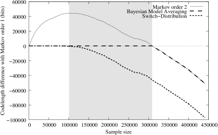
Figure 1: The Catch-up Phenomenon

It shows the accumulated code length difference $-\log\bar{p}_{2}(x^{n})-(-\log\bar{p}_{1}(x^{n}))$ on “The Picture of Dorian Gray” by Oscar Wilde, where $\bar{p}_{1}$ and $\bar{p}_{2}$ are the Bayesian marginal distributions for the first-order and second-order Markov chains, respectively, and each character in the book is an outcome. We used uniform (Dirichlet$(1,1,\ldots,1)$) priors on the model parameters (i.e., the “transition probabilities”) , but the same phenomenon occurs with other common priors , such as Jeffreys”. Clearly $\bar{p}_{1}$ is better for about the first $100\,000$ outcomes, gaining a head start of approximately $40\,000$ bits. Ideally we should predict the initial $100\,000$ outcomes using $\bar{p}_{1}$ and the rest using $\bar{p}_{2}$. However, $p_{\text{\rm bma}}$ only starts to behave like $\bar{p}_{2}$ when it catches up with $\bar{p}_{1}$ at a sample size of about $310\,000$, when the code length of $\bar{p}_{2}$ drops below that of $\bar{p}_{1}$. Thus, in the shaded area $p_{\text{\rm bma}}$ behaves like $\bar{p}_{1}$ while $\bar{p}_{2}$ is making better predictions of those outcomes: since at $n=100\,000$, $\bar{p}_{2}$ is $40\,000$ bits behind, and at $n=310\,000$, it has caught up, in between it must have outperformed $\bar{p}_{1}$ by $40\,000$ bits!

Note that the example models $\mathcal{M}_{1}$ and $\mathcal{M}_{2}$ are very crude; for this particular application much better models are available. Thus $\mathcal{M}_{1}$ and $\mathcal{M}_{2}$ serve as a simple illustration only (see the discussion in Section 8.1). However, our theorems, as well as experiments with nonparametric density estimation on which we will report elsewhere, indicate that the same phenomenon also occurs with more realistic models. In fact, the general pattern that first one model is better and then another occurs widely, both on real-world data and in theoretical settings. We argue that failure to take this effect into account leads to the suboptimal rate of convergence achieved by Bayes factor model selection and related methods. We have developed an alternative method to combine distributions $\bar{p}_{1}$ and $\bar{p}_{2}$ into a single distribution $p_{\text{\rm sw}}$, which we call the switch distribution, defined in Section 2. Figure 1 shows that $p_{\text{\rm sw}}$ behaves like $\bar{p}_{1}$ initially, but in contrast to $p_{\text{\rm bma}}$ it starts to mimic $\bar{p}_{2}$ almost immediately after $\bar{p}_{2}$ starts making better predictions; it essentially does this no matter what sequence $x^{n}$ is actually observed. $p_{\text{\rm sw}}$ differs from $p_{\text{\rm bma}}$ in that it is based on a prior distribution on sequences of models rather than simply a prior distribution on models. This allows us to avoid the implicit assumption that there is one model which is best at all sample sizes. After conditioning on past observations, the posterior we obtain gives a better indication of which model performs best at the current sample size, thereby achieving a faster rate of convergence. Indeed, the switch distribution is very closely related to earlier algorithms for tracking the best expert developed in the universal prediction literature; see also Section 7 [Herbster and Warmuth, 1998, Vovk, 1999, Volf and Willems, 1998, Monteleoni and Jaakkola, 2004]; however, the applications we have in mind and the theorems we prove are completely different.

1.2 Organization

The remainder of the paper is organized as follows (for the reader’s convenience, we have attached a table of contents at the end of the paper). In Section 2 we introduce our basic concepts and notation, and we then define the switch distribution. While in the example above, we switched between just two models, the general definition allows switching between elements of any finite or countably infinite set of models. In Section 3 we show that model selection based on the switch distribution is consistent (Theorem 1). Then in Section 4 we show that the switch distribution achieves a rate of convergence that is never significantly worse than that of Bayesian model averaging, and we show that, in contrast to Bayesian model averaging, the switch distribution achieves the worst-case optimal rate of convergence when it is applied to histogram density estimation. In Section 5 we develop a number of tools that can be used to bound the rate of convergence in Cesàro-mean in more general parametric and nonparametric settings, which include histogram density estimation as a special case. In Section 5.3 and Section 5.4 we apply these tools to show that the switch distribution achieves minimax convergence rates in density estimation based on exponential families and in some nonparametric linear regression problems. In Section 6 we give a practical algorithm that computes the switch distribution. Theorem 14 of that section shows that the run-time for $k$ predictors is $\Theta(n\cdot k)$ time. In Sections 7 and Section 8 we put our work in a broader context and explain how our results fit into the existing literature. Specifically, Section 7.1 explains how our result can be reconciled with a seemingly contradictory recent result of Yang [2005a], and Section 8.1 describes a strange implication of the catch-up phenomenon for Bayes factor model selection. The proofs of all theorems are in Appendix 0.A (except the central results of Section 5, which are proved in the main text).

2 The switch distribution for Model Selection and Prediction

2.1 Preliminaries

Suppose $X^{\infty}=(X_{1}$, $X_{2}$, $\ldots)$ is a sequence of random variables that take values in sample space $\mathcal{X}\subseteq\mathbb{R}^{d}$ for some $d\in\mathbb{Z}^{+}=\{1,2,\ldots\}$. For $n\in\mathbb{N}=\{0,1,2,\ldots\}$, let $x^{n}=(x_{1}$, $\ldots$, $x_{n})$ denote the first $n$ outcomes of $X^{\infty}$, such that $x^{n}$ takes values in the product space $\mathcal{X}^{n}=\mathcal{X}_{1}\times\cdots\times\mathcal{X}_{n}$. (We let $x^{0}$ denote the empty sequence.) For $m>n$, we write $X_{n+1}^{m}$ for $(X_{n+1}$, $\ldots$, $X_{m})$, where $m=\infty$ is allowed. We omit the subscript when $n=0$, writing $X^{m}$ rather than $X^{m}_{1}$.

Any distribution $P(X^{\infty})$ may be defined in terms of a sequential prediction strategy $p$ that predicts the next outcome at any time $n\in\mathbb{N}$. To be precise: Given the previous outcomes $x^{n}$ at time $n$, a prediction strategy should issue a conditional density $p(X_{n+1}|x^{n})$ with corresponding distribution $P(X_{n+1}|x^{n})$ for the next outcome $X_{n+1}$. Such sequential prediction strategies are sometimes called prequential forecasting systems [Dawid, 1984]. An instance is given in Example 1 below. Whenever the existence of a ‘true’ distribution $P^{*}$ is assumed — in other words, $X^{\infty}$ are distributed according $P^{*}$ —, we may think of any prediction strategy $p$ as a procedure for estimating $P^{*}$, and in such cases, we will often refer to $p$ an estimator. For simplicity, we assume throughout that the density $p(X_{n+1}|x^{n})$ is taken relative to either the usual Lebesgue measure (if $\mathcal{X}$ is continuous) or the counting measure (if $\mathcal{X}$ is countable). In the latter case $p(X_{n+1}|x^{n})$ is a probability mass function. It is natural to define the joint density $p(x^{m}|x^{n})=p(x_{n+1}|x^{n})\cdots p(x_{m}|x^{m-1})$ and let $P(X_{n+1}^{\infty}|x^{n})$ be the unique distribution on $\mathcal{X}^{\infty}$ such that, for all $m>n$, $p(X_{n+1}^{m}|x^{n})$ is the density of its marginal distribution for $X_{n+1}^{m}$. To ensure that $P(X_{n+1}^{\infty}|x^{n})$ is well-defined even if $\mathcal{X}$ is continuous, we will only allow prediction strategies satisfying the natural requirement that for any $k\in\mathbb{Z}^{+}$ and any fixed measurable event $A_{k+1}\subseteq\mathcal{X}_{k+1}$ the probability $P(A_{k+1}|x^{k})$ is a measurable function of $x^{k}$. This requirement holds automatically if $\mathcal{X}$ is countable.

2.2 Model Selection and Prediction

In model selection the goal is to choose an explanation for observed data $x^{n}$ from a potentially infinite list of candidate models $\mathcal{M}_{1}$, $\mathcal{M}_{2}$, $\ldots$ We consider parametric models, which we define as sets $\{p_{\theta}:\theta\in\Theta\}$ of prediction strategies $p_{\theta}$ that are indexed by elements of $\Theta\subseteq\mathbb{R}^{d}$, for some smallest possible $d\in\mathbb{N}$, the number of degrees of freedom. A model is more commonly viewed as a set of distributions, but since distributions can be viewed as prediction strategies as explained above, we may think of a model as a set of prediction strategies as well. Examples of model selection are histogram density estimation [Rissanen et al., 1992] ($d$ is the number of bins minus 1), regression based on a set of basis functions such as polynomials ($d$ is the number of coefficients of the polynomial), and the variable selection problem in regression [Shibata, 1983, Li, 1987, Yang, 1999] ($d$ is the number of variables). A model selection criterion is a function $\delta:\bigcup_{n=0}^{\infty}\mathcal{X}^{n}\rightarrow\mathbb{Z}^{+}$ that, given any data sequence $x^{n}\in\mathcal{X}^{n}$ of arbitrary length $n$, selects the model $\mathcal{M}_{k}$ with index $k=\delta(x^{n})$.

With each model $\mathcal{M}_{k}$ we associate a single prediction strategy $\bar{p}_{k}$. The bar emphasizes that $\bar{p}_{k}$ is a meta-strategy based on the prediction strategies in $\mathcal{M}_{k}$. In many approaches to model selection, for example AIC and LOO, $\bar{p}_{k}$ is defined using some parameter estimator $\hat{\theta}_{k}$, which maps a sequence $x^{n}$ of previous observations to an estimated parameter value that represents a “best guess” of the true/best distribution in the model. Prediction is then based on this estimator: $\bar{p}_{k}(X_{n+1}\mid x^{n})=p_{\hat{\theta}_{k}(x^{n})}(X_{n+1}\mid x^{n})$, which also defines a joint density $\bar{p}_{k}(x^{n})=\bar{p}_{k}(x_{1})\cdots\bar{p}_{k}(x_{n}|x^{n-1})$. The Bayesian approach to model selection or model averaging goes the other way around. It starts out with a prior $w$ on $\Theta_{k}$, and then defines the Bayesian marginal density

$$\bar{p}_{k}(x^{n})=\int_{\theta\in\Theta_{k}}p_{\theta}(x^{n})w(\theta)\,\text{d}\theta.$$ (1)

When $\bar{p}_{k}(x^{n})$ is non-zero this joint density induces a unique conditional density

$$\bar{p}_{k}(X_{n+1}\mid x^{n})=\frac{\bar{p}_{k}(X_{n+1},x^{n})}{\bar{p}_{k}(x^{n})},$$

which is equal to the mixture of $p_{\theta}$ according to the posterior, $w(\theta|x^{n})=p_{\theta}(x^{n})w(\theta)/\int p_{\theta}(x^{n})w(\theta)\,\text{d}\theta$, based on $x^{n}$. Thus the Bayesian approach also defines a prediction strategy $\bar{p}_{k}(X_{n+1}|x^{n})$.

Associating a prediction strategy $\bar{p}_{k}$ with each model $\mathcal{M}_{k}$ is known as the prequential approach to statistics [Dawid, 1984] or predictive MDL [Rissanen, 1984]. Regardless of whether $\bar{p}_{k}$ is based on parameter estimation or on Bayesian predictions, we may usually think of it as a universal code relative to $\mathcal{M}_{k}$ [Grünwald, 2007].

Example 1.

Suppose $\mathcal{X}=\{0,1\}$. Then a prediction strategy $\bar{p}$ may be based on the Bernoulli model $\mathcal{M}=\{p_{\theta}\mid\theta\in[0,1]\}$ that regards $X_{1},X_{2},\ldots$ as a sequence of independent, identically distributed Bernoulli random variables with $P_{\theta}(X_{n+1}=1)=\theta$. We may predict $X_{n+1}$ using the maximum likelihood (ML) estimator based on the past, i.e. using $\hat{\theta}(x^{n})=n^{-1}\sum_{i=1}^{n}x_{i}$. The prediction for $x_{1}$ is then undefined. If we use a smoothed ML estimator such as the Laplace estimator, $\hat{\theta}^{\prime}(x^{n})=(n+2)^{-1}(\sum_{i=1}^{n}x_{i}+1)$, then all predictions are well-defined. It is well-known that the predictor $\bar{p}^{\prime}$ defined by $\bar{p}^{\prime}(X_{n+1}\mid x^{n})=p_{\hat{\theta}^{\prime}(x^{n})}(X_{n+1})$ equals the Bayesian predictive distribution based on a uniform prior. Thus in this case a Bayesian predictor and an estimation-based predictor coincide!

In general, for a parametric model $\mathcal{M}_{k}$, we can define $\bar{p}_{k}(X_{n+1}\mid x^{n})=p_{{\hat{\theta}^{\prime}}_{k}(x^{n})}(X_{n+1})$ for some smoothed ML estimator $\hat{\theta}^{\prime}_{k}$. The joint distribution with density $\bar{p}_{k}(x^{n})$ will then resemble, but in general not be precisely equal to, the Bayes marginal distribution with density $\bar{p}_{k}(x^{n})$ under some prior on $\mathcal{M}_{k}$ [Grünwald, 2007, Chapter 9].

2.3 The switch distribution

Suppose $p_{1}$, $p_{2}$, $\ldots$ is a list of prediction strategies for $X^{\infty}$. (Although here the list is infinitely long, the developments below can with little modification be adjusted to the case where the list is finite.) We first define a family $\mathcal{Q}=\{q_{\mathbf{s}}:\mathbf{s}\in\mathbb{S}\}$ of combinator prediction strategies that switch between the original prediction strategies. Here the parameter space $\mathbb{S}$ is defined as

$$\mathbb{S}=\{(t_{1},k_{1}),\ldots,(t_{m},k_{m})\in(\mathbb{N}\times\mathbb{Z}^{+})^{m}\mid m\in\mathbb{Z}^{+},0=t_{1}<\ldots<t_{m}\}.$$ (2)

The parameter $\mathbf{s}\in\mathbb{S}$ specifies the identities of $m$ constituent prediction strategies and the sample sizes, called switch-points, at which to switch between them. For $\mathbf{s}=((t^{\prime}_{1},k^{\prime}_{1}),\ldots,(t^{\prime}_{m^{\prime}},k^{\prime}_{m^{\prime}}))$, let $t_{i}(\mathbf{s})=t^{\prime}_{i}$, $k_{i}(\mathbf{s})=k^{\prime}_{i}$ and $m(\mathbf{s})=m^{\prime}$. We omit the argument when the parameter $\mathbf{s}$ is clear from context; e.g. we write $t_{3}$ for $t_{3}(\mathbf{s})$. For each $\mathbf{s}\in\mathbb{S}$ the corresponding $q_{\mathbf{s}}\in\mathcal{Q}$ is defined as:

$$q_{\mathbf{s}}(X_{n+1}|x^{n})=\begin{cases}\hfill p_{k_{1}}(X_{n+1}|x^{n})&\text{if $n<t_{2}$,}\\ \hfill p_{k_{2}}(X_{n+1}|x^{n})&\text{if $t_{2}\leq n<t_{3}$,}\\ \hfill\vdots\hfill&\hfill\vdots\hfill\\ p_{k_{m-1}}(X_{n+1}|x^{n})&\text{if $t_{m-1}\leq n<t_{m}$,}\\ \hfill p_{k_{m}}(X_{n+1}|x^{n})&\text{if $t_{m}\leq n$}.\end{cases}$$ (3)

Switching to the same predictor multiple times (consecutively or not) is allowed. The extra switch-point $t_{1}$ is included to simplify notation; we always take $t_{1}=0$, so that $k_{1}$ represents the strategy that is used in the beginning, before any actual switch takes place.

Given a list of prediction strategies $p_{1}$, $p_{2}$, $\ldots$, we define the switch distribution as a Bayesian mixture of the elements of $\mathcal{Q}$ according to a prior $\pi$ on $\mathbb{S}$:

Definition 1 (switch distribution).

Suppose $\pi$ is a probability mass function on $\mathbb{S}$. Then the switch distribution $P_{\text{\rm sw}}$ with prior $\pi$ is the distribution for $(X^{\infty},\mathbf{s})$ that is defined by the density

$$p_{\text{\rm sw}}(x^{n},\mathbf{s})=q_{\mathbf{s}}(x^{n})\cdot\pi(\mathbf{s})$$ (4)

for any $n\in\mathbb{Z}^{+}$, $x^{n}\in\mathcal{X}^{n}$, and $s\in\mathbb{S}$.

Hence the marginal likelihood of the switch distribution has density

$$p_{\text{\rm sw}}(x^{n})=\sum_{\mathbf{s}\in\mathbb{S}}q_{\mathbf{s}}(x^{n})\cdot\pi(\mathbf{s}).$$ (5)

Although the switch distribution provides a general way to combine prediction strategies (see Section 7.3), in this paper it will only be applied to combine prediction strategies $\bar{p}_{1}$, $\bar{p}_{2}$, $\ldots$ that correspond to parametric models. In this case we may define a corresponding model selection criterion $\delta_{\text{sw}}$. To this end, let $K_{n+1}:\mathbb{S}\rightarrow\mathbb{Z}^{+}$ be a random variable that denotes the strategy/model that is used to predict $X_{n+1}$ given past observations $x^{n}$. Formally, let $i_{0}$ be the unique $i$ such that $t_{i}(\mathbf{s})\leq n$ and either $t_{i+1}(\mathbf{s})>n$ (i.e. the current sample size $n$ is between the $i$-th and $i+1$-st switch-point), or $i=m(\mathbf{s})$ (i.e. the current sample size $n$ is beyond the last switch point). Then $K_{n+1}(\mathbf{s})=k_{i_{0}}(\mathbf{s})$. Now note that by Bayes’ theorem, the prior $\pi$, together with the data $x^{n}$, induces a posterior $\pi({\bf s}\mid x^{n})\propto q_{\bf s}(x^{n})\pi({\bf s})$ on switching strategies ${\bf s}$. This posterior on switching strategies further induces a posterior on the model $K_{n+1}$ that is used to predict $X_{n+1}$. Algorithm 6, given in Section 6, efficiently computes the posterior distribution on $K_{n+1}$ given $x^{n}$:

$$\pi(K_{n+1}=k\mid x^{n})=\frac{\sum_{\{\mathbf{s}:K_{n+1}(\mathbf{s})=k\}}q_{\mathbf{s}}(x^{n})\pi(\mathbf{s})}{p_{\text{\rm sw}}(x^{n})},$$ (6)

which is defined whenever $p_{\text{\rm sw}}(x^{n})$ is non-zero, and can be efficiently computed using Algorithm 6 (see Section 6). We turn this posterior distribution into the model selection criterion

$$\delta_{\text{sw}}(x^{n})=\arg\max_{k}\pi(K_{n+1}=k\mid x^{n}),$$ (7)

which selects the model with maximum posterior probability.

3 Consistency

If one of the models, say with index $k^{*}$, is actually true, then it is natural to ask whether $\delta_{\text{sw}}$ is consistent, in the sense that it asymptotically selects $k^{*}$ with probability $1$. Theorem 1 below states that, if the prediction strategies $\bar{p}_{k}$ associated with the models are Bayesian predictive distributions, then $\delta_{\text{sw}}$ is consistent under certain conditions which are only slightly stronger than those required for standard Bayes factor model selection consistency. It is followed by Theorem 2, which extends the result to the situation where the $\bar{p}_{k}$ are not necessarily Bayesian.

Bayes factor model selection is consistent if for all $k,k^{\prime}\neq k$, $\bar{P}_{k}(X^{\infty})$ and $\bar{P}_{k^{\prime}}(X^{\infty})$ are mutually singular, that is, if there exists a measurable set $A\subseteq\mathcal{X}^{\infty}$ such that $\bar{P}_{k}(A)=1$ and $\bar{P}_{k^{\prime}}(A)=0$ [Barron et al., 1998]. For example, this can usually be shown to hold if (a) the models are nested and (b) for each $k$, $\Theta_{k}$ is a subset of $\Theta_{k+1}$ of $w_{k+1}$-measure $0$. In most interesting applications in which (a) holds, (b) also holds [Grünwald, 2007]. For consistency of $\delta_{\text{sw}}$, we need to strengthen the mutual singularity-condition to a “conditional” mutual singularity-condition: we require that, for all $k^{\prime}\neq k$ and all $n$, all $x^{n}\in\mathcal{X}^{n}$, the distributions $\bar{P}_{k}(X_{n+1}^{\infty}\mid x^{n})$ and $\bar{P}_{k^{\prime}}(X_{n+1}^{\infty}\mid x^{n})$ are mutually singular. For example, if $X_{1},X_{2},\ldots$ are independent and identically distributed (i.i.d.) according to each $P_{\theta}$ in all models, but also if $\mathcal{X}$ is countable and $\bar{p}_{k}(x_{n+1}\mid x_{n})>0$ for all $k$, all $x^{n+1}\in\mathcal{X}^{n+1}$, then this conditional mutual singularity is automatically implied by ordinary mutual singularity of $\bar{P}_{k}(X^{\infty})$ and $\bar{P}_{k^{\prime}}(X^{\infty})$.

Let $E_{\mathbf{s}}=\{\mathbf{s}^{\prime}\in\mathbb{S}\mid m(\mathbf{s}^{\prime})>m(\mathbf{s}),(t_{i}(\mathbf{s}^{\prime}),k_{i}(\mathbf{s}^{\prime}))=(t_{i}(\mathbf{s}),k_{i}(\mathbf{s}))\text{ for $i=1,\ldots,m(\mathbf{s})$}\}$ denote the set of all possible extensions of $\mathbf{s}$ to more switch-points. Let $\bar{p}_{1}$, $\bar{p}_{2}$, $\ldots$ be Bayesian prediction strategies with respective parameter spaces $\Theta_{1}$, $\Theta_{2}$, $\ldots$ and priors $w_{1}$, $w_{2}$, $\ldots$, and let $\pi$ be the prior of the corresponding switch distribution.

Theorem 1 (Consistency of the switch distribution).

Suppose $\pi$ is positive everywhere on $\{\mathbf{s}\in\mathbb{S}\mid m(\mathbf{s})=1\}$ and such that for some positive constant $c$, for every $\mathbf{s}\in\mathbb{S}$, $c\cdot\pi(\mathbf{s})\geq\pi(E_{\mathbf{s}})$. Suppose further that $\bar{P}_{k}(X_{n+1}^{\infty}\mid x^{n})$ and $\bar{P}_{k^{\prime}}(X_{n+1}^{\infty}\mid x^{n})$ are mutually singular for all $k,k^{\prime}\in\mathbb{Z}^{+}$, $k\neq k^{\prime}$, all $n$, all $x^{n}\in\mathcal{X}^{n}$. Then, for all $k^{*}\in\mathbb{Z}^{+}$, for all $\theta^{*}\in\Theta_{k^{*}}$ except for a subset of $\Theta_{k^{*}}$ of $w_{k^{*}}$-measure $0$, the posterior distribution on $K_{n+1}$ satisfies

$$\pi(K_{n+1}=k^{*}\mid X^{n})\overset{n\to\infty}{\longrightarrow}1\quad\quad\text{with $P_{\theta^{*}}$-probability $1$.}$$ (8)

The requirement that $c\cdot\pi(\mathbf{s})\geq\pi(E_{\mathbf{s}})$ is automatically satisfied if $\pi$ is of the form

$$\pi(\mathbf{s})=\pi_{\textsc{\tiny{m}}}(m)\pi_{\textsc{\tiny{k}}}(k_{1})\prod_{i=2}^{m}\pi_{\textsc{\tiny{t}}}(t_{i}|t_{i}>t_{i-1})\pi_{\textsc{\tiny{k}}}(k_{i}),$$ (9)

where $\pi_{\textsc{\tiny{m}}}$, $\pi_{\textsc{\tiny{k}}}$ and $\pi_{\textsc{\tiny{t}}}$ are priors on $\mathbb{Z}^{+}$ with full support, and $\pi_{\textsc{\tiny{m}}}$ is geometric: $\pi_{\textsc{\tiny{m}}}(m)=\theta^{m-1}(1-\theta)$ for some $0\leq\theta<1$. In this case $c=\theta/(1-\theta)$.

We now extend the theorem to the case where the universal distributions $\bar{p}_{1},\bar{p}_{2},\ldots$ are not necessarily Bayesian, i.e. they are not necessarily of the form (1). It turns out that the “meta-Bayesian” universal distribution $P_{\text{\rm sw}}$ is still consistent, as long as the following condition holds. The condition essentially expresses that, for each $k$, $\bar{p}_{k}$ must not be too different from a Bayesian predictive distribution based on (1). This can be verified if all models $\mathcal{M}_{k}$ are exponential families, and the $\bar{p}_{k}$ represent ML or smoothed ML estimators (see Theorems 2.1 and 2.2 of [Li and Yu, 2000]). We suspect that it holds as well for more general parametric models and universal codes, but we do not know of any proof.

Condition

There exist Bayesian prediction strategies $\bar{p}^{\text{B}}_{1},\bar{p}^{\text{B}}_{2},\ldots$ of form (1), with continuous and strictly positive priors $w_{1},w_{2},\ldots$ such that

1. The conditions of Theorem 1 hold for $\bar{p}^{\text{B}}_{1},\bar{p}^{\text{B}}_{2},\ldots$ and the chosen switch distribution prior $\pi$.

2. For all $k\in\mathbb{Z}^{+}$, for each compact subset $\Theta^{\prime}$ of the interior of $\Theta_{k}$, there exists a $K$ such that for all $\theta\in\Theta^{\prime}$, with $P_{\theta}$-probability 1, for all $n$

   $$-\log\bar{p}_{k}(X^{n})+\log\bar{p}^{\text{B}}_{k}(X^{n})\leq K.$$

3. For all $k,k^{\prime}\in\mathbb{Z}^{+}$ with $k\neq k^{\prime}$ and all $x^{n}\in\mathcal{X}^{*}$, the distributions $\bar{P}^{\text{B}}_{k}(X_{n+1}^{\infty}\mid x^{n})$ and $\bar{P}_{k^{\prime}}(X_{n+1}^{\infty}\mid x^{n})$ are mutually singular.
   

Theorem 2 (Consistency of the switch distribution, Part 2).

Let $\bar{p}_{1},\bar{p}_{2},\ldots$ be prediction strategies and let $\pi$ be the prior of the corresponding switch distribution. Suppose that the condition above holds relative to $\bar{p}_{1},\bar{p}_{2},\ldots$ and $\pi$. Then, for all $k^{*}\in\mathbb{Z}^{+}$, for all $\theta^{*}\in\Theta_{k^{*}}$ except for a subset of $\Theta_{k^{*}}$ of Lebesgue-measure $0$, the posterior distribution on $K_{n+1}$ satisfies

$$\pi(K_{n+1}=k^{*}\mid X^{n})\overset{n\to\infty}{\longrightarrow}1\quad\quad\text{with $P_{\theta^{*}}$-probability $1$.}$$ (10)

4 Risk Convergence Rates

In this section and the next we investigate how well the switch distribution is able to predict future data in terms of expected logarithmic loss or, equivalently, how fast estimates based on the switch distribution converge to the true distribution in terms of Kullback-Leibler risk. In Section 4.1, we define the central notions of model classes, risk, convergence in Cesàro mean, and minimax convergence rates, and we give the conditions on the prior distribution $\pi$ under which our further results hold. We then (Section 4.2) show that the switch distribution cannot converge any slower than standard Bayesian model averaging. As a proof of concept, in Section 4.3 we present Theorem 4, which establishes that, in contrast to Bayesian model averaging, the switch distribution converges at the minimax optimal rate in a nonparametric histogram density estimation setting.

In the more technical Section 5, we develop a number of general tools for establishing optimal convergence rates for the switch distribution, and we show that optimal rates are achieved in, for example, nonparametric density estimation with exponential families and (basic) nonparametric linear regression, and also in standard parametric situations.

4.1 Preliminaries

4.1.1 Model Classes

The setup is as follows. Suppose $\mathcal{M}_{1},\mathcal{M}_{2},\ldots$ is a sequence of parametric models with associated estimators $\bar{P}_{1},\bar{P}_{2},\ldots$ as before. Let us write $\mathcal{M}=\cup_{k=1}^{\infty}\mathcal{M}_{k}$ for the union of the models. Although formally $\mathcal{M}$ is a set of prediction strategies, it will often be useful to consider the corresponding set of distributions for $X^{\infty}=(X_{1},X_{2},\ldots)$. With minor abuse of notation we will denote this set by $\mathcal{M}$ as well.

To test the predictions of the switch distribution, we will want to assume that $X^{\infty}$ is distributed according to a distribution $P^{*}$ that satisfies certain restrictions. These restrictions will always be formulated by assuming that $P^{*}\in\mathcal{M}^{*}$, where $\mathcal{M}^{*}$ is some restricted set of distributions for $X^{\infty}$. For simplicity, we will also assume throughout that, for any $n$, the conditional distribution $P^{*}(X_{n}\mid X^{n-1})$ has a density (relative to the Lebesgue or counting measure) with probability one under $P^{*}$. For example, if $\mathcal{X}=[0,1]$, then $\mathcal{M}^{*}$ might be the set of all i.i.d. distributions that have uniformly bounded densities with uniformly bounded first derivatives, as will be considered in Section 4.3. In general, however, the sequence $X^{\infty}$ need not be i.i.d. (under the elements of $\mathcal{M}^{*}$).

We will refer to any set of distributions for $X^{\infty}$ as a model class. Thus both $\mathcal{M}$ and $\mathcal{M}^{*}$ are model classes. In Section 5.5 it will be assumed that $\mathcal{M}^{*}\subseteq\mathcal{M}$, which we will call the parametric setting. Most of our results, however, deal with various nonparametric situations, in which $\mathcal{M}^{*}\setminus\mathcal{M}$ is non-empty. It will then be useful to emphasize that $\mathcal{M}^{*}$ is (much) larger than $\mathcal{M}$ by calling $\mathcal{M}^{*}$ a nonparametric model class.

4.1.2 Risk

Given $X^{n-1}=x^{n-1}$, we will measure how well any estimator $\bar{P}$ predicts $X_{n}$ in terms of the Kullback-Leibler (KL) divergence $D(P^{*}(X_{n}=\cdot\mid x^{n-1})\|\bar{P}(X_{n}=\cdot\mid x^{n-1}))$ [Barron, 1998]. Suppose that $P$ and $Q$ are distributions for some random variable $Y$, with densities $p$ and $q$ respectively. Then the KL divergence from $P$ to $Q$ is defined as

$$D(P\|Q)=E_{P}\left[\log\frac{p(Y)}{q(Y)}\right].$$

KL divergence is never negative, and reaches zero if and only if $P$ equals $Q$. Taking an expectation over $X^{n-1}$ leads to the standard definition of the risk of estimator $\bar{P}$ at sample size $n$ relative to KL divergence:

$${r}_{n}(P^{*},\bar{P})=\mathop{E}_{X^{n-1}\sim P^{*}}\left[D\big{(}P^{*}(X_{n}=\cdot\mid X^{n-1})\|\bar{P}(X_{n}=\cdot\mid X^{n-1})\big{)}\right].$$ (11)

Instead of the standard KL risk, we will study the cumulative risk

$${R}_{n}(P^{*},\bar{P}):=\sum_{i=1}^{n}{r}_{i}(P^{*},\bar{P}),$$ (12)

because of its connection to information theoretic redundancy (see e.g. [Barron, 1998] or [Grünwald, 2007, Chapter 15]): For all $n$ it holds that

$$\sum_{i=1}^{n}{r}_{i}(P^{*},\bar{P})=\sum_{i=1}^{n}E\left[\log\frac{p^{*}(X_{i}\mid X^{i-1})}{\bar{p}(X_{i}\mid X^{i-1})}\right]=E\left[\log\prod_{i=1}^{n}\frac{p^{*}(X_{i}\mid X^{i-1})}{\bar{p}(X_{i}\mid X^{i-1})}\right]=D\left(P^{*(n)}\|\bar{P}^{(n)}\right),$$ (13)

where the superscript $(n)$ denotes taking the marginal of the distribution on the first $n$ outcomes. We will show convergence of the predictions of the switch distribution in terms of the cumulative rather than the individual risk. This notion of convergence, defined below, is equivalent to the well-studied notion of convergence in Cesàro mean. It has been considered by, among others, Rissanen et al. [1992], Barron [1998], Poland and Hutter [2005], and its connections to ordinary convergence of the risk were investigated in detail by Grünwald [2007].

Asymptotic properties like ‘convergence’ and ‘convergence in Cesàro mean’ will be expressed conveniently using the following notation, which extends notation from [Yang and Barron, 1999]:

Definition 2 (Asymptotic Ordering of Functions).

For any two nonnegative functions $g,h:\mathbb{Z}^{+}\to\mathbb{R}$ and any $c\geq 0$ we write $g\preceq_{c}h$ if for all $\epsilon>0$ there exists an $n_{0}$ such that for all $n\geq n_{0}$ it holds that $g(n)\leq(1+\epsilon)\cdot c\cdot h(n)$. The less precise statement that there exists some $c>0$ such that $g\preceq_{c}\cdot h$, will be denoted by $g\preceq h$. (Note the absence of the subscript.) For $c>0$, we define $h\succeq_{c}g$ to mean $g\preceq_{1/c}h$, and $h\succeq g$ means that for some $c>0$, $h\succeq_{c}g$. Finally, we say that $g\asymp h$ if both $g\preceq h$ and $h\preceq g$.

Note that $g\preceq h$ is equivalent to $g(n)=O(h(n))$. One may think of $g(n)\preceq_{c}h(n)$ as another way of writing $\limsup_{n\to\infty}g(n)/h(n)\leq c$. The two statements are equivalent if $h(n)$ is never zero.

We can now succinctly state that the risk of an estimator $\bar{P}$ converges to $0$ at rate $f(n)$ if ${r}_{n}(P^{*},\bar{P})\preceq_{1}f(n)$, where $f:\mathbb{Z}^{+}\to\mathbb{R}$ is a nonnegative function such that $f(n)$ goes to $0$ as $n$ increases. We say that $\bar{P}$ converges to 0 at rate at least $f(n)$ in Cesàro mean if $\frac{1}{n}\sum_{i=1}^{n}{r}_{i}(P^{*},\bar{P})\preceq_{1}\frac{1}{n}\sum_{i=1}^{n}f(i)$. As $\preceq_{1}$-ordering is invariant under multiplication by a positive constant, convergence in Cesàro mean is equivalent to asymptotically bounding the cumulative risk of $\bar{P}$ as

$$\sum_{i=1}^{n}{r}_{i}(P^{*},\bar{P})\preceq_{1}\sum_{i=1}^{n}f(i).$$ (14)

We will always express convergence in Cesàro mean in terms of cumulative risks as in (14). The reader may verify that if the risk of $\bar{P}$ is always finite and converges to $0$ at rate $f(n)$ and $\lim_{n\rightarrow\infty}\sum_{i=1}^{n}f(n)=\infty$, then the risk of $\bar{P}$ also converges in Cesàro mean at rate $f(n)$. Conversely, suppose that the risk of $\bar{P}$ converges in Cesàro mean at rate $f(n)$. Does this also imply that the risk of $\bar{P}$ converges to $0$ at rate $f(n)$ in the ordinary sense? The answer is “almost”, as shown in [Grünwald, 2007]: The risk of $\bar{P}$ may be strictly larger than $f(n)$ for some $n$, but the gap between any two $n$ and $n^{\prime}>n$ at which the risk of $\bar{P}$ exceeds $f$ must become infinitely large with increasing $n$. This indicates that, although convergence in Cesàro mean is a weaker notion than standard convergence, obtaining fast Cesàro mean convergence rates is still a worthy goal in prediction and estimation. We explore the connection between Cesàro and ordinary convergence in more detail in Section 5.2.

4.1.3 Minimax Convergence Rates

The worst-case cumulative risk of the switch distribution is given by

$$G_{\text{\rm sw}}(n)=\sup_{P^{*}\in\mathcal{M}^{*}}\sum_{i=1}^{n}{r}_{i}(P^{*},P_{\text{\rm sw}}).$$ (15)

We will compare it to the minimax cumulative risk, defined as:

$$G_{\text{\rm mm-fix}}(n):=\inf_{\bar{P}}\sup_{P^{*}\in\mathcal{M}^{*}}\sum_{i=1}^{n}{r}_{i}(P^{*},\bar{P}),$$ (16)

where the infimum is over all estimators $\bar{P}$ as defined in Section 2.1. We will say that the switch distribution achieves the minimax convergence rate in Cesàro mean (up to a multiplicative constant) if $G_{\text{\rm sw}}(n)\preceq G_{\text{\rm mm-fix}}(n)$. Note that there is no requirement that $\bar{P}(X_{i+1}\mid x^{i})$ is a distribution in $\mathcal{M}^{*}$ or $\mathcal{M}$; We are looking at the worst case over all possible estimators, irrespective of the model class, $\mathcal{M}$, used to approximate $\mathcal{M}^{*}$. Thus, we may call $\bar{P}$ an “out-model estimator” [Grünwald, 2007].

4.1.4 Restrictions on the Prior

Throughout our analysis of the achieved rate of convergence we will require that the prior of the switch distribution, $\pi$, can be factored as in (9), and is chosen to satisfy

$$-\log\pi_{\textsc{\tiny{m}}}(m)=O(m),\ \ -\log\pi_{\textsc{\tiny{k}}}(k)=O(\log k),\ \ -\log\pi_{\textsc{\tiny{t}}}(t)=O(\log t).$$ (17)

Thus $\pi_{\textsc{\tiny{m}}}$, the prior on the total number of distinct predictors, is allowed to decrease either exponentially (as required for Theorem 1) or polynomially, but $\pi_{\textsc{\tiny{t}}}$ and $\pi_{\textsc{\tiny{k}}}$ cannot decrease faster than polynomially. For example, we could set $\pi_{\textsc{\tiny{t}}}(t)=1/(t(t+1))$ and $\pi_{\textsc{\tiny{k}}}(k)=1/(k(k+1))$, or we could take the universal prior on the integers [Rissanen, 1983].

4.2 Never Much Worse than Bayes

Suppose that the estimators $\bar{P}_{1},\bar{P}_{2},\ldots$ are Bayesian predictive distributions, defined by their densities as in (1). The following lemma expresses that the Cesàro mean of the risk achieved by the switch distribution is never much higher than that of Bayesian model averaging, which is itself never much higher than that of any of the Bayesian estimators $\bar{P}_{k}$ under consideration.

Lemma 3.

Let $P_{\text{\rm sw}}$ be the switch distribution for $\bar{P}_{1},\bar{P}_{2},\ldots$ with prior $\pi$ of the form (9). Let $P_{\text{\rm bma}}$ be the Bayesian model averaging distribution for the same estimators, defined with respect to the same prior on the estimators $\pi_{\textsc{\tiny{k}}}$. Then, for all $n\in\mathbb{Z}^{+}$, all $x^{n}\in\mathcal{X}^{n}$, and all $k\in\mathbb{Z}^{+}$,

$$p_{\text{\rm sw}}(x^{n})\quad\geq\quad\pi_{\textsc{\tiny{m}}}(1)p_{\text{\rm bma}}(x^{n})\quad\geq\quad\pi_{\textsc{\tiny{m}}}(1)\pi_{\textsc{\tiny{k}}}(k)\bar{p}_{k}(x^{n}).$$ (18)

Consequently, if $X_{1}$, $X_{2}$, $\ldots$ are distributed according to any distribution $P^{*}$, then for any $k\in\mathbb{Z}^{+}$,

$$\sum_{i=1}^{n}{r}_{i}(P^{*},P_{\text{\rm sw}})~{}\leq~{}\sum_{i=1}^{n}{r}_{i}(P^{*},P_{\text{\rm bma}})-\log\pi_{\textsc{\tiny{m}}}(1)~{}\leq~{}\sum_{i=1}^{n}{r}_{i}(P^{*},\bar{P}_{k})-\log\pi_{\textsc{\tiny{m}}}(1)-\log\pi_{\textsc{\tiny{k}}}(k).$$ (19)

As mentioned in the introduction, one advantage of model averaging using $p_{\text{\rm bma}}$ is that it always predicts almost as well as the estimator $\bar{p}_{k}$ for any $k$, including the $\bar{p}_{k}$ that yields the best predictions overall. Lemma 3 shows that this property is shared by $p_{\text{\rm sw}}$, which multiplicatively dominates $p_{\text{\rm bma}}$. In the sequel, we investigate under which circumstances the switch distribution may achieve a smaller cumulative risk than Bayesian model averaging.

4.3 Histogram Density Estimation

How many bins should be selected in density estimation based on histogram models with equal-width bins? Suppose $X_{1}$, $X_{2}$, $\ldots$ take outcomes in $\mathcal{X}=[0,1]$ and are distributed i.i.d. according to $P^{*}\in\mathcal{M}^{*}$, where $P^{*}(X_{n})$ has density $p^{*}$ for all $n$. Let $p^{*}(x^{n})=\prod_{i=1}^{n}p^{*}(x_{i})$ for $x^{n}\in\mathcal{X}^{n}$. Let us restrict $\mathcal{M}^{*}$ to the set of distributions with densities that are uniformly bounded above and below and also have uniformly bounded first derivatives. In particular, suppose there exist constants $0<c_{0}<1<c_{1}$ and $c_{2}$ such that

$$\mathcal{M}^{*}=\left\{P^{*}\mid c_{0}\leq p^{*}(x)\leq c_{1}\text{ and }\left|d/dx~{}p^{*}(x)\right|\leq c_{2}\text{ for all $x\in[0,1]$}\right\}.$$ (20)

In this setting the minimax convergence rate in Cesàro mean can be achieved using histogram models with bins of equal width (see below). The equal-width histogram model with $k$ bins, $\mathcal{M}_{k}$, is specified by the set of densities $\{p_{\bf\theta}\}$ on $\mathcal{X}=[0,1]$ that are constant within the $k$ bins $[0,a_{1}]$, $(a_{1},a_{2}]$, $\ldots$, $(a_{k-1},1]$, where $a_{i}=i/k$. In other words, $\mathcal{M}_{k}$ contains any density $p_{\bf\theta}$ such that, for all $x,x^{\prime}\in[0,1]$ that lie in the same bin, $p_{\bf\theta}(x)=p_{\bf\theta}(x^{\prime})$. The $k$-dimensional parameter vector ${\bf\theta}=(\theta_{1},\ldots,\theta_{k})$ denotes the probability masses of the bins, which have to sum up to one: $\sum_{i=1}^{k}\theta_{i}=1$. Note that this last constraint makes the number of degrees of freedom one less than the number of bins. Following Yu and Speed [1992] and Rissanen et al. [1992], we associate the following estimator $\bar{p}_{k}$ with model $\mathcal{M}_{k}$:

$$\bar{p}_{k}(X_{n+1}\mid x^{n}):=\frac{n_{X_{n+1}}(x^{n})+1}{n+k}\cdot k,$$ (21)

where $n_{X_{n+1}}(x^{n})$ denotes the number of outcomes in $x^{n}$ that fall into the same bin as $X_{n+1}$. As in Example 1, these estimators may both be interpreted as being based on parameter estimation (estimating $\theta_{i}=(n_{i}(x^{n})+1)/(n+k)$, where $n_{i}(x^{n})$ denotes the number of outcomes in bin $i$) or on Bayesian prediction (a uniform prior for ${\bf\theta}$ also leads to this estimator [Yu and Speed, 1992]).

The minimax convergence rate in Cesàro mean for $\mathcal{M}^{*}$ is of the order of $n^{-2/3}$ [Yu and Speed, 1992, Theorems 3.1 and 4.1], which is equivalent to the statement that

$$G_{\text{\rm mm-fix}}(n)\preceq n^{1/3}.$$ (22)

This rate is achieved up to a multiplicative constant by the model selection criterion $\delta(x^{n})=\lceil n^{1/3}\rceil$, which, irrespective of the observed data, uses the histogram model with $\lceil n^{1/3}\rceil$ bins to predict $X_{n+1}$ [Rissanen et al., 1992]:

$$\sup_{P^{*}\in\mathcal{M}^{*}}\sum_{i=1}^{n}{r}_{i}(P^{*},\bar{P}_{\lceil i^{1/3}\rceil})\preceq n^{1/3}.$$ (23)

The optimal rate in Cesàro mean is also achieved (up to a multiplicative constant) by the switch distribution:

Theorem 4.

Let $\bar{p}_{1}$, $\bar{p}_{2}$, $\ldots$ be histogram estimators as in (21), and let $p_{\text{\rm sw}}$ denote the switch distribution relative to these estimators with prior that satisfies the conditions in (17). Then

$$G_{\text{\rm sw}}(n)=\sup_{P^{*}\in\mathcal{M}^{*}}\sum_{i=1}^{n}{r}_{i}(P^{*},P_{\text{\rm sw}})\preceq n^{1/3}.$$ (24)

4.3.1 Comparison of the Switch Distribution to Other Estimators

To return to the question of choosing the number of histogram bins, we will now first compare the switch distribution to the minimax optimal model selection criterion $\delta$, which selects $\lceil n^{1/3}\rceil$ bins. We will then also compare it to Bayes factors model selection and Bayesian model averaging.

Although $\delta$ achieves the minimax convergence rate in Cesàro mean, it has two disadvantages compared to the switch distribution: The first is that, in contrast to the switch distribution, $\delta$ is inconsistent. For example, if $X_{1},X_{2},\ldots$ are i.i.d. according to the uniform distribution, then $\delta$ still selects $\lceil n^{1/3}\rceil$ bins, while model selection based on $P_{\text{\rm sw}}$ will correctly select the 1-bin histogram for all large $n$. Experiments with simulated data confirm that $P_{\text{\rm sw}}$ already prefers the 1-bin histogram at quite small sample sizes. The other disadvantage is that if we are lucky enough to be in a scenario where $P^{*}$ actually allows a faster than the minimax convergence rate by letting the number of bins grow as $n^{\gamma}$ for some $\gamma\neq\frac{1}{3}$, the switch distribution would be able to take advantage of this whereas $\delta$ cannot. Our experiments with simulated data confirm that, if $P^{*}$ has a sufficiently smooth density, then it predictively outperforms $\delta$ by a wide margin.

To achieve consistency one might also construct a Bayesian estimator based on a prior distribution on the number of bins. However, [Yu and Speed, 1992, Theorem 2.4] suggests that Bayesian model averaging does not achieve the same rate, but a rate of order $n^{-2/3}(\log n)^{2/3}$ instead, which is equivalent to the statement that

$$\sup_{P^{*}\in\mathcal{M}^{*}}\sum_{i=1}^{n}{r}_{i}(P^{*},P_{\text{\rm bma}})\asymp n^{1/3}(\log n)^{2/3}.$$ (25)

Bayesian model averaging will typically predict better than the single model selected by Bayes factor model selection. We should therefore not expect Bayes factor model selection to achieve the minimax rate either. While we have no formal proof that standard Bayesian model averaging behaves like (25), we have also performed numerous empirical experiments which all confirm that Bayes performs significantly worse than the switch distribution. We will report on these and the other aforementioned experiments elsewhere.

What causes this Bayesian inefficiency? Our explanation is that, as the sample size increases, the catch-up phenomenon occurs at each time that switching to a larger number of bins is required. Just like in the shaded region in Figure 1, this causes Bayes to make suboptimal predictions for a while after each switch. This explanation is supported by the fact that the switch distribution, which has been designed with the catch-up phenomenon in mind, does not suffer from the same inefficiency, but achieves the minimax rate in Cesàro mean.

5 Risk Convergence Rates, Advanced Results

In this section we develop the theoretical results needed to prove minimax convergence results for the switch distribution. First, in Section 5.1, we define the convenient concept of an oracle and show that the switch distribution converges at least as fast as oracles that do not switch too often as the sample size increases. In order to extend the oracle results to convergence rate results, it is useful to restrict ourselves to model classes $\mathcal{M}^{*}$ of the “standard” type that is usually considered in the nonparametric literature. Essentially, this amounts to imposing an independence assumption and the assumption that the convergence rate is of order at least $n^{-\gamma}$ for some $\gamma<1$. In Section 5.2 we define such standard nonparametric classes formally, we explain in detail how their Cesàro convergence rate relates to their standard convergence rate, and we provide our main lemma, which shows that, for standard nonparametric classes, $P_{\text{\rm sw}}$ achieves the minimax rate under a rather weak condition. In Section 5.3 and 5.4 we apply this lemma to show that $P_{\text{\rm sw}}$ achieves the minimax rates in some concrete nonparametric settings: density estimation based on exponential families and linear regression. Finally, Section 5.5 briefly considers the parametric case.

To get an intuitive idea of how the switch distribution avoids the catch-up phenomenon, it is essential to look at the proofs of some of the results in this section, in particular Lemma 5, 6, 8, 10 and 13. Therefore, the proofs of these lemmas have been kept in the main text.

5.1 Oracle Convergence Rates

Let $\mathcal{M}^{*}$, $\mathcal{M}_{1}$, $\mathcal{M}_{2}$, $\ldots$ and $\bar{P}_{1}$, $\bar{P}_{2}$, $\ldots$ be as in Section 4.1.1. As a technical tool, it will be useful to compare the cumulative risk of the switch distribution to that of an oracle prediction strategy that knows the true distribution $P^{*}\in\mathcal{M}^{*}$, but is restricted to switching between $\bar{P}_{1}$, $\bar{P}_{2}$, $\ldots$. Lemma 5 below gives an upper bound on the additional cumulative risk of the switch distribution compared to such an oracle. To bound the rate of convergence in Cesàro mean for various nonparametric model classes we also formulate Lemma 6, which is a direct consequence of Lemma 5. Lemma 6 will serve as a basis for further rate of convergence results in Sections 5.2–5.4.

Definition 3 (Oracle).

An oracle is a function ${\omega}:\mathcal{M}^{*}\times\bigcup_{n=0}^{\infty}\mathcal{X}^{n}\to\mathbb{Z}^{+}$ that, for all $n\in\mathbb{N}$, given not only the observed data $x^{n}\in\mathcal{X}^{n}$, but also the true distribution $P^{*}\in\mathcal{M}^{*}$, selects a model index, ${\omega}(P^{*},x^{n})$, with the purpose of predicting $X_{n+1}$ by $P_{\omega}(X_{n+1}\mid x^{n})\equiv\bar{P}_{{\omega}(P^{*},x^{n})}(X_{n+1}\mid x^{n})$.

If ${\omega}(P^{*},x^{n})={\omega}(P^{*},y^{n})$ for any $x^{n},y^{n}\in\mathcal{X}^{n}$ (i.e. the oracle’s choices do not depend on $x^{n}$, but only on $n$), we will say that oracle ${\omega}$ does not look at the data and write ${\omega}(P^{*},n)$ instead of ${\omega}(P^{*},x^{n})$ for some arbitrary $x^{n}\in\mathcal{X}^{n}$.

Suppose ${\omega}$ is an oracle and $X_{1}$, $X_{2}$, $\ldots$ are distributed according to $P^{*}\in\mathcal{M}^{*}$. If $X^{n-1}=x^{n-1}$, then ${\omega}(P^{*},x^{0}),\ldots,{\omega}(x^{n-1})$ is the sequence of model indices chosen by ${\omega}$ to predict $X_{1}$, $\ldots$, $X_{n}$. We may split this sequence into segments where the same model is chosen. Let us define $m_{\omega}(n)$ as the maximum number of such distinct segments over all $P^{*}\in\mathcal{M}^{*}$ and all $x^{n-1}\in\mathcal{X}^{n-1}$. That is, let

$$m_{\omega}(n)=\max_{P^{*}\in\mathcal{M}^{*}}\max_{x^{n-1}\in\mathcal{X}^{n-1}}|\{1\leq i\leq n-1:{\omega}(P^{*},x^{i-1})\neq{\omega}(P^{*},x^{i})\}|+1,$$ (26)

where $x^{i}$ denotes the prefix of $x^{n-1}$ of length $i$. (The maximum always exists, because for any $P^{*}$ and $x^{n-1}$ the number of segments is at most $n$.)

The following lemma expresses that any oracle ${\omega}$ that does not select overly complex models, can be approximated by the switch distribution with a maximum additional risk that depends on $m_{\omega}(n)$, its maximum number of segments. We will typically be interested in oracles ${\omega}$ such that this maximum is small in comparison to the sample size, $n$. The lemma is a tool in establishing the minimax convergence rates of $P_{\text{\rm sw}}$ that we consider in the following sections.

Lemma 5 (Oracle Approximation Lemma).

Let $P_{\text{\rm sw}}$ be the switch distribution, defined with respect to a sequence of estimators $\bar{P}_{1},\bar{P}_{2},\ldots$ as introduced above, with any prior $\pi$ that satisfies the conditions in (17) and let $P^{*}\in\mathcal{M}^{*}$. Suppose $g:\mathbb{Z}^{+}\to\mathbb{R}$ is a positive, nondecreasing function and ${\omega}$ is an oracle such that

$${\omega}(P^{*},x^{i-1})\leq g(i)$$ (27)

for all $i\in\mathbb{Z}^{+}$, all $x^{i-1}\in\mathcal{X}^{i-1}$. Then

$$\sum_{i=1}^{n}{r}_{i}(P^{*},P_{\text{\rm sw}})=\sum_{i=1}^{n}{r}_{i}(P^{*},P_{\omega})+O\big{(}m_{\omega}(n)\cdot(\log n+\log g(n))\big{)},$$ (28)

where the constants in the big-O notation depend only on the constants implicit in (17).

Proof.

Using (13) we can rewrite (28) into the equivalent claim

$$E\left[\log\frac{p_{\omega}(X^{n})}{p_{\text{\rm sw}}(X^{n})}\right]=O\big{(}m_{\omega}(n)\cdot(\log n+\log g(n))\big{)},$$ (29)

which we will proceed to prove. For all $n$, $x^{n}\in\mathcal{X}^{n}$, there exists an $\mathbf{s}\in\mathbb{S}$ with $m(\mathbf{s})\leq m_{\omega}(n)$ and $t_{m(\mathbf{s})}(\mathbf{s})<n$ that selects the same sequence of models as ${\omega}$ to predict $x^{n}$, so that $q_{\mathbf{s}}(x^{i}\mid x^{i-1})=p_{{\omega}_{i}}(x^{i}\mid x^{i-1})$ for $1\leq i\leq n$. Consequently, we can bound

$$p_{\text{\rm sw}}(x^{n})~{}=~{}\sum_{\mathbf{s}^{\prime}\in\mathbb{S}}q_{\mathbf{s}^{\prime}}(x^{n})\cdot\pi(\mathbf{s}^{\prime})~{}\geq~{}q_{\mathbf{s}}(x^{n})\pi(\mathbf{s})~{}=~{}p_{\omega}(x^{n})\pi(\mathbf{s}).$$ (30)

By assumption (27) we have that ${\omega}$, and therefore $\mathbf{s}$, never selects a model $\mathcal{M}_{k}$ with index $k$ larger than $g(i)$ to predict the $i$th outcome. Together with $\eqref{eq:mmprior}$ and the fact that $g$ is nondecreasing, this implies that

$$-\log\pi(\mathbf{s}) =-\log\pi_{\textsc{\tiny{m}}}(m(\mathbf{s}))-\log\pi_{\textsc{\tiny{k}}}(k_{1}(\mathbf{s}))+\sum_{j=2}^{m(\mathbf{s})}-\log\pi_{\textsc{\tiny{t}}}\big{(}t_{j}(\mathbf{s})\mid t_{j-1}(\mathbf{s})\big{)}-\log\pi_{\textsc{\tiny{k}}}(k_{j}(\mathbf{s}))$$

$$=O(m(\mathbf{s}))+\sum_{j=1}^{m(\mathbf{s})}O\big{(}\log t_{j}(\mathbf{s})\big{)}+O\big{(}\log k_{j}(\mathbf{s})\big{)}$$

$$=O(m(\mathbf{s}))+\sum_{j=1}^{m(\mathbf{s})}O\big{(}\log t_{j}(\mathbf{s})\big{)}+O\big{(}\log g(t_{j}(\mathbf{s})+1)\big{)}$$

$$=O(m(\mathbf{s}))+\sum_{j=1}^{m(\mathbf{s})}O(\log n)+O\big{(}\log g(n)\big{)}=O\big{(}m_{\omega}(n)\cdot(\log n+\log g(n))\big{)},$$ (31)

where the constants in the big-O in the final expression depend only on the constants in (17). Together (30) and (31) imply (29), which was to be shown. ∎

From an information theoretic point of view, the additional risk of the switch distribution compared to oracle ${\omega}$ may be interpreted as the number of bits required to encode how the oracle switches between models.

In typical applications, we use oracles that achieve the minimax rate, and that are such that the number of segments $m_{{\omega}}(n)$ is logarithmic in $n$, and ${\omega}$ never selects a model index larger than $n^{\tau}$ for some $\tau>0$ (typically, $\tau\leq 1$ but some of our results allow larger $\tau$ as well). By Lemma 5, the additional risk of the switch distribution over such an oracle is $O((\log n)^{2})$. In nonparametric settings, the minimax rate satisfies $G_{\text{\rm mm-fix}}(n)\succeq n^{1-\gamma}$ for some $\gamma<1$. This indicates that, for large $n$, the additional risk of the switch distribution over a sporadically switching oracle becomes negligible. This is the basic idea that underlies the nonparametric minimax convergence rate results of Section 5.2-5.4. Rather than using Lemma 5 directly to prove such results, it is more convenient to use its straightforward extension Lemma 6 below, which bounds the worst-case cumulative risk of the switch distribution in terms of the worst-case cumulative risk of an oracle, ${\omega}$:

$$G_{\omega}(n)=\sup_{P^{*}\in\mathcal{M}^{*}}\sum_{i=1}^{n}{r}_{i}(P^{*},P_{\omega}).$$ (32)

Lemma 6 (Rate of Convergence Lemma).

Let $P_{\text{\rm sw}}$ be the switch distribution, defined with respect to a sequence of estimators $\bar{P}_{1},\bar{P}_{2},\ldots$ as above, with any prior $\pi$ that satisfies the conditions in (17). Let $f:\mathbb{Z}^{+}\to\mathbb{R}$ be a nonnegative function and let $\mathcal{M}^{*}$ be a set of distributions on $X^{\infty}$. Suppose there exist a positive, nondecreasing function $g:\mathbb{Z}^{+}\to\mathbb{R}$, an oracle ${\omega}$, and constants $c_{1},c_{2}\geq 0$ such that

1. $\displaystyle{\omega}(P^{*},x^{i-1})\leq g(i)$  (for all $i\in\mathbb{Z}^{+}$, $x^{i-1}\in\mathcal{X}^{i-1}$, and $P^{*}\in\mathcal{M}^{*}$),

2. $m_{\omega}(n)\big{(}\log n+\log g(n)\big{)}\preceq_{c_{2}}f(n)$

3. $G_{\omega}(n)\preceq_{c_{1}}f(n)$

Then there exists a constant $c_{3}>0$ such that $G_{\text{\rm sw}}(n)\preceq_{c_{1}+c_{2}\cdot c_{3}}f(n)$.

Proof.

By Lemma 5 we have that $G_{\text{\rm sw}}(n)=G_{\omega}(n)+O\big{(}m_{\omega}(n)\cdot(\log n+\log g(n))\big{)}$. Therefore there exists a constant $c_{3}>0$ such that

$$\limsup_{n\to\infty}\frac{G_{\text{\rm sw}}(n)}{f(n)}\leq\limsup_{n\to\infty}\frac{G_{\omega}(n)+c_{3}\cdot m_{\omega}(n)\cdot(\log n+\log g(n))}{f(n)}\leq c_{1}+c_{2}\cdot c_{3},$$

where the second inequality follows from Conditions ii en iii. ∎

Note that Condition ii is satisfied with $c_{2}=0$ iff $m_{\omega}(n)\big{(}\log n+\log g(n)\big{)}=o(f(n))$. In the following subsections, we prove that $P_{\text{\rm sw}}$ achieves $G_{\text{\rm mm-fix}}(n)$ relative to various parametric and nonparametric model classes $\mathcal{M}^{*}$ and $\mathcal{M}$. The proofs are invariably based on applying Lemma 6. Also, the proof of Theorem 4 is based on Lemma 6. The general idea is to apply the lemma with $f(n)$ equal to the summed minimax risk $G_{\text{\rm mm-fix}}(n)$ (see (16)). If, for a given model class $\mathcal{M}^{*}$, one can exhibit an oracle ${\omega}$ that only switches sporadically (Condition (ii) of the lemma) and that achieves $G_{\text{\rm mm-fix}}(n)$ (Condition (iii)), then the lemma implies that $P_{\text{\rm sw}}$ achieves the minimax rate as well.

5.2 Standard Nonparametric Model Classes

In this section we define “standard nonparametric model classes”, and we present our main lemma, which shows that, for such classes, $P_{\text{\rm sw}}$ achieves the minimax rate under a rather weak condition. Standard nonparametric classes are defined in terms of the (standard, non-Cesàro) minimax rate. Before we give a precise definition of standard nonparametric, it is useful to compare the standard rate to the Cesàro-rate. For given $\mathcal{M}^{*}$, the standard minimax rate is defined as

$$g_{\text{\rm mm}}(n)=\inf_{\bar{P}}\sup_{P^{*}\in\mathcal{M}^{*}}{r}_{n}(P^{*},\bar{P}),$$ (33)

where the infimum is over all possible estimators, as defined in Section 2.1; $\bar{P}$ is not required to lie in $\mathcal{M}^{*}$ or $\mathcal{M}$. If an estimator achieves (33) to within a constant factor, we say that it converges at the minimax optimal rate. Such an estimator will also achieve the minimax cumulative risk for varying $P^{*}$, defined as

$$G_{\text{\rm mm-var}}(n)=\sum_{i=1}^{n}g_{\text{\rm mm}}(i)=\inf_{\bar{P}}\ \sum_{i=1}^{n}\sup_{P^{*}\in\mathcal{M}^{*}}{r}_{i}(P^{*},\bar{P}),$$ (34)

where the infimum is again over all possible estimators.

In many nonparametric density estimation and regression problems, the minimax risk $g_{\text{\rm mm}}(n)$ is of order $n^{-\gamma}$ for some $1/2<\gamma<1$ (see, for example, [Yang and Barron, 1998, 1999, Barron and Sheu, 1991]), i.e. $g_{\text{\rm mm}}(n)\asymp n^{-\gamma}$, where $\gamma$ depends on the smoothness assumptions on the densities in $\mathcal{M}^{*}$. In this case, we have

$$G_{\text{\rm mm-var}}(n)\asymp\sum_{i=1}^{n}i^{-\gamma}\asymp\int_{1}^{n}x^{-\gamma}\,\text{d}x\asymp n^{1-\gamma}.$$ (35)

Similarly, in standard parametric problems, the minimax risk $g_{\text{\rm mm}}(n)\asymp 1/n$. In that case, analogously to (35), we see that the minimax cumulative risk $G_{\text{\rm mm-var}}$ is of order $\log n$.

Note, however, that our previous result for histograms (and, more generally, all results we are about to present), is based on a scenario where $P^{*}$, while allowed to depend on $n$, is kept fixed over the terms in the sum from $1$ to $n$. Indeed, in Theorem 4 we showed that $P_{\text{\rm sw}}$ achieves the minimax rate $G_{\text{\rm mm-fix}}(n)$ as defined in (16). Comparing to (34), we see that the supremum is moved outside of the sum. Fortunately, $G_{\text{\rm mm-fix}}$ and $G_{\text{\rm mm-var}}$ are usually of the same order: in the parametric case, e.g. $\mathcal{M}^{*}=\bigcup_{k\leq k^{*}}\mathcal{M}_{k}$, both $G_{\text{\rm mm-fix}}$ and $G_{\text{\rm mm-var}}$ are of order $\log n$. For $G_{\text{\rm mm-var}}$, we have already seen this. For $G_{\text{\rm mm-fix}}$, this is a standard information-theoretic result, see for example [Clarke and Barron, 1990]. In a variety of standard nonparametric situations that are studied in the literature, we have $G_{\text{\rm mm-var}}(n)\asymp G_{\text{\rm mm-fix}}(n)$ as well. Before showing this, we first define what we mean by “standard nonparametric situations”:

Definition 4 (Standard Nonparametric).

We call a model class $\mathcal{M}^{*}$ standard nonparametric if

1. For any $P^{*}\in\mathcal{M}^{*}$, the random variables $X_{1}$, $X_{2}$, $\ldots$ are independent and identically distributed whenever $X^{\infty}\sim P^{*}$, and $P^{*}(X_{1})$ has a density (relative to the Lebesgue or counting measure); and

2. The minimax convergence rate, $g_{\text{\rm mm}}(n)$, relative to $\mathcal{M}^{*}$ does not decrease too fast in the sense that, for some $0<\gamma<1$, some nondecreasing function $h_{0}(n)=o(n^{\gamma})$, it holds that

   $$g_{\text{\rm mm}}(n)\asymp n^{-\gamma}h_{0}(n).$$ (36)

Examples of standard nonparametric $\mathcal{M}^{*}$ include cases with $g_{\text{\rm mm}}(n)\asymp n^{-\gamma}$ (in that case $h_{0}(n)\equiv 1$), or, more generally, $g_{\text{\rm mm}}(n)\asymp n^{-\alpha}(\log n)^{\beta}$ for some $\alpha\in(0,1),\beta\in\mathbb{R}$ (take $\gamma>\alpha$ and $h_{0}(n)=n^{\gamma-\alpha}(\log n)^{\beta}$; note that $\beta$ may be negative); see [Yang and Barron, 1999]. While in Lemma 6 there are neither independence nor convergence rate assumptions, in the next section we develop extensions of Lemma 6 and Theorem 4 that do restrict attention to such “standard nonparametric” model classes.

Proposition 7.

For all standard nonparametric model classes, it holds that $G_{\text{\rm mm-fix}}(n)\asymp G_{\text{\rm mm-var}}(n)$.

Summarizing, both in standard parametric and nonparametric cases, $G_{\text{\rm mm-fix}}$ and $G_{\text{\rm mm-var}}$ are of comparable size. Therefore, Lemma 5 and 6 do suggest that, both in standard parametric and nonparametric cases, $P_{\text{\rm sw}}$ achieves the minimax convergence rate $G_{\text{\rm mm-fix}}$. In particular, this will hold if there exists an oracle ${\omega}$ which achieves the minimax convergence rate, but which, at the same time, switches only sporadically. However, the existence of such an oracle is often hard to show directly. Rather than applying Lemma 6 directly, it is therefore often more convenient to use Lemma 8 below, whose proof is based on Lemma 6. Lemma 8 gives a sufficient condition for achieving the minimax rate that is easy to establish for several standard nonparametric model classes: If there exists an oracle ${\omega}$ that achieves the minimax rate, such that all oracles ${\omega}^{\prime}$ that lag a little behind ${\omega}$ achieve the minimax rate as well, then $P_{\text{\rm sw}}$ must achieve the minimax rate as well. Here “lags a little behind” means that the model chosen by ${\omega}^{\prime}$ at sample size $n$ was chosen by ${\omega}$ at a somewhat earlier sample size. Formally, we fix some constants $\alpha>1$ and $c>0$. Suppose that, for some oracles ${\omega}$ and ${\omega}^{\prime}$, we have, for all $P^{*}\in\mathcal{M}^{*}$, $n\in\mathbb{Z}^{+}$ and $x^{n-1}\in\mathcal{X}^{n-1}$,

$${\omega}^{\prime}(P^{*},x^{n-1})\in\left\{{\omega}(P^{*},x^{i-1})\mid i\in[n/\alpha,n]\cap\mathbb{N}\right\},$$

where $x^{i-1}$ denotes the prefix of $x^{n-1}$ of length $i-1$. In such a case we say that ${\omega}^{\prime}$ lags behind ${\omega}$ by at most a factor of $\alpha$. Intuitively this means that, at each sample size $n$, ${\omega}^{\prime}$ may choose any of the models that was chosen by ${\omega}$ at sample size between $n/\alpha$ and $n$. We call an oracle ${\omega}$ finite relative to $\mathcal{M}^{*}$ if for all $n$, $\sup_{P^{*}\in\mathcal{M}^{*}}{r}_{n}(P^{*},P_{{\omega}})<\infty$.

Lemma 8 (Standard Nonparametric Lemma).

Suppose $\bar{P}_{1}$, $\bar{P}_{2}$, $\ldots$ are estimators and $P_{\text{\rm sw}}$ is the corresponding switch distribution with prior that satisfies (17). Let $\mathcal{M}^{*}$ be a standard nonparametric model class. Let $\tau>0$ be a constant, and let ${\omega}$ be an oracle such that ${\omega}(P^{*},x^{n-1})\leq n^{\tau}$ for all $P^{*}\in\mathcal{M}^{*}$, $n\in\mathbb{Z}^{+}$ and $x^{n-1}\in\mathcal{X}^{n-1}$. Suppose that any oracle ${\omega}^{\prime}$ that lags behind ${\omega}$ by at most a factor of $\alpha>1$, is finite relative to $\mathcal{M}^{*}$, and achieves the minimax convergence rate up to a multiplicative constant $c>0$:

$$\sup_{P^{*}\in\mathcal{M}^{*}}{r}_{n}(P^{*},{P}_{{\omega}^{\prime}})\preceq_{c}g_{\text{\rm mm}}(n).$$ (37)

Then the switch distribution achieves the minimax risk in Cesàro mean up to a multiplicative constant:

$$G_{\text{\rm sw}}(n)\preceq_{c\cdot c^{\prime}}G_{\text{\rm mm-fix}}(n),$$ (38)

where $c^{\prime}=\limsup_{n\to\infty}\frac{G_{\text{\rm mm-var}}(n)}{G_{\text{\rm mm-fix}}(n)}$.

Proof.

Let $t_{j}=\lceil\alpha^{j-1}\rceil-1$ for $j\in\mathbb{Z}^{+}$ be a sequence of switch-points that are exponentially far apart, and define an oracle ${\omega}^{\prime}$ as follows: For any $n\in\mathbb{Z}^{+}$, find $j$ such that $n\in[t_{j}+1,t_{j+1}]$ and let ${\omega}^{\prime}(P^{*},x^{n-1}):={\omega}(P^{*},x^{t_{j}})$ for any $P^{*}\in\mathcal{M}^{*}$ and any $x^{n-1}\in\mathcal{X}^{n-1}$. If we can apply Lemma 6 for oracle ${\omega}^{\prime}$, with $f(n)=G_{\text{\rm mm-fix}}(n)$, $g(n)=n^{\tau}$, $c_{1}=c\cdot c^{\prime}$ and $c_{2}=0$, we will obtain (38). It remains to show that in this case conditions (i)–(iii) of Lemma 6 are satisfied.

As to condition (i): ${\omega}^{\prime}(P^{*},x^{n-1})={\omega}(P^{*},x^{t_{j}})\leq(t_{j}+1)^{\tau}\leq n^{\tau}$. Condition (ii) is also satisfied, because $m_{{\omega}^{\prime}}(n)\leq\lceil\log_{a}n\rceil+2$, which implies

$$m_{{\omega}^{\prime}}(n)(\log n+\log g(n)) \leq (\lceil\log_{a}n\rceil+2)(\log n+\log n^{\tau})$$

$$\preceq (\log n)^{2}\preceq_{0}\,n^{1-\gamma}\asymp G_{\text{\rm mm-var}}(n)\asymp G_{\text{\rm mm-fix}}(n)$$

for some $\gamma<1$, where we used that, because $\mathcal{M}^{*}$ is standard nonparametric, both (35) and Proposition 7 hold. To verify condition (iii), first note that by choice of the switch-points, ${\omega}^{\prime}(P^{*},x^{n-1})={\omega}(P^{*},x^{t_{j}})$ with $t_{j}+1\in[n/\alpha,n]$ and therefore ${\omega}^{\prime}$ satisfies (37) by assumption. Since ${\omega}^{\prime}$ is finite relative to $\mathcal{M}^{*}$, this implies that ${G_{{\omega}^{\prime}}(n)}\preceq_{c}{\sum_{i=1}^{n}g_{\text{\rm mm}}(i)}=G_{\text{\rm mm-var}}(n)$ and hence that

$$G_{{\omega}^{\prime}}(n)\preceq_{c}{G_{\text{\rm mm-fix}}(n)}\frac{G_{\text{\rm mm-var}}(n)}{G_{\text{\rm mm-fix}}(n)}\preceq_{c\cdot c^{\prime}}G_{\text{\rm mm-fix}}(n).\qed$$

5.3 Example: Nonparametric Density Estimation with Exponential Families

In many nonparametric situations, there exists an oracle ${\omega}$ that achieves the minimax convergence rate, which only selects a model based on the sample size an not on the observed data. This holds, for example, for density estimation based on sequences of exponential families as introduced by Barron and Sheu [1991], Sheu [1990] under the assumption that the log density of the true distribution is in a Sobolev space. Not surprisingly, using Lemma 8, we can show that $P_{\text{\rm sw}}$ achieves the minimax rate in the Barron-Sheu setting.

Formally, let $\mathcal{X}=[0,1]$, let $r\geq 1$ and let $W^{r}_{2}$ be the Sobolev space of functions $f$ on ${\cal X}$ for which $f^{(r-1)}$ is absolutely continuous and $\int(f^{(r)}(x))^{2}\,\text{d}x$ is finite. Here $f^{(r)}$ denotes the $r$-th derivative of $f$. Let $\mathcal{M}^{*(r)}$ be the model class such that for any $P^{*}\in\mathcal{M}^{*}$ the random variables $X_{1},X_{2},\ldots$ are i.i.d., and $P^{*}(X_{1})$ has a density $p^{*}$ such that $\log p^{*}\in W^{r}_{2}$. We model $\mathcal{M}^{*(r)}$ using sequences of exponential families $\mathcal{M}_{1},\mathcal{M}_{2},\ldots$ defined as follows. Let $\mathcal{M}_{k}=\{p_{\theta}\mid\theta\in\mathbb{R}^{k}\}$ be the $k$-dimensional exponential family of densities on $[0,1]$ with

$$p_{\theta}(x)=p_{0}(x)\exp\left\{\sum_{j=1}^{k}\theta_{k}\phi_{k}(x)-\psi_{k}(\theta)\right\},$$

where $\psi_{k}(\theta)=\log\int p_{0}(x)\exp(\sum\theta_{k}\phi_{k}(x))\,\text{d}x$. Here $p_{0}$ is some reference density on $[0,1]$, taken with respect to Lebesgue measure. The density $p_{\theta}$ is extended to $X^{\infty}$ by independence. We let $\phi_{1},\phi_{2},\ldots$ be a countably infinite list of uniformly bounded, linearly independent functions, and we define $S_{k}:=\{1,\phi_{1},\ldots,\phi_{k}\}$. We consider three possible choices for $S_{k}$: polynomials, trigonometric series and splines of order $s$ with equally spaced knots. For example, we are allowed to choose $1,x,x^{2},\ldots$ in the polynomial case, or $1$, $\cos(2\pi x)$, $\sin(2\pi x)$, $\ldots$, $\cos(2\pi(k/2)x)$, $\sin(2\pi(k/2)x)$ in the trigonometric case. For precise conditions on the $\phi_{1},\ldots,\phi_{k}$ that are allowed in each case, we refer to [Barron and Sheu, 1991]. We equip $\mathcal{M}_{k}$ with a Gaussian prior density $w_{k}(\theta)$, i.e. the parameters $\theta\in\mathbb{R}_{k}$ are independent Gaussian random variables with mean 0 and a fixed variance $\sigma^{2}$. With each $\mathcal{M}_{k}$ we associate the Bayesian MAP estimator $p_{\hat{\theta}_{k}(x^{n})}$, where $\hat{\theta}_{k}(x^{n}):=\arg\max_{\theta\in\mathbb{R}^{k}}p_{k,\theta}(x^{n})w_{k}(\theta)$. Define the corresponding prediction strategy $\bar{P}_{k}$ by its density $\bar{p}_{k}(x_{n+1}\mid x^{n}):=p_{\hat{\theta}_{k}(x^{n})}(x_{n+1})$. Theorem 3.1 of [Sheu, 1990] (or rather its corollary on page 50 of [Sheu, 1990]) states the following:

Theorem 9 (Barron and Sheu).

Let $\phi_{1},\phi_{2},\ldots$ constitute a basis of polynomials, or trigonometric functions, or splines of some order $s$, satisfying the conditions of [Barron and Sheu, 1991]. Let $r\geq 3$ in the polynomial case, $r\geq 2$ in the trigonometric case, and $r=s$, $s\geq 2$ in the spline case. Let $k(n)$ be an arbitrary function such that $k(n)\asymp n^{1/(2r+1)}$. Then $\sup_{P^{*}\in\mathcal{M}^{*(r)}}{r}_{n}(P^{*},\bar{P}_{k(n)})<\infty$, and $\sup_{P^{*}\in\mathcal{M}^{*(r)}}{r}_{n}(P^{*},\bar{P}_{k(n)})\asymp n^{-2r/(2r+1)}$.

The minimax convergence rate for the models $\mathcal{M}^{*(r)}$ is given by $g_{\text{\rm mm}}(n)\asymp n^{-2r/(2r+1)}$ [Yang and Barron, 1998]. Thus, together with Lemma 8, using the oracle ${\omega}(P^{*},x^{n}):=n^{1/(2r+1)}$, the theorem implies that $P_{\text{\rm sw}}$ achieves the minimax convergence rate. We note that the paper [Barron and Sheu, 1991] only establishes convergence of KL divergence in probability when maximum likelihood parameters our used. For our purposes, we need convergence in expectation, which holds when MAP parameters are used, as shown in Sheu’s thesis [Sheu, 1990]. Since the prediction strategies $\bar{P}_{k}$ are based on MAP estimators rather than on Bayes predictive distributions, our consistency result Theorem 1 of Section 3 does not apply. However, by Theorem 2.1 and 2.2 of [Li and Yu, 2000], we can apply the alternative consistency result Theorem 2. Thus, just as for histogram density estimation as discussed in Section 4.3, we do have a proof of both consistency and minimax rate of convergence for general nonparametric density estimation with exponential families.

5.4 Example: Nonparametric Linear Regression

5.4.1 Lemma for Plug-In Estimators

We first need a variation of Lemma 8 for the case that the $\bar{P}_{k}$ are plug-in strategies. We will then apply the lemma to nonparametric linear regression with $\bar{P}_{k}$ based on maximum likelihood estimators within $\mathcal{M}_{k}$. To prepare for this, it is useful to rename the observations to $Z_{i}$ rather than $X_{i}$.

As before, we assume that $Z_{1},Z_{2},\ldots$ are i.i.d. according to all $P^{*}\in\mathcal{M}^{*}$ and $P\in\mathcal{M}$. We write $D(P^{*}\|P)$ for the KL divergence between $P^{*}$ and $P$ on a single outcome, i.e. $D(P^{*}\|P):=D(P^{*}(Z_{1}=\cdot)\|P(Z_{1}=\cdot))$. For given $P^{*}$, let, if it exists, $\tilde{P}_{k}$ be the unique $P\in\mathcal{M}_{k}$ achieving $\min_{P\in\mathcal{M}_{k}}D(P^{*}\|P)$.

Lemma 10.

Let $\mathcal{M}^{*}$ be a standard nonparametric model class, and let $\bar{P}_{1},\bar{P}_{2},\ldots$ be plug-in strategies, i.e. for all $k$, all $n,z^{n}\in\mathcal{X}^{n}$, $\bar{P}_{k}(Z_{n+1}=\cdot\mid z^{n})\in\{P(Z_{1}=\cdot)\mid P\in\mathcal{M}_{k}\}$. Suppose that $\mathcal{M}_{1},\mathcal{M}_{2},\ldots$ are such that

1. $\tilde{P}_{1},\tilde{P_{2}},\ldots$ all exist,

2. For all $n\geq 1,k\geq 1$, $\sup_{P^{*}\in\mathcal{M}^{*}}{r}_{n}(P^{*},\bar{P}_{k})<\infty$, and

3. There exists an oracle ${\omega}$ which achieves the minimax rate, i.e. $\sup_{P^{*}\in\mathcal{M}^{*}}{r}_{n}(P^{*}\|{P}_{{\omega}})\preceq g_{\text{\rm mm}}(n)$, such that ${\omega}$ does not look at the data (in the sense of Section 5.1) and ${\omega}(P^{*},n-1)\leq n$ for any $P^{*}\in\mathcal{M}^{*}$ and $n\in\mathbb{Z}^{+}$.

4. Furthermore, define the estimation error $\text{\sc err}_{n}(P^{*},\bar{P}_{k}):={r}_{n}(P^{*},\bar{P}_{k})-D(P^{*}\|\tilde{P}_{k})$, and suppose that for all $k\geq 1$, all $n>k$,

   $$\text{\sc err}_{n-1}(P^{*},\bar{P}_{k})\geq\text{\sc err}_{n}(P^{*},\bar{P}_{k}).$$ (39)

Then $P_{\text{\rm sw}}$ achieves the minimax rate in Cesàro mean, i.e. $G_{\text{\rm sw}}(n)\preceq G_{\text{\rm mm-fix}}(n)$.

Proof.

For arbitrary $P^{*}\in\mathcal{M}^{*}$ and fixed $\alpha>1$, let ${\omega}^{\prime}$ be any oracle that does not depend on the data and that “lags a little behind ${\omega}$ by at most a factor of $\alpha$” in the sense of Lemma 8. For $n$ such that $n/\alpha>1$, let $1\leq n^{\prime}\leq n$ be such that ${\omega}(P^{*},n^{\prime})={\omega}^{\prime}(P^{*},n)$. Then

$${r}_{n}(P^{*},\bar{P}_{{\omega}^{\prime}}) = D(P^{*}\|\tilde{P}_{{\omega}^{\prime}})+\text{\sc err}_{n}(P^{*},\bar{P}_{{\omega}^{\prime}})$$ (40)

$$= D(P^{*}\|\tilde{P}_{{\omega}(P^{*},n^{\prime})})+\text{\sc err}_{n}(P^{*},\bar{P}_{{\omega}(P^{*},n^{\prime})})$$

$$\leq D(P^{*}\|\tilde{P}_{{\omega}(P^{*},n^{\prime})})+\text{\sc err}_{n^{\prime}}(P^{*},\bar{P}_{{\omega}(P^{*},n^{\prime})})$$

$$\preceq g_{\text{\rm mm}}(n^{\prime})\preceq(n/\alpha)^{-\gamma}h_{0}(n)\preceq g_{\text{\rm mm}}(n).$$

Here $\text{\sc err}_{n}(P^{*},\bar{P}_{{\omega}(P^{*},n^{\prime})})$ denotes the estimation error when, at sample size $n$, the strategy $\bar{P}_{k}$ with $k={\omega}(P^{*},n^{\prime})$ is used. The last line follows because, by definition of standard nonparametric, $h_{0}$ is increasing. For $n$ such that $n/\alpha>1$, (40) in combination with condition 2 of the lemma (for smaller $n$) shows that we can apply Lemma 8, and then the result follows. ∎

We call $\text{\sc err}_{n}(P^{*},\bar{P}_{k})$ “estimation error” since it can be rewritten as the expected additional logarithmic loss incurred when predicting $Z_{n+1}$ based on $\bar{P}_{k}$ rather than $\tilde{P}_{k}$, the best approximation of $P^{*}$ within $\mathcal{M}_{k}$:

$$\text{\sc err}_{n}(P^{*},\bar{P}_{k})=E_{Z^{n}\sim P^{*}}E_{Z_{n+1}\sim P^{*}}[-\log\bar{p}_{k}(Z_{n+1}\mid Z^{n})-(-\log\tilde{p}_{k}(Z_{n+1}))].$$

As can be seen in the proof of Lemma 11 below, in the linear regression case, $\text{\sc err}_{n}(P^{*},\bar{P}_{k})$ can be rewritten as the variance of the estimator $\bar{P}_{k}$, and thus coincides with the traditional definition of estimation error.

In order to apply Lemma 10, one needs to find an oracle that does not look at the data. A good candidate to check is the oracle

$${\omega}^{*}(P^{*},n)=\arg\min_{k}{r}_{n}(P^{*},\bar{P}_{k})$$ (41)

because, as is immediately verified, if there exists an oracle ${\omega}$ that does not look at the data and achieves the minimax rate, then ${\omega}^{*}$ must achieve the minimax rate as well.

5.4.2 Nonparametric Linear Regression

We now apply Lemma 10 to linear regression with random i.i.d. design and i.i.d. normally distributed noise with known variance $\sigma^{2}$, using least-squares or, equivalently, maximum likelihood estimators (see Section 6.2 of [Yang, 1999] and Section 4 of [Yang and Barron, 1998]). The results below show that $P_{\text{\rm sw}}$ achieves the minimax rate in nonparametric regression under a condition on the design distribution which we suspect to hold quite generally, but which is hard to verify. Therefore, unfortunately, our result has formal implications only for the restricted set of distributions for which the condition has been verified. We give examples of such sets below.

Formally, we fix a sequence $\phi_{1},\phi_{2},\phi_{3},\ldots$ of uniformly bounded, linearly independent functions from $\mathbb{R}$ to $\mathbb{R}$. Let $S_{k}$ be the space of functions spanned by $\phi_{1},\ldots,\phi_{k}$. The linear models $\mathcal{M}_{k}$ are families of conditional distributions $P_{\theta}$ for $Y_{i}\in\mathbb{R}$ given $X_{i}\in{\cal X}$, where ${\cal X}=[0,1]^{d}$ for some $d>0$. Here $\theta=(\theta_{1},\ldots,\theta_{k})\in\mathbb{R}^{k}$ and $P_{\theta}$ expresses that $Y_{i}=\sum_{j=1}^{k}\theta_{j}\phi_{j}(X_{i})+U_{i}$, where the noise random variables $U_{1},U_{2},\ldots$ are i.i.d. normally distributed with zero mean and fixed variance $\sigma^{2}$. The prediction strategies $P_{1},P_{2},\ldots$ are based on maximum likelihood estimators. Thus, for $k\leq n$, $\bar{P}_{k}(Y_{n+1}\mid x^{n+1},y^{n}):=P_{\hat{\theta}(x^{n},y^{n})}(Y_{n+1}\mid X_{n+1}=x_{n+1})$ where $\hat{\theta}(x^{n},y^{n})\in\mathbb{R}^{k}$ and $P_{\hat{\theta}(x^{n},y^{n})}$ is the ML estimator within $\mathcal{M}_{k}$. For $k>n$, we may set $\bar{P}_{k}(Y_{n+1}\mid x^{n+1},y^{n})$ to any fixed distribution $Q$ with $\sup_{P^{*}\in\mathcal{M}^{*}}D(P^{*}(Y_{n+1}\mid x_{n+1})\|Q(Y_{n+1}\mid x_{n+1}))<\infty$. We denote by $\Phi^{(n,k)}$ the $k\times n$ design matrix with the $(j,i)-$th entry given by $\phi_{j}(x_{i})$.

We fix a set of candidate design distribution ${\cal P}^{*}_{X}$ and a set of candidate regression functions ${\cal F}^{*}$, and we let $\mathcal{M}^{*}$ denote the set of distributions on $(X_{1},Y_{1}),(X_{2},Y_{2}),\ldots$ such that $X_{i}$ are i.i.d. according to some $P^{*}_{X}\in{\cal P}^{*}_{X}$, and $Y_{i}=f^{*}(X_{i})+U_{i}$ for some $f^{*}\in{\cal F}^{*}$ and $U_{1},U_{2},\ldots$ are i.i.d. normally distributed with zero mean and variance $\sigma^{2}$. We assume that all $f^{*}\in{\cal F}^{*}$ can be expressed as

$$f^{*}=\sum_{j=1}^{\infty}\tilde{\theta}_{j}\phi_{j}$$ (42)

for some $\tilde{\theta}_{1},\tilde{\theta}_{2},\ldots$ with $\lim_{j\rightarrow\infty}\tilde{\theta}_{j}=0$. It is immediate that for such combinations of $\mathcal{M}^{*}$ and $\mathcal{M}$, condition 1 and 2 of Lemma 10 hold. The following lemma shows that also condition 4 holds, and thus, if we can also verify that condition 3 holds, then $P_{\text{\rm sw}}$ achieves the minimax rate.

Lemma 11.

Suppose that $\mathcal{M}_{1},\mathcal{M}_{2},\ldots$ are as above. Let $\mathcal{M}^{*}$ be as above, such that additionally, for all $P^{*}\in\mathcal{M}^{*}$, all $n$, all $k\in\{1,\ldots,n\}$, the Fisher information matrix $(\Phi^{(n,k)})^{\text{\sc T}}(\Phi^{(n,k)})$ is almost surely nonsingular. Then (39) holds.

A sufficient condition for the required nonsingularity of $(\Phi^{(n,k)})^{\text{\sc T}}(\Phi^{(n,k)})$ is, for example, that for all $P^{*}\in\mathcal{M}^{*}$, the marginal distribution of $X$ under $P^{*}$ has a density under Lebesgue measure. If the conditions of Lemma 11 hold and, additionally, we can show that some oracle achieves the minimax rate, then condition 3 of Lemma 10 is verified and $P_{\text{\rm sw}}$ achieves the minimax rate as well. To verify whether this is the case, note that

Proposition 12.

Suppose that (a) for some $\alpha>0$, $\sup_{P^{*}}D(P^{*}\|\tilde{P}_{k})\asymp^{\prime}k^{-2\alpha}$; (b) $g_{\text{\rm mm}}(n)\asymp^{\prime}n^{-2\alpha/(2\alpha+1)}$; and (c) for some $\tau$ with $1/(2\alpha+1)\leq\tau<1$, we have $\text{\sc err}_{n}(P^{*},\bar{P}_{k})\asymp^{\prime}k/n$, uniformly for $k\in\{1,\ldots,n^{\tau}\}$. Then letting, for all $P^{*}\in\mathcal{M}^{*}$, ${\omega}(P^{*},n):=\lceil n^{1/(2\alpha+1)}\rceil$, we have $\sup_{P^{*}\in\mathcal{M}^{*}}{r}_{n}(P^{*},P_{{\omega}})\preceq^{\prime}g_{\text{\rm mm}}(n)$.

Here $a(n)\preceq^{\prime}b(n)$ means “$a(n)\preceq b(n)$ and for all $n$, $a(n)$ is finite”. $\asymp^{\prime}$ is defined in the same way. We omit the straightforward proof of Proposition 12. Conditions (a) and (b) hold for many natural combinations of $\mathcal{M}^{*}$ and $\mathcal{M}$, under quite weak conditions on $P^{*}_{X}$ [Stone, 1982]. Possible $\mathcal{M}^{*}$ include regression functions $f^{*}$ taken from Besov spaces and Sobolev spaces, and more generally cases where the $\phi_{j}$ are ‘full approximation sets of functions” (which can be, e.g., polynomials, or trigonometric functions) [Yang and Barron, 1998, Section 4]. [Cox, 1988] shows that also (c) holds under some conditions, but these are relatively strong; e.g. it holds if $P_{X}$ is a beta-distribution and $\alpha=1$. We suspect that (c) holds in much more generality, but we have found no theorem that actually states this. Note that (c) in fact does hold, even with $\asymp$ replaced by $=$, if, after having observed $x^{n},y^{n}$, we evaluate $\bar{P}_{k}$ on a new $X_{n+1}$-value which is chosen uniformly at random from $x_{1},\ldots,x_{n}$ [Yang, 1999]. But this is of no use to us, since all our proofs are ultimately based on the connection (13) between the cumulative risk and the KL divergence. While this connection does not require data to be i.i.d., it does break down if we evaluate $\bar{P}_{k}$ on an $X_{n+1}$-value that is not equal to the value of $X_{n+1}$ that will actually be observed in the case that additional data are sampled from $P^{*}$. Therefore, we cannot extend our results to deal with this alternative evaluation for which (c) holds automatically. All in all, we can show that the switch distribution achieves the minimax rate in certain special cases (e.g. when the conditions of [Cox, 1988] hold for $P^{*}_{X}$), but we conjecture that it holds in much more generality.

5.5 The Parametric Case

We end our treatment of convergence rates by considering the parametric case. Thus, in this subsection we assume that $P^{*}\in\mathcal{M}_{k^{*}}$ for some $k^{*}\in\mathbb{Z}^{+}$, but we also consider that if $\mathcal{M}_{1},\mathcal{M}_{2},\ldots$ are of increasing complexity, then the catch-up phenomenon may occur, meaning that at small sample sizes, some estimator $\bar{P}_{k}$ with $k<k^{*}$ may achieve smaller risk than $\bar{P}_{k^{*}}$. In particular, this can happen if $P^{*}\in\mathcal{M}_{k^{*}},P^{*}\not\in\mathcal{M}_{k^{*}-1}$, but $D(P^{*}\|\mathcal{M}_{k^{*}-1}):=\inf_{P\in\mathcal{M}_{k^{*}-1}}$ is small. van Erven [2006] shows that in some scenarios, there exist i.i.d. sequences $X_{1}$, $X_{2}$, $\ldots$ with $P^{*}(X_{i})\in\mathcal{M}_{k^{*}}$ for all $i\in\mathbb{Z}^{+}$, such that $\lim_{m\rightarrow\infty}D(P^{*}_{(m)}\|\mathcal{M}_{k^{*}-1})=0$ and $\lim_{m\rightarrow\infty}\lim_{n\rightarrow\infty}{R}_{n}(P^{*}_{(m)}\|P_{\text{\rm bma}})-{R}_{n}(P^{*}_{(m)},P_{\text{\rm sw}})=\infty$. That is, the difference in cumulative risk between $P_{\text{\rm sw}}$ and $P_{\text{\rm bma}}$ may become arbitrarily large if $D(P^{*}_{(m)}\|\mathcal{M}_{k^{*}-1})$ is chosen small enough. Thus, even in the parametric case $P_{\text{\rm bma}}$ is not always optimal: if $P^{*}\in\mathcal{M}_{k^{*}}$, then, as soon as we also put a positive prior weight on $\bar{P}_{k^{*}-1}$, $P_{\text{\rm bma}}$ may favour $k^{*}-1$ at sample sizes at which $\bar{P}_{k^{*}}$ has already become the best predictor. The following lemma shows that in such cases the switch distribution remains optimal: the predictive performance of the switch distribution is never much worse than the predictive performance of the best oracle that iterates through the models in order of increasing complexity. In order to extend this result to a formal proof that $P_{\text{\rm sw}}$ always achieves the minimax convergence rate, we would have to additionally show that there exist oracles of this kind that achieve the minimax convergence rate. Although we have no formal proof of this extension, it seems likely that this is the case.

Lemma 13.

Let $P_{\text{\rm sw}}$ be the switch distribution, defined with respect to a sequence of estimators $\bar{P}_{1},\bar{P}_{2},\ldots$ as above, with prior $\pi$ satisfying (17). Let $k^{*}\in\mathbb{Z}^{+}$, and let ${\omega}$ be any oracle such that for any $P^{*}\in\mathcal{M}^{*}$, any $x^{\infty}\in\mathcal{X}^{\infty}$, the sequence ${\omega}_{1}$, ${\omega}_{2}$, $\ldots$ is nondecreasing and there exists some $n_{0}$ such that ${\omega}_{n}=k^{*}$ for all $n\geq n_{0}$, where ${\omega}_{i}\equiv{\omega}(P^{*},x^{i-1})$ for all $i$. Then

$$G_{\text{\rm sw}}(n)-G_{\omega}(n)\leq\sup_{P^{*}\in\mathcal{M}^{*}}\left(\sum_{i=1}^{n}{r}_{i}(P^{*},P_{\text{\rm sw}})-\sum_{i=1}^{n}{r}_{i}(P^{*},P_{\omega})\right)=k^{*}\cdot O(\log n).$$ (43)

Consequently, if $G_{\omega}(n)\succeq\log n$, then

$$G_{\text{\rm sw}}(n)\preceq G_{\omega}(n).$$ (44)

Proof.

The inequality in (43) is a consequence of the general fact that $\sup_{x}f(x)-\sup_{x}f^{\prime}(x)\leq\sup_{x}(f(x)-f^{\prime}(x))$ for any two functions $f$ and $f^{\prime}$. The second part of (43) follows by Lemma 5, applied with $g(n)=k^{*}$, together with the observation that $m_{\omega}(n)\leq k^{*}$. To show (44) we can apply Lemma 6 with $g(n)=k^{*}$ and $f(n)=G_{\omega}(n)$. (Condition iii of the lemma is satisfied with $c_{1}=1$, and by assumption about $G_{\omega}(n)$ there exists a constant $c_{2}$ such that Condition ii of the lemma is satisfied.) ∎

The lemma shows that the additional cumulative risk of the switch distribution compared to $P_{\omega}$ is of order $\log n$. In the parametric case, we usually have $G_{\text{\rm mm-fix}}(n)$ proportional to $\log n$ (Section 5.2). If that is the case, and if, as seems reasonable, there is an oracle ${\omega}$ that satisfies the given restrictions and that achieves summed risk proportional to $G_{\text{\rm mm-fix}}(n)$, then also the switch distribution achieves a summed risk that is proportional to $G_{\text{\rm mm-fix}}(n)$.

6 Efficient Computation of the switch distribution

For priors $\pi$ as in (9), the posterior probability on predictors $p_{1},p_{2},\ldots$ can be efficiently computed sequentially, provided that $\pi_{\textsc{\tiny{t}}}(T=n\mid T\geq n)$ and $\pi_{\textsc{\tiny{k}}}$ can be calculated quickly (say in constant time) and that $\pi_{\textsc{\tiny{m}}}(m)=\theta^{m}(1-\theta)$ is geometric with parameter $\theta$, as is also required for Theorem 1 and (see Section 4.1.4) permitted in the theorems and lemma’s of Section 4 and 5. For example, we may take $\pi_{\textsc{\tiny{k}}}(k)=1/(k(k+1))$ and $\pi_{\textsc{\tiny{t}}}(n)=1/(n(n+1))$, such that $\pi_{\textsc{\tiny{t}}}(T=n\mid T\geq n)=1/n$.

The algorithm resembles Fixed-Share [Herbster and Warmuth, 1998], but whereas Fixed-Share implicitly imposes a geometric distribution for $\pi_{\textsc{\tiny{t}}}$, we allow general priors by varying the shared weight with $n$. We also add the $\pi_{\textsc{\tiny{m}}}$ component of the prior, which is crucial for consistency. This addition ensures that the additional loss compared to the best prediction strategy that switches a finite number of times, does not grow with the sample size.

To ensure finite running time, we need to restrict the switch distribution to switch between a finite number of prediction strategies. This is no strong restriction though, as we may just take the number of prediction strategies sufficiently large relative to $N$ when computing $p_{\text{\rm sw}}(x^{N})$. For example, consider the switch distribution that switches between prediction strategies $p_{1}$, $\ldots$, $p_{K_{\text{max}}(N)}$. Then all the theorems in the paper can still be proved if we take $K_{\text{max}}(N)$ sufficiently large (e.g. $K_{\text{max}}(N)\geq g(N)$ would suffice for the oracle approximation lemma).

This is a special case of a switch distribution that, at sample size $n$, allows switching only to $p_{k}$ such that $k\in\mathcal{K}_{n}\subseteq\mathbb{Z}^{+}$, where $\mathcal{K}_{1}\subseteq\mathcal{K}_{2}\subseteq\ldots$. We may view this as a restriction on the prior: $\pi(\mathbb{S}\setminus\mathbb{S}^{\prime})=0$, where

$$\mathbb{S}^{\prime}:=\{\mathbf{s}\in\mathbb{S}\mid\forall n\in\mathbb{Z}^{+}:K_{n}(\mathbf{s})\in\mathcal{K}_{n}\}$$ (45)

denotes the set of allowed parameters, and, as in Section 2.3,

$$K_{n}(\mathbf{s}):=k_{i}(\mathbf{s})\textnormal{ for the unique $i$ such that $t_{i}(\mathbf{s})<n$ and $i=m(\mathbf{s})\vee t_{i+1}(\mathbf{s})\geq n$}$$ (46)

denotes which prediction strategy is used to predict outcome $X_{n}$.

The following online algorithm computes the switch distribution for any $\mathcal{K}_{1}\subseteq\mathcal{K}_{2}\subseteq\ldots$, provided the prior is of the form (9). Let the indicator function, ${\bf 1}_{A}(x)$, be $1$ if $x\in A$ and $0$ otherwise.

Algorithm 0.1 Switch$(x^{N})$

• for $k\in\mathcal{K}_{1}$ do initialize $w_{k}^{a}~{}\mbox{$\leftarrow$}~{}\pi_{\textsc{\tiny{k}}}(k)\cdot\theta$; $w_{k}^{b}~{}\mbox{$\leftarrow$}~{}\pi_{\textsc{\tiny{k}}}(k)\cdot(1-\theta)$ od

• for $n\!=\!1,\ldots,N$ do 

  • Report $p_{\text{\rm sw}}(K_{n},x^{n-1})=w^{a}_{K_{n}}\!\!+w^{b}_{K_{n}}$ (a $K$-sized array)

  • for $k\in\mathcal{K}_{n}$ do $w_{k}^{a}~{}\mbox{$\leftarrow$}~{}w_{k}^{a}\cdot p_{k}(x_{n}|x^{n-1})$; $w_{k}^{b}~{}\mbox{$\leftarrow$}~{}w_{k}^{b}\cdot p_{k}(x_{n}|x^{n-1})$ od (loss update)

  • pool $\leftarrow$ $\pi_{\textsc{\tiny{t}}}(Z=n\mid Z\geq n)\cdot\sum_{k\in\mathcal{K}_{n}}w_{k}^{a}$

  • for $k\in\mathcal{K}_{n+1}$ do 

    • $w_{k}^{a}~{}\mbox{$\leftarrow$}~{}w_{k}^{a}\cdot{\bf 1}_{\mathcal{K}_{n}}(k)\cdot\pi_{\textsc{\tiny{t}}}(Z\neq n\mid Z\geq n)~{}+~{}\texttt{pool}\cdot\pi_{\textsc{\tiny{k}}}(k)\cdot\theta$ (share update)

    • $w_{k}^{b}~{}\mbox{$\leftarrow$}~{}w_{k}^{b}\cdot{\bf 1}_{\mathcal{K}_{n}}(k)~{}+~{}\texttt{pool}\cdot\pi_{\textsc{\tiny{k}}}(k)\cdot(1-\theta)$

  • od

• od

• Report $p_{\text{\rm sw}}(K_{N+1},x^{N})=w^{a}_{K_{N+1}}\!\!+w^{b}_{K_{N+1}}$

This algorithm can be used to obtain fast convergence in the sense of Sections 4 and 5, and consistency in the sense of Theorem 1. If $\pi_{\textsc{\tiny{t}}}(T=n\mid T\geq n)$ and $\pi_{\textsc{\tiny{k}}}$ can be computed in constant time, then its running time is $\Theta(\sum_{n=1}^{N}|\mathcal{K}_{n}|)$, which is typically of the same order as that of fast model selection criteria like AIC and BIC. For example, if the number of considered prediction strategies is fixed at $K_{\text{max}}$ then the running time is $\Theta(K_{\text{max}}\cdot N)$.

Theorem 14.

Let $p_{\text{\rm sw}}$ denote the switch distribution with prior $\pi$. Suppose that $\pi$ is of the form (9) and $\pi(\mathbb{S}\setminus\mathbb{S}^{\prime})=0$. Then Algorithm 6 correctly reports $p_{\text{\rm sw}}(K_{1},x^{0})$, $\ldots$, $p_{\text{\rm sw}}(K_{N+1},x^{N})$.

Note that the posterior $\pi(K_{N+1}\mid x^{N})$ and the marginal likelihood $p_{\text{\rm sw}}(x^{N})$ can both be computed from $p_{\text{\rm sw}}(K_{N+1},x^{N})$ in $\Theta(|\mathcal{K}_{N+1}|)$ time. The theorem is proved in Appendix 0.A.7.

7 Relevance and Earlier Work

Over the last 25 years or so, the question whether to base model selection on AIC or BIC type methods has received a lot of attention in the theoretical and applied statistics literature, as well as in fields such as psychology and biology where model selection plays an important role (googling “AIC” and “BIC” gives 355000 hits) [Speed and Yu, 1993, Hansen and Yu, 2001, 2002, Barron et al., 1994, Forster, 2001, De Luna and Skouras, 2003, Sober, 2004]. It has even been suggested that, since these two types of methods have been designed with different goals in mind (optimal prediction vs. “truth hunting”), it may simply be the case that no procedures exist that combine the best of both types of approaches [Sober, 2004]. Our Theorem 1, Theorem 4 and our results in Section 5 show that, at least in some cases, one can get the best of both worlds after all, and model averaging based on $P_{\text{\rm sw}}$ achieves the minimax optimal convergence rate. In typical parametric settings $(P^{*}\in\mathcal{M})$, model selection based on $P_{\text{\rm sw}}$ is consistent, and Lemma 13 suggests that model averaging based on $P_{\text{\rm sw}}$ is within a constant factor of the minimax optimal rate in parametric settings.

7.1 A Contradiction with Yang’s Result?

Superficially, our results may seem to contradict the central conclusion of Yang [Yang, 2005a]. Yang shows that there are scenarios in linear regression where no model selection or model combination criterion can be both consistent and achieve the minimax rate of convergence.

Yang’s result is proved for a variation of linear regression in which the estimation error is measured on the previously observed design points. This setup cannot be directly embedded in our framework. Also, Yang’s notion of model combination is somewhat different from the model averaging that is used to compute $P_{\text{\rm sw}}$. Thus, formally, there is no contradiction between Yang’s results and ours. Still, the setups are so similar that one can easily imagine a variation of Yang’s result to hold in our setting as well. Thus, it is useful to analyze how these “almost” contradictory results may coexist. We suspect (but have no proof) that the underlying reason is the definition of our minimax convergence rate in Cesàro mean (16) in which $P^{*}$ is allowed to depend on $n$, but then the risk with respect to that same $P^{*}$ is summed over all $i=1,\ldots,n$. In contrast, Yang uses the standard definition of convergence rate, without summation. Yang’s result holds in a parametric scenario, where there are two nested parametric models, and data are sampled from a distribution in one of them. Then both $G_{\text{\rm mm-fix}}$ and $G_{\text{\rm mm-var}}$ are of the same order $\log n$. Even so, it may be possible that there does exist a minimax optimal procedure that is also consistent, relative to the $G_{\text{\rm mm-fix}}$-game, in which $P^{*}$ is kept fixed once $n$ has been determined, while there does not exist a minimax optimal procedure that is also consistent, relative to the $G_{\text{\rm mm-var}}$-game, in which $P^{*}$ is allowed to vary. We conjecture that this explains why Yang’s result and ours can coexist: in parametric situations, there exist procedures (such as $P_{\text{\rm sw}}$) that are both consistent and achieve $G_{\text{\rm mm-fix}}$, but there exist no procedures that are both consistent and achieve $G_{\text{\rm mm-var}}$. We suspect that the qualification “parametric” is essential here: indeed, we conjecture that in the standard nonparametric case, whenever $P_{\text{\rm sw}}$ achieves the fixed-$P^{*}$ minimax rate $G_{\text{\rm mm-fix}}$, it also achieves the varying-$P^{*}$ minimax rate $G_{\text{\rm mm-var}}$. The reason for this conjecture is that, under the standard nonparametric assumption, whenever $P_{\text{\rm sw}}$ achieves $G_{\text{\rm mm-fix}}$, a small modification of $P_{\text{\rm sw}}$ will achieve $G_{\text{\rm mm-var}}$. Indeed, define the Cesàro-switch distribution as

$$P_{\text{\rm Ces\`{a}ro-sw}}(x_{n}\mid x^{n-1}):=\frac{1}{n}\sum_{i=1}^{n}P_{\text{\rm sw}}(x_{n}\mid x^{i-1}).$$ (47)

Proposition 15.

$P_{\text{\rm Ces\`{a}ro-sw}}$ achieves the varying-$P^{*}$-minimax rate whenever $P_{\text{\rm sw}}$ achieves the fixed-$P^{*}$-minimax rate.

The proof of this proposition is similar to the proof of Proposition 7 and can be found in Section 0.A.5.

Since, intuitively, $P_{\text{\rm Ces\`{a}ro-sw}}$ learns “slower” than $P_{\text{\rm sw}}$, we suspect that $P_{\text{\rm sw}}$ itself achieves the varying-$P^{*}$-minimax rate as well in the standard nonparametric case. However, while in the nonparametric case, $g_{\text{\rm mm}}(n)\asymp G_{\text{\rm mm-fix}}(n)/n$, in the parametric case, $g_{\text{\rm mm}}(n)\asymp 1/n$ whereas $G_{\text{\rm mm-fix}}(n)/n\asymp(\log n)/n$. Then the reasoning underlying Proposition 15 does not apply anymore, and $P_{\text{\rm Ces\`{a}ro-sw}}$ may not achieve the minimax rate for varying $P^{*}$. Then also $P_{\text{\rm sw}}$ itself may not achieve this rate. We suspect that this is not a coincidence: Yang’s result suggests that indeed, in this parametric setting, $P_{\text{\rm sw}}$, because it is consistent, cannot achieve this varying $P^{*}$-minimax optimal rate.

7.2 Earlier Approaches to the AIC-BIC Dilemma

Several other authors have provided procedures which have been designed to behave like AIC whenever AIC is better, and like BIC whenever BIC is better; and which empirically seem to do so; these include model meta-selection [De Luna and Skouras, 2003, Clarke, 1997], and Hansen and Yu’s gMDL version of MDL regression [Hansen and Yu, 2001]; also the “mongrel” procedure of [Wong and Clarke, 2004] has been designed to improve on Bayesian model averaging for small samples. Compared to these other methods, ours seems to be the first that provably is both consistent and minimax optimal in terms of risk, for some classes $\mathcal{M}^{*}$. The only other procedure that we know of for which somewhat related results have been shown, is a version of cross-validation proposed by Yang [2005b] to select between AIC and BIC in regression problems. Yang shows that a particular form of cross-validation will asymptotically select AIC in case the use of AIC leads to better predictions, and BIC in the case that BIC leads to better predictions. In contrast to Yang, we use a single paradigm rather than a mix of several ones (such as AIC, BIC and cross-validation) – essentially our paradigm is just that of universal individual-sequence prediction, or equivalently, the individual-sequence version of predictive MDL, or equivalently, Dawid’s prequential analysis applied to the log scoring rule. Indeed, our work has been heavily inspired by prequential ideas; in Dawid [1992] it is already suggested that model selection should be based on the transient behaviours in terms of sequential prediction of the estimators within the models: one should select the model which is optimal at the given sample size, and this will change over time. Although Dawid uses standard Bayesian mixtures of parametric models as his running examples, he implicitly suggests that other ways (the details of which are left unspecified) of combining predictive distributions relative to parametric models may be preferable, especially in the nonparametric case where the true distribution is outside any of the parametric models under consideration.

7.3 Prediction with Expert Advice

Since the switch distribution has been designed to perform well in a setting where the optimal predictor $\bar{p}_{k}$ changes over time, our work is also closely related to the algorithms for tracking the best expert in the universal prediction literature [Herbster and Warmuth, 1998, Vovk, 1999, Volf and Willems, 1998, Monteleoni and Jaakkola, 2004]. However, those algorithms are usually intended for data that are sequentially generated by a mechanism whose behaviour changes over time. In sharp contrast, our switch distribution is especially suitable for situations where data are sampled from a fixed (though perhaps non-i.i.d.) source after all; the fact that one model temporarily leads to better predictions than another is caused by the fact that each “expert” $\bar{p}_{k}$ has itself already been designed as a universal predictor/estimator relative to some large set of distributions $\mathcal{M}_{k}$. The elements of $\mathcal{M}_{k}$ may be viewed as “base” predictors/experts, and the $\bar{p}_{k}$ may be thought of as meta-experts/predictors. Because of this two-stage structure, which meta-predictor $\bar{p}_{k}$ is best changes over time, even though the optimal base-predictor $\operatorname{arg\,min}_{p\in\mathcal{M}}{r}_{n}(p^{*},p)$ does not change over time.

If one of the considered prediction strategies $\bar{p}_{k}$ makes the best predictions eventually, our goal is to achieve consistent model selection: the total number of switches should also remain bounded. To this end we have defined the switch distribution such that positive prior probability is associated with switching finitely often and thereafter using $\bar{p}_{k}$ for all further outcomes. We need this property to prove that our method is consistent. Other dynamic expert tracking algorithms, such as the Fixed-Share algorithm [Herbster and Warmuth, 1998], have been designed with different goals in mind, and as such they do not have this property. Not surprisingly then, our results do not resemble any of the existing results in the “tracking”-literature.

8 The Catch-Up Phenomenon, Bayes and Cross-Validation

8.1 The Catch-Up Phenomenon is Unbelievable! (According to BMA)

On page 1.1 we introduced the marginal Bayesian distribution $p_{\text{\rm bma}}(x^{n}):=\sum_{k}w(k)\bar{p}_{k}(x^{n})$. If the distributions $\bar{p}_{k}$ are themselves Bayesian marginal distributions as in (1), then $p_{\text{\rm bma}}$ may be interpreted as (the density corresponding to) a distribution on the data that reflects some prior beliefs about the domain that is being modelled, as represented by the priors $w(k)$ and $w_{k}(\theta)$. If $w(k)$ and $w_{k}(\theta)$ truly reflected some decision-maker’s a priori beliefs, then it is clear that the decision-maker would like to make sequential predictions of $X_{n+1}$ given $X^{n}=x^{n}$ based on $p_{\text{\rm bma}}$ rather than on $p_{\text{\rm sw}}$. Indeed, as we now show, the catch-up phenomenon as depicted in Figure 1 is exceedingly unlikely to take place under $p_{\text{\rm bma}}$, and a priori a subjective Bayesian should be prepared to bet a lot of money that it does not occur. To see this, consider the no-hypercompression inequality [Grünwald, 2007], versions of which are also known as “Barron’s inequality” [Barron, 1985] and “competitive optimality of the Shannon-Fano code” [Cover and Thomas, 1991]. It states that for any two distributions $P$ and $Q$ for $X^{\infty}$, the $P$-probability that $Q$ outperforms $P$ by $k$ bits or more when sequentially predicting $X_{1},X_{2},\ldots$ is exponentially small in $k$: for each $n$,

$$P(-\log q(X^{n})\leq-\log p(X^{n})-k)\leq 2^{-k}.$$

Plugging in $p_{\text{\rm bma}}$ for $p$, and $p_{\text{\rm sw}}$ for $q$, we see that what happened in Figure 1 ($p_{\text{\rm sw}}$ outperforming $p_{\text{\rm bma}}$ by about 40000 bits) is an event with probability no more than $2^{-40000}$ according to $p_{\text{\rm bma}}$. Yet, in many practical situations, the catch-up phenomenon does occur and $p_{\text{\rm sw}}$ gains significantly compared to $p_{\text{\rm bma}}$. This can only be possible because either the models are wrong (clearly, The Picture of Dorian Gray has not been drawn randomly from a finite-order Markov chain), or because the priors are “wrong” in the sense that they somehow don’t match the situation one is trying to model. For this reason, some subjective Bayesians, when we confronted them with the catch-up phenomenon, have argued that it is just a case of “garbage in, garbage out” (GIGO): when the phenomenon occurs, then, rather than using the switch distribution, one should reconsider the model(s) and prior(s) one wants to use, and, once one has found a superior model $\mathcal{M}^{\prime}$ and prior $w^{\prime}$, one should use $p_{\text{\rm bma}}$ relative to $\mathcal{M}^{\prime}$ and $w^{\prime}$. Of course we agree that if one can come up with better models, one should of course use them. Nevertheless, we strongly disagree with the GIGO point of view: We are convinced that in practice, “correct” priors may be impossible to obtain; similarly, people are forced to work with “wrong” models all the time. In such cases, rather than embarking on a potentially never-ending quest for better models, the hurried practitioner may often prefer to use the imperfect – yet still useful – models that he has available, in the best possible manner. And then it makes sense to use $p_{\text{\rm sw}}$ rather than the Bayesian $p_{\text{\rm bma}}$: the best one can hope for in general is to regard the distributions in one’s models as prediction strategies, and try to predict as well as the best strategy contained in any of the models, and $p_{\text{\rm sw}}$ is better at this than $p_{\text{\rm bma}}$. Indeed, the catch-up phenomenon raises some interesting questions for Bayes factor model selection: no matter what the prior is, by the no-hypercompression inequality above with $p=p_{\text{\rm bma}}$ and $q=p_{\text{\rm sw}}$, when comparing two models $\mathcal{M}_{1}$ and $\mathcal{M}_{2}$, before seeing any data, a Bayesian always believes that the switch distribution will not substantially outperform $p_{\text{\rm bma}}$, which implies that a Bayesian cannot believe that, with non-negligible probability, a complex model $\bar{p}_{2}$ can at first predict substantially worse than a simple model $\bar{p}_{1}$ and then, for large samples, can predict substantially better. Yet in practice, this happens all the time!

8.2 Nonparametric Bayes

A more interesting subjective Bayesian argument against the switch distribution would be that, in the nonparametric setting, the data are sampled from some $P^{*}\in\mathcal{M}^{*}\setminus\mathcal{M}$, and is not contained in any of the parametric models $\mathcal{M}_{1},\mathcal{M}_{2},\ldots$ Yet, under the standard hierarchical prior used in $p_{\text{\rm bma}}$ (first a discrete prior on the model index, then a density on the model parameters), we have that with prior-probability 1, $P^{*}$ is “parametric”, i.e. $P^{*}\in\mathcal{M}_{k}$ for some $k$. Thus, our prior distribution is not really suitable for the situation that we are trying to model in the nonparametric setting, and we should use a nonparametric prior instead. While we completely agree with this reasoning, we would immediately like to add that the question then becomes: what nonparametric prior should one use? Nonparametric Bayes has become very popular in recent years, and it often works surprisingly well. Still, its practical and theoretical performance strongly depends on the type of priors that are used, and it is often far from clear what prior to use in what situation. In some situations, some nonparametric priors achieve optimal rates of convergence, but others can even make Bayes inconsistent [Diaconis and Freedman, 1986, Grünwald, 2007]. The advantage of the switch distribution is that it does not require any difficult modeling decisions, but nevertheless under reasonable conditions it achieves the optimal rate of convergence in nonparametric settings, and, in the special case where one of the models on the list in fact approximates the true source extremely well, this model will in fact be identified (Theorem 1). In fact, one may think of $p_{\text{\rm sw}}$ as specifying a very special kind of nonparametric prior, and under this interpretation, our results are in complete agreement with the nonparametric Bayesian view.

8.3 Leave-One-Out Cross-Validation

From the other side of the spectrum, it has sometimes been argued that consistency is irrelevant, since in practical situations, the true distribution is never in any of the models under consideration. Thus, it is argued, one should use AIC-type methods such as leave-one-out cross-validation, because of their predictive optimality. We strongly disagree with this argument, for several reasons: first, in practical model selection problems, one is often interested in questions such as “does $Y$ depend on feature $X_{k}$ or not?” For example, $\mathcal{M}_{k-1}$ is a set of conditional distributions in which $Y$ is independent of $X_{k}$, and $\mathcal{M}_{k}$ is a superset thereof in which $Y$ can be dependent on $X_{k}$. There are certainly real-life situations where some variable $X_{j}$ is truly completely irrelevant for predicting $Y$, and it may be the primary goal of the scientist to find out whether or not this is the case. In such cases, we would hope our model selection criterion to select, for large $n$, $\mathcal{M}_{k-1}$ rather than $\mathcal{M}_{k}$, and the problem with the AIC-type methods is that, because of their inconsistency, they sometimes do not do this. In other words, we think that consistency does matter, and we regard it as a clear advantage of the switch distribution that it is consistent.

A second advantage over leave-one-out cross-validation is that the switch distribution, like Bayesian methods, satisfies Dawid’s weak prequential principle [Dawid, 1992, Grünwald, 2007]: the switch distribution assesses the quality of a predictor $\bar{p}_{k}$ only in terms of the quality of predictions that were actually made. To apply LOO on a sample $x_{1},\ldots,x_{n}$, one needs to know the prediction for $x_{i}$ given $x_{1},\ldots,x_{i-1}$, but also $x_{i+1},\ldots,x_{n}$. In practice, these may be hard to compute, unknown or even unknowable. An example of the first are non-i.i.d. settings such as time series models. An example of the second is the case where the $\bar{p}_{k}$ represent, for example, weather forecasters, or other predictors which have been designed to predict the future given the past. Actual weather forecasters use computer programs to predict the probability that it will rain the next day, given a plethora of data about air pressure, humidity, temperature etc. and the pattern of rain in the past days. It may simply be impossible to apply those programs in a way that they predict the probability of rain today, given data about tomorrow.

9 Conclusion and Future Work

We have identified the catch-up phenomenon as the underlying reason for the slow convergence of Bayesian model selection and averaging. Based on this, we have defined the switch distribution $P_{\text{\rm sw}}$, a modification of the Bayesian marginal distribution which is consistent, but also under broad conditions achieves a minimax optimal convergence rate, thus resolving the AIC-BIC dilemma.

1. Since $p_{\text{\rm sw}}$ can be computed in practice, the approach can readily be tested with real and simulated data in both density estimation and regression problems. Initial results on simulated data, on which we will report elsewhere, give empirical evidence that $p_{\text{\rm sw}}$ behaves remarkably well in practice. Model selection based on $p_{\text{\rm sw}}$, like for $p_{\text{\rm bma}}$, typically identifies the true distribution at moderate sample sizes. Prediction and estimation based on $P_{\text{\rm sw}}$ is of comparable quality to leave-one-out cross-validation (LOO) and generally, in no experiment did we find that it behaved substantially worse than either LOO or AIC.

2. It is an interesting open question whether there is an analogue of Lemma 6 and Theorem 4 for model selection rather than averaging. In other words, in settings such as histogram density estimation where model averaging based on the switch distribution achieves the minimax convergence rate, does model selection based on the switch distribution achieve it as well? For example, in Figure 1, sequentially predicting by the $\bar{p}_{K_{n+1}}$ that has maximum a posteriori probability (MAP) under the switch distribution given data $x^{n}$, is only a few bits worse than predicting by model averaging based on the switch distribution, and still outperforms standard Bayesian model averaging by about $40\,000$ bits. In the experiments mentioned above, we invariably found that predicting by the MAP $\bar{p}_{K_{n+1}}$ empirically converges at the same rate as using model averaging, i.e. predicting by $P_{\text{\rm sw}}$. However, we have no proof that this really must always be the case. Analogous results in the MDL literature suggest that a theorem bounding the risk of switch-based model selection, if it can be proved at all, would bound the squared Hellinger rather than the KL risk [Grünwald, 2007, Chapter 15].

3. The way we defined $P_{\text{\rm sw}}$, it does not seem suitable for situations in which the number of considered models or model combinations is exponential in the sample size. Because of condition (i) in Lemma 6, our theoretical results do not cover this case either. Yet this case is highly important in practice, for example, in the subset selection problem [Yang, 1999]. It seems clear that the catch-up phenomenon can and will also occur in model selection problems of that type. Can our methods be adapted to this situation, while still keeping the computational complexity manageable? And what is the relation with the popular and computationally efficient $L_{1}$-approaches to model selection [Tibshirani, 1996]?

Appendix 0.A Proofs

0.A.1 Proof of Theorem 1

Let $U_{n}=\{\mathbf{s}\in\mathbb{S}\mid K_{n+1}(\mathbf{s})\neq k^{*}\}$ denote the set of “bad” parameters $\mathbf{s}$ that select an incorrect model. It is sufficient to show that

$$\lim_{n\to\infty}\frac{\sum_{\mathbf{s}\in U_{n}}\pi\big{(}\mathbf{s}\big{)}q_{\mathbf{s}}(X^{n})}{\sum_{\mathbf{s}\in\mathbb{S}}\pi\big{(}\mathbf{s}\big{)}q_{\mathbf{s}}(X^{n})}=0\quad\quad\text{with $\bar{P}_{k^{*}}$-probability 1.}$$ (48)

To see this, first note that (48) is almost equivalent to (8). The difference is that $P_{\theta^{*}}$-probability has been replaced by $\bar{P}_{k^{*}}$-probability. Now suppose the theorem is false. Then there exists a set of parameters $\Phi\subseteq\Theta_{k^{*}}$ with $w_{k^{*}}(\Phi)>0$ such that (8) does not hold for any $\theta^{*}\in\Phi$. But then by definition of $\bar{P}_{k^{*}}$ we have a contradiction with (48).

To show (48), let $A=\{\mathbf{s}\in\mathbb{S}:k_{m}(\mathbf{s})\neq k^{*}\}$ denote the set of parameters that are bad for all sufficiently large $n$. We observe that for each $\mathbf{s}^{\prime}\in U_{n}$ there exists at least one element $\mathbf{s}\in A$ that uses the same sequence of switch-points and predictors on the first $n+1$ outcomes (this implies that $K_{i}(\mathbf{s})=K_{i}(\mathbf{s}^{\prime})$ for $i=1,\ldots,n+1$) and has no switch-points beyond $n$ (i.e. $t_{m}(\mathbf{s})\leq n$). Consequently, either $\mathbf{s}^{\prime}=\mathbf{s}$ or $\mathbf{s}^{\prime}\in E_{\mathbf{s}}$. Therefore

$$\sum_{\mathbf{s}^{\prime}\in U_{n}}\pi(\mathbf{s}^{\prime})q_{\mathbf{s}^{\prime}}(x^{n})~{}\leq~{}\sum_{\mathbf{s}\in A}\left(\pi(\mathbf{s})+\pi(E_{\mathbf{s}})\right)q_{\mathbf{s}}(x^{n})~{}\leq~{}(1+c)\sum_{\mathbf{s}\in A}\pi(\mathbf{s})q_{\mathbf{s}}(x^{n}).$$ (49)

Defining the mixture $r(x^{n})=\sum_{\mathbf{s}\in A}\pi(\mathbf{s})q_{\mathbf{s}}(x^{n})$, we will show that

$$\lim_{n\to\infty}\frac{r(X^{n})}{\pi(\mathbf{s}=(0,k^{*}))\cdot\bar{p}_{k^{*}}(X^{n})}=0\quad\quad\text{with $\bar{P}_{k^{*}}$-probability 1.}$$ (50)

Using (49) and the fact that $\sum_{\mathbf{s}\in\mathbb{S}}\pi(\mathbf{s})q_{\mathbf{s}}(x^{n})\geq\pi(\mathbf{s}=(0,k^{*}))\cdot\bar{p}_{k^{*}}(x^{n})$, this implies (48).

For all $\mathbf{s}\in A$ and $x^{t_{m}(\mathbf{s})}\in\mathcal{X}^{t_{m}(\mathbf{s})}$, by definition $Q_{\mathbf{s}}(X_{t_{m}+1}^{\infty}|x^{t_{m}})$ equals $\bar{P}_{k_{m}}(X_{t_{m}+1}^{\infty}|x^{t_{m}})$, which is mutually singular with $\bar{P}_{k^{*}}(X_{t_{m}+1}^{\infty}|x^{t_{m}})$ by assumption. If $\mathcal{X}$ is a separable metric space, which holds because $\mathcal{X}\subseteq\mathbb{R}^{d}$ for some $d\in\mathbb{Z}^{+}$, it can be shown that this conditional mutual singularity implies mutual singularity of $Q_{\mathbf{s}}(X^{\infty})$ and $\bar{P}_{k^{*}}(X^{\infty})$. To see this for countable $\mathcal{X}$, let $B_{x^{t_{m}}}$ be any event such that $Q_{\mathbf{s}}(B_{x^{t_{m}}}|x^{t_{m}})=1$ and $\bar{P}_{k^{*}}(B_{x^{t_{m}}}|x^{t_{m}})=0$. Then, for $B=\{y^{\infty}\in\mathcal{X}^{\infty}\mid y_{t_{m}+1}^{\infty}\in B_{y^{t_{m}}}\}$, we have that $Q_{\mathbf{s}}(B)=1$ and $\bar{P}_{k^{*}}(B)=0$. In the uncountable case, however, $B$ may not be measurable. In that case, the proof follows by Corollary 17 proved in Section 0.A.3. Any countable mixture of distributions that are mutually singular with $P_{k^{*}}$, in particular $R$, is mutually singular with $P_{k^{*}}$. This implies (50) by Lemma 3.1 of [Barron, 1985], which says that for any two mutually singular distributions $R$ and $P$, the density ratio $r(X^{n})/p(X^{n})$ goes to zero as $n\rightarrow\infty$ with $P$-probability $1$.∎

0.A.2 Proof of Theorem 2

The proof is almost identical to the proof of Theorem 1. Let $U_{n}=\{\mathbf{s}\in\mathbb{S}\mid K_{n+1}(\mathbf{s})\neq k^{*}\}$ denote the set of “bad” parameters $\mathbf{s}$ that select an incorrect model. It is sufficient to show that

$$\lim_{n\to\infty}\frac{\sum_{\mathbf{s}\in U_{n}}\pi\big{(}\mathbf{s}\big{)}q_{\mathbf{s}}(X^{n})}{\sum_{\mathbf{s}\in\mathbb{S}}\pi\big{(}\mathbf{s}\big{)}q_{\mathbf{s}}(X^{n})}=0\quad\quad\text{with $\bar{P}^{\text{B}}_{k^{*}}$-probability 1.}$$ (51)

Note that the $q_{\mathbf{s}}$ in (51) are defined relative to the non-Bayesian estimators $\bar{p}_{1},\bar{p}_{2},\ldots$, whereas the $\bar{P}^{\text{B}}_{k^{*}}$ on the right of the equation is the probability according to a Bayesian marginal distribution $\bar{P}^{\text{B}}_{k^{*}}$, which has been chosen so that the theorem’s condition holds. To see that (51) is sufficient to prove the theorem, suppose the theorem is false. Then, because the prior $w_{k^{*}}$ is mutually absolutely continuous with Lebesgue measure, there exists a set of parameters $\Phi\subseteq\Theta_{k^{*}}$ with nonzero prior measure under $w_{k^{*}}$, such that (10) does not hold for any $\theta^{*}\in\Phi$. But then by definition of $\bar{P}^{\text{B}}_{k^{*}}$ we have a contradiction with (51).

Using exactly the same reasoning as in the proof of Theorem 1, it follows that, analogously to (50), we have

$$\lim_{n\to\infty}\frac{r(X^{n})}{\pi(\mathbf{s}=(0,k^{*}))\cdot\bar{p}^{\text{B}}_{k^{*}}(X^{n})}=0\quad\quad\text{with $\bar{P}^{\text{B}}_{k^{*}}$-probability 1.}$$ (52)

This is just (50) with $r$ now referring to a mixture of combinator prediction strategies defined relative to the non-Bayesian estimators $\bar{p}_{1},\bar{p}_{2},\ldots$, and the $\bar{p}^{\text{B}}_{k^{*}}$ in the denominator and on the right referring to the Bayesian marginal distribution $\bar{P}^{\text{B}}_{k^{*}}$. Using (49) and the fact that $\sum_{\mathbf{s}\in\mathbb{S}}\pi(\mathbf{s})q_{\mathbf{s}}(x^{n})\geq\pi(\mathbf{s}=(0,k^{*}))\cdot\bar{p}_{k^{*}}(x^{n})$, and the fact that, by assumption, for some $K$, for all large $n$, $\bar{p}_{k^{*}}(X^{n})\geq\bar{p}^{\text{B}}_{k^{*}}(X^{n})2^{-K}$ with $\bar{P}^{\text{B}}_{k^{*}}$-probability 1, (52) implies (51). ∎

0.A.3 Mutual Singularity as Used in the Proof of Theorem 1

Let $Y^{2}=(Y_{1}$, $Y_{2})$ be random variables that take values in separable metric spaces $\Omega_{1}$ and $\Omega_{2}$, respectively. We will assume all spaces to be equipped with Borel $\sigma$-algebras generated by the open sets. Let $p$ be a prediction strategy for $Y^{2}$ with corresponding distributions $P(Y_{1})$ and, for any $y^{1}\in\Omega_{1}$, $P(Y_{2}|y^{1})$. To ensure that $P(Y^{2})$ is well-defined, we impose the requirement that for any fixed measurable event $A_{2}\subseteq\Omega_{2}$ the probability $P(A_{2}|y^{1})$ is a measurable function of $y^{1}$.

Lemma 16.

Suppose $p$ and $q$ are prediction strategies for $Y^{2}=(Y_{1},Y_{2})$, which take values in separable metric spaces $\Omega_{1}$ and $\Omega_{2}$, respectively. Then if $P(Y_{2}|y^{1})$ and $Q(Y_{2}|y^{1})$ are mutually singular for all $y^{1}\in\Omega_{1}$, then $P(Y^{2})$ and $Q(Y^{2})$ are mutually singular.

The proof, due to Peter Harremoës, is given below the following corollary, which is what we are really interested in. Let $X^{\infty}=X_{1}$, $X_{2}$, $\ldots$ be random variables that take values in the separable metric space $\mathcal{X}$. Then what we need in the proof of Theorem 1 is the following corollary of Lemma 16:

Corollary 17.

Suppose $p$ and $q$ are prediction strategies for the sequence of random variables $X^{\infty}=X_{1}$, $X_{2}$, $\ldots$ that take values in respective separable metric spaces $\mathcal{X}_{1}$, $\mathcal{X}_{2}$, $\ldots$ Let $m$ be any positive integer. Then if $P(X_{m+1}^{\infty}|x^{m})$ and $Q(X_{m+1}^{\infty}|x^{m})$ are mutually singular for all $x^{m}\in\mathcal{X}^{m}$, then $P(X^{\infty})$ and $Q(X^{\infty})$ are mutually singular.

Proof.

The product spaces $\mathcal{X}_{1}\times\cdots\times\mathcal{X}_{m}$ and $\mathcal{X}_{m+1}\times\mathcal{X}_{m+2}\times\cdots$ are separable metric spaces [Parthasarathy, 1967, pp. 5,6]. Now apply Lemma 16 with $\Omega_{1}=\mathcal{X}_{1}\times\cdots\times\mathcal{X}_{m}$ and $\Omega_{2}=\mathcal{X}_{m+1}\times\mathcal{X}_{m+2}\times\cdots$. ∎

Proof of Lemma 16.

For each $\omega_{1}\in\Omega_{1}$, by mutual singularity of $P(Y_{2}|\omega_{1})$ and $Q(Y_{2}|\omega_{1})$ there exists a measurable set $C_{\omega_{1}}\subseteq\Omega_{2}$ such that $P(C_{\omega_{1}}|\omega_{1})=1$ and $Q(C_{\omega_{1}}|\omega_{1})=0$. As $\Omega_{2}$ is a metric space, it follows from [Parthasarathy, 1967, Theorems 1.1 and 1.2 in Chapter II] that for any $\epsilon>0$ there exists an open set $U_{\omega_{1}}^{\epsilon}\supseteq C_{\omega_{1}}$ such that

$$P(U_{\omega_{1}}^{\epsilon}|\omega_{1})=1\quad\text{and}\quad Q(U_{\omega_{1}}^{\epsilon}|\omega_{1})<\epsilon.$$ (53)

As $\Omega_{2}$ is a separable metric space, there also exists a countable sequence $\{B_{i}\}_{i\geq 1}$ of open sets such that every open subset of $\Omega_{2}$ ($U_{\omega_{1}}^{\epsilon}$ in particular) can be expressed as the union of sets from $\{B_{i}\}$ [Parthasarathy, 1967, Theorem 1.8 in Chapter I].

Let $\{B_{i}^{\prime}\}_{i\geq 1}$ denote a subsequence of $\{B_{i}\}$ such that $U_{\omega_{1}}^{\epsilon}=\bigcup_{i}B^{\prime}_{i}$. Suppose $\{B_{i}^{\prime}\}$ is a finite sequence. Then let $V_{\omega_{1}}^{\epsilon}=U_{\omega_{1}}^{\epsilon}$. Suppose it is not. Then $1=P(U_{\omega_{1}}^{\epsilon}|\omega_{1})=P(\bigcup_{i=1}^{\infty}B^{\prime}_{i}|\omega_{1})=\lim_{n\rightarrow\infty}P(\bigcup_{i=1}^{n}B^{\prime}_{i}|\omega_{1})$, because $\bigcup_{i=1}^{n}B^{\prime}_{i}$ as a function of $n$ is an increasing sequence of sets. Consequently, there exists an $N$ such that $P(\bigcup_{i=1}^{N}B^{\prime}_{i}|\omega_{1})>1-\epsilon$ and we let $V_{\omega_{1}}^{\epsilon}=\bigcup_{i=1}^{N}B^{\prime}_{i}$. Thus in any case there exists a set $V_{\omega_{1}}^{\epsilon}\subseteq U_{\omega_{1}}^{\epsilon}$ that is a union of a finite number of elements in $\{B_{i}\}$ such that

$$P(V_{\omega_{1}}^{\epsilon}|\omega_{1})>1-\epsilon\quad\text{and}\quad Q(V_{\omega_{1}}^{\epsilon}|\omega_{1})<\epsilon.$$ (54)

Let $\{D\}_{i\geq 1}$ denote an enumeration of all possible unions of a finite number of elements in $\{B_{i}\}$ and define the disjoint sequence of sets $\{A^{\epsilon}_{i}\}_{i\geq 1}$ by

$$A_{i}^{\epsilon}=\{\omega_{1}\in\Omega_{1}:P(D_{i}|\omega_{1})>1-\epsilon,Q(D_{i}|\omega_{1})<\epsilon\}\setminus\bigcup_{j=1}^{i-1}A_{j}^{\epsilon}$$ (55)

for $i=1$, $2$, $\ldots$ Note that, by the reasoning above, for each $\omega_{1}\in\Omega_{1}$ there exists an $i$ such that $\omega_{1}\in A_{i}^{\epsilon}$, which implies that $\{A^{\epsilon}_{i}\}$ forms a partition of $\Omega_{1}$. Now, as all elements of $\{A^{\epsilon}_{i}\}$ and $\{D_{i}\}$ are measurable, so is the set $F^{\epsilon}=\bigcup_{i=1}^{\infty}A_{i}^{\epsilon}\times D_{i}\subseteq\Omega_{1}\times\Omega_{2}$, for which we have that $P(F^{\epsilon})=\sum_{i=1}^{\infty}P(A_{i}^{\epsilon}\times D_{i})>(1-\epsilon)\sum_{i=1}^{\infty}P(A_{i})=1-\epsilon$ and likewise $Q(F^{\epsilon})<\epsilon$.

Finally, let $G=\bigcap_{n=1}^{\infty}\bigcup_{k=n}^{\infty}F^{2^{-k}}$. Then $P(G)=\lim_{n\rightarrow\infty}P(\bigcup_{k=n}^{\infty}F^{2^{-k}})\geq\lim_{n\rightarrow\infty}1-2^{-n}=1$ and $Q(G)=\lim_{n\rightarrow\infty}Q(\bigcup_{k=n}F^{2^{-k}})\leq\lim_{n\rightarrow\infty}\sum_{k=n}^{\infty}2^{-k}=\lim_{n\rightarrow\infty}2^{-n+1}=0$, which proves the lemma. ∎

0.A.4 Proofs of Section 4

0.A.4.1 Proof of Lemma 3

For the first part we underestimate sums:

$$p_{\text{\rm sw}}(x^{n}) =\sum_{m\in\mathbb{Z}^{+}}\sum_{\mathbf{s}\in\mathbb{S}:m(\mathbf{s})=m}q_{\mathbf{s}}(x^{n})\pi(\mathbf{s})~{}\geq~{}\pi_{\textsc{\tiny{m}}}(1)\cdot\sum_{k^{\prime}\in\mathbb{Z}^{+}}\pi_{\textsc{\tiny{k}}}(k^{\prime})\bar{p}_{k^{\prime}}(x^{n})~{}=~{}\pi_{\textsc{\tiny{m}}}(1)\cdot p_{\text{\rm bma}}(x^{n}),$$

$$p_{\text{\rm bma}}(x^{n}) =\sum_{k^{\prime}\in\mathbb{Z}^{+}}\bar{p}_{k^{\prime}}(x^{n})\pi_{\textsc{\tiny{k}}}(k^{\prime})~{}\geq~{}\pi_{\textsc{\tiny{k}}}(k)\bar{p}_{k}(x^{n}).$$

We apply (13) to bound the difference in cumulative risk from above:

$$\sum_{i=1}^{n}{r}_{i}(P^{*},P_{\text{\rm sw}}) =E\left[\log\frac{p^{*}(X^{n})}{p_{\text{\rm sw}}(X^{n})}\right] \leq E\left[\log\frac{p^{*}(X^{n})}{\pi_{\textsc{\tiny{m}}}(1)p_{\text{\rm bma}}(X^{n})}\right] =\sum_{i=1}^{n}{r}_{i}(P^{*},P_{\text{\rm bma}}) -\log\pi_{\textsc{\tiny{m}}}(1),$$

$$\sum_{i=1}^{n}{r}_{i}(P^{*},P_{\text{\rm bma}}) =E\left[\log\frac{p^{*}(X^{n})}{p_{\text{\rm bma}}(X^{n})}\right] \leq E\left[\log\frac{p^{*}(X^{n})}{\pi_{\textsc{\tiny{k}}}(k)\bar{p}_{k}(X^{n})}\right] =\sum_{i=1}^{n}{r}_{i}(P^{*},\bar{P}_{k}) -\log\pi_{\textsc{\tiny{k}}}(k).\ \ \ \mbox{$\Box$}$$

0.A.4.2 Proof of Theorem 4

We will prove a slightly stronger version of the theorem, which shows that the switch distribution in fact achieves the same multiplicative constant, $A$, as is shown in [Rissanen et al., 1992] for the estimator that selects $\lceil n^{1/3}\rceil$ bins:

$$\sup_{P^{*}\in\mathcal{M}^{*}}\sum_{i=1}^{n}{r}_{i}(P^{*},P_{\text{\rm sw}})\preceq_{1}A\,n^{1/3}.$$ (56)

The idea of the proof is to exhibit an oracle that closely approximates the estimator $\bar{P}_{\lceil n^{1/3}\rceil}$, but only switches a logarithmic number of times in $n$ on the first $n$ outcomes, and then apply Lemma 6 to this oracle.

In [Rissanen et al., 1992] Equation 23 is proved from the following theorem, which gives an upper bound on the risk of any prediction strategy that uses a histogram model with approximately $\lceil n^{1/3}\rceil$ bins to predict outcome $X_{n+1}$:

Theorem 18.

For any $\alpha\geq 1$

$$\max_{\lceil(n/\alpha)^{1/3}\rceil\leq k\leq\lceil n^{1/3}\rceil}\sup_{P^{*}\in\mathcal{M}^{*}}{r}_{n}(P^{*},\bar{P}_{k})\preceq_{1}\alpha^{2/3}Cn^{-2/3},$$ (57)

where $C>0$ depends only on $c_{2}$ in (20).

In [Rissanen et al., 1992] the theorem is only proved for $\alpha=1$, but their proof remains valid for any $\alpha>1$. From this, (23) follows by summing (57) and approximating $\sum_{i=1}^{n}i^{-2/3}$ by an integral. Summation is allowed, because ${r}_{i}(P^{*},\bar{P}_{k})$ is finite for all $P^{*}\in\mathcal{M}^{*}$, $i$ and $k$, and $\alpha^{2/3}C\sum_{i=1}^{n}i^{-2/3}\to\infty$ as $n$ goes to infinity. The constant $A$ in (23) is the product of $C$ and the approximation error of this integral approximation. We will now apply Theorem 18 to prove Theorem 4 as well.

Let $\alpha>1$ be arbitrary and let $t_{j}=\lceil\alpha^{j-1}\rceil-1$ for $j\in\mathbb{Z}^{+}$ be a sequence of switch-points. For any $n$, let $j_{n}$ denote the index of the last preceding switch-point, i.e. $n\in[t_{j}+1,t_{j+1}]$. Now define the oracle ${\omega}_{\alpha(P^{*},x^{n-1})}:=\lceil(t_{j_{n}}+1)^{1/3}\rceil$ for any $P^{*}\in\mathcal{M}^{*}$ and any $x^{n-1}\in\mathcal{X}^{n-1}$. If we can apply Lemma 6 to ${\omega}_{\alpha}$ with $f(n)=n^{1/3}$, $g(n)=\lceil n^{1/3}\rceil$, $c_{1}=\alpha^{2/3}A$ and $c_{2}=0$, we will obtain

$$\limsup_{n\to\infty}\frac{\sum_{i=1}^{n}{r}_{i}(P^{*},P_{\text{\rm sw}})}{n^{1/3}}\leq\alpha^{2/3}A$$ (58)

for any $\alpha>1$. Theorem 4 then follows, because the left-hand side of this expression does not depend on $\alpha$. It remains to show that conditions (i)–(iii) of Lemma 6 are satisfied.

Condition i follows because $t_{j_{n}}+1\leq n$. Condition ii is implied by the fact that ${\omega}_{\alpha}$ has only a logarithmic number of switch-points: It satisfies $m_{{\omega}_{\alpha}}(n)\leq\lceil\log_{\alpha}n\rceil+2$. Consequently,

$$m_{{\omega}_{\alpha}}(n)(\log n+\log g(n))\leq(\lceil\log_{\alpha}n\rceil+2)(\log n+\lceil n^{1/3}\rceil)=o(n^{1/3}).$$ (59)

To verify Condition iii, note that the selected number of bins is close to $\lceil n^{1/3}\rceil$ in the sense of Theorem 18: For $n\in[t_{j}+1,t_{j+1}]$ it follows from $(t_{j+1})/(t_{j}+1)\leq\alpha$ that

$$\left\lceil(t_{j}+1)^{1/3}\right\rceil=\left\lceil\left(\frac{n}{n/(t_{j}+1)}\right)^{1/3}\right\rceil\in\left[\lceil(n/\alpha)^{1/3}\rceil,\lceil n^{1/3}\rceil\right].$$ (60)

We can therefore apply Theorem 18 to obtain

$$\sup_{P^{*}\in\mathcal{M}^{*}}\sum_{i=1}^{n}{r}_{i}(P^{*},\bar{P}_{{\omega}_{\alpha}})\leq\sum_{i=1}^{n}\sup_{P^{*}\in\mathcal{M}^{*}}{r}_{i}(P^{*},\bar{P}_{{\omega}_{\alpha}})\preceq_{1}\alpha^{2/3}C\sum_{i=1}^{n}i^{-2/3}\preceq_{1}\alpha^{2/3}A\,n^{1/3}.$$ (61)

This shows that Condition iii is satisfied and Lemma 6 can be applied to prove the theorem. $\Box$

0.A.5 Proof of Proposition 7 and Proposition 15

We will actually prove a more general proposition that implies both Proposition 7 and 15. Let $P_{\text{\rm mm-fix}}$ be any prediction strategy. Now define the prediction strategy

$$P_{\text{\rm Ces\`{a}ro}}(x_{n}\mid x^{n-1}):=\frac{1}{n}\sum_{i=1}^{n}P_{\text{\rm mm-fix}}(x_{n}\mid x^{i-1}).$$

Thus, $P_{\text{\rm Ces\`{a}ro}}$ is obtained as a time (“Cesàro”-) average of $P_{\text{\rm mm-fix}}$.

Proposition 19.

Suppose that $\mathcal{M}^{*}$ is standard nonparametric, and that $P_{\text{\rm mm-fix}}$ achieves the minimax rate in Cesàro mean, i.e.  $\sup_{P^{*}\in\mathcal{M}^{*}}\sum_{i=1}^{n}{r}_{i}(P^{*},P_{\text{\rm mm-fix}})\preceq G_{\text{\rm mm-fix}}(n)$. Then

$$g_{\text{\rm mm}}(n)\leq\sup_{P^{*}\in\mathcal{M}^{*}}{r}_{n}(P^{*},P_{\text{\rm Ces\`{a}ro}})\preceq n^{-1}G_{\text{\rm mm-fix}}(n)\leq n^{-1}G_{\text{\rm mm-var}}(n)\preceq g_{\text{\rm mm}}(n).$$

Proof.

(of Proposition 19) We show this by extending an argument from [Yang and Barron, 1999, p. 1582]. By applying Jensen’s inequality as in Proposition 15.2 of [Grünwald, 2007] (or the corresponding results in [Yang, 2000] or [Yang and Barron, 1999]) it now follows that, for all $P^{*}\in\mathcal{M}^{*}$, ${r}_{n}(P^{*},P_{\text{\rm Ces\`{a}ro}})\leq\frac{1}{n}\sum_{i=1}^{n}{r}_{i}(P^{*},P_{\text{\rm mm-fix}})$, so that also

$$\sup_{P^{*}}{r}_{n}(P^{*},P_{\text{\rm Ces\`{a}ro}})\leq\sup_{P^{*}}\frac{1}{n}\sum_{i=1}^{n}{r}_{i}(P^{*},P_{\text{\rm mm-fix}}).$$ (62)

This implies that

$$ng_{\text{\rm mm}}(n)\leq n\cdot\sup_{P^{*}}{r}_{n}(P^{*},P_{\text{\rm Ces\`{a}ro}})\preceq G_{\text{\rm mm-fix}}(n)\leq G_{\text{\rm mm-var}}(n)=\sum_{i=1}^{n}g_{\text{\rm mm}}(i).$$

Therefore, it suffices to show that for standard nonparametric models, $\sum_{i=1}^{n}g_{\text{\rm mm}}(i)\preceq ng_{\text{\rm mm}}(n)$. By (36), $g_{\text{\rm mm}}(i)\asymp i^{-\gamma}h_{0}(i)$ for some increasing function $h_{0}$. Then

$$\sum_{i=1}^{n}g_{\text{\rm mm}}(i)=\sum_{i=1}^{n}i^{-\gamma}h_{0}(i)\leq h_{0}(n)\sum_{i=1}^{n}i^{-\gamma}\overset{(a)}{\preceq}h_{0}(n)n^{1-\gamma}=n\cdot n^{-\gamma}h_{0}(n)\asymp ng_{\text{\rm mm}}(n).$$ (63)

where (a) follows by approximating the sum by an integral. The result follows. ∎

0.A.6 Proof of Lemma 11

Proof.

Let $P^{*}\in\mathcal{M}^{*}$ be arbitrary. We may transform $\phi_{1}$ to $\psi_{1}$, $\phi_{2}$ to $\psi_{2}$ and so on, such that for each $k$, $(\psi_{1},\ldots,\psi_{k})$ is an orthonormal basis for $S_{k}$ with respect to $P^{*}$. For any $k$, each $P\in\mathcal{M}_{k}$ may now be parameterized by $\eta=(\eta_{(1)},\ldots,\eta_{(k)})\in\mathbb{R}^{k}$, which means that $P_{\eta}\equiv P$ expresses $Y_{i}=\sum_{j=1}^{k}\eta_{(j)}\psi_{j}(X_{i})+U_{i}$. Now let $k\in\mathbb{Z}^{+}$ be arbitrary and define $\tilde{\eta}$ such that $\tilde{P}_{k}=P_{\tilde{\eta}}$. Let $\psi:=(\psi_{1},\ldots,\psi_{k})^{\text{\sc T}}$. Using the fact that the errors are normally distributed, for any $\eta\in\mathbb{R}^{k}$, abbreviating $\psi(X)$ to $\psi$, we have

$$D(P^{*}\|P_{\eta})-D(P^{*}\|P_{\tilde{\eta}})=$$ (64)

$$= \frac{1}{2\sigma^{2}}EE\left[(Y-\eta^{\text{\sc T}}\psi)^{2}-(Y-\tilde{\eta}^{\text{\sc T}}\psi)^{2}\mid X\right]$$

$$= \frac{1}{2\sigma^{2}}E\left[-2E[Y|X](\eta-\tilde{\eta})^{\text{\sc T}}\psi+(\eta^{\text{\sc T}}\psi)^{2}-(\tilde{\eta}^{\text{\sc T}}\psi)^{2}\right]$$

$$= \frac{1}{2\sigma^{2}}E\left[-2\left(\sum_{j=1}^{k}\tilde{\eta}_{(j)}\psi+\sum_{j={k+1}}^{\infty}\tilde{\eta}_{(j)}\psi\right)\left(\sum_{j=1}^{k}(\eta_{(j)}-\tilde{\eta}_{(j})\psi\right)+(\eta^{\text{\sc T}}\psi)^{2}-(\tilde{\eta}^{\text{\sc T}}\psi)^{2}\right]$$

$$= \frac{1}{2\sigma^{2}}E\left[-2\sum_{j=1}^{k}\tilde{\eta}_{(j)}\psi\left(\sum_{j=1}^{k}(\eta_{j}-\tilde{\eta}_{(j)})\psi\right)-2B+(\eta^{\text{\sc T}}\psi)^{2}-(\tilde{\eta}^{\text{\sc T}}\psi)^{2}\right]$$

$$= \frac{1}{2\sigma^{2}}E\left[-2\left(\sum_{j=1}^{k}\tilde{\eta}_{(j)}\psi\right)\left(\sum_{j=1}^{k}(\eta_{j}-\tilde{\eta}_{(j)})\psi\right)+(\eta^{\text{\sc T}}\psi)^{2}-(\tilde{\eta}^{\text{\sc T}}\psi)^{2}\right]$$

$$= \frac{1}{2\sigma^{2}}E\left[(\tilde{\eta}^{\text{\sc T}}\psi)^{2}-2\left(\tilde{\eta}^{\text{\sc T}}\psi\right)\left(\eta^{\text{\sc T}}\psi\right)+(\eta^{\text{\sc T}}\psi)^{2}\right]$$

$$= \frac{1}{2\sigma^{2}}E\left[(\tilde{\eta}^{\text{\sc T}}\Psi-\eta^{\text{\sc T}}\Psi)^{2}\right]=\frac{1}{2\sigma^{2}}E\left[(\tilde{\eta}-\eta)^{\text{\sc T}}\psi\psi^{\text{\sc T}}(\tilde{\eta}-\eta)\right]$$

$$= \frac{1}{2\sigma^{2}}(\tilde{\eta}-\eta)^{\text{\sc T}}(\tilde{\eta}-\eta).$$

Here the outer expectation on each line is expectation according to $P^{*}_{X}$, the marginal distribution of $X$ under $P^{*}$. In the fourth equality, $B=\left(\sum_{j={k+1}}^{\infty}\tilde{\eta}_{(j)}\psi\right)\left(\sum_{j=1}^{k}(\eta_{(j)}-\tilde{\eta}_{(j)})\psi\right)$, which, by orthogonality of the $\psi_{j}$, is equal to $0$. The final equality also follows by orthogonality.

Now fix $n>k$, and let $\hat{\eta}_{n}$ denote the maximum likelihood parameter value in the $\eta$-parameterization based on data $X^{n-1}$, i.e. $P_{\hat{\eta}_{n}}:=\bar{P}_{k}(Y_{n}=\cdot\mid X^{n},Y^{n-1})$ (note that $\bar{P}_{k}(Y_{n}=\cdot\mid X^{n},Y^{n-1})$ itself does not depend on the choice of basis). Using (64), we can rewrite (39) as follows:

$$E\left[(\tilde{\eta}_{n-1}-\hat{\eta}_{n-1})^{\text{\sc T}}(\tilde{\eta}_{n-1}-\hat{\eta}_{n-1})\right]\geq E\left[(\tilde{\eta}_{n}-\hat{\eta}_{n})^{\text{\sc T}}(\tilde{\eta}_{n}-\hat{\eta}_{n})\right],$$ (65)

where now the expectation is over $X^{n-1},Y^{n-1}$, sampled i.i.d. from $P^{*}$. It thus remains to show that (65) holds.

Write $\Psi^{(n)}$ for the $n\times k$ design matrix with $(j,i)$-th entry given by $\psi_{j}(x_{i})$. We show further below that, if $x_{1},\ldots,x_{n-1}$ are such that $(\Psi^{(n-1)})^{\text{\sc T}}\Psi^{(n-1)}$ is nonsingular, then the variance of $\hat{\eta}_{n-1}$ is at least as large as the variance of $\hat{\eta}_{n}$, i.e.:

$$E[(\tilde{\eta}-\hat{\eta}_{n-1})^{\text{\sc T}}(\tilde{\eta}-\hat{\eta}_{n-1})\mid X^{n}=x^{n}]\geq E[(\tilde{\eta}-\hat{\eta}_{n})^{\text{\sc T}}(\tilde{\eta}-\hat{\eta}_{n})\mid X^{n}=x^{n}].$$ (66)

Since, by our assumptions. for all $k$, all $n$,

$$E[(\tilde{\eta}-\hat{\eta}_{n})^{\text{\sc T}}(\tilde{\eta}-\hat{\eta}_{n})\mid\text{$(\Psi^{(n)})^{\text{\sc T}}\Psi^{(n)}$ is singular}]<\infty,$$

where, also by assumption, the event that $(\Psi^{n)})^{\text{\sc T}}\Psi^{(n)}$ is singular has $P^{*}$-measure 0, it follows that (65) is implied by (66). Thus, it remains to prove (66). We prove (66) by slightly adjusting an existing geometric proof of the related (but non-equivalent) Gauss-Markov theorem [Ruud, 1995]. Define, for given $x^{n}$,

$$P=\Psi^{(n)}\left(\left(\Psi^{(n)}\right)^{\text{\sc T}}\Psi^{(n)}\right)^{-1}\left(\Psi^{(n)}\right)^{\text{\sc T}}\ \ ;\ \ Q=\Psi^{(n)}\left(\left(\Psi^{(n-1)}\right)^{\text{\sc T}}\Psi^{(n-1)}\right)^{-1}\left(\Psi^{(n-1)}\right)^{\text{\sc T}}J,$$

where $J$ is the $(n-1)\times n$ matrix with $J_{1,1}=\ldots=J_{n-1,n-1}=1$, and all other entries equal to $0$. Letting ${\bf y}=(y_{1},\ldots,y_{n})^{\text{\sc T}}$, we see that $P$ is a projection matrix, and

$$P{\bf y}=\Psi^{(n)}\hat{\eta}_{n}\ \ ;\ \ Q{\bf y}=\Psi^{(n)}\hat{\eta}_{n-1}.$$ (67)

Now, for arbitrary $a\in\mathbb{R}^{n}$, we have

$${\text{var}}(a^{\text{\sc T}}Q{\bf y}\mid x^{n})={\text{var}}(a^{\text{\sc T}}P{\bf y}\mid x^{n})+{\text{var}}(a^{\text{\sc T}}(Q-P){\bf y}\mid x^{n})+2{\text{cov}}(a^{\text{\sc T}}(Q-P){\bf y},a^{\text{\sc T}}P{\bf y}\mid x^{n}).$$ (68)

A straightforward (but tedious) calculation shows that

$${\text{cov}}(a^{\text{\sc T}}(Q-P){\bf y},a^{\text{\sc T}}P{\bf y}\mid x^{n})=\sigma^{2}a^{\text{\sc T}}(QP^{\text{\sc T}}-PP^{\text{\sc T}})a.$$

As $P$ is symmetric, $P^{\text{\sc T}}=P$, and for all ${\bf y}\in\mathbb{R}^{n}$, $\bar{\bf y}:=P{\bf y}$ is in the column space of $\Psi^{(n)}$, so that $P\bar{\bf y}=\bar{\bf y}$, and $PP^{\text{\sc T}}{\bf y}=\bar{\bf y}$. But since $Q\Psi^{(n)}=\Psi^{(n)}$, and $\bar{\bf y}$ is in the column space of $\Psi^{(n)}$, we must also have $Q\bar{\bf y}=\bar{\bf y}$ and $QP^{\text{\sc T}}{\bf y}=\bar{\bf y}$. Thus, for arbitrary ${\bf y}$, $QP^{\text{\sc T}}{\bf y}=PP^{\text{\sc T}}{\bf y}$, and it follows that the cov-term in (68) is equal to $0$. Thus, (68) implies that

$${\text{var}}(a^{\text{\sc T}}Q{\bf y}\mid x^{n})\geq{\text{var}}(a^{\text{\sc T}}P{\bf y}\mid x^{n})$$ (69)

Now apply this with

$$a:=(1,1,\ldots,1)^{\text{\sc T}}\cdot\left(\left(\Psi^{(n)}\right)^{\text{\sc T}}\Psi^{(n)}\right)^{-1}\left(\Psi^{(n)}\right)^{\text{\sc T}},$$

where the leftmost vector is a $k$-dimensional vector of 1s. By (67), (69) now becomes equivalent to ${\text{var}}\sum_{j=1}^{k}\hat{\eta}_{n-1,j}\geq{\text{var}}\sum_{j=1}^{k}\hat{\eta}_{n,j}$, which is just (66). ∎

0.A.7 Proof of Theorem 14

Before we prove Theorem 14, we need to establish some additional properties of the prior $\pi$ as defined in (9). To this end, let us define the random variables

$$S_{n}(\mathbf{s}) := {\bf 1}_{(n-1)\in\{t_{1},\ldots,t_{m}\}}(\mathbf{s}),$$ (70)

$$M_{n}(\mathbf{s}) := {\bf 1}_{n>t_{m}}(\mathbf{s})$$ (71)

for all $n\in\mathbb{Z}^{+}$ and $\mathbf{s}=((t_{1},k_{1})$, $\ldots$, $(t_{m},k_{m}))\in\mathbb{S}$. These functions denote, respectively, whether or not a switch occurs between outcome $X_{n-1}$ and outcome $X_{n}$, and whether or not the last switch occurs somewhere before outcome $n$. We also define $\xi_{n}(\mathbf{s}):=(S_{n}(\mathbf{s})$, $M_{n}(\mathbf{s})$, $K_{n}(\mathbf{s}))$ as a convenient abbreviation.

Every parameter value $\mathbf{s}\in\mathbb{S}$ determines an infinite sequence of values $\xi_{1}$, $\xi_{2}$, $\ldots$, and vice versa. The advantage of these new variables is that they allow us to interpret the prior as a sequential strategy for prediction of the value of the next random variable $\xi_{n+1}$ (which in turn determines the distribution on $X_{n+1}$ given $x^{n}$), given all previous random variables $\xi^{n}:=(\xi_{1},\ldots,\xi_{n})$. In fact, we will show that $p_{\text{\rm sw}}(\xi_{n+1}\mid X^{n},\xi^{n})=\pi(\xi_{n+1}\mid\xi^{n})$. We therefore first calculate the conditional probability $\pi(\xi_{n+1}|\xi^{n})$ before proceeding to prove the theorem. As it turns out, our prior has the nice property that $\pi(\xi_{n+1}\mid\xi^{n})=\pi(\xi_{n+1}\mid M_{n},K_{n})$, which is the reason for the efficiency of the algorithm.

Lemma 20.

Let $\pi(\mathbf{s})=\theta^{m-1}(1-\theta)\pi_{\textsc{\tiny{k}}}(k_{1})\prod_{i=2}^{m}\pi_{\textsc{\tiny{t}}}(t_{i}|t_{i}>t_{i-1})\pi_{\textsc{\tiny{k}}}(k)$ as in (9). Then

$$\pi(\xi_{1})=\begin{cases}\pi_{\textsc{\tiny{k}}}(K_{1})\theta&\textnormal{if $M_{1}=0$},\\ \pi_{\textsc{\tiny{k}}}(K_{1})(1-\theta)&\textnormal{if $M_{1}=1$}.\end{cases}$$ (72)

And for $n\geq 1$

$$\pi(\xi_{n+1}\mid\xi^{n})=\pi(\xi_{n+1}\mid M_{n},K_{n}),\text{and}$$ (73)

$$\pi(\xi_{n+1} =(s_{n+1},m_{n+1},k_{n+1})\mid M_{n}=m_{n},K_{n}=k_{n})$$ (74)

$$=\begin{cases}\pi_{\textsc{\tiny{t}}}(T>n|T\geq n)&\textnormal{if $s_{n+1}=0$, $m_{n+1}=m_{n}=0$, $k_{n+1}=k_{n}$,}\\ 1&\textnormal{if $s_{n+1}=0$, $m_{n+1}=m_{n}=1$, $k_{n+1}=k_{n}$,}\\ \pi_{\textsc{\tiny{t}}}(T=n|T\geq n)\pi_{\textsc{\tiny{k}}}(k_{n+1})\theta&\textnormal{if $s_{n+1}=1$, $m_{n+1}=m_{n}=0$,}\\ \pi_{\textsc{\tiny{t}}}(T=n|T\geq n)\pi_{\textsc{\tiny{k}}}(k_{n+1})(1-\theta)&\textnormal{if $s_{n+1}=1$, $m_{n+1}=1$, $m_{n}=0$,}\\ 0&\text{otherwise.}\end{cases}$$ (75)

Proof.

To check (72), note that we must have either $\xi_{1}=(1,1,k)$ for some $k\in\mathbb{Z}^{+}$, which corresponds to $\mathbf{s}=((0,k))$ which has probability $\pi_{\textsc{\tiny{k}}}(k)(1-\theta)$ as required, or $\xi_{1}=(1,0,k)$. The latter corresponds to the event that $m>1$ and $K_{1}=k$, which has probability $\pi_{\textsc{\tiny{k}}}(k)\theta$.

We proceed to calculate the conditional probability $\pi(\xi_{n+1}\mid\xi^{n})$ for $n\geq 1$. First suppose $M_{n}(\mathbf{s})=0$. Let $A_{n}(\mathbf{s}):=\max\{i\mid t_{i}<n\}=\sum_{i=1}^{n}S_{i}$ count the number of switches before $n$. Also note that $\xi^{n}$ and $M_{n}=0$ determine $t_{1}$, $\ldots$, $t_{A_{n}}$, $k_{1}$, $\ldots$, $k_{A_{n}}$, that $t_{A_{n}}\geq n$ and $m(\mathbf{s})>A_{n}$, and vice versa. Hence for any $n$

$$\pi(\xi^{n}\text{ such that }M_{n}=0)=\\ \pi_{\textsc{\tiny{m}}}(m>A_{n})\,\pi(t_{1},\ldots,t_{A_{n}},n\leq t_{A_{n}+1},k_{1},\ldots,k_{A_{n}}\mid t_{1}<\ldots<t_{A_{n}+1},m>A_{n}).$$ (76)

Likewise, for $M_{n}=1$

$$\pi(\xi^{n}\text{ such that }M_{n}=1)=\pi_{\textsc{\tiny{m}}}(m=A_{n})\,\pi(t_{1},\ldots,t_{A_{n}},k_{1},\ldots,k_{A_{n}}\mid t_{1}<\ldots<t_{A_{n}},m=A_{n}).$$ (77)

From (76) and (77) we can compute the conditional probability $\pi(\xi_{n+1}\mid\xi^{n})$. We distinguish further on the basis of the possible values of $S_{n+1}$ and $M_{n+1}$. Note that $M_{n+1}=0$ implies $M_{n}=0$ and $M_{n+1}=1$ implies $M_{n}=1-S_{n+1}$. Also note that $S_{n+1}=0$ implies $A_{n+1}=A_{n}$ and $K_{n}=K_{n+1}$, and that $S_{n+1}=1$ implies $A_{n+1}=A_{n}+1$ and $t_{A_{n}+1}=n$. Conveniently, most factors cancel out, and we obtain

$$\pi(S_{n+1}=0,M_{n+1}=0,K_{n+1}=k\mid\xi^{n}\text{ s.t. }M_{n}=0,K_{n}=k) = \pi(t_{A_{n}+1}\geq n+1\mid t_{A_{n}+1}\geq n)$$ (78)

$$= \pi_{\textsc{\tiny{t}}}(T>n\mid T\geq n),$$

$$\pi(S_{n+1}=0,M_{n+1}=1,K_{n+1}=k\mid\xi^{n}\text{ s.t. }M_{n}=1,K_{n}=k) = 1,$$ (79)

$$\pi(S_{n+1}=1,M_{n+1}=0,K_{n+1}=k \mid\xi^{n}\text{ s.t. }M_{n}=0)$$

$$=\pi_{\textsc{\tiny{m}}}(m>A_{n}+1\mid m>A_{n})\pi(t_{A_{n}+1}=n\mid t_{A_{n}+1}\geq n)\pi_{\textsc{\tiny{k}}}(k)$$

$$=\theta\,\pi_{\textsc{\tiny{t}}}(T=n\mid T\geq n)\pi_{\textsc{\tiny{k}}}(k),$$ (80)

$$\pi(S_{n+1}=1,M_{n+1}=1,K_{n+1}=k \mid\xi^{n}\text{ s.t. }M_{n}=0)$$

$$=\pi_{\textsc{\tiny{m}}}(m=A_{n}+1\mid m>A_{n})\pi(t_{A_{n}+1}=n\mid t_{A_{n}+1}\geq n)\pi_{\textsc{\tiny{k}}}(k)$$

$$=(1-\theta)\,\pi_{\textsc{\tiny{t}}}(T=n\mid T\geq n)\pi_{\textsc{\tiny{k}}}(k).$$ (81)

The observation that these conditional probabilities depend only on $M_{n}$ and $K_{n}$ shows that $\pi(\xi_{n+1}\mid\xi^{n})=\pi(\xi_{n+1}\mid M_{n},K_{n})$, which completes the proof of the lemma. ∎

Proof of Theorem 14.

Note that $\xi^{n}(\mathbf{s})$ completely determines $q_{\mathbf{s}}(X^{n})$. Therefore let $q_{\xi^{n}}(X^{n})\equiv q_{\xi^{n}(\mathbf{s})}(X^{n})$ $\equiv$ $q_{\mathbf{s}}(X^{n})$. It follows that

$$p_{\text{\rm sw}}(\xi^{n+1}=e^{n+1},X^{n}) = \sum_{\mathbf{s}:\xi^{n+1}=e^{n+1}}\pi(\mathbf{s})q_{\mathbf{s}}(X^{n})$$ (82)

$$= q_{\xi^{n}}(X^{n})\sum_{\mathbf{s}:\xi^{n+1}(\mathbf{s})=e^{n+1}}\pi(\mathbf{s})$$ (83)

$$= q_{\xi^{n}}(X^{n})\pi(\xi^{n}=e^{n})\pi(\xi_{n+1}=e_{n+1}\mid\xi^{n}=e^{n})$$ (84)

$$= p_{\text{\rm sw}}(\xi^{n}=e^{n},X^{n})\pi(\xi_{n+1}=e_{n+1}\mid\xi^{n}=e^{n}),$$ (85)

which together with Lemma 20 implies that

$$p_{\text{\rm sw}}(\xi_{n+1}\mid\xi^{n},X^{n})=\pi(\xi_{n+1}\mid\xi^{n})=\pi(\xi_{n+1}\mid M_{n},K_{n}).$$ (86)

We will now go through the algorithm step by step to show that the invariants $w^{a}_{k}=P(x^{n-1},M_{n}=0,K_{n}=k)$ and $w^{b}_{k}=P(x^{n-1},M_{n}=1,K_{n}=k)$ hold for all $k\in\mathcal{K}_{n}$ at the start of each iteration through the loop (before line 3). These invariants ensure that $w^{a}_{k}+w^{b}_{k}=P(x^{n-1},K_{n}=k)$ so that the correct probabilities are reported.

Line 1 initializes $w^{a}_{k}$ to $\pi_{\textsc{\tiny{k}}}(k)\theta=\pi(S_{1}=1,M_{1}=0,K_{1}=k)=p_{\text{\rm sw}}(x^{0},M_{1}=0,K_{1}=k)$ for $k\in\mathcal{K}_{1}$. Likewise $w^{b}_{k}=\pi(k)(1-\theta)=\pi(S_{1}=1,M_{1}=1,K_{1}=k)=p_{\text{\rm sw}}(x^{0},M_{1}=1,K_{1}=k)$. Thus the loop invariant holds at the start of the first iteration.

We proceed to show that the invariant holds in subsequent iterations as well. In the loss update in line 4 we update the weights for $k\in\mathcal{K}_{n}$ to

$$w^{a}_{k} = p_{\text{\rm sw}}(x^{n-1},M_{n}=0,K_{n}=k)\cdot p_{k}(x_{n}\mid x^{n-1})$$

$$= \kern-15.00002pt\sum_{\mathbf{s}:M_{n}=0,K_{n}=k}\kern-15.00002pt\pi(\mathbf{s})\left(\prod_{i=1}^{n-1}p_{K_{i}}(x_{i}\mid x^{i-1})\right)p_{K_{n}}(x_{n}\mid x^{n-1})\quad=\quad p_{\text{\rm sw}}(x^{n},M_{n}=0,K_{n}=k).$$

Similarly $w^{b}_{k}=p_{\text{\rm sw}}(x^{n},M_{n}=1,K_{n}=k)$. Then in line 5, we compute $\texttt{pool}=\pi_{\textsc{\tiny{t}}}(Z=n\mid Z\geq n)\sum_{k\in\mathcal{K}_{n}}p_{\text{\rm sw}}(x^{n},M_{n}=0,K_{n}=k)=\pi_{\textsc{\tiny{t}}}(Z=n\mid Z\geq n)p_{\text{\rm sw}}(x^{n},M_{n}=0)$. Finally, we consider the loop that starts at line 6 and ends at line 9. First note that for $k\in\mathcal{K}_{n}$ by applying Lemma 20 and (86) we obtain

$$w^{a}_{k}\pi_{\textsc{\tiny{t}}}(Z>n\mid Z\geq n)=$$ (87)

$$= p_{\text{\rm sw}}(x^{n},M_{n}=0,K_{n}=k)\pi_{\textsc{\tiny{t}}}(Z>n\mid Z\geq n)$$

$$= p_{\text{\rm sw}}(x^{n},M_{n}=0,K_{n}=k)p_{\text{\rm sw}}(S_{n+1}=0,M_{n+1}=0,K_{n+1}=k\mid x^{n},M_{n}=0,K_{n}=k)$$

$$= p_{\text{\rm sw}}(x^{n},M_{n}=0,K_{n+1}=K_{n}=k,S_{n+1}=0,M_{n+1}=0)$$

$$= p_{\text{\rm sw}}(x^{n},S_{n+1}=0,M_{n+1}=0,K_{n+1}=k).$$

Similarly we get for $k\in\mathcal{K}_{n}$ that

$$w^{b}_{k}=p_{\text{\rm sw}}(x^{n},M_{n}=1,K_{n}=k)=p_{\text{\rm sw}}(x^{n},S_{n+1}=0,M_{n+1}=1,K_{n+1}=k).$$ (88)

As $S_{n+1}=0$ implies $K_{n+1}=K_{n}$, we have for $k\in\mathcal{K}_{n+1}\setminus\mathcal{K}_{n}$ that

$$p_{\text{\rm sw}}(x^{n},S_{n+1}=0,M_{n+1}=0,K_{n+1}=k) = 0,$$ (89)

$$p_{\text{\rm sw}}(x^{n},S_{n+1}=0,M_{n+1}=0,K_{n+1}=k) = 0.$$ (90)

By Lemma 20 and (86) we also get that

$$\texttt{pool}\pi_{\textsc{\tiny{k}}}(k)\theta =\pi_{\textsc{\tiny{t}}}(Z=n\mid Z\geq n)p_{\text{\rm sw}}(x^{n},M_{n}=0)\pi_{\textsc{\tiny{k}}}(k)\theta$$

$$=p_{\text{\rm sw}}(x^{n},M_{n}=0)p_{\text{\rm sw}}(S_{n+1}=1,M_{n+1}=0,K_{n+1}=k\mid x^{n},M_{n}=0)$$

$$=p_{\text{\rm sw}}(x^{n},M_{n}=0,S_{n+1}=1,M_{n+1}=0,K_{n+1}=k)$$

$$=p_{\text{\rm sw}}(x^{n},S_{n+1}=1,M_{n+1}=0,K_{n+1}=k),$$ (91)

and similarly

$$\texttt{pool}\pi_{\textsc{\tiny{k}}}(k)(1-\theta)=\pi_{\textsc{\tiny{t}}}(Z=n\mid Z\geq n)p_{\text{\rm sw}}(x^{n},M_{n}=0)\pi_{\textsc{\tiny{k}}}(k)(1-\theta)\\ =p_{\text{\rm sw}}(x^{n},S_{n+1}=1,M_{n+1}=1,K_{n+1}=k).$$ (92)

Together, (87),(88),(89),(91), and (92) imply that at the end of the loop

$$w^{a}_{k} = p_{\text{\rm sw}}(x^{n},S_{n+1}=0,M_{n+1}=0,K_{n+1}=k)+p_{\text{\rm sw}}(x^{n},S_{n+1}=1,M_{n+1}=0,K_{n+1}=k)$$

$$= p_{\text{\rm sw}}(x^{n},M_{n+1}=0,K_{n+1}=k),$$

$$w^{b}_{k} = p_{\text{\rm sw}}(x^{n},S_{n+1}=0,M_{n+1}=1,K_{n+1}=k)+p_{\text{\rm sw}}(x^{n},S_{n+1}=1,M_{n+1}=1,K_{n+1}=k)$$

$$= p_{\text{\rm sw}}(x^{n},M_{n+1}=1,K_{n+1}=k),$$

which shows that the loop invariants hold at the start of the next iteration and that after the last iteration the final posterior is also correctly reported based on these weights. ∎

References

• Akaike [1974] H. Akaike. A new look at statistical model identification. IEEE Transactions on Automatic Control, 19(6):716–723, 1974.
• Barron [1985] A. Barron. Logically Smooth Density Estimation. PhD thesis, Department of Electrical Engineering, Stanford University, Stanford, CA, 1985.
• Barron and Sheu [1991] A. Barron and C. Sheu. Approximation of density functions by sequences of exponential families. The Annals of Statistics, 19(3):1347–1369, 1991.
• Barron et al. [1994] A. Barron, Y. Yang, and B. Yu. Asymptotically optimal function estimation by minimum complexity criteria. In Proceedings of the 1994 International Symposium on Information Theory, page 38, Trondheim, Norway, 1994.
• Barron et al. [1998] A. Barron, J. Rissanen, and B. Yu. The minimum description length principle in coding and modeling. IEEE Transactions on Information Theory, 44(6):2743–2760, 1998.
• Barron [1998] A. R. Barron. Information-theoretic characterization of Bayes performance and the choice of priors in parametric and nonparametric problems. In Bayesian Statistics 6, pages 27–52. Oxford University Press, 1998.
• Clarke [1997] B. Clarke. Online forecasting proposal. Technical report, University of Dortmund, 1997. Sonderforschungsbereich 475.
• Clarke and Barron [1990] B. Clarke and A. Barron. Information-theoretic asymptotics of Bayes methods. IEEE Transactions on Information Theory, IT-36(3):453–471, 1990.
• Cover and Thomas [1991] T. M. Cover and J. A. Thomas. Elements of Information Theory. John Wiley & Sons, 1991.
• Cox [1988] D. Cox. Approximation of least squares regression on nested subspaces. Annals of Statistics, 16(2):713–732, 1988.
• Dawid [1992] A. Dawid. Prequential data analysis. In M. Gosh and P. Pathak, editors, Current Issues in Statistical Inference: Essays in Honor of D. Basu, volume 17 of IMS Lecture Notes, pages 113–125, 1992.
• Dawid [1984] A. P. Dawid. Statistical theory: The prequential approach. Journal of the Royal Statistical Society A, 147, Part 2:278–292, 1984.
• De Luna and Skouras [2003] X. De Luna and K. Skouras. Choosing a model selection strategy. Scandinavian Journal of Statistics, 30:113–128, 2003.
• Diaconis and Freedman [1986] P. Diaconis and D. Freedman. On the consistency of Bayes estimates. The Annals of Statistics, 14(1):1–26, 1986.
• Forster [2001] M. Forster. The new science of simplicity. In A. Zellner, H. Keuzenkamp, and M. McAleer, editors, Simplicity, Inference and Modelling, pages 83–117. Cambridge University Press, Cambridge, 2001.
• Foster and George [1994] D. Foster and E. George. The risk inflation criterion for multiple regression. Annals of Statistics, 22:1947–1975, 1994.
• Grünwald [2007] P. D. Grünwald. The Minimum Description Length Principle. The MIT Press, 2007.
• Hansen and Yu [2001] M. Hansen and B. Yu. Model selection and the principle of minimum description length. Journal of the American Statistical Association, 96(454):746–774, 2001.
• Hansen and Yu [2002] M. Hansen and B. Yu. Minimum description length model selection criteria for generalized linear models. In Science and Statistics: Festschrift for Terry Speed, volume 40 of IMS Lecture Notes – Monograph Series. Institute for Mathematical Statistics, Hayward, CA, 2002.
• Herbster and Warmuth [1998] M. Herbster and M. K. Warmuth. Tracking the best expert. Machine Learning, 32:151–178, 1998.
• Kass and Raftery [1995] R. E. Kass and A. E. Raftery. Bayes factors. Journal of the American Statistical Association, 90(430):773–795, 1995.
• Li [1987] K. Li. Asymptotic optimality for $C_{p}$, $C_{L}$, cross-validation and generalized cross-validation: Discrete index set. The Annals of Statistics, 15:958–975, 1987.
• Li and Yu [2000] L. Li and B. Yu. Iterated logarithmic expansions of the pathwise code lengths for exponential families. IEEE Transactions on Information Theory, 46(7):2683–2689, 2000.
• Monteleoni and Jaakkola [2004] C. Monteleoni and T. Jaakkola. Online learning of non-stationary sequences. In Advances in Neural Information Processing Systems, volume 16, Cambridge, MA, 2004. MIT Press.
• Parthasarathy [1967] K. R. Parthasarathy. Probability Measures on Metric Spaces. Probability and Mathematical Statistics. Academic Press, 1967.
• Poland and Hutter [2005] J. Poland and M. Hutter. Asymptotics of discrete MDL for online prediction. IEEE Transactions on Information Theory, 51(11):3780–3795, 2005.
• Rissanen [1983] J. Rissanen. A universal prior for integers and estimation by minimum description length. The Annals of Statistics, 11:416–431, 1983.
• Rissanen [1984] J. Rissanen. Universal coding, information, prediction, and estimation. IEEE Transactions on Information Theory, IT-30(4):629–636, 1984.
• Rissanen et al. [1992] J. Rissanen, T. P. Speed, and B. Yu. Density estimation by stochastic complexity. IEEE Transactions on Information Theory, 38(2):315–323, 1992.
• Ruud [1995] P. Ruud. The geometry of the Gauss-Markov theorem, 1995. Available at http://elsa.berkeley.edu/GMTheorem.
• Schwarz [1978] G. Schwarz. Estimating the dimension of a model. The Annals of Statistics, 6(2):461–464, 1978.
• Sheu [1990] C. Sheu. Density Estimation with Kullback-Leibler Loss. PhD thesis, University of Illinois at Urbana-Champaign, 1990.
• Shibata [1983] R. Shibata. Asymptotic mean efficiency of a selection of regression variables. Annals of the Institute of Statical Mathematics, 35:415–423, 1983.
• Sober [2004] E. Sober. The contest between parsimony and likelihood. Systematic Biology, 4:644–653, 2004.
• Speed and Yu [1993] T. Speed and B. Yu. Model selection and prediction: Normal regression. Annals of the Institute of Statical Mathematics, 45(1):35–54, 1993.
• Stone [1982] C. Stone. Optimal global rates of convergence for nonparametric regression. Annals of Statistics, (10):1040–1053, 1982.
• Stone [1977] M. Stone. An asymptotic equivalence of choice of model by cross-validation and Akaike’s criterion. Journal of the Royal Statistical Society B, 39:44–47, 1977.
• Tibshirani [1996] R. Tibshirani. Regression shrinkage and selection via the lasso. Journal of the Royal Statistical Society, Series B, 58:267–288, 1996.
• van Erven [2006] T. van Erven. The momentum problem in MDL and Bayesian prediction. Master’s thesis, University of Amsterdam, Amsterdam, The Netherlands, 2006. Available from http://www.cwi.nl/$\sim$erven/publications/.
• van Erven et al. [2007] T. van Erven, P. Grünwald, and S. de Rooij. Catching up faster in bayesian model selection and model averaging. In Advances in Neural Information Processing Systems, volume 20, 2007.
• Volf and Willems [1998] P. Volf and F. Willems. Switching between two universal source coding algorithms. In Proceedings of the Data Compression Conference, Snowbird, Utah, pages 491–500, 1998.
• Vovk [1999] V. Vovk. Derandomizing stochastic prediction strategies. Machine Learning, 35:247–282, 1999.
• Wong and Clarke [2004] H. Wong and B. Clarke. Improvement over Bayes prediction in small samples in the presence of model uncertainty. The Canadian Journal of Statistics, 32(3):269–283, 2004.
• Yang [2000] Y. Yang. Mixing strategies for density estimation. The Annals of Statistics, 28(1):75–87, 2000.
• Yang [2005a] Y. Yang. Can the strengths of AIC and BIC be shared? Biometrica, 92(4):937–950, 2005a.
• Yang [2005b] Y. Yang. Consistency of cross-validation for comparing regression procedures. Submitted for publication, 2005b.
• Yang [1999] Y. Yang. Model selection for nonparametric regression. Statistica Sinica, 9:475–499, 1999.
• Yang and Barron [1998] Y. Yang and A. Barron. An asymptotic property of model selection criteria. IEEE Transactions on Information Theory, 44:117–133, 1998.
• Yang and Barron [1999] Y. Yang and A. Barron. Information-theoretic determination of minimax rates of convergence. The Annals of Statistics, 27:1564–1599, 1999.
• Yu and Speed [1992] B. Yu and T. P. Speed. Data compression and histograms. Probability Theory and Related Fields, 92:195–229, 1992.