Theory of the interaction forces and the heat transfer between moving bodies mediated by the fluctuating electromagnetic field

Abstract

Within the framework of unified approach we study the Casimir-Lifshitz interaction, the van der Waals friction force and the radiative heat transfer at nonequilibrium conditions, when the interacting bodies are at different temperatures, and they move relative to each other with the arbitrary velocity $V$. The analysis is focused on the surface-surface and surface-particle configuration. Our approach is based on the exact solution of electromagnetic problem about the determination of the fluctuating electromagnetic field in the vacuum gap between two flat parallel surfaces moving relative to each other with the arbitrary velocity $V$. The velocity dependence of the considered phenomena is determined by Doppler shift and can be strong for resonant photon tunneling between surface modes. We show that relativistic effects give rise to a mixing of the contributions from the electromagnetic waves with different polarization to the heat transfer and the interaction forces. We find that these effects are of the order $(V/c)^{2}$. The limiting case when one of the bodies is sufficiently rarefied gives the heat transfer and the interaction forces between a moving small particle and a surface. We also calculate the friction force acting on a particle moving with an arbitrary velocity relative to the black body radiation.

I Introduction

All bodies are surrounded by a fluctuating electromagnetic field due to the thermal and quantum fluctuations of the charge and current density inside the bodies. Outside the bodies this fluctuating electromagnetic field exists partly in the form of propagating electromagnetic waves and partly in the form of evanescent waves. The theory of the fluctuating electromagnetic field was developed by Rytov Rytov53 ; Rytov67 ; Rytov89 . A great variety of phenomena such as Casimir-Lifshitz forces Lifshitz54 , near-field radiative heat transfer Polder , and friction forces Volokitin99 can be described using this theory.

Lifshitz Lifshitz54 used the Rytov’s theory to formulate a very general theory of the dispersion interaction in the framework of the statistical physics and macroscopic electrodynamics. The Lifshitz theory provides a common tool to deal with dispersive forces in different field of science (physics, biology, chemistry) and technology.

The Lifshitz theory is formulated for systems at thermal equilibrium. At present there is an interest in the study of systems out of the thermal equilibrium (see Pitaevskii08 and reference therein). The principal interest in the study of systems out of thermal equilibrium is connected to the possibility of tuning the interaction in both strength and sign Antezza05 ; Antezza06 . Such systems also give a way to explore the role of thermal fluctuations usually masked at thermal equilibrium by the $T=0$ K component which dominates the interaction up to very large distances, where the actual total force result in to be very small. The Casimir-Lifshitz force was measured at very large distances and it was shown that the thermal effects of the Casimir-Lifshitz interaction are in agreement with the theoretical prediction Antezza05 . This measurement was done out of thermal equilibrium, where thermal effects are stronger.

Further thermal non-equilibrium effects were explored by Polder and Van Hove Polder , who calculated the heat-flux between two parallel plates. At present there is an increasing interest for studying near-field radiative heat transfer Pendry99 ; Volokitin01a ; Volokitin04 ; Volokitin03 ; Mulet01 ; Mulet02 which is connected with the development of a near-field scanning thermal microscope Kittel . The existing studies are limited mostly by the case when the interacting bodies have different temperatures but they are at rest. For recent review of near-field radiative heat transfer between bodies, which are at rest, see Joulain05 ; RMP07 .

Another non-equilibrium effects are realized for bodies moving relative to each other. In Volokitin99 we used the dynamical modification of the Lifshitz theory to calculate the friction force between two plane parallel surfaces in relative motion with velocity $V$. The calculation of the van der Waals friction is more complicated than of the Casimir-Lifshitz force and the radiative heat transfer because it requires the determination of the electromagnetic field between moving boundaries. The solution can be found by writing the boundary conditions on the surface of each body in the rest reference frame of this body. The relation between the electromagnetic fields in the different reference frames is determined by the Lorenz transformation. In Volokitin99 the electromagnetic field in the vacuum gap between the bodies was calculated to linear order in $V/c$. It was shown that linear terms in the electromagnetic field give the contribution to the friction force of the order $(V/c)^{2}$. Thus, these linear terms were neglected in Volokitin99 and the resulting formula for friction force is accurate to order $(V/c)^{2}$. The same approximation was used in Volokitin01b to calculate the frictional drag between quantum wells, and in Volokitin03a ; Volokitin03b to calculate the friction force between plane parallel surfaces in normal relative motion. For a recent review of the van der Waals friction see RMP07 .

In this paper within the framework of unified approach we study the Casimir-Lifshitz interaction, the van der Waals friction force and the radiative heat transfer at nonequilibrium conditions, when the interacting bodies are at different temperatures, and they move relative to each other with the arbitrary velocity $V$. Our study is focused on the surface-surface and surface-particle configuration. In comparison with previous studies we consider more general nonequilibrium conditions. In the existing literature the Casimir-Lifshitz interaction and the radiative heat transfer for the surface-surface configuration were studied only for the systems out of the thermal equilibrium Pitaevskii08 ; Joulain05 ; RMP07 . The van der Waals friction is studied for this configuration only for systems at thermal equilibrium RMP07 . In Sec. II we calculate the fluctuating electromagnetic field in the vacuum gap between two plane parallel surfaces, moving in parallel relative to each other with arbitrary velocity $V$. In comparison with previous calculations Volokitin99 ; Volokitin01b ; Volokitin03a ; Volokitin03b we do not make any approximation in the Lorentz transformation of the electromagnetic field by means of which we can determine the field in one inertial reference frame, knowing the same field in another reference frame. Thus, our solution of the electromagnetic problem is exact. Knowing the electromagnetic field we calculate the stress tensor and the Poynting vector which determine the interaction force and the heat transfer, respectively. We calculate the friction force and the conservative force, and the radiative heat transfer in Sects. III, IV and V, respectively. Upon going to the limit when one of the bodies is rarefied we obtain the interaction force and the heat transfer for a small particle-surface configuration. In Sec. VI we calculate the friction force on a small particle moving relative to black body radiation. The same problem was considered in Mkrtchian . In comparison with this study our treatment is relativistic and we take into account the contribution not only from the electric dipole moment but also from the magnetic moment of the particle. Recently Chapius08 it was shown that the magnetic moment gives the most important contribution to the near-field radiative heat transfer for metallic particles. The same is true for the friction force. The conclusions are given in Sec. VII.

II Calculation of the fluctuating electromagnetic field

We consider two semi-infinite solids having flat parallel surfaces separated by a distance $d$ and moving with velocity $V$ relative to each other, see Fig. 1.

Figure 1: Two semi-infinite bodies with plane parallel surfaces separated by a distance $d$. The upper solids moves parallel to other with velocity $V$.

We introduce the two coordinate systems $K$ and $K^{\prime}$ with coordinate axes $xyz$ and $x^{\prime}y^{\prime}z^{\prime}$. In the $K$ system body 1 is at rest while body 2 is moving with the velocity $V$ along the $x-$ axis ($xy$ and $x^{\prime}y^{\prime}$ planes are in the surface of body 1, $x$ and $x^{\prime}$- axes have the same direction, and the $z$ and $z^{\prime}-$ axes point toward body 2). In the $K^{\prime}$ system body 2 is at rest while body 1 is moving with velocity $-V$ along the $x-$ axis. Since the system is translational invariant in the $\mathbf{x}=(x,y)$ plane, the electromagnetic field can be represented by the Fourier integrals

$$\mathbf{E}(\mathbf{x},z,t)=\int_{-\infty}^{\infty}d\omega\int\frac{d^{2}q}{(2\pi)^{2}}e^{i\mathbf{q}\cdot\mathbf{x}-i\omega t}\mathbf{E}(\mathbf{q},\omega,z),$$ (1)

$$\mathbf{B}(\mathbf{x},z,t)=\int_{-\infty}^{\infty}d\omega\int\frac{d^{2}q}{(2\pi)^{2}}e^{i\mathbf{q}\cdot\mathbf{x}-i\omega t}\mathbf{B}(\mathbf{q},\omega,z),$$ (2)

where $\mathbf{E}$ and $\mathbf{B}$ are the electric and magnetic induction field, respectively, and $\mathbf{q}$ is the two-dimensional wave vector in $xy$- plane. After Fourier transformation it is convenient to decompose the electromagnetic field into $s$- and $p$- polarized components. For the $p$- and $s$ -polarized electromagnetic waves the electric field $\mathbf{E}(\mathbf{q},\omega,z)$ is in plane of incidence, and perpendicular to that plane, respectively. In the vacuum gap between the bodies the electric field $\mathbf{E}(\mathbf{q},\omega,z)$, and the magnetic induction field $\mathbf{B}(\mathbf{q},\omega,z)$ can be written in the form

$$\mathbf{E}(\mathbf{q},\omega,z)=\left(v_{s}\hat{n}_{s}+v_{p}\hat{n}_{p}^{+}\right)e^{ik_{z}z}+\left(w_{s}\hat{n}_{s}+w_{p}\hat{n}_{p}^{-}\right)e^{-ik_{z}z}$$ (3)

$$\mathbf{B}(\mathbf{q},\omega,z)=\frac{c}{\omega}\left[\left([\mathbf{k}^{+}\times\hat{n}_{s}]v_{s}+[\mathbf{k}^{+}\times\hat{n}_{p}^{+}]v_{p}\right)e^{ik_{z}z}\right.$$

$$\left.+\left([\mathbf{k}^{-}\times\hat{n}_{s}]w_{s}+[\mathbf{k}^{-}\times\hat{n}_{p}^{-}]w_{p}\right)e^{-ik_{z}z}\right]$$ (4)

where $\mathbf{k}^{\pm}=\mathbf{q}\pm\hat{z}k_{z},\,k_{z}=((\omega/c)^{2}-q^{2})^{1/2},\,\hat{n}_{s}=[\hat{z}\times\hat{q}]=(-q_{y},q_{x},0)/q,\,\hat{n}_{p}^{\pm}=[\hat{k}^{\pm}\times\hat{n}_{s}]=(\mp q_{x}k_{z},\mp q_{y}k_{z},q^{2})/(kq),\,k=\omega/c$. At the surfaces of the bodies the amplitude of the outgoing electromagnetic wave must be equal to the amplitude of the reflected wave plus the amplitude of the radiated wave. Thus, the boundary conditions for the electromagnetic field at $z=0$ in the $K$- reference frame can be written in the form

$$v_{p(s)}=R_{1p(s)}(\omega,q)w_{p(s)}+E^{f}_{1p(s)}(\omega,q)$$ (5)

where $R_{1p(s)}(\omega)$ is the reflection amplitude for surface 1 for the $p(s)$ - polarized electromagnetic field, and where $E^{f}_{1p(s)}(\omega)$ is the amplitude of the fluctuating electric field radiated by body 1 for a $p(s)$-polarized wave. In the $K^{{}^{\prime}}$- reference frame the electric field can be written in the form

$$\mathbf{E}^{\prime}(\mathbf{q}^{\prime},\omega^{\prime},z)=\left(v_{s}^{\prime}\hat{n}_{s}^{\prime}+v_{p}^{\prime}\hat{n}_{p}^{\prime+}\right)e^{ik_{z}z}+\left(w_{s}^{\prime}\hat{n}_{s}^{\prime}+w_{p}^{\prime}\hat{n}_{p}^{\prime-}\right)e^{-ik_{z}z}$$ (6)

where $\mathbf{q}^{\prime}=(q_{x}^{\prime},q_{y},0),\,q_{x}^{\prime}=(q_{x}-\beta k)\gamma,\,\omega^{\prime}=(\omega-Vq_{x})\gamma,\,\gamma=1/\sqrt{1-\beta^{2}},\,\beta=V/c,\,\hat{n}^{\prime}_{s}=(-q_{y},q^{\prime}_{x},0)/q^{\prime},\,\hat{n}^{\prime\pm}_{p}=(\mp q^{\prime}_{x}k_{z},\mp q_{y}k_{z},q^{\prime 2})/(k^{\prime}q^{\prime}),$

$$q^{\prime}=\gamma\sqrt{q^{2}-2\beta kq_{x}+\beta^{2}(k^{2}-q_{y}^{2})}.$$

The boundary conditions at $z=d$ in the $K^{{}^{\prime}}$- reference frame can be written in a form similar to Eq. (5):

$$w^{\prime}_{p(s)}=e^{2ik_{z}d}R_{2p(s)}(\omega^{\prime},q^{\prime})v^{\prime}_{p(s)}+e^{ik_{z}d}E^{\prime f}_{2p(s)}(\omega^{\prime},q^{\prime}),$$ (7)

where $R_{2p(s)}(\omega)$ is the reflection amplitude for surface 2 for $p(s)$ - polarized electromagnetic field, and where $E^{f}_{2p(s)}(\omega)$ is the amplitude of the fluctuating electric field radiated by body 2 for a $p(s)$-polarized wave. A Lorentz transformation for the electric field gives

$$E_{x}^{\prime}=E_{x},\,E_{y}^{\prime}=(E_{y}-\beta B_{z})\gamma,\,E_{z}^{\prime}=(E_{z}+\beta B_{y})\gamma$$ (8)

Using Eqs. (3,4,6) and (8) we get

$$v_{p}^{\prime}=\frac{k^{\prime}\gamma}{kqq^{\prime}}\left[-\beta k_{z}q_{y}v_{s}+(q^{2}-\beta kq_{x})v_{p}\right],$$ (9)

$$w_{p}^{\prime}=\frac{k^{\prime}\gamma}{kqq^{\prime}}\left[\beta k_{z}q_{y}w_{s}+(q^{2}-\beta kq_{x})w_{p}\right],$$ (10)

$$v_{s}^{\prime}=\frac{k^{\prime}\gamma}{kqq^{\prime}}\left[\beta k_{z}q_{y}v_{p}+(q^{2}-\beta kq_{x})v_{s}\right],$$ (11)

$$w_{s}^{\prime}=\frac{k^{\prime}\gamma}{kqq^{\prime}}\left[-\beta k_{z}q_{y}w_{p}+(q^{2}-\beta kq_{x})w_{s}\right].$$ (12)

Substituting Eqs. (9-12) in Eq. (7) and using Eq. (5) we get

$$(q^{2}-\beta kq_{x})D_{pp}w_{p}+\beta k_{z}q_{y}D_{sp}w_{s}$$

$$=e^{2ik_{z}d}R_{2p}^{\prime}\left[(q^{2}-\beta kq_{x})E_{1p}^{f}-\beta k_{z}q_{y}E_{1s}^{f}\right]+\frac{kqq^{\prime}}{k^{\prime}\gamma}e^{ik_{z}d}E_{2p}^{\prime f},$$ (13)

$$(q^{2}-\beta kq_{x})D_{ss}w_{s}-\beta k_{z}q_{y}D_{ps}w_{p}$$

$$=e^{2ik_{z}d}R_{2s}^{\prime}\left[(q^{2}-\beta kq_{x})E_{1s}^{f}+\beta k_{z}q_{y}E_{1p}^{f}\right]+\frac{kqq^{\prime}}{k^{\prime}\gamma}e^{ik_{z}d}E_{2s}^{\prime f},$$ (14)

where

$$D_{pp}=1-e^{2ik_{z}d}R_{1p}R_{2p}^{\prime},\,D_{ss}=1-e^{2ik_{z}d}R_{1s}R_{2s}^{\prime},$$

$$D_{sp}=1+e^{2ik_{z}d}R_{1s}R_{2p}^{\prime},\,D_{ps}=1+e^{2ik_{z}d}R_{1p}R_{2s}^{\prime},$$

$R_{2p(s)}^{\prime}=R_{2p(s)}(\omega^{\prime},q^{\prime})$. From Eqs. (13,14) and (5) we get

$$w_{p}=\Big{\{}\left[(q^{2}-\beta kq_{x})^{2}R_{2p}^{\prime}D_{ss}-\beta^{2}k_{z}^{2}q_{y}^{2}R_{2s}^{\prime}D_{sp}\right]E_{1p}^{f}e^{2ik_{z}d}$$

$$-\beta k_{z}q_{y}(q^{2}-\beta kq_{x})(R_{2p}^{\prime}+R_{2s}^{\prime})E_{1s}^{f}e^{2ik_{z}d}$$

$$+\frac{kqq^{\prime}}{k^{\prime}\gamma}\left[(q^{2}-\beta kq_{x})D_{ss}E_{2p}^{\prime f}-\beta k_{z}q_{y}D_{sp}E_{2s}^{\prime f}\right]e^{ik_{z}d}\Big{\}}\Delta^{-1},$$ (15)

$$v_{p}=\Big{\{}\left[(q^{2}-\beta kq_{x})^{2}D_{ss}+\beta^{2}k_{z}^{2}q_{y}^{2}D_{sp}\right]E_{1p}^{f}$$

$$-\beta k_{z}q_{y}(q^{2}-\beta kq_{x})R_{1p}(R_{2p}^{\prime}+R_{2s}^{\prime})e^{2ik_{z}d}E_{1s}^{f}$$

$$+\frac{kqq^{\prime}}{k^{\prime}\gamma}R_{1p}\left[(q^{2}-\beta kq_{x})D_{ss}E_{2p}^{\prime f}-\beta k_{z}q_{y}D_{sp}E_{2s}^{\prime f}\right]e^{ik_{z}d}\Big{\}}\Delta^{-1},$$ (16)

$$w_{s}=\Big{\{}\left[(q^{2}-\beta kq_{x})^{2}R_{2s}^{\prime}D_{pp}-\beta^{2}k_{z}^{2}q_{y}^{2}R_{2p}^{\prime}D_{ps}\right]E_{1s}^{f}e^{2ik_{z}d}$$

$$+\beta k_{z}q_{y}(q^{2}-\beta kq_{x})(R_{2p}^{\prime}+R_{2s}^{\prime})E_{1p}^{f}e^{2ik_{z}d}$$

$$+\frac{kqq^{\prime}}{k^{\prime}\gamma}\left[(q^{2}-\beta kq_{x})D_{pp}E_{2s}^{\prime f}+\beta k_{z}q_{y}D_{ps}E_{2p}^{\prime f}\right]e^{ik_{z}d}\Big{\}}\Delta^{-1},$$ (17)

$$v_{s}=\Big{\{}\left[(q^{2}-\beta kq_{x})^{2}D_{pp}+\beta^{2}k_{z}^{2}q_{y}^{2}D_{ps}\right]E_{1s}^{f}$$

$$+\beta k_{z}q_{y}(q^{2}-\beta kq_{x})R_{1p}(R_{2p}^{\prime}+R_{2s}^{\prime})e^{2ik_{z}d}E_{1p}^{f}$$

$$+\frac{kqq^{\prime}}{k^{\prime}\gamma}R_{1s}\left[(q^{2}-\beta kq_{x})D_{pp}E_{2s}^{\prime f}+\beta k_{z}q_{y}D_{ps}E_{2p}^{\prime f}\right]e^{ik_{z}d}\Big{\}}\Delta^{-1},$$ (18)

where

$$\Delta=(q^{2}-\beta kq_{x})^{2}D_{ss}D_{pp}+\beta^{2}k_{z}^{2}q_{y}^{2}D_{ps}D_{sp}.$$

The fundamental characteristic of the fluctuating electromagnetic field is the correlation function, determining the average product of amplitudes $E^{f}_{p(s)}(\mathbf{q},\omega)$. According to the general theory of the fluctuating electromagnetic field (see for a example RMP07 ):

$$<|E^{f}_{p(s)}(\mathbf{q},\omega)|^{2}>=\frac{\hbar\omega^{2}}{2c^{2}|k_{z}|^{2}}\left(n(\omega)+\frac{1}{2}\right)[(k_{z}+k_{z}^{*})(1-|R_{p(s)}|^{2})$$

$$+(k_{z}-k_{z}^{*})(R_{p(s)}^{*}-R_{p(s)})]$$ (19)

where $<...>$ denote statistical average over the random field. We note that $k_{z}$ is real for $q<\omega/c$ (propagating waves), and purely imaginary for $q>\omega/c$ (evanescent waves). The the Bose-Einstein factor

$$n(\omega)=\frac{1}{e^{\hbar\omega/k_{B}T}-1}.$$

Thus for $q<\omega/c$ and $q>\omega/c$ the correlation functions are determined by the first and the second terms in Eq. (19), respectively.

III Calculation of the friction force

The force which acts on the surface of body 1 can be calculated from the Maxwell stress tensor $\sigma_{ij}$, evaluated at $z=0$:

$$\sigma_{ij}=\frac{1}{4\pi}\int_{0}^{\infty}d\omega\int\frac{d^{2}q}{(2\pi)^{2}}\Big{[}<E_{i}E_{j}^{*}>+<E_{i}^{*}E_{j}>+<B_{i}B_{j}^{*}>+<B_{i}^{*}B_{j}>$$

$$-\delta_{ij}(<\mathbf{E\cdot E^{*}}>+<\mathbf{B\cdot B^{*}}>)\Big{]}_{z=0}$$ (20)

Using Eqs. (3,4) for the $x$ - component of the force we get

$$\sigma_{xz}=\frac{1}{4\pi}\int_{0}^{\infty}d\omega\int\frac{d^{2}q}{(2\pi)^{2}}\frac{q_{x}}{k^{2}}\left[(k_{z}+k_{z}^{*})\left(\left\langle\mid w_{p}\mid^{2}\right\rangle+\left\langle\mid w_{s}\mid^{2}\right\rangle\right.\right.$$

$$\left.\left.-\left\langle\mid v_{p}\mid^{2}\right\rangle-\left\langle\mid v_{s}\mid^{2}\right\rangle\right)+(k_{z}-k_{z}^{*})\left\langle w_{p}v_{p}^{*}+w_{s}v_{s}^{*}-c.c\right\rangle\right]$$ (21)

Substituting Eqs. (15-18) for the amplitudes of the electromagnetic field in Eq. (21), and performing averaging over the fluctuating electromagnetic field with the help of Eq. (19), we get the $x$-component of the force

$$F_{x}=\sigma_{xz}=\frac{\hbar}{8\pi^{3}}\int_{0}^{\infty}d\omega\int_{q<\omega/c}d^{2}q\frac{q_{x}}{|\Delta|^{2}}[(q^{2}-\beta kq_{x})^{2}+\beta^{2}k_{z}^{2}q_{y}^{2}]$$

$$\times[(q^{2}-\beta kq_{x})^{2}(1-\mid R_{1p}\mid^{2})(1-\mid R_{2p}^{\prime}\mid^{2})|D_{ss}|^{2}$$

$$+\beta^{2}k_{z}^{2}q_{y}^{2}(1-\mid R_{1p}\mid^{2})(1-\mid R_{2s}^{\prime}\mid^{2})|D_{sp}|^{2}+(p\leftrightarrow s)]\left(n_{2}(\omega^{\prime})-n_{1}(\omega)\right)$$

$$+\frac{\hbar}{2\pi^{3}}\int_{0}^{\infty}d\omega\int_{q>\omega/c}d^{2}q\frac{q_{x}}{|\Delta|^{2}}[(q^{2}-\beta kq_{x})^{2}+\beta^{2}k_{z}^{2}q_{y}^{2}]e^{-2\mid k_{z}\mid d}$$

$$\times[(q^{2}-\beta kq_{x})^{2}\mathrm{Im}R_{1p}\mathrm{Im}R_{2p}^{\prime}|D_{ss}|^{2}-\beta^{2}k_{z}^{2}q_{y}^{2}\mathrm{Im}R_{1p}\mathrm{Im}R_{2s}^{\prime}|D_{sp}|^{2}$$

$$+(p\leftrightarrow s)]\left(n_{2}(\omega^{\prime})-n_{1}(\omega)\right),$$ (22)

where

$$n_{i}(\omega)=\frac{1}{e^{\hbar\omega/k_{B}T_{i}}-1},$$

where $T_{1}$ and $T_{2}$ are the temperatures for bodies 1 and 2, respectively. The symbol $(p\leftrightarrow s)$ denotes the terms which can be obtained from the preceding terms by permutation of the indexes $p$ and $s$. The first term in Eq. (22) represents the contribution to the friction from propagating waves ($q<\omega/c$), and the second term from the evanescent waves ($q>\omega/c$). If in Eq. (22) one neglects the terms of the order $\beta^{2}$ then the contributions from waves with $p$- and $s$- polarization will be separated. In this case Eq. (22) is reduced to the formula obtained in Volokitin99 . Thus, to the order $\beta^{2}$ the mixing of waves with different polarization can be neglected, what agrees with the results obtained in Volokitin99 . At $T=0$ K the propagating waves do not contribute to friction but the contribution from evanescent waves is not equal to zero. Taking into account that $n(-\omega)=-1-n(\omega)$ from Eq. (22) we get friction mediated by the evanescent electromagnetic waves at zero temperature (in literature this type of friction is named as quantum friction Pendry97 )

$$F_{x}=-\frac{\hbar}{\pi^{3}}\int_{0}^{\infty}dq_{y}\int_{0}^{\infty}dq_{x}\int_{0}^{q_{x}V}d\omega\frac{q_{x}}{|\Delta|^{2}}[(q^{2}-\beta kq_{x})^{2}+\beta^{2}k_{z}^{2}q_{y}^{2}]e^{-2\mid k_{z}\mid d}$$

$$\times[(q^{2}-\beta kq_{x})^{2}\mathrm{Im}R_{1p}\mathrm{Im}R_{2p}^{\prime}|D_{ss}|^{2}-\beta^{2}k_{z}^{2}q_{y}^{2}\mathrm{Im}R_{1p}\mathrm{Im}R_{2s}^{\prime}|D_{sp}|^{2}+(p\leftrightarrow s)]$$ (23)

Fig. 2 shows the dependence of the frictional stress between semi-infinite bodies on the velocity $V$ at different separation $d$. In the calculations the Fresnel formulas for the reflection amplitude were used with the Drude permittivity $\varepsilon$ for copper. The frictional stress initially increases with velocity, reaches a maximum at $V\sim dk_{B}T/\hbar$, and then decreases at large values of the velocity.

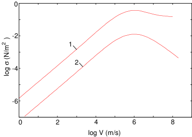
Figure 2: The velocity dependence of the frictional stress acting between two semi-infinite bodies at $d=10$nm (1) and $d=100$nm (2), with parameters chosen to correspond to copper ($\tau^{-1}=2.5\cdot 10^{13}$ s^-1, $\omega_{p}=1.6\cdot 10^{16}$ s^-1). (The base of the logarithm is 10)

The friction force acting on a small particle moving in parallel to a flat surface can be obtained from the friction between two semi-infinite bodies in the limit when one of the bodies is sufficiently rarefied. For $d\ll\lambda_{T}=c\hbar/k_{B}T$, in Eq. (22) we can neglect by the first term and in the second term we can integrate over the whole $q$-plane, and put $k_{z}\approx iq$. We will assume that the rarefied body consists of small metal particles which have the electric dipole moment and the magnetic moment. The dielectric permittivity and magnetic permeability of this body, say body 2, is close to the unity, i.e. $\varepsilon_{2}-1\rightarrow 4\pi n\alpha_{E}\ll 1$ and $\mu_{2}-1\rightarrow 4\pi n\alpha_{H}\ll 1$, where $n$ is the concentration of particles in body 2, $\alpha_{E}$ and $\alpha_{H}$ are their electric and magnetic susceptibilities. To linear order in the concentration $n$ the reflection amplitudes are

$$R_{2p}=\frac{\varepsilon_{2}k_{z}-\sqrt{\varepsilon_{2}\mu_{2}k^{2}-q^{2}}}{\varepsilon_{2}k_{z}+\sqrt{\varepsilon_{2}\mu_{2}k^{2}-q^{2}}}\approx\frac{\varepsilon_{2}-1}{\varepsilon_{2}+1}\approx 2\pi n\alpha_{E}$$

$$R_{2s}=\frac{\mu_{2}k_{z}-\sqrt{\varepsilon_{2}\mu_{2}k^{2}-q^{2}}}{\mu_{2}k_{z}+\sqrt{\varepsilon_{2}\mu_{2}k^{2}-q^{2}}}\approx\frac{\mu_{2}-1}{\mu_{2}+1}\approx 2\pi n\alpha_{H}$$

The friction force acting on a particle moving in parallel to a plane surface can be obtained as the ratio between the change of the frictional shear stress between two surfaces after displacement of body 2 by small distance $dz$, and the number of the particles in a slab with thickness $dz$:

$$F_{x}^{part}=\frac{d\sigma_{\|}(z)}{ndz}\Big{|}_{z=d}=\frac{2\hbar}{\pi^{2}}\int_{0}^{\infty}d\omega\int d^{2}q\frac{q_{x}q}{q^{2}-\beta^{2}q_{y}^{2}}e^{-2qd}\left(n_{2}(\omega^{\prime})-n_{1}(\omega)\right)$$

$$\times\left[q^{2}(\mathrm{Im}R_{p}\mathrm{Im}\alpha_{E}^{\prime}+\mathrm{Im}R_{s}\mathrm{Im}\alpha_{H}^{\prime})+\beta^{2}q_{y}^{2}(\mathrm{Im}R_{p}\mathrm{Im}\alpha_{H}^{\prime}+\mathrm{Im}R_{s}\mathrm{Im}\alpha_{E}^{\prime})\right]$$ (24)

where $\alpha_{E(H)}^{\prime}=\alpha_{E(H)}(\omega^{\prime})$. For a spherical particle with radius $R$ the electric and magnetic susceptibilities are given by LandauEl

$$\alpha_{E}=R^{3}\frac{\varepsilon-1}{\varepsilon+2}$$ (25)

$$\alpha_{H}=-\frac{R^{3}}{2}\left[1-\frac{3}{R^{2}\kappa^{2}}+\frac{3}{R\kappa}\cot{R\kappa}\right]$$ (26)

where $\kappa=k\sqrt{\varepsilon}$. Fig. 3 shows the velocity-dependence of the friction force which acts on a small copper particle with $R=10$nm, moving above copper sample at $d=20$nm. The contributions from the electric dipole and magnetic moments are shown separately. At small velocities the contribution from the magnetic moment is seven orders of magnitude larger then the contribution from the electric dipole moment.

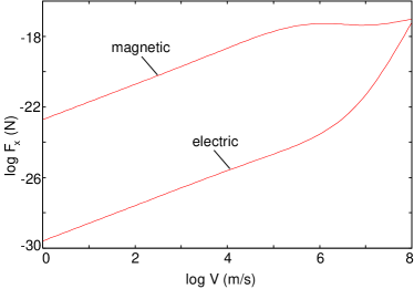
Figure 3: The velocity dependence of the friction force acting between small copper particle with radius $R=10$nm moving above a copper sample at the separation $d=20$nm. The contributions from the electric dipole moment and the magnetic moment are shown separately. (The base of the logarithm is 10)

IV Calculation of the conservative force between moving bodies

The $z$-component of the force is determined by $zz$-component of the Maxwell stress tensor:

$$\sigma_{zz}=-\frac{1}{4\pi}\int_{0}^{\infty}d\omega\int\frac{d^{2}q}{(2\pi)^{2}}\frac{k_{z}}{k^{2}}\left[(k_{z}+k_{z}^{*})(\left\langle\mid w_{p}\mid^{2}\right\rangle+\left\langle\mid w_{s}\mid^{2}\right\rangle\right.$$

$$\left.+\left\langle\mid v_{p}\mid^{2}\right\rangle+\left\langle\mid v_{s}\mid^{2}\right\rangle)+(k_{z}-k_{z}^{*})\left\langle(w_{p}v_{p}^{*}+w_{s}v_{s}^{*}+c.c\right\rangle\right]$$ (27)

One has to subtract the infinite vacuum contribution to the force which does not depend on separation $d$ Lifshitz54 ; Schwinger78 . Substituting (15-18) into Eq. (27) , and averaging over the fluctuating electromagnetic field with the help of Eq. (19), and after subtraction of the vacuum term, we get the $z$-component of the force:

$$F_{z}=\sigma_{zz}=-\frac{\hbar}{4\pi^{3}}\mathrm{Re}\int_{0}^{\infty}d\omega\int d^{2}q\frac{k_{z}}{\Delta}e^{2ik_{z}d}\Big{\{}(q^{2}-\beta kq_{x})^{2}[R_{1p}R_{2p}^{\prime}D_{ss}$$

$$+R_{1s}R_{2s}^{\prime}D_{pp}]-\beta^{2}k_{z}^{2}q_{y}^{2}[R_{1p}R_{2s}^{\prime}D_{sp}+R_{1s}R_{2p}^{\prime}D_{ps}]\Big{\}}[1+n_{1}(\omega)+n_{2}(\omega^{\prime})]$$

$$-\frac{\hbar}{16\pi^{3}}\int_{0}^{\infty}d\omega\int_{q<\omega/c}d^{2}q\frac{k_{z}}{|\Delta|^{2}}[(q^{2}-\beta kq_{x})^{2}+\beta^{2}k_{z}^{2}q_{y}^{2}]$$

$$\times\{(q^{2}-\beta kq_{x})^{2}[(1-\mid R_{1p}\mid^{2})(1+\mid R_{2p}^{\prime}\mid^{2})|D_{ss}|^{2}-(1\leftrightarrow 2,\omega\leftrightarrow\omega^{\prime})]$$

$$+\beta^{2}k_{z}^{2}q_{y}^{2}[(1-\mid R_{1p}\mid^{2})(1+\mid R_{2s}^{\prime}\mid^{2})|D_{sp}|^{2}-(1\leftrightarrow 2,\omega\leftrightarrow\omega^{\prime})]+(p\leftrightarrow s)\}\left(n_{1}(\omega)-n_{2}(\omega^{\prime})\right)$$

$$+\frac{\hbar}{4\pi^{3}}\int_{0}^{\infty}d\omega\int_{q>\omega/c}d^{2}q\frac{|k_{z}|}{|\Delta|^{2}}[(q^{2}-\beta kq_{x})^{2}+\beta^{2}k_{z}^{2}q_{y}^{2}]e^{-2\mid k_{z}\mid d}$$

$$\times\{(q^{2}-\beta kq_{x})^{2}[\mathrm{Im}R_{1p}\mathrm{Re}R_{2p}^{\prime}|D_{ss}|^{2}-(1\leftrightarrow 2,\omega\leftrightarrow\omega^{\prime})]-\beta^{2}k_{z}^{2}q_{y}^{2}[\mathrm{Im}R_{1p}\mathrm{Re}R_{2s}^{\prime}|D_{sp}|^{2}-(1\leftrightarrow 2,\omega\leftrightarrow\omega^{\prime})]$$

$$+(p\leftrightarrow s)\}\left(n_{1}(\omega)-n_{2}(\omega^{\prime})\right).$$ (28)

At $T_{1}=T_{2}=0$ K, Eq. (28) takes the form

$$F_{z}=-\frac{\hbar}{4\pi^{3}}\mathrm{Re}\left\{\int_{0}^{\infty}d\omega\int d^{2}q-\int_{-\infty}^{\infty}dq_{y}\int_{0}^{\infty}dq_{x}\int_{0}^{q_{x}V}d\omega\right\}\frac{k_{z}}{\Delta}e^{2ik_{z}d}$$

$$\Big{\{}(q^{2}-\beta kq_{x})^{2}[R_{1p}R_{2p}^{\prime}D_{ss}+R_{1s}R_{2s}^{\prime}D_{pp}]$$

$$-\beta^{2}k_{z}^{2}q_{y}^{2}[R_{1p}R_{2s}^{\prime}D_{sp}+R_{1s}R_{2p}^{\prime}D_{ps}]\Big{\}}$$

$$+\frac{\hbar}{4\pi^{3}}\int_{-\infty}^{\infty}dq_{y}\int_{0}^{\infty}dq_{x}\int_{0}^{q_{x}V}d\omega\frac{|k_{z}|}{|\Delta|^{2}}[(q^{2}-\beta kq_{x})^{2}+\beta^{2}k_{z}^{2}q_{y}^{2}]e^{-2\mid k_{z}\mid d}$$

$$\times\{(q^{2}-\beta kq_{x})^{2}[\mathrm{Im}R_{1p}\mathrm{Re}R_{2p}^{\prime}|D_{ss}|^{2}-(1\leftrightarrow 2,\omega\leftrightarrow\omega^{\prime})]-\beta^{2}k_{z}^{2}q_{y}^{2}[\mathrm{Im}R_{1p}\mathrm{Re}R_{2s}^{\prime}|D_{sp}|^{2}-(1\leftrightarrow 2,\omega\leftrightarrow\omega^{\prime})]$$

$$+(p\leftrightarrow s)\}\left(n_{1}(\omega)-n_{2}(\omega^{\prime})\right).$$ (29)

If in Eq. (28) one neglects the terms of the order $\beta^{2}$, then, as in the case of friction, the contributions from the waves with $p$- and $s$- polarization will be separated. In this case Eq. (28) reduces to

$$F_{z}=-\frac{\hbar}{4\pi^{3}}\mathrm{Re}\int_{0}^{\infty}d\omega\int d^{2}qk_{z}\left(\frac{1}{R_{1p}^{-1}R_{2p}^{\prime-1}e^{-2ik_{z}d}-1}\right.$$

$$\left.+\frac{1}{R_{1s}^{-1}R_{2s}^{\prime-1}e^{-2ik_{z}d}-1}\right)[1+n_{1}(\omega)+n_{2}(\omega^{\prime})]$$

$$-\frac{\hbar}{16\pi^{3}}\int_{0}^{\infty}d\omega\int_{q<\omega/c}d^{2}qk_{z}\Big{\{}\frac{[(1-\mid R_{1p}\mid^{2})(1+\mid R_{2p}^{\prime}\mid^{2})-(1\leftrightarrow 2,\omega\leftrightarrow\omega^{\prime})]}{|D_{pp}|2}$$

$$+(p\leftrightarrow s)\Big{\}}\left(n_{1}(\omega)-n_{2}(\omega^{\prime})\right)$$

$$+\frac{\hbar}{4\pi^{3}}\int_{0}^{\infty}d\omega\int_{q>\omega/c}d^{2}q|k_{z}|e^{-2\mid k_{z}\mid d}$$

$$\times\left\{\frac{[\mathrm{Im}R_{1p}\mathrm{Re}R_{2p}^{\prime}-(1\leftrightarrow 2,\omega\leftrightarrow\omega^{\prime})]}{|D_{pp}|^{2}}+(p\leftrightarrow s)\right\}\left(n_{1}(\omega)-n_{2}(\omega^{\prime})\right)$$ (30)

If we put $V=0$ and use the Fresnel’s formulas for the reflection amplitudes, then Eq. (30) reduces to the formula obtained by Lifshitz Lifshitz54 . Lifshitz have shown that at $T_{1}=T_{2}=0$ K it is convenient to transform $\omega$-integration along the real axis into the integral along the imaginary axis in the upper half of the complex $\omega$-plane. For a rarefied body, similarly as in Sec. III, for $d\ll\hbar/k_{B}T$ from (28) we get the van der Waals interaction between a small particle and plane surface:

$$F_{z}=\frac{\hbar}{\pi^{2}}\mathrm{Im}\int_{0}^{\infty}d\omega\int d^{2}q\frac{q^{2}e^{-2qd}}{q^{2}-\beta^{2}q_{y}^{2}}\Big{\{}q^{2}[R_{p}\alpha_{E}^{\prime}$$

$$+R_{s}\alpha_{H}^{\prime}]+\beta^{2}q_{y}^{2}[R_{p}\alpha_{H}^{\prime}+R_{s}\alpha_{E}^{\prime}]\Big{\}}[1+n_{1}(\omega)+n_{2}(\omega^{\prime})]$$

$$+\frac{\hbar}{\pi^{2}}\int_{0}^{\infty}d\omega\int d^{2}q\frac{q^{2}}{q^{2}-\beta^{2}q_{y}^{2}}e^{-2qd}$$

$$\times\{q^{2}[\mathrm{Im}R_{p}\mathrm{Re}\alpha_{E}^{\prime}-\mathrm{Re}R_{p}\mathrm{Im}\alpha_{E}^{\prime}]+\beta^{2}q_{y}^{2}[\mathrm{Im}R_{p}\mathrm{Re}\alpha_{H}^{\prime}-\mathrm{Im}R_{s}\mathrm{Re}\alpha_{E}^{\prime}]$$

$$+(p\leftrightarrow s,E\leftrightarrow H)\}\left(n_{1}(\omega)-n_{2}(\omega^{\prime})\right).$$ (31)

V Calculation of the radiative heat transfer between moving bodies

The radiative energy transfer between the bodies is determined by the ensemble average of the Poynting’s vector. In the case of two plane parallel surfaces the heat flux across the surface 1 is given by RMP07

$$\left\langle\mathbf{S}_{1z}(\mathbf{r})\right\rangle_{\omega}=(c/8\pi)\left\langle\mathbf{E}(\mathbf{r})\times\mathbf{B}^{*}(\mathbf{r})\right\rangle_{\omega}+c.c.$$

$$=\frac{ic^{2}}{8\pi\omega}\left\{\langle\mathbf{E}(\mathbf{r})\cdot\frac{d}{dz}\mathbf{E}^{*}(\mathbf{r})\rangle-c.c\right\}_{z=0}.$$ (32)

Using Eqs. (3,4) and (32) we get equations for the heat obtained by the body 1 which are very similar to Eq. (21) and (22):

$$S_{1}=\frac{1}{4\pi}\int_{0}^{\infty}d\omega\int\frac{d^{2}q}{(2\pi)^{2}}\frac{\omega}{k^{2}}\left[(k_{z}+k_{z}^{*})(\left\langle\mid w_{p}\mid^{2}\right\rangle+\left\langle\mid w_{s}\mid^{2}\right\rangle\right.$$

$$\left.-\left\langle\mid v_{p}\mid^{2}\right\rangle-\left\langle\mid v_{s}\mid^{2}\right\rangle)+(k_{z}-k_{z}^{*})\left\langle(w_{p}v_{p}^{*}+w_{s}v_{s}^{*}-c.c\right\rangle\right].$$ (33)

After averaging of the product of the components of the fluctuating electromagnetic field in the same way as in Sec. (III) we get

$$S_{1}=\frac{\hbar}{8\pi^{3}}\int_{0}^{\infty}d\omega\int_{q<\omega/c}d^{2}q\frac{\omega}{|\Delta|^{2}}[(q^{2}-\beta kq_{x})^{2}+\beta^{2}k_{z}^{2}q_{y}^{2}]$$

$$\times[(q^{2}-\beta kq_{x})^{2}(1-\mid R_{1p}\mid^{2})(1-\mid R_{2p}^{\prime}\mid^{2})|D_{ss}|^{2}$$

$$+\beta^{2}k_{z}^{2}q_{y}^{2}(1-\mid R_{1p}\mid^{2})(1-\mid R_{2s}^{\prime}\mid^{2})|D_{sp}|^{2}+(p\leftrightarrow s)]\left(n_{2}(\omega^{\prime})-n_{1}(\omega)\right)$$

$$+\frac{\hbar}{2\pi^{3}}\int_{0}^{\infty}d\omega\int_{q>\omega/c}d^{2}q\frac{\omega}{|\Delta|^{2}}[(q^{2}-\beta kq_{x})^{2}+\beta^{2}k_{z}^{2}q_{y}^{2}]e^{-2\mid k_{z}\mid d}$$

$$\times[(q^{2}-\beta kq_{x})^{2}\mathrm{Im}R_{1p}\mathrm{Im}R_{2p}^{\prime}|D_{ss}|^{2}-\beta^{2}k_{z}^{2}q_{y}^{2}\mathrm{Im}R_{1p}\mathrm{Im}R_{2s}^{\prime}|D_{sp}|^{2}$$

$$+(p\leftrightarrow s)]\left(n_{2}(\omega^{\prime})-n_{1}(\omega)\right).$$ (34)

Eq. (34) generalizes the equations for the heat transfer between two surfaces which are at the rest in the $K$-reference frame Polder ; Volokitin01a , to the case when the surfaces are moving relative to each other. There is also the heat $S_{2}$ obtained by the body 2 in the $K^{\prime}$-reference frame. Actually, $S_{1}$ and $S_{2}$ are the same quantities, looked at from different coordinate systems. These quantities are related by the equation:

$$F_{x}V=S_{1}+S_{2}/\gamma.$$ (35)

For the limiting case of rarefied body, similarly as in Sec. III, from (34) we get the contribution from evanescent waves to the heat adsorbed by a semi-infinite solid at $d\ll\lambda_{T}$ in the $K$-reference frame:

$$S=\frac{2\hbar}{\pi^{2}}\int_{0}^{\infty}d\omega\int d^{2}q\frac{q\omega}{q^{2}-\beta^{2}q_{y}^{2}}e^{-2qd}\left(n_{2}(\omega^{\prime})-n_{1}(\omega)\right)$$

$$\times\left[q^{2}(\mathrm{Im}R_{p}\mathrm{Im}\alpha_{E}^{\prime}+\mathrm{Im}R_{s}\mathrm{Im}\alpha_{H}^{\prime})+\beta^{2}q_{y}^{2}(\mathrm{Im}R_{p}\mathrm{Im}\alpha_{H}^{\prime}+\mathrm{Im}R_{s}\mathrm{Im}\alpha_{E}^{\prime})\right]$$ (36)

The heat adsorbed by a particle can be determined from Eq. (35).

VI Calculation of the friction force on a small neutral particle moving relative to black body radiation

We consider a small neutral particle moving relative to black body radiation. We introduce two reference frame $K$ and $K^{\prime}$. The thermal radiation is in equilibrium in the $K$-reference frame and the particle is at rest in the $K^{\prime}$-reference frames. We assume that the particle moves with velocity $V$ along the $x$-axis. The relation between the $x$-components of the momentum in the different reference frames is given by

$$p_{x}=(p_{x}^{\prime}+\beta E_{0}/c)\gamma$$ (37)

where $E_{0}$ is the rest energy of the particle. The rest energy can change due to thermal radiation of the particle. From Eq. (37) we get

$$\frac{dp_{x}}{dt}=\frac{dp_{x}^{\prime}}{dt^{\prime}}+\frac{V}{c^{2}}\frac{dE_{0}}{dt^{\prime}}$$ (38)

According to the Einstein law

$$\frac{dm_{0}}{dt^{\prime}}=\frac{1}{c^{2}}\frac{dE_{0}}{dt^{\prime}}$$ (39)

where $m_{0}$ is the rest mast of the particle. Taking into account that

$$\frac{dp_{x}}{dt}=\frac{d(m_{0}V\gamma)}{dt}=\frac{dm_{0}}{dt^{\prime}}V+m_{0}\frac{d(V\gamma)}{dt}$$ (40)

from Eqs. (38-40) we get

$$m_{0}\frac{d(V\gamma)}{dt}=\frac{dp_{x}^{\prime}}{dt^{\prime}}$$ (41)

In the rest reference frame, due to symmetry, the total radiated momentum from the dipole and magneto-dipole radiation is identically zero. Thus, the change of momentum of the particle in the rest reference frame is determined by the Lorenz force $F_{x}^{\prime}$ acting on the particle from the external electromagnetic field associated with the thermal radiation observed in this reference frame. The dynamics of the particle in the $K$-reference frame is determined by the equation

$$m_{0}\frac{d(V\gamma)}{dt}=F_{x}^{\prime}$$ (42)

Eq. (42) does not contain force from the thermal electromagnetic field radiated by the particle. Thus, from Eq. (42) it follows that, contrary to the claim of the authors of Dedkov05 , the thermal radiation of the particle can not produce any acceleration. In the $K^{\prime}$-reference frame the Lorenz force on the particle is determined by the expression Volokitin02 ; Dedkov08

$$F_{x}^{\prime}=\frac{\partial}{\partial x^{\prime}}\langle\mathbf{p_{e}^{\prime}\cdot E^{\prime*}(r^{\prime})}\rangle_{\mathbf{r^{\prime}=r^{\prime}_{0}}}+\frac{\partial}{\partial x^{\prime}}\langle\mathbf{p_{m}^{\prime}\cdot B^{\prime*}(r^{\prime})}\rangle_{\mathbf{r^{\prime}=r^{\prime}_{0}}}$$ (43)

Writing the electromagnetic field as a Fourier integral, and taking into account that

$$\mathbf{p}_{e}^{\prime}=\alpha_{E}(\omega^{\prime})\mathbf{E}^{\prime}(\mathbf{r^{\prime}_{0}})e^{-i\omega^{\prime}t^{\prime}},$$

$$\mathbf{p}_{m}^{\prime}=\alpha_{H}(\omega^{\prime})\mathbf{B}^{\prime}(\mathbf{r^{\prime}_{0}})e^{-i\omega^{\prime}t^{\prime}},$$

we get

$$F_{x}^{\prime}=-i\int_{\infty}^{\infty}\frac{d\omega^{\prime}}{2\pi}\int\frac{d^{3}k^{\prime}}{(2\pi)^{3}}k_{x}^{\prime}\left[\alpha_{E}(\omega^{\prime})\langle\mathbf{E^{\prime}\cdot E^{\prime*}}\rangle_{\omega^{\prime}\mathbf{k}^{\prime}}+\alpha_{H}(\omega^{\prime})\langle\mathbf{B^{\prime}\cdot B^{\prime*}}\rangle_{\omega^{\prime}\mathbf{k}^{\prime}}\right]$$

$$=-i\int_{\infty}^{\infty}\frac{d\omega^{\prime}}{2\pi}\int\frac{d^{3}k^{\prime}}{(2\pi)^{3}}k_{x}^{\prime}\left[\alpha_{E}(\omega^{\prime})+\alpha_{H}(\omega^{\prime})\right]\langle\mathbf{E^{\prime}\cdot E^{\prime*}}\rangle_{\omega^{\prime}\mathbf{k}^{\prime}}$$ (44)

where we have taken into account that for plane waves $\langle\mathbf{E^{\prime}\cdot E^{\prime*}}\rangle_{\omega^{\prime}\mathbf{k}^{\prime}}=\langle\mathbf{B^{\prime}\cdot B^{\prime*}}\rangle_{\omega^{\prime}\mathbf{k}^{\prime}}$. When we change from the $K^{\prime}$-reference frame to the $K$-reference frame $\langle\mathbf{E^{\prime}\cdot E^{\prime*}}\rangle_{\omega^{\prime}\mathbf{k}^{\prime}}$ is transformed as the energy density of a plane electromagnetic field. From the law of transformation of the energy density of a plane electromagnetic field LandauField we get

$$\langle\mathbf{E^{\prime}\cdot E^{\prime*}}\rangle_{\omega^{\prime}\mathbf{k}^{\prime}}=\langle\mathbf{E\cdot E^{*}}\rangle_{\omega\mathbf{k}}\left(\frac{\omega^{\prime}}{\omega}\right)^{2}.$$ (45)

According to the theory of the fluctuating electromagnetic field Lifshitz80

$$\langle\mathbf{E\cdot E^{*}}\rangle_{\omega\mathbf{k}}=4\pi^{2}\hbar k\left\{\delta(\frac{\omega}{c}-k)-\delta(\frac{\omega}{c}+k)\right\}[1+2n(\omega)]$$ (46)

Taking into account the invariance of the square of the four-wave vector $(\omega/c)^{2}-k^{2}=(\omega^{\prime}/c)^{2}-k^{\prime 2}$ Eq. (46) can be rewritten in the form

$$\langle\mathbf{E\cdot E^{*}}\rangle_{\omega\mathbf{k}}=\frac{4\pi^{2}\hbar k^{2}}{k^{\prime}}\left\{\delta(\frac{\omega^{\prime}}{c}-k^{\prime})-\delta(\frac{\omega^{\prime}}{c}+k^{\prime})\right\}[1+2n(\omega)]$$ (47)

Substitution Eqs. (45,47) in Eq. (44) and integration over $\omega^{\prime}$ gives

$$F_{x}=\frac{\hbar c}{2\pi^{2}}\int d^{3}kkk_{x}\left[\mathrm{Im}\alpha_{E}(ck)+\mathrm{Im}\alpha_{H}(ck)\right]$$

$$\times\left\{n[\gamma(ck+Vk_{x})]-n[\gamma(ck-Vk_{x})]\right\},$$ (48)

where we have omitted index of prime and have taken into account that $\omega=(\omega^{\prime}+k^{\prime}_{x}V)\gamma$. Introducing the new variable $\omega=ck$, (48) can be transformed to the form

$$F_{x}=\frac{2\hbar}{\pi c^{2}}\int_{0}^{\infty}d\omega\omega^{2}\int_{0}^{\omega/c}dk_{x}k_{x}\left[\mathrm{Im}\alpha_{E}(\omega)+\mathrm{Im}\alpha_{H}(\omega)\right]$$

$$\times\left\{n[\gamma(ck+Vk_{x})]-n[\gamma(ck-Vk_{x})]\right\}$$ (49)

Eq. (49) generalizes the result obtained in Mkrtchian to the case of large velocities, and includes the contribution from the magnetic moment. For metallic particles the contribution from the magnetic moment exceeds substantially the contribution from the electric dipole moment. At small velocities $F_{x}=-\Gamma V$, where

$$\Gamma=\frac{4\hbar}{3\pi c^{5}}\int_{0}^{\infty}d\omega\left(-\frac{\partial n}{\partial\omega}\right)\omega^{5}[\mathrm{Im}\alpha_{E}(\omega)+\mathrm{Im}\alpha_{H}(\omega)]$$ (50)

For metals with $4\pi\sigma\gg k_{B}T/\hbar$ and for $c\sqrt{2\pi\sigma k_{B}T}\gg R$, where $\sigma$ is the conductivity, from Eqs. (25) and (26) we get

$$\mathrm{Im}\alpha_{E}(\omega)\approx R^{3}\frac{3\omega}{4\pi\sigma}$$ (51)

$$\mathrm{Im}\alpha_{H}(\omega)=\frac{4\pi\sigma\omega R^{5}}{30c^{2}}$$ (52)

Setting the friction coefficient $\Gamma$ to $m_{0}/\tau$, where $\tau$ the relaxation time, and using $m_{0}=4\pi R^{3}\rho/3$, from Eqs. (50 -52) we get

$$\tau^{-1}_{e}\approx 10^{2}\frac{\hbar}{\rho\lambda_{T}^{5}}\frac{k_{B}T}{\hbar\sigma}$$ (53)

$$\tau^{-1}_{m}\approx 10^{2}\frac{\hbar R}{\rho\lambda_{T}^{6}}\frac{\sigma R}{c}$$ (54)

where $\tau_{e}^{-1}$ and $\tau_{m}^{-1}$ are the contributions to the friction from the electric dipole and magnetic moments, respectively. For $T=300$ K, $\rho\approx 10^{4}$ kg/m³, $\sigma\approx 10^{18}$ s^-1 from Eqs. (51,54) we get $\tau_{e}\sim 10^{16}$ s and $\tau_{m}\sim 10^{12}$ s. When the conductivity decreases $\tau_{e}$ also decreases and reaches minimum at $2\pi\sigma\approx k_{B}T/\hbar$. At $T=3000$ K this minimum corresponds to about a day ($\tau_{e}^{min}\approx 10^{5}$ s). In Mkrtchian the same relaxation time was obtained for $Ba^{+}$.

VII Conclusion

In this paper within the framework of unified approach we have calculated the Casimir-Lifshitz interaction, the van der Waals friction force and the radiative heat transfer at nonequilibrium conditions, when the interacting bodies are at different temperatures, and they move relative to each other with the arbitrary velocity $V$. In comparison with the existing literature we have studied more general nonequilibrium conditions. Our study was focused on the surface-surface and surface-particle configuration. We have found the exact solution of problem about the determination of the fluctuating electromagnetic field in the vacuum gap between two flat parallel surfaces moving relative to each other. Knowing the electromagnetic field we have calculated the Maxwell stress tensor and the Poynting vector which determine the friction and conservative forces, and the heat transfer between the solids, respectively. For the heat transfer and the conservative force our treatment generalizes the results obtained for bodies at rest to the case of bodies which move relative to each other. We have found that the velocity dependence of the considered phenomena is determined by Doppler shift and can be strong for resonant photon tunneling between the surface modes. This effect can be used for the precision determination of energy of the surface modes. We have shown that relativistic effects produce a mixing of the $s$ and $p$-wave contributions to the forces and the heat transfer. This relativistic effect is of the order $(V/c)^{2}$. If one neglects by terms of order $(V/c)^{2}$, the different polarizations will contribute to the forces and the heat transfer separately. The velocity dependence of the conservative force is much weaker than the velocity dependence of the friction force and the heat transfer. For the conservative force the important range of the frequencies is determined by the plasma frequency $\omega_{p}$ which is much larger than the Doppler shift $\Delta\omega=q_{x}V\sim V/d$ for practically all separations and velocities. Therefore the velocity dependent component of the Casimir-Lifshitz force will be considerably smaller than the $V=0$ component. The same is true for the thermal component of the Casimir-Lifshitz force. The thermal component was measured recently in Antezza05 . Thus, one can expect that the velocity dependent component also can be measured. For the friction force and the heat transfer the important range of the frequencies is determined by the thermal frequency $\omega_{T}=k_{B}T/\hbar$ which can be of the same order as the Doppler shift. The friction force initially increases when the velocity increases, reaches maximum at $V\sim\omega_{T}$, and then decreases. From the limit when one of the bodies is rarefied, we have calculated the interaction force and the heat transfer for a small particle outside a flat surface. For a particle we have taken into account the contribution to the forces and the heat transfer from the electric dipole and magnetic moments. For metallic particles we have found that the contribution to the friction from the magnetic moment exceeds the contribution from the electric dipole moment by several orders of magnitude. We have presented a relativistic theory of the friction force acting on a particle moving relative to the black body radiation. We have shown that the thermal radiation of the particle does not produce any acceleration and that the friction force acting on the particle is determined by external electromagnetic field associated with the black body radiation. For a metallic particle moving relative to the black body radiation the friction force increases initially when the conductivity decreases, reaches maximum at $2\pi\sigma\approx\omega_{T}$, and then decreases.

A.I.V acknowledges financial support from the Russian Foundation for Basic Research (Grant N 08-02-00141-a) and DFG.

References

- (1) S. M. Rytov, Theory of Electrical Fluctuation and Thermal Radiation (Academy of Science of USSR Publishing, Moscow, 1953)
- (2) M. L. Levin, S. M. Rytov, Theory of eqilibrium thermal fluctuations in electrodynamics (Science Publishing, Moscow, 1967)
- (3) S. M. Rytov, Yu. A. Kravtsov, and V. I. Tatarskii, Principles of Statistical Radiophyics(Springer, New York.1989), Vol.3
- (4) E. M. Lifshitz, Zh. Eksp. Teor. Fiz. 29 94 (1955) [Sov. Phys.-JETP 2 73 (1956)]
- (5) D. Polder and M. Van Hove, Phys. Rev. B 4, 3303 (1971)
- (6) A. I. Volokitin and B. N. J. Persson, J.Phys.: Condens. Matter 11, 345 (1999);Phys.Low-Dim.Struct.7/8,17 (1998)
- (7) M. Antezza, L. P. Pitaevskii, S. Stringari, and V. B. Svetovoy, Phys. Rev. A 77, 022901 (2008)
- (8) M. Antezza, L. P. Pitaevskii, and S. Stringari, Phys. Rev. Lett. 95, 113202 (2005)
- (9) M. Antezza, L. P. Pitaevskii, S. Stringari, and V. B. Svetovoy, and Phys. Rev. Lett. 97, 223203 (2006)
- (10) J. B. Pendry, J.Phys.:Condens.Matter 11, 6621 (1999).
- (11) A. I. Volokitin and B. N. J. Persson, Phys. Rev. B 63, 205404 (2001); Phys. Low-Dim. Struct. 5/6, 151 (2001)
- (12) A. I. Volokitin and B. N. J. Persson, Phys. Rev. B 69, 045417 (2004)
- (13) A. I. Volokitin and B. N. J.Persson, JETP Lett. 78 , 457(2003)
- (14) J. P. Mulet, K. Joulin, R. Carminati, and J. J. Greffet, Appl. Phys.Lett. 78, 2931 (2001)
- (15) J. P. Mulet, K. Joulain, R. Carminati, and J. J. Greffet, Microscale Thermophysical Engineering, 6(3), 209 (2002)
- (16) A. Kittel, W. Müller-Hirsch, J. Parisi, S. Biehs, D. Reddig, and M. Holthaus, Phys. Rev. Lett. 95, 224301 (2005).
- (17) K. Joulain, J. P. Mulet, F. Marquier, R. Carminati, and J. J. Greffet, Surf. Sci. Rep. , 57, 59 (2005)
- (18) A. I. Volokitin and B. N. J. Persson, Rev. Mod. Phys. 79, 1291 (2007)
- (19) A. I. Volokitin and B. N. J. Persson, J.Phys.: Condens. Matter 13, 859 (2001)
- (20) A. I. Volokitin and B. N. J. Persson, Phys. Rev. Lett. 91, 106101 (2003).
- (21) A. I. Volokitin and B. N. J. Persson, Phys. Rev. B, 68, 155420 (2003).
- (22) V. Mkrtchian, V. A. Parsegian, R. Podgornik, and W. M. Saslow, Phys. Rev. Lett. 91, 220801 (2003)
- (23) P.-O. Chapius, M. Laroche, S. Volz, and J.-J. Greffet, Phys. Rev. 77, 125402 (2008)
- (24) J. B. Pendry, J. Phys. C9 10301 (1997).
- (25) L. D. Landau and E. M. Lifshitz, Electrodynamics of Continuous Media, Pergamon, Oxford, 1960.
- (26) J. Schwinger, L. DeRaad, K. Milton, Ann. Phys. 115, 1 (1978)
- (27) G. V. Dedkov, A. A. Kyasov, Phys. Lett. A 339, 212 (2005)
- (28) A. I. Volokitin and B. N. J. Persson, Phys. Rev. B 65, 115419 (2002)
- (29) G. V. Dedkov, A. A. Kyasov, Tech. Phys. 53, 389 (2008)
- (30) L. D. Landau and E. M. Lifshitz, The classical theory of field, Pergamon, Oxford, 1975.
- (31) E. M. Lifshitz and L. P. Pitaevskii, Statistical Physics, Pt.2 Pergamon, Oxford, 1980.