Bayesian Analysis of Marginal Log-Linear Graphical Models for Three Way Contingency Tables

Abstract

This paper deals with the Bayesian analysis of graphical models of marginal independence for three way contingency tables. We use a marginal log-linear parametrization, under which the model is defined through suitable zero-constraints on the interaction parameters calculated within marginal distributions. We undertake a comprehensive Bayesian analysis of these models, involving suitable choices of prior distributions, estimation, model determination, as well as the allied computational issues. The methodology is illustrated with reference to two real data sets.

Keywords: Graphical models, Marginal log-linear parametrization, Model selection, Monte Carlo computation, Order decomposability, Power prior.

1 Introduction

Graphical models of marginal independence were originally introduced by Cox and Wermuth (1993) for the analysis of multivariate Gaussian distributions. They compose a family of multivariate distributions incorporating the marginal independences represented by a bidirected graph. The nodes in the graph correspond to a set of random variables and the bidirected edges represent the pairwise associations between them. A missing edge from a pair of nodes indicates that the corresponding variables are marginally independent. The complete list of marginal independences implied by a bidirected graph were studied by Kauermann (1996) and by Richardson (2003) using the so-called Markov properties.

The analysis of the Gaussian case can be easily performed both in classical and Bayesian frameworks since marginal independences correspond to zero constraints in the variance-covariance matrix. The situation is more complicated in the discrete case, where marginal independences correspond to non linear constraints on the set of parameters. Only recently parameterizations for these models have been proposed by Lupparelli (2006), Lupparelli et al. (2008) and Drton and Richardson (2008). In this paper we use the parameterization proposed by Lupparelli (2006) and Lupparelli et al. (2008) based on the class of marginal log-linear models of Bergsma and Rudas (2002). Each log-linear parameter is calculated within the appropriate marginal distribution and a graphical model of marginal independence is defined by zero constraints on specific higher order log-linear parameters. Alternative parameterizations have been proposed by Drton and Richardson (2008) based on the Moebius inversion and by Lupparelli et al. (2008) based on multivariate logistic representation of the models of Glonek and McCullagh (1995).

We present a comprehensive Bayesian analysis of discrete graphical models of marginal independence, involving suitable choices of prior distributions, estimation, model determination as well as the allied computational issues. Here we focus on the three way case where the joint probability of each model under consideration can be appropriately factorized. We work directly in terms of the vector of joint probabilities on which we impose the constraints implied by the graph. Then we consider a minimal set of probability parameters expressing marginal/conditional independences and sufficiently describe the graphical model of interest. We introduce a conjugate prior distribution based on Dirichlet priors on the appropriate probability parameters. The prior distribution factorize similarly to the likelihood. In order to make the prior distributions ‘compatible’ across models we define all probability parameters (marginal and conditional ones) of each model from the parameters of the joint distribution of the full table. In order to specify the prior parameters of the Dirichlet prior distribution, we adopt ideas based on the power prior approach of Ibrahim and Chen (2000) and Chen et al. (2000).

The plan of the paper is as follows. In Section 2 we introduce graphical models of marginal independence, we establish the notation, we present Markov properties and we explain in detail their log-linear parameterization. Section 3 illustrates a suitable factorization of the likelihood function for all models of marginal independence in three-way tables. In Section 4, we consider conjugate prior distributions, we present an imaginary data approach for prior specification and we compare alternative prior set-ups. Section 5 provides posterior model and parameter distributions which can be easily calculated via conjugate analysis. Two illustrative examples are presented in Section 6. Finally, we end up with a discussion and some final comments regarding our current research on the topic.

2 Preliminaries

2.1 Graphical Models of Marginal Independence

A bidirected graph $G=\left(\mathcal{V},E\right)$ is characterized by a vertex set ${\mathcal{V}}$ and an edge set $E$ with the property that $(v_{i},v_{j})\in E$ if and only if $(v_{j},v_{i})\in E$. We denote each bidirected edge by $(\overleftrightarrow{v_{i},v_{j}})=\big{\{}(v_{i},v_{j}),\,(v_{j},v_{i})\big{\}}$ and we represent it with a bidirected arrow. If a vertex $v_{i}$ is adjacent to another vertex $v_{j}$, then $v_{j}$ is said to be spouse of $v_{i}$, and we write $v_{j}\in sp(v_{i})$. For a set $A\subseteq{\cal V}$, we define $sp(A)=\cup\left(sp(v)|v\in A\right)$. The degree $d(v)$ of a vertex $v$ is the cardinality of the spouse set. A path connecting two vertices, $v_{0}$ and $v_{m}$, is a finite sequence of distinct vertices $v_{0},\ldots v_{m}$ such that $(v_{i-1},v_{i}),\;i=1,\ldots,m$, is an edge of the graph. A vertex set $C\subseteq{\mathcal{V}}$ is connected if every two vertexes $v_{i}$ and $v_{j}$ are joined by a path in which every vertex is in C. Two sets $A,B\in\mathcal{V}$ are separated by a third set $S\in\mathcal{V}$ if any path from a vertex in A to a vertex in $B$ contains a vertex in $S$. It can be shown that, if a subset of the nodes $D$ is not connected then there exist a unique partition of it into maximal (with respect to inclusion) connected set $C_{1},\ldots,C_{r}$

$$D=C_{1}\cup C_{2}\cup\ldots\cup C_{r}.$$ (1)

The graph is used to represent marginal independences between a set of discrete random variables $X_{\cal V}=\big{(}X_{v},~{}v\in{\cal V}\big{)}$, each one taking values $i_{v}\in{\cal I}_{v}$. The cross-tabulation of variables $X_{\cal V}$ produces a contingency table of dimension $|{\cal V}|$ with cell frequencies ${\mbox{\boldmath$n$}}=\Big{(}n(i),~{}i\in{\cal I}\Big{)}$ where ${\cal I}=\times_{v\in{\cal V}}{\cal I}_{v}$. Similarly for any marginal $M\subseteq{\cal V}$, we denote with $X_{M}=\big{(}X_{v},~{}v\in M\big{)}$ the set of variables which produce the marginal table with frequencies ${\mbox{\boldmath$n$}}_{M}=\Big{(}n_{M}(i_{M}),~{}i_{M}\in{\cal I}_{M}\Big{)}$ where ${\cal I}_{M}=\times_{v\in M}{\cal I}_{v}$. The marginal cell counts are the sum of specific elements of the full table and are given by

$$n_{M}(i_{M})=\sum_{j\in{\cal I}_{\overline{M}|i_{M}}}n(j)$$

where $\overline{M}={\cal V}\setminus M$ and ${\cal I}_{\overline{M}|i_{M}}=\{j\in{\cal I}:j_{M}=i_{M}\}$. Therefore ${\cal I}_{\overline{M}|i_{M}}$ refers to all cells of the full table for which the variables of the $M$ marginal are constrained to the specific value $i_{M}$.

A graphical model of marginal independence is constructed via the following Markov properties.

Definition 1

: Connected Set Markov Property (Richardson, 2003). The distribution of a random vector $X_{\cal V}$ is said to satisfy the connected set Markov property if

$$X_{C}\bot\bot X_{\mathcal{V}\setminus(C\cup sp(C))}$$ (2)

whenever $\emptyset\neq C\subseteq{\cal V}$ is a connected set.

A more exhaustive Markov property is the global Markov property, which requires all the marginal independences in (2), but also additional conditional independences.

Definition 2

: Global Markov Property (Kauermann, 1996 and Richardson, 2003). The distribution of a random vector $X_{\cal V}=\{X_{v},v\in{V}\}$ satisfies the Global Markov property if

$$A~{}\mbox{is separated from}~{}B~{}\mbox{by}~{}V\setminus(A\cup B\cup C)~{}\mbox{in}~{}G~{}\mbox{implies}~{}X_{A}\bot\bot X_{B}|X_{C},$$ (3)

with $A$, $B$ and $C$ disjoint subsets of $V$, and C may be empty.

Despite the global Markov property is more exhaustive (in the sense that indicates both marginal and conditional independences), Drton and Richardson (2008) pointed out that a distribution satisfies the global Markov property if and only if it satisfies the connected set Markov property.

¿From the global Markov property, we directly derive that if two nodes $i$ and $j$ are disconnected, then $X_{i}\bot\bot X_{j}$ that is the variables are marginal independent. The same is true for any two sets $A\subset{\cal V}$ and $B\subset{\cal V}$ that are disconnected, implying that $A\bot\bot B$ (are marginal independent). This can be easily generalized for any given disconnected set $D$ satisfying (1). Then the global Markov property for the bidirected graph $G$ implies

$$X_{C_{1}}\bot\bot X_{C_{2}}\bot\bot\ldots\bot\bot X_{C_{r}}.$$

According to Drton and Richardson (2008), a discrete marginal graphical model, associated to a bidirected graph G, is a family $P(G)$ of joint distributions for a categorical random vector $X_{\cal V}$ satisfying the global Markov property (or equivalently the connected set Markov property). Following the above, for every not connected set $D\subseteq{\cal V}$, it holds that

$$P(X_{D}=i_{D})=\prod_{k=1}^{r}P(X_{C_{k}}=i_{C_{k}})$$ (4)

where $C_{1},\ldots,C_{r}$ are the inclusion maximal connected sets satisfying (1).

2.2 A Parameterization for Marginal Log-Linear Models

Lupparelli (2006) and Lupparelli et al. (2008) show that it is possible to define a parameterization for any set $X_{\cal V}$ of categorical variables, by using the marginal log-linear model by Bersgma and Rudas (2002).

Bergsma and Rudas (2002) suggested to work in terms of log-linear parameters $\lambda$ obtained from a specific set of marginal tables. They consider the following model

$$\mbox{\boldmath$\lambda$}=\mbox{\boldmath$C$}\log\Big{(}\mbox{\boldmath$M$}\mbox{vec}(\mbox{\boldmath$\pi$})\Big{)}$$ (5)

where ${\mbox{\boldmath$\pi$}}=\Big{(}\pi(i),~{}i\in{\cal I}\Big{)}$ is the joint probability distribution of $X_{\cal V}$ and $\mbox{vec}(\mbox{\boldmath$\pi$})$ is a vector of dimension $|{\cal I}|$ obtained by rearranging the elements $\pi$ in a reverse lexicographical ordering of the corresponding variable levels with the level of the first variable changing first (or faster). For example in a $2\times 2$ table the vector of probabilities will be given by $\mbox{vec}(\mbox{\boldmath$\pi$})=\Big{(}\pi(1,1),\pi(2,1),\pi(1,2),\pi(2,2)\Big{)}^{T}$. In this paper we assume that the parameter vector $\lambda$ satisfies sum-to-zero constraints and we indicate with $C$ the corresponding contrast matrix. Finally $M$ is the marginalization matrix which specifies from which marginal we calculate each element of $\lambda$. An algorithm for constructing $C$ and $M$ matrices is given in the Appendix ( for additional details see Appendix A in Lupparelli, 2006).

2.2.1 Properties of Marginal Log-Linear Parameters

Let $M\subseteq{\cal V}$ be a generic marginal, and indicate with $S({M})$ the class of all subsets of ${M}$ and with $\mbox{\boldmath$\cal E$}_{M}\in S({M})$ the set of effects obtained from marginal $M$.

Given ${\cal M}=\{M_{1},M_{2},\dots,M_{|{\cal M}|}\}$ the set of marginals used to calculate the log-linear parameters $\lambda$, we denote by $\mbox{\boldmath$\lambda$}_{\mbox{\it{\Large e}}}^{M}=\Big{(}\mbox{\boldmath$\lambda$}_{\mbox{\it{\Large e}}}^{M}(i_{\mbox{\it{\Large e}}}),~{}i_{\mbox{\it{\Large e}}}\in{\cal I}_{\mbox{\it{\Large e}}},~{}M\in{\cal M}\Big{)}$, the set of parameters for effect $\mbox{\it{\Large e}}\subseteq M$ estimated by the marginal $M$ and by $\mbox{\boldmath$\lambda$}^{M}$ the set of all parameters estimated by the same marginal.

According to Bersgma and Rudas (2002), in order to obtain a well-defined parameterization, it is important to allocate the interaction parameters $\lambda$ among the chosen marginals to get a complete and hierarchical set of parameters.

Definition 3

: Complete and hierarchical set of parameters. A set of marginal log-linear parameters $\lambda$ is called hierarchical and complete if:

• The elements of ${\cal M}$ are ordered in a non decreasing order, which means that no marginal is a subset of any preceding one, i.e. ${M}_{i}\not\subseteq{M}_{j}\;\;\mbox{if~{}~{}}i>j$ (hierarchical ordering).

  Furthermore, we require the last marginal in the sequence to be the set all vertices under consideration, therefore $M_{|{\cal M}|}={\cal V}$ .

• From each marginal ${M}_{i}$ we can calculate only the effects that was not possible to get from the ones preceding it in the ordering under consideration; hence the sets ${\cal E}_{M_{i}}$ of the effects under consideration are given by

  $${\cal E}_{M_{1}}=S({M}_{1})\;\;\mbox{and}\;\;{\cal E}_{M_{i}}=S({M}_{i})\setminus\left\{\cup_{k=1}^{i-1}S({M}_{k})\right\}\;\mbox{for}\;\;i=1,\ldots,|{\mathbb{M}}|~{}.$$

The above set of parameters define a parametrization of the distribution on the contingency table (see Bergsma and Rudas, 2002, for a formal definition). It is called complete since each parameter is estimated from one and only one marginal and hierarchical because the full set of parameters is generated by marginals in a non decreasing ordering (Bersgma and Rudas, 2002, p 143-144).

For every complete and hierarchical set of parameters, the inverse transformation of (5) always exists but it cannot be analytically calculated (Lupparelli, 2006, p. 39). Iterative procedures have been used to calculate $\pi$ for any given values of $\lambda$ and hence the likelihood of the graph under consideration (Rudas and Bergsma, 2004 and Lupparelli, 2006).

An important problem when working with marginal log-linear parameters $\lambda$ is that we may end up with the definition of non-existing joint marginal probabilities. A way to avoid this is to consider the parameters’ variation independence property; see Bergsma and Rudas (2002). A set of parameters is variation independent when the range of possible values of one of them does not depend on the other’s value. Hence the joint range of the parameters is the Cartesian product of the separate ranges of the parameters involved. This property ensures the existence of a common joint distribution deriving from the marginals of the model under consideration. Moreover, variation independence ensures strong compatibility which implies both compatibility of the marginals and existence of a common joint distribution. Compatibility of the marginals means that from different distributions we will end up to the same distribution for the common parameters, for example from marginals AB and AC we get the same marginal for A. To assure variation independence of hierarchical log-linear parameters, a generalization of the classical decomposability concept is needed.

Definition 4

: Decomposable set of Marginals. A class of incomparable (with respect to inclusion) marginals ${\cal M}$ is called decomposable if it has at most two elements ($|{\cal M}|\leq 2$) or if there is an ordering ${M}_{1},\ldots,{M}_{|{\cal M}|}$ of its elements such that, for $k=3,\ldots,|{\cal M}|$ there exist at least one $j_{k}<k$ for which the running intersection property is satisfied, that is

$$\left(\cup_{i=1}^{k-1}{M}_{i}\right)\cap{M}_{k}={M}_{j_{k}}\cap{M}_{k}~{}.$$

Definition 5

: Ordered decomposable set of marginals. A class of marginals ${\cal M}$ is ordered decomposable if it has at most two elements or if there is a hierarchical ordering ${M}_{1},\ldots,{M}_{|{\cal M}|}$ of the marginals and, for $k=3,\ldots,|{\cal M}|$, the maximal elements (in terms of inclusion) of $\{{M}_{1},\ldots,{M}_{k}\}$ form a decomposable set.

The importance of the above property is due to the theorem 4 of Bergsma and Rudas (2002) where they proved that a set of complete and hierarchical marginal log-linear parameters is variation independent if and only if the ordering of the marginals involved is ordered decomposable. Hence order decomposability ensures the existence of a well defined joint probability.

2.3 Construction of Marginal Log-Linear Graphical Models

Based on the results of the previous subsection, Lupparelli (2006) and Lupparelli et al. (2008) proposed a strategy to construct a marginal log-linear parametrization for the family of discrete bidirected graphical.

Initially we need to consider a set of a parameters $\lambda$ derived from a hierarchical ordering of the marginals in ${\cal D}(G)\cup{\cal V}$; where ${\cal D}(G)$ is the set of all disconnected components of the bidirected graph ${G}$. Then, we must set the highest order log-linear interaction parameters of ${\cal D}(G)$ equal to zero.

More precisely, we need to consider the following steps:

1. Construct a hierarchical ordering of the marginals $M_{i}\in{\cal D}(G)$.

2. Append the marginal $M={\cal V}$ (corresponding to the full table under consideration) at the end of the list if it is not already included.

3. For every marginal table $M_{i}\in{\cal D}(G)\cup{\cal V}$ estimate all parameters of effects in $M_{i}$ that have not already estimated from the preceding marginals.

4. For every marginal table $M_{i}\in{\cal D}(G)$, set the highest order log-linear interaction parameter equal to zero; see Proposition 4.3.1 in Lupparelli (2006).

In the three way case the log-linear parameters the marginals are always obtained from a set of order of order decomposable marginals, hence the parameters are variation independent.

3 Likelihood Decomposition

In this paper we propose to use a different approach from the one by Rudas and Bergsma (2004) and Lupparelli (2006) in order to estimate the joint distribution $\pi$ of a graph $G$. We impose the constraints implied by the graph $G$ directly on the joint probabilities $\pi$. We work with a minimal set of probability parameters $\mbox{\boldmath$\pi$}^{G}$ expressing marginal/conditional independences and sufficiently describe the graphical model $G$ under investigation. By this way we can always reconstruct the joint distribution $\pi$ for a given graph $G$ via $\mbox{\boldmath$\pi$}^{G}$ and then simply calculate the marginal log-linear parameters directly using (5). Here we focus on the three way case where the joint probability of each model can be appropriately factorized for any graph $G$.

For every three way contingency table eight possible graphical models models exist which can be represented by four different types of graphs: the independence, the saturated, the edge and the gamma structure graph (see Figure 1). The independence graph is the one with the empty edge set ($E=\emptyset$), the saturated is the one containing all possible edges $\left[E=\big{(}\overleftrightarrow{(v,w)}:v\neq w\in{\cal V}\big{)}\right]$, an edge graph is the one having only one single edge and a gamma structure graph is one represented by a single path of length two. In a three way table, three ‘edge’ and three ‘gamma’ graphs are available.

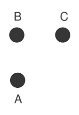
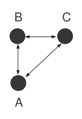
(a) Independence Model	(b) Saturated Model	(c) Edge Model	(d) Gamma Model

Figure 1: Type of Graphs in Three Way Tables

For the saturated model $G_{S}$, we get all parameters from the full table, i.e. $\mbox{\boldmath$\pi$}^{G_{S}}=\mbox{\boldmath$\pi$}$. Thus, the likelihood is directly written as

$$f(\mbox{\boldmath$n$}|\mbox{\boldmath$\pi$},G_{S})=\frac{\Gamma(N+1)}{\prod\limits_{i\in{\cal I}}\ \Gamma\Big{(}n(i)+1\Big{)}}\prod_{i\in{\cal I}}\pi(i)^{n(i)}$$

where $N=\sum_{i\in{\cal I}}n(i)$ is the total sample size.

The joint distributions for the independence and the edge models can be easily expressed using the equation

$$f(\mbox{\boldmath$n$}|\mbox{\boldmath$\pi$}^{G},G)=\frac{\Gamma(N+1)}{\prod\limits_{i\in{\cal I}}\ \Gamma\Big{(}n(i)+1\Big{)}}\prod_{d\in{\cal D}(G)}\;\prod_{i_{d}\in{\cal I}_{d}}\pi_{d}(i_{d})^{n(i_{d})}~{}$$

where $\mbox{\boldmath$\pi$}^{G}=\Big{(}\mbox{\boldmath$\pi$}_{d},\,d\in{\cal D}(G)\Big{)}$ and $\mbox{\boldmath$\pi$}_{d}=\Big{(}\pi_{d}(i_{d}),\,i_{d}\in{\cal I}_{d}\Big{)}$ is the vector of probabilities corresponding to the table of the marginal $d$. The above equation derives directly from (4) since the graph is disconnected.

Finally, the decomposition of the gamma structures is not as straightforward as in the previous case. In addition to specific marginal probability parameters we also need to use some conditional ones. Let us denote by “$c$” the corner node, that is the vertex with degree 2 and by $\overline{c}={\cal V}\setminus c$ the end-points of the path. The set of disconnected marginals is equal to the end-point vertices of the graph, hence $\overline{c}={\cal D}(G)$. Then the likelihood can be written as

$$f(\mbox{\boldmath$n$}|\mbox{\boldmath$\pi$}^{G},G)=\frac{\Gamma(N+1)}{\prod\limits_{i\in{\cal I}}\ \Gamma\Big{(}n(i)+1\Big{)}}\prod_{i_{\overline{c}}\;\in{\cal I}_{\overline{c}}}\left(\prod_{i_{c\in{\cal I}_{c}}}\pi_{c|\overline{c}}(i_{c}|i_{\overline{c}})^{n(i_{c},i_{\overline{c}})}\right)\left[\prod_{d\in{\cal D}(G)}\;\prod_{i_{d}\in{\cal I}_{d}}\pi_{d}(i_{d})^{n(i_{d})}\right]~{},$$

where $\mbox{\boldmath$\pi$}^{G}=\Big{(}\mbox{\boldmath$\pi$}_{c|\overline{c}},\,\mbox{\boldmath$\pi$}_{d},\,d\in{\cal D}(G)\Big{)}$, here ${\cal D}(G)={\cal V}\setminus c$ and

$$\mbox{\boldmath$\pi$}_{c|\overline{c}}=\Big{(}\pi_{c|\overline{c}}(i_{c}|i_{\overline{c}}),~{}i_{c}\in{\cal I}_{c},~{}i_{\overline{c}}\in{\cal I}_{\overline{c}}\Big{)}$$

are all the conditional probabilities of $c$ given $\overline{c}$.

The above factorization can be easily adopted to get maximum likelihood estimates analytically and avoid the iterative procedure used by Rudas and Bersgma (2004) and Lupparelli (2006). In this paper we work using conjugate priors on the appropriate probability parameters of the above parametrization and then calculate the corresponding log-linear parameters.

4 Prior distributions on cell probabilities

4.1 Conjugate Priors

For the specification of the prior distribution of the probability parameter vector we initially consider a Dirichlet distribution with parameters ${\mbox{\boldmath$\alpha$}}=\big{(}\alpha(i),\,i\in{\cal I}~{}\big{)}$ for the vector of the joint probabilities of the full table ${\mbox{\boldmath$\pi$}}=\big{(}\pi(i),\,i\in{\cal I}\big{)}$, where ${\cal I}$ is the set of all cells of the table under consideration. Hence, for the full table the prior density is given by

$$f({\mbox{\boldmath$\pi$}})=\frac{\varGamma(\alpha)}{\prod\limits_{i\in{\cal I}}\ \varGamma\Big{(}\alpha(i)\Big{)}}\prod_{i\in{\cal I}}\pi(i)^{\alpha(i)-1}=f_{{\cal D}i}(\mbox{\boldmath$\pi$};\,\mbox{\boldmath$\alpha$})$$ (6)

where $f_{{\cal D}i}\big{(}\mbox{\boldmath$\pi$};~{}\mbox{\boldmath$\alpha$}\big{)}$ is the density function of the Dirichlet distribution evaluated at $\pi$ with parameters $\alpha$ and $\alpha=\sum_{i\in{\cal I}}\alpha(i)$.

Under this set-up, the marginal prior of $\pi(i)$ is a Beta distribution with parameters $\alpha(i)$ and $\alpha-\alpha(i)$, i.e. $\pi(i)\sim Beta\Big{(}\alpha(i),\alpha-\alpha(i)\Big{)}$. The prior mean and variance of each cell is given by

$$E\big{[}\pi(i)\big{]}=\frac{\alpha(i)}{\alpha}\mbox{~{}~{}and~{}~{}}V\big{[}\pi(i)\big{]}=\frac{\alpha(i)\{\alpha-\alpha(i)\}}{\alpha^{2}(\alpha+1)}~{}.$$

When no prior information is available then we usually set all $\alpha(i)=\frac{\alpha}{|{\cal I}|}$ resulting to

$$E\big{[}\pi(i)\big{]}=\frac{1}{|{\cal I}|}\mbox{~{}~{}and~{}~{}}V\big{[}\pi(i)\big{]}=\frac{|{\cal I}|-1}{|{\cal I}|^{2}(\alpha+1)}~{}.$$

Small values of $\alpha$ increase the variance of each cell probability parameter. Usual choices for $\alpha$ are the values $|{\cal I}|/2$ (Jeffrey’s prior), $|{\cal I}|$ and $1$ (corresponding to $\alpha(i)$ equal to $1/2$, $1$ and $1/|{\cal I}|$ respectively); for details see Dellaportas and Forster (1999). The choice of this prior parameter value is of prominent importance for the model comparison due to the well known sensitivity of the posterior model odds and the Bartlett-Lindley paradox (Lindley, 1957, Bartlett, 1957). Here this effect is not so adverse, as for example in usual variable selection for generalized linear models, for two reasons. Firstly even if we consider the limiting case where $\alpha(i)=\frac{\alpha}{|{\cal I}|}$ with $\alpha\rightarrow 0$, the variance is finite and equal to $(|{\cal I}|-1)/|{\cal I}|^{2}$. Secondly, the distributions of all models are constructed from a common distribution of the full model/table making the prior distributions ‘compatible’ across different models (Dawid and Lauritzen, 2000 and Roverato and Consonni, 2004).

The model specific prior distributions are defined by the constraints imposed by the model’s graphical structure and the adopted factorization. The prior distribution also factorizes in same manner as the likelihood described in section 3. Thus, the prior for the saturated model is the usual Dirichlet (6).

For the independence and edge models the prior is given by

$$f\left(\mbox{\boldmath$\pi$}^{G}\big{|}G\right) = \prod_{d\in{\cal D}(G)}\;\left[\frac{\Gamma\left(\alpha\right)}{\prod\limits_{i_{d}\in{\cal I}_{d}}\ \Gamma\Big{(}\alpha(i_{d})\Big{)}}\prod_{i_{d}\in{\cal I}_{d}}\pi_{d}(i_{d})^{\alpha{(i_{d})-1}}\right]=\prod_{d\in{\cal D}(G)}\;f_{{\cal D}i}(\mbox{\boldmath$\pi$}_{d};~{}\mbox{\boldmath$\alpha$}_{d})$$

with parameter vector $\mbox{\boldmath$\pi$}^{G}=\big{(}\mbox{\boldmath$\pi$}_{d},\,d\in{\cal D}(G)\big{)}$. We denote the above density which is a simple product (over all disconnected sets) of Dirichlet distributions by

$$f\left(\mbox{\boldmath$\pi$}^{G}\right)=f_{\cal PD}\Big{(}\mbox{\boldmath$\pi$}_{d};~{}\mbox{\boldmath$\alpha$}_{d},\,d\in{\cal D}(G)\Big{)}.$$ (7)

For the gamma structure the prior is given by

$$p\left(\mbox{\boldmath$\pi$}^{G}\right) = \prod_{i_{\overline{c}}\;\in{\cal I}_{\overline{c}}}\left\{\frac{\Gamma\Big{(}\alpha(i_{\overline{c}})\Big{)}}{\prod\limits_{i_{c}\in{\cal I}_{c}}\ \Gamma\Big{(}\alpha(i_{c},i_{\overline{c}})\Big{)}}\left(\prod_{i_{c\in{\cal I}_{c}}}\pi_{c|\overline{c}}(i_{c},i_{\overline{c}})^{\alpha(i_{c},i_{\overline{c}})-1}\right)\right\}$$

$$\times ~{}f_{\cal PD}\Big{(}\mbox{\boldmath$\pi$}_{d};~{}\mbox{\boldmath$\alpha$}_{d},\,d\in{\cal D}(G)\Big{)}$$

with parameter vector $\mbox{\boldmath$\pi$}^{G}\big{(}\mbox{\boldmath$\pi$}_{c|\overline{c}},\,\mbox{\boldmath$\pi$}_{d},\,d\in{\cal D}(G)\big{)}$. The fist part of equation (4.1), that is the product for all level of $\overline{c}$ of Dirichlet distributions of the conditional probabilities, can be denoted by $f_{\cal CPD}\big{(}\mbox{\boldmath$\pi$}_{c|\overline{c}}\,;~{}\mbox{\boldmath$\alpha$}\big{)}$. Then, the prior density (4.1) can be written as

$$f\left(\mbox{\boldmath$\pi$}^{G}\right) = f_{\cal CPD}\big{(}\mbox{\boldmath$\pi$}_{c|\overline{c}}\,;~{}\mbox{\boldmath$\alpha$}\big{)}f_{\cal PD}\big{(}\mbox{\boldmath$\pi$}_{d};~{}\mbox{\boldmath$\alpha$}_{d},\,d\in{\cal D}(G)\big{)}~{}.$$ (9)

In order to make the prior distributions ‘compatible’ across models, we define the prior parameters of $\mbox{\boldmath$\pi$}^{G}$ from the corresponding parameters of the prior distribution (6) imposed on the probabilities $\pi$ of the full table; see Dawid and Lauritzen (2000), Roverato and Consonni (2004).

Let us consider a marginal $M\in{\cal M}(G)$ for which we wish to estimate the probability parameters $\mbox{\boldmath$\pi$}_{M}=(\pi_{M}(i_{M}),i_{M}\in{\cal I}_{M})$. The resulting prior is $\mbox{\boldmath$\pi$}_{M}\sim{\cal D}i\big{(}\mbox{\boldmath$\alpha$}_{M}\big{)}$, that is a Dirichlet distribution with parameters ${\mbox{\boldmath$\alpha$}}_{M}=\left(\alpha_{M}(i_{M}),i_{M}\in{\cal I}_{M}\right)$ given by

$$\alpha_{M}(i_{M})=\sum_{j\in{\cal I}_{\overline{M}\,|i_{M}}}\alpha(j),$$

see (i) of Lemma 7.2 in Dawid and Lauritzen (1993, p.1304).

For example, consider a three way table with ${\cal V}=\{A,B,C\}$ and the marginal $M=C$. Then the prior imposed on the parameters $\mbox{\boldmath$\pi$}_{C}$ of the marginal $C$ is given by

$$\mbox{\boldmath$\pi$}_{C}\sim{\cal D}i\big{(}\mbox{\boldmath$\alpha$}_{C}\big{)}\mbox{~{}~{}with~{}~{}}\alpha_{C}(i_{C})=\sum_{i_{A}=1}^{|{\cal I}_{A}|}\sum_{i_{B}=1}^{|{\cal I}_{B}|}\alpha(i_{A},i_{B},i_{C})\mbox{~{}for~{}}i_{C}=1,2,\dots,|{\cal I}_{C}|,$$

where $\mbox{\boldmath$\pi$}_{C}=\Big{(}\pi_{C}(1),\dots,\pi_{C}(|{\cal I}_{C}|)\Big{)}$.

For the conditional distribution of $M_{1}|M_{2}$ with $M_{1}\neq M_{2}\in{\cal M}(G)$ we work in a similar way. The vector $\mbox{\boldmath$\pi$}_{M_{1}|M_{2}}({\cdot}|i_{M_{2}})=\big{(}\pi_{M_{1}|M_{2}}(i_{M_{1}}|i_{M_{2}}),i_{M_{1}}\in{\cal I}_{M_{1}}\big{)}$ a priori follows a Dirichlet distribution

$$\mbox{\boldmath$\pi$}_{M_{1}|M_{2}}({\cdot}|i_{M_{2}})\sim{\cal D}i\Big{(}\mbox{\boldmath$\alpha$}_{M_{1}\cup M_{2}}(i_{M_{1}\cup M_{2}}),\,i_{M_{1}\cup M_{2}}\in{\cal I}_{M_{1}|i_{M_{2}}}\Big{)}.$$

The above structure derives from the decomposition of a Dirichlet as a ratio of Gamma distributions; see also Lemma 7.2 (ii) in Dawid and Lauritzen (1993, p.1304).

For example, consider marginals $M_{1}=A$ and $M_{2}=B$ in a three way contingency table with ${\cal V}=\{A,B,C\}$. Then, for a specific level of variable $B$, say $i_{B}=2$,

$$\mbox{\boldmath$\pi$}_{A|B}(\cdot|i_{B}=2)\sim{\cal D}i\big{(}\mbox{\boldmath$\alpha$}_{AB}(\cdot,2)\big{)}$$

where $\mbox{\boldmath$\alpha$}_{AB}(\cdot,2)=\Big{(}\alpha_{AB}(1,2),\alpha_{AB}(2,2),\dots,\alpha_{AB}(|{\cal I}_{A}|,2)\Big{)}$ and

$$\alpha_{AB}(i_{A},2)=\sum_{i_{C}=1}^{|{\cal I}_{C}|}\alpha_{ABC}(i_{A},2,i_{C}).$$

4.2 Specification of Prior Parameters Using Imaginary Data.

In order to specify the prior parameters of the Dirichlet prior distribution, we adopt ideas based on the power prior approach of Ibrahim and Chen (2000) and Chen et al. (2000). We use their approach to advocate sensible values for the Dirichlet prior parameters on the full table and the corresponding induced values for the rest of the graphs as described in the previous sub-section. Let us consider imaginary set of data represented by the frequency table $\mbox{\boldmath$n$}^{*}=(n^{*}(i),i\in{\cal I})$ of total sample size $N^{*}=\sum_{i\in{\cal I}}n^{*}(i)$ and a Dirichlet ‘pre-prior’ with all parameters equal to $\alpha_{0}$. Then the unnormalized prior distribution can be obtained by the product of the likelihood of $\mbox{\boldmath$n$}^{*}$ raised to a power $w$ multiplied by the ‘pre-prior’ distribution. Hence

$$f(\mbox{\boldmath$\pi$}) \propto f(\mbox{\boldmath$n$}^{*}|\mbox{\boldmath$\pi$})^{w}\times~{}f_{{\cal D}i}\big{(}\mbox{\boldmath$\pi$};~{}\alpha(i)=\alpha_{0},i\in{\cal I}\big{)}$$ (10)

$$\propto \prod_{i\in{\cal I}}\pi(i)^{w\,n^{*}(i)+\alpha_{0}-1}$$

$$= f_{{\cal D}i}\big{(}\mbox{\boldmath$\pi$};~{}\alpha(i)=w\,n^{*}(i)+\alpha_{0},i\in{\cal I}\big{)}~{}.$$

Using the above prior set up, we expect a priori to observe a total number of $w\,N^{*}+|{\cal I}|\alpha_{0}$ observations. The parameter $w$ is used to specify the steepness of the prior distribution and the weight of belief on each prior observation. For $w=1$ then each imaginary observation has the same weight as the actual observations. Values of $w<1$ will give less weight to each imaginary observation while $w>1$ will increase the weight of believe on the prior/imaginary data. Overall the prior will account for the $(w\,N^{*}+|{\cal I}|\alpha_{0})/(w\,N^{*}+N+|{\cal I}|\alpha_{0})$ of the total information used in the posterior distribution. Hence for $w=1$, $N^{*}=N$ and $\alpha_{0}\rightarrow 0$ then both the prior and data will account for $50\%$ of the information used in the posterior.

For $w=1/N^{*}$ then $\alpha(i)=p^{*}(i)+\alpha_{0}$ with $p^{*}(i)=n^{*}(i)/N^{*}$, the prior data $\mbox{\boldmath$n$}^{*}$ will account for information of one data point while the total weight of the prior will be equal to $(1+|{\cal I}|\alpha_{0})/(1+N+|{\cal I}|\alpha_{0})$. If we further set $\alpha_{0}=0$, then the prior distribution (10) will account for information equivalent to a single observation. This prior set-up will be referred in this paper as the unit information prior (UIP). When no information is available, then we may further consider the choice of equal cell frequencies $n^{*}(i)=n^{*}$ for the imaginary data in order to support the simplest possible model under consideration. Under this approach $N^{*}=n^{*}\times|{\cal I}|$ and $w=1/N^{*}=\frac{1}{n^{*}\times|{\cal I}|}$ resulting to

$$\mbox{\boldmath$\pi$}\sim{\cal D}i\Big{(}\alpha(i)=1/|{\cal I}|,\,i\in{\cal I}\Big{)}~{}.$$

The latter prior is equivalent to the one advocated by Perks (1947). It has the nice property that the prior on the marginal parameters does not depend on the size of the table; for example, for a binary variable, this prior will assign a $Beta(1/2,~{}1/2)$ prior on the corresponding marginal regardless the size of the table we work with (for example if we work with $2^{3}$ or $2\times 4\times 5\times 4$ table). This property is retained for any prior distribution of type (10) with $w^{*}=1/N^{*}$, $p^{*}(i)=1/|{\cal I}|$ and $\alpha_{0}\propto 1/|{\cal I}|$.

Table 1: Table of Prior Variance in Comparison to the Unit Information Prior (last row of the table)

			Variance Ratio
	Parameter	$V[\pi(i)]$	General Equation	$2\times 2\times 2$	$3\times 2\times 4$
Jeffrey’s	$\alpha(i)=1/2$	$2~{}\frac{|{\cal I}|-1}{|{\cal I}|^{2}\{|{\cal I}|+2\}}$	$\frac{4}{\Big{(}|{\cal I}|+2\Big{)}}$	$0.4$	$0.15$
Unit Exp. Cell	$\alpha(i)=1$	$\frac{|{\cal I}|-1}{|{\cal I}|^{2}\{|{\cal I}|+1\}}$	$\frac{2}{\Big{(}|{\cal I}|+1\Big{)}}$	$0.22$	$0.08$
EBP	$\alpha(i)=p(i)$	$\frac{1}{2}p(i)\Big{(}1-p(i)\Big{)}$	$\frac{|{\cal I}|^{2}}{|{\cal I}|-1}V[\pi(i)]$	$9.14\times\Big{(}V[\pi(i)]\Big{)}$	$25.04\times\Big{(}V[\pi(i)]\Big{)}$
UIP	$\alpha(i)=p^{*}(i)$	$\frac{1}{2}p^{*}(i)\Big{(}1-p^{*}(i)\Big{)}$	$\frac{|{\cal I}|^{2}}{|{\cal I}|-1}p^{*}(i)\Big{(}1-p^{*}(i)\Big{)}$	$9.14\times p^{*}(i)\Big{(}1-p^{*}(i)\Big{)}$	$25.04\times p^{*}(i)\Big{(}1-p^{*}(i)\Big{)}$
PP with $w=1/N^{*}$	$\alpha(i)=p^{*}(i)+\alpha_{0}$	$S(p^{*}(i),\alpha_{0},|I|)$	$\frac{2|{\cal I}|^{2}}{|{\cal I}|-1}S(p^{*}(i),\alpha_{0},|I|)$	$18.28\times S(p^{*}(i),\alpha_{0},8)$	$50.08\times S(p^{*}(i),\alpha_{0},24)$
UIP-Perks’	$\alpha(i)=1/|{\cal I}|$	$\frac{|{\cal I}|-1}{2|{\cal I}|^{2}}$	$1$	$1$	$1$

4.3 Comparison of Prior Set-ups

Since Perks’ prior (with $\alpha(i)=1/|{\cal I}|$) has a unit information interpretation, it can be used as a yardstick in order to identify and interpret the effect of any other prior distribution used. Prior distribution with $\alpha(i)<1/|{\cal I}|$, or equivalently $\alpha<1$, results in larger variance than the one imposed by our proposed unit information prior and hence it a posteriori supports more parsimonious models. On the contrary, prior distributions with $\alpha(i)>1/|{\cal I}|$, or $\alpha>1$, result in lower prior variance and hence it a posteriori support models with more complicated graph structure. So the variance ratio between a Dirichlet prior with $\alpha(i)=\alpha/|{\cal I}|$ and Perks prior is equal to

$$VR=\frac{V\big{(}\pi_{i}\big{|}~{}\alpha(i)=\frac{\alpha}{|{\cal I}|}\Big{)}}{V\big{(}\pi_{i}\big{|}~{}\alpha(i)=|{\cal I}|^{-1}\big{)}}=\frac{2}{\alpha+1}~{}.$$

A comparison of the information used from some standard choices is provided in Table 1. From this Table, we observe that Jeffreys’ prior variance is lower than the corresponding Perks’ prior reaching a reduction of about $60\%$ and $85\%$ for a $2^{3}$ and a $2\times 3\times 4$ table respectively. The reduction is even greater for the prior of the Unit Expected Cell mean ($\alpha(i)=1$) reaching $78\%$ and $92\%$ respectively.

Finally, we use for comparison an Empirical Bayes prior based on the UIP approach. Hence we set the imaginary data $n^{*}(i)=n(i)$, $w=1/N$ and $\alpha_{0}=0$. Then the resulting prior parameters are given by $\alpha(i)=p(i)$, where $p(i)=n(i)/N$ is the sample proportion. Under this set-up, the prior variance for each $\pi(i)$ is equal to $V[\pi(i)]=\frac{1}{2}p(i)\big{(}1-p(i)\big{)}$. Thus the above prior assumes that we have imaginary data with the same frequency table as the observed one but they accounts for information equal to one data point (Empirical UIP).

5 Posterior Model and Parameter Distributions

Since the prior is conjugate to the likelihood the posterior can be derived easily as follows. For the saturated model the posterior distribution is also a Dirichlet distribution $\mbox{\boldmath$\pi$}\big{|}\mbox{\boldmath$n$},G_{S}\sim{\cal D}i\big{(}\widetilde{\mbox{\boldmath$\alpha$}}\big{)}$ with parameters

$$\widetilde{\mbox{\boldmath$\alpha$}}=\big{(}\widetilde{\alpha}(i)=\alpha(i)+n(i),~{}i\in{\cal I}\big{)}.$$

For the independence and the edge structure the density of the posterior distribution is is equivalent to (7), $f(\mbox{\boldmath$\pi$}^{G}\big{|}\mbox{\boldmath$n$},G)=f_{\cal PD}\big{(}\mbox{\boldmath$\pi$}^{G};\,\widetilde{\mbox{\boldmath$\alpha$}}^{G}\big{)}$ with

$$\widetilde{\mbox{\boldmath$\alpha$}}^{G}=\Big{(}\widetilde{\mbox{\boldmath$\alpha$}}_{d},\,d\in{\cal D}(G)\Big{)}\mbox{~{}~{}and~{}~{}}\widetilde{\mbox{\boldmath$\alpha$}}_{d}=\Big{(}\widetilde{\alpha}_{d}(i_{d})=\alpha_{d}(i_{d})+n_{d}(i_{d}),~{}i_{d}\in{\cal I}_{d}\Big{)}.$$

Finally, for the gamma structure $f(\mbox{\boldmath$\pi$}^{G}|\mbox{\boldmath$n$},G)=f_{\cal CPD}\big{(}\mbox{\boldmath$\pi$}_{c|\overline{c}}\,;\,\widetilde{\mbox{\boldmath$\alpha$}}\big{)}\times f_{\cal PD}\big{(}\mbox{\boldmath$\pi$}_{d};\,\widetilde{\mbox{\boldmath$\alpha$}}_{d},\,d\in{\cal D}(G)\big{)}$ i.e. a distribution with density equivalent to the corresponding prior (4.1) with parameters

$$\widetilde{\mbox{\boldmath$\alpha$}}^{G}=\Big{(}\widetilde{\mbox{\boldmath$\alpha$}},\,\widetilde{\mbox{\boldmath$\alpha$}}_{d},\,d\in{\cal D}(G)\Big{)}.$$

¿From the properties of the Dirichlet distribution, it derives that each element of $\mbox{\boldmath$\pi$}^{G}$ follows a Beta distribution with the appropriate parameters.

For model choice we need to estimate the posterior model probabilities $f(G|n)\propto f(\mbox{\boldmath$n$}|G)f(G)$, with $f(\mbox{\boldmath$n$}|G)$ marginal likelihood of the model and $f(G)$ prior distribution on $G$. Here we restrict to the simple case where $f(G)$ is uniform, hence the posterior will depend only on the marginal likelihood $f(\mbox{\boldmath$n$}|G)$ of the model under consideration. The marginal likelihood can be calculated analytically since the above prior set-up is conjugate.

For the saturated model the marginal likelihood is given by

$$f(\mbox{\boldmath$n$}|G)=K(\mbox{\boldmath$n$})\times\frac{DK\big{(}\mbox{\boldmath$\alpha$}\big{)}}{DK\big{(}\widetilde{\mbox{\boldmath$\alpha$}}\big{)}}$$

where $K(\mbox{\boldmath$n$})$ and $DK(\mbox{\boldmath$\alpha$})$ are given by

$$K(\mbox{\boldmath$n$})=\frac{\Gamma(N+1)}{\prod\limits_{i\in{\cal I}}\ \Gamma\Big{(}n(i)+1\Big{)}}\mbox{~{}~{}and~{}~{}}DK\big{(}\mbox{\boldmath$\alpha$}\big{)}=\frac{\Gamma\left(\sum\limits_{i\in{\cal I}}\ \alpha(i)\right)}{\prod\limits_{i\in{\cal I}}\Gamma\Big{(}\alpha(i)\Big{)}}~{}.$$

respectively.

For the independence and the edge models the marginal likelihood is given by

$$f(\mbox{\boldmath$n$}|G)=K(\mbox{\boldmath$n$})\prod_{d\in{\cal D}(G)}\frac{DK\big{(}\mbox{\boldmath$\alpha$}_{d}\big{)}}{DK\big{(}\widetilde{\mbox{\boldmath$\alpha$}}_{d}\big{)}}$$ (11)

where

$$DK\big{(}\mbox{\boldmath$\alpha$}_{d}\big{)}=\frac{\Gamma\left(\sum\limits_{i_{d}\in{\cal I}_{d}}\ \alpha_{d}(i_{d})\right)}{\prod\limits_{i_{d}\in{\cal I}_{d}}\Gamma\Big{(}\alpha_{d}(i_{d})\Big{)}}~{}.$$

Finally, for the gamma structure the marginal likelihood $f(\mbox{\boldmath$n$}|G)$ is given by

$$f(\mbox{\boldmath$n$}|G) = K(\mbox{\boldmath$n$})\prod_{i_{\overline{c}}\;\in{\cal I}_{\overline{c}}}\frac{DK\big{(}\mbox{\boldmath$\alpha$}(\cdot,i_{\overline{c}})\big{)}}{DK\big{(}\widetilde{\mbox{\boldmath$\alpha$}}(\cdot,i_{\overline{c}})\big{)}}\prod_{d\in{\cal D}(G)}\frac{DK\big{(}\mbox{\boldmath$\alpha$}_{d}\big{)}}{DK\big{(}\widetilde{\mbox{\boldmath$\alpha$}}_{d}\big{)}}~{}.$$ (12)

where

$$DK\Big{(}\mbox{\boldmath$\alpha$}(\cdot,i_{\overline{c}})\Big{)}=\frac{\Gamma\left(\sum\limits_{i_{c}\in{\cal I}_{c}}\ \alpha(i_{c},i_{\overline{c}})\right)}{\prod\limits_{i_{c}\in{\cal I}_{c}}\Gamma\Big{(}\alpha(i_{c},i_{\overline{c}})\Big{)}}~{}.$$

The posterior distribution of the marginal log-linear parameters $\mbox{\boldmath$\lambda$}^{G}$ can be estimated in a straightforward manner using Monte Carlo samples from the posterior distribution of $\mbox{\boldmath$\pi$}^{G}$. Specifically, a sample from the posterior distribution of $\mbox{\boldmath$\lambda$}^{G}$ can be generated by the following steps.

1. Generate a random sample $\mbox{\boldmath$\pi$}^{G,\,(t)}(t=1,\dots,T)$ from the posterior distribution of $\mbox{\boldmath$\pi$}^{G}$.

2. At each iteration $t$, calculate the the full table of probabilities $\mbox{\boldmath$\pi$}^{(t)}$ from $\mbox{\boldmath$\pi$}^{G,\,(t)}$.

3. The vector of marginal log linear parameters, $\mbox{\boldmath$\lambda$}^{G,\,(t)}$, can be easily obtained from $\mbox{\boldmath$\pi$}^{(t)}$ via equation (5) which becomes

   $$\mbox{\boldmath$\lambda$}^{G,\,(t)}=\mbox{\boldmath$C$}^{G}\log\Big{(}\mbox{\boldmath$M$}^{G}\mbox{vec}\big{(}\mbox{\boldmath$\pi$}^{(t)}\big{)}\Big{)}$$

   where $\mbox{\boldmath$C$}^{G}$ and $\mbox{\boldmath$M$}^{G}$ are the contrast and marginalization matrices under graph $G$. Note that some elements of $\mbox{\boldmath$\lambda$}^{G}$ will automatically be constrained to zero for all generated values due to the graphical structure of the model $G$ and the way we calculate log-linear parameters using the previous equation.

Finally, we can use the generated values $\big{(}\mbox{\boldmath$\lambda$}^{G,\,(t)};t=1,2,\dots,T\big{)}$ to estimate summaries of the posterior distribution $f(\mbox{\boldmath$\lambda$}^{G}|G)$ or obtain plots fully describing this distribution.

6 Illustrative examples

The methodology described in the previous sections is now illustrated on two real data sets, a $2\times 2\times 2$ and a $3\times 2\times 4$ tables. In both example we compare the results obtained with our yardstick prior, the UIP-Perks’ prior ($\alpha(i)=1/|I|$), with those obtained using Jeffrey’s ($\alpha(i)=1/2$), Unit Expected Cell ($\alpha(i)=1$), and Empirical Bayes ($\alpha(i)=p(i)$) priors.

6.1 A $2\times 2\times 2$ Table: Antitoxin Medication Data

We consider a data set presented by Healy (1988) regarding a study on the relationship between patient condition (more or less severe), assumption of antitoxin (yes or not) and survival status (survived or not); see Table 2. In Table 3 we compare posterior model probabilities under the four different prior set-ups.

Table 2: Antitoxin data

		Survival (S)
Condition (C)	Antitoxin (A)	No	Yes
More Severe	Yes	15	6
	No	22	4
Less Severe	Yes	5	15
	No	7	5

Under all prior assumptions the maximum a posteriori model (MAP) is SC+A (we omit the conventional crossing (*) operator between variables for simplicity), assuming the marginal independence of Antitoxin from the remaining two variables.

Under Empirical Bayes and UIP-Perks’ priors the posterior distribution is concentrate on the MAP model (it takes into account $93.4\%$ and $91.7\%$ respectively of the posterior model probabilities). The posterior distributions under the Jeffreys’ and the unit expected prior set-ups are more disperse, supporting the three models (SC+A, AS+SC and ASC) with posterior weights higher than $10\%$ and accounting around the $94\%$ of the posterior model probabilities. Model $AS+SC$ is also the model with the second highest posterior probability under UIP-Perks’ prior but its weight is considerably lower than the corresponding probability of the MAP model.

Table 3: Posterior model probabilities ($\%$) for the Antitoxin data.

		Model
		A+S+C	AS+C	AC+S	SC+A	AS+AC	AS+SC	AC+SC	ASC
Prior Distribution		(1)	(2)	(3)	(4)	(5)	(6)	(7)	(8)
Jeffreys’	$\alpha(i)=1/2$	0.3	1.5	0.2	59.7	0.1	21.7	3.0	13.4
Unit Expected Cell	$\alpha(i)=1$	0.2	1.1	0.2	37.2	0.1	30.2	4.7	26.2
Empirical Bayes	$\alpha(i)=p(i)$	1.6	2.4	0.3	93.4	0.0	1.7	0.2	0.4
UIP-Perks’	$\alpha(i)=1/|I|$	1.2	2.1	0.3	91.7	0.0	3.5	0.4	0.8

Figure 2 presents boxplots summarizing 2.5%, 97.5% posterior percentiles and quantiles of the joint probabilities for the MAP model (SC+A) for the four prior set-ups. Since direct calculation from the posterior distribution is not feasible, we estimated the posterior summaries via Monte Carlo simulation (1000 values). From this figure, we observe minor differences between the posterior distributions obtained under the UIP-Perks’ and the empirical Bayes prior. More differences are observed between Perks’ UIP and the posterior distributions under the two other prior set-ups. Differences are higher for the first two cell probabilities, i.e. for $\pi(1,1,1)$ and $\pi(2,1,1)$.

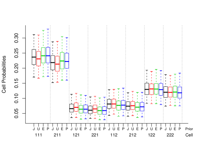
Figure 2: Antitoxin data: Boxplots summarizing 2.5%, 97.5% posterior percentiles and quantiles of the joint probabilities $\pi_{ABC}(i,j,k)$ for the MAP model (SC+A) for all prior set-ups (J=Jeffreys’, U=Unit Expected Cell, E=Empirical Bayes, P=Perks’) .

Similarly in Figure 3 we present boxplots providing posterior summaries for models $SC+A$, $AS+SC$ and $ASC$ under the UIP-Perks’ prior set-up. The first two models are the ones with highest posterior probabilities and all of their summaries have been calculated using Monte Carlo simulation (1000 values). The saturated was used mainly as reference model since it is the only one for which the posterior distributions are available analytically. From the figure we observe that the posterior distributions on the joint probabilities $\pi$ of the full table are quite different highly depending on the assumed model structure.

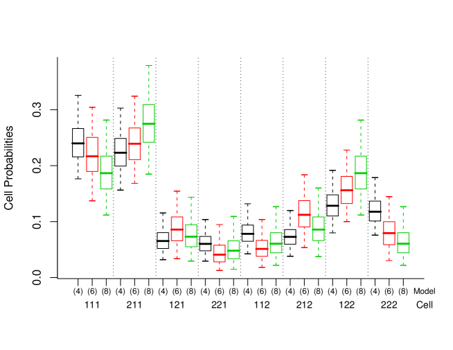
Figure 3: Antitoxin data: Boxplots summarizing 2.5%, 97.5% posterior percentiles and quantiles of the joint probabilities $\pi_{ABC}(i,j,k)$ for models SC+A, AS+SC and ASC (4, 6 and 8 respectively) under the UIP-Perks’ prior set-up.

Finally, posterior summaries for the probability parameters $\mbox{\boldmath$\pi$}^{G}$ and the marginal log-linear parameters $\mbox{\boldmath$\lambda$}^{G}$ for models $SC+A$, $AS+SC$ and $ASC$ (as described above) under the UIP-Perks’ prior are provided in Tables 4 and 5 respectively. All summaries of each element of $\mbox{\boldmath$\pi$}^{G}$ are obtained analytically based on the Beta distribution induced by the corresponding Dirichlet posterior distributions of $\mbox{\boldmath$\pi$}^{G}$. Posterior summaries of $\mbox{\boldmath$\lambda$}^{G}$ are estimated using the Monte Carlo strategy (1000 values) discussed in section 5. As commented in this section, some elements of $\mbox{\boldmath$\lambda$}^{G}$ for graphs $SC+A$ and $AS+SC$ are constrained to zero due the way we have constructed our model. Hence for $SC+A$, the maximal interaction terms for the disconnected sets $AS$, $AC$ and $ASC$, i.e. parameters $\lambda_{AS}(2,2)$, $\lambda_{AC}(2,2)$ and $\lambda_{ASC}(2,2,2)$, are constrained to be zero for all generated observations. Similar is the picture for model $AS+SC$, but now only marginals $AC$ and $ABC$ correspond to disconnected sets implying that $\lambda_{AC}(2,2)=\lambda_{ASC}(2,2,2)=0$.

Table 4: Posterior summaries of model parameters for models $SC+A$, $AS+SC$ and $ASC$ in Antitoxin data under the UIP-Perks’ prior set-up; $\widetilde{a}$ and $\widetilde{b}$ are the parameters of the resulted Beta marginal posterior distribution.

Model 4: $SC+A$					Beta Posterior
					Parameters
Parameter	Mean	St.dev.	$Q_{0.025}$	$Q_{0.975}$	$\widetilde{a}$	$\widetilde{b}$
$\pi_{SC}(1,1)$	0.47	0.055	0.36	0.57	37.25	42.75
$\pi_{SC}(2,1)$	0.13	0.037	0.06	0.21	10.25	69.75
$\pi_{SC}(1,2)$	0.15	0.040	0.08	0.24	12.25	67.75
$\pi_{A}(1)$	0.52	0.056	0.41	0.63	41.50	38.50
Model 6: $AS+SC$
Parameter	Mean	St.dev.	$Q_{0.025}$	$Q_{0.975}$	$\widetilde{a}$	$\widetilde{b}$
$\pi_{S|AC}(1|1,1)$	0.71	0.096	0.51	0.88	15.12	6.12
$\pi_{S|AC}(1|2,1)$	0.84	0.070	0.68	0.95	22.12	4.12
$\pi_{S|AC}(1|1,2)$	0.25	0.094	0.09	0.46	5.12	15.12
$\pi_{S|AC}(1|2,2)$	0.58	0.136	0.31	0.83	7.12	5.12
$\pi_{A}(1)$	0.52	0.056	0.41	0.63	41.50	38.50
$\pi_{C}(1)$	0.59	0.055	0.48	0.70	47.50	32.50
Model 8: $ASC$ (Saturated)
Parameter	Mean	St.dev.	$Q_{0.025}$	$Q_{0.975}$	$\widetilde{a}$	$\widetilde{b}$
$\pi(1,1,1)$	0.19	0.044	0.11	0.28	15.12	64.88
$\pi(2,1,1)$	0.28	0.050	0.18	0.38	22.12	57.88
$\pi(1,2,1)$	0.08	0.030	0.03	0.14	6.12	73.88
$\pi(2,2,1)$	0.05	0.025	0.01	0.11	4.12	75.88
$\pi(1,1,2)$	0.06	0.027	0.02	0.13	5.12	74.88
$\pi(2,1,2)$	0.09	0.032	0.04	0.16	7.12	72.88
$\pi(1,2,2)$	0.19	0.044	0.11	0.28	15.12	64.88
$\pi(2,2,2)$	0.06	0.027	0.02	0.13	5.12	74.88

Table 5: Antitoxin data: Posterior summaries for lambda for models SC+A, AS+SC and ASC under the UIP-Perks’ prior set-up

Model 4: $SC+A$
Parameter	Marginal table	Mean	St.dev.	$Q_{0.025}$	$Q_{0.975}$
$\lambda_{\emptyset}$	$M_{AS}$	-1.429	0.032	-1.513	-1.388
$\lambda_{A}(2)$	$M_{AS}$	-0.040	0.113	-0.258	0.181
$\lambda_{S}(2)$	$M_{AS}$	-0.245	0.118	-0.480	-0.021
$\lambda_{AS}(2,2)$	$M_{AS}$	0.000	0.000	0.000	0.000
$\lambda_{C}(2)$	$M_{AC}$	-0.194	0.116	-0.426	0.027
$\lambda_{AC}(2,2)$	$M_{AC}$	0.000	0.000	0.000	0.000
$\lambda_{SC}(2,2)$	$M_{ASC}$	0.460	0.134	0.199	0.735
$\lambda_{ASC}(2,2,2)$	$M_{ASC}$	0.000	0.000	0.000	0.000
Model 6: $AS+SC$
Parameter	Marginal table	Mean	St.dev.	$Q_{0.025}$	$Q_{0.975}$
$\lambda_{\emptyset}$	$M_{AC}$	-1.418	0.025	-1.483	-1.388
$\lambda_{A}(2)$	$M_{AC}$	-0.042	0.114	-0.261	0.173
$\lambda_{C}(2)$	$M_{AC}$	-0.195	0.110	-0.414	0.020
$\lambda_{AC}(2,2)$	$M_{AC}$	0.000	0.000	0.000	0.000
$\lambda_{S}(2)$	$M_{ASC}$	-0.238	0.137	-0.493	0.044
$\lambda_{AS}(2,2)$	$M_{ASC}$	-0.291	0.137	-0.554	-0.019
$\lambda_{SC}(2,2)$	$M_{ASC}$	0.437	0.137	0.178	0.712
$\lambda_{ASC}(2,2,2)$	$M_{ASC}$	-0.086	0.143	-0.370	0.207
Model 8: $ASC$ (Saturated)
Parameter	Marginal table	Mean	St.dev.	$Q_{0.025}$	$Q_{0.975}$
$\lambda_{\emptyset}$	$M_{ASC}$	-2.325	0.079	-2.504	-2.191
$\lambda_{A}(2)$	$M_{ASC}$	-0.106	0.134	-0.379	0.152
$\lambda_{S}(2)$	$M_{ASC}$	-0.246	0.131	-0.510	0.004
$\lambda_{AS}(2,2)$	$M_{ASC}$	-0.292	0.139	-0.576	-0.033
$\lambda_{C}(2)$	$M_{ASC}$	-0.136	0.143	-0.402	0.151
$\lambda_{AC}(2,2)$	$M_{ASC}$	-0.084	0.139	-0.355	0.202
$\lambda_{SC}(2,2)$	$M_{ASC}$	0.450	0.135	0.207	0.705
$\lambda_{ASC}(2,2,2)$	$M_{ASC}$	-0.074	0.143	-0.368	0.209

6.2 A $3\times 2\times 4$ table: Alcohol Data

We now examine a well known data set presented by Knuiman and Speed (1988) regarding a small study held in Western Australia on the relationship between Alcohol intake (A), Obesity (O) and High blood pressure (H); see Table 6.

Table 6: Alcohol Data

		Alcohol intake
		(drinks/days)
Obesity	High BP		0	1-2	3-5	6+
Low	Yes		5	9	8	10
	No		40	36	33	24
Average	Yes		6	9	11	14
	No		33	23	35	30
High	Yes		9	12	19	19
	No		24	25	28	29

In Table 7 we report posterior model probabilities and corresponding Log-marginal likelihoods for each models. Under all prior set-ups the posterior model probability is concentrated on models H+A+O, HA+O and HO+A. Empirical Bayes and UIP-Perks’ support the independence model (with posterior model probability of $0.878$ and $0.807$ respectively) whereas Jeffreys’ and Unit Expected support a more complex structure, HO+A (with posterior model probability of $0.837$ and $0.859$ respectively).

Table 7: Alcohol data: Posterior model probabilities and the corresponding Log marginal likelihoods; empty cell in posterior probabilities means that it is lower than $0.0001$

Posterior model probabilities ($\%$)
	Model
	H+A+O	HA+O	HO+A	AO+H	HA+HO	HA+AO	HO+AO	HAO
Prior Distribution	(1)	(2)	(3)	(4)	(5)	(6)	(7)	(8)
Jeffreys’	11.56	4.76	83.68
Unit Expected Cell	6.91	7.21	85.88
Empirical Bayes	87.81	0.07	12.12
Perks’	80.67	0.15	19.18
Log-marginal likelihood for each model
	Model
	H+A+O	HA+O	HO+A	AO+H	HA+HO	HA+AO	HO+AO	HAO
Prior Distribution	(1)	(2)	(3)	(4)	(5)	(6)	(7)	(8)
Jeffreys ($\alpha(i)=1/2$)	-79.22	-80.11	-77.24	-87.73	-90.44	-100.93	-98.06	-98.95
UEC ($\alpha(i)=1$)	-78.51	-78.47	-75.99	-84.70	-85.27	-93.99	-91.51	-91.46
Emprirical Bayes ($\alpha(i)=p(i)$)	-86.96	-94.10	-88.94	-107.26	-124.75	-143.06	-137.91	-145.04
Perks ($a(i)=1/|I|$)	-86.90	-93.19	-88.33	-107.10	-121.13	-139.89	-135.03	-141.33

To save space we do not report here posterior summaries for model parameters, they can be found in a separate appendix on the web page:

http://stat-athens.aueb.gr/~jbn/papers/paper21.htm.

7 Discussion and Final Comments

In this paper we have dealt with the Bayesian analysis of graphical models of marginal association for three way contingency tables. We have worked using the probability parameters of marginal tables required to fully specify each model. The proposed parametrization and the corresponding decomposition of the likelihood simplifies the problem and automatically imposes the marginal independences represented by the considered graph. By this way, the posterior model probabilities and the posterior distributions for the used parameters can be calculated analytically. Moreover, the posterior distributions of the marginal log-linear parameters $\mbox{\boldmath$\lambda$}^{G}$ and the probabilities $\pi$ of the full table can be easily obtained using simple Monte Carlo schemes. This approach avoids the problem of the inverse calculation of $\pi$ when the marginal association log-linear parameters $\lambda$ are available which can be only achieved via an iterative procedure; see Rudas and Bergsma (2004) and Lupparelli (2006) for more details.

An obvious extension of this work is to implement the same approach in tables of higher dimension starting from four way tables. Although most of the models in a four way contingency table can be factorized and analyzed in a similar manner, two type of graphs (the 4-chain and the cordless four-cycle graphs) cannot be decomposed in the above way. These models are not Markov equivalent to any directed acyclic graph (DAG). In fact each bidirected graph (which corresponds to a marginal association model) is equivalent to a DAG, i.e. a conditional association model, with the same set of variables if and only if it does not contain any 4-chain, see Pearl and Wermuth (1994). We believe that also in higher dimensional problems our approach can be applied to bidirected graphs that admit a DAG representation. For the graph that do not factorize, more sophisticated techniques must be adopted in order to obtain the posterior distribution of interest and the corresponding marginal likelihood needed for the model comparison (work in progress by the authors).

Another interesting subject is how to obtain the posterior distributions in the case that someone prefers to work directly with marginal log-linear parameters $\mbox{\boldmath$\lambda$}^{G}$ defined by (5). Using our approach, we impose a prior distribution on the probability parameters $\mbox{\boldmath$\pi$}^{G}$. The prior of $\mbox{\boldmath$\lambda$}^{G}$ cannot be calculated analytically since we cannot have the inverse expression of (5) in closed form. Nevertheless, we can obtain a sample from the imposed prior on $\mbox{\boldmath$\lambda$}^{G}$ using a simple Monte Carlo scheme. More specifically, we can generate random values of $\mbox{\boldmath$\pi$}^{G}$ from the Dirichlet based prior set-ups described in this paper. We calculate the joint probability vector $\pi$ according to the factorization of the graph under consideration and finally use (5) to obtain a sample from the imposed prior $f(\mbox{\boldmath$\lambda$}^{G}|G)$. This will give us an idea of the prior imposed on the log-linear parameters.

If prior information is expressed directly in terms of the log-linear parameters, see e.g Knuiman and Speed (1988) and Dellaportas and Forster (1999), the prior and the corresponding posterior distribution of $\mbox{\boldmath$\pi$}^{G}$ can be obtained using two alternative strategies.

One possibility is to approximate the distribution imposed on the elements of $\mbox{\boldmath$\pi$}^{G}$ via Dirichlet distributions with the parameters obtained in the following way. Firstly we generate random values from the prior imposed on the standard log-linear parameters for models of conditional association. For each set of generated values, we calculate the corresponding probabilities $\pi$ for the full table. Finally we obtain a sample for $\mbox{\boldmath$\pi$}^{G}$ via marginalization from each set of generated probabilities $\pi$. For every element of $\mbox{\boldmath$\pi$}^{G}$, we use the corresponding generated values to approximate the imposed prior by a Dirichlet distribution with the parameters estimated using the moment-matching approach. Note that this approach can only provide us a rough picture of the correct posterior distribution since the priors are only matched in terms of the mean and the variance while their shape can be totally different due to the properties of the Dirichlet distribution.

Similar will be the approach if the prior distributions $f(\mbox{\boldmath$\lambda$}^{G}|G)$ for the marginal log-linear parameters $\mbox{\boldmath$\lambda$}^{G}$ are available. The only problem here, in comparison to the simpler approach described in the previous paragraph, is the calculation of $\pi$ from each $\mbox{\boldmath$\lambda$}^{G}$. In order to achieve that we need to use iterative procedures; see Rudas and Bergsma (2004) and Lupparelli (2006).

A second approach is to directly calculate the prior distribution imposed on the probability parameters $\mbox{\boldmath$\pi$}^{G}$ starting from the prior $f(\mbox{\boldmath$\lambda$}^{G}|G)$ using equation (5). Note that the probabilities $\pi$ of the full table involved in (5) are simply a function of $\mbox{\boldmath$\pi$}^{G}$ depending on the structure $G$. Hence, the prior on $\pi$ will be given by

$$f(\mbox{\boldmath$\pi$}^{G}|G)=f(\mbox{\boldmath$\lambda$}^{G}|G)\left|\frac{\partial\mbox{\boldmath$\lambda$}^{G}}{\partial\mbox{\boldmath$p$}^{G}}\right|$$

where $\mbox{\boldmath$p$}^{G}$ is $\mbox{vec}(\mbox{\boldmath$\pi$}^{G})$ after removing the last element of each set of probability parameters and $\mbox{vec}(\mbox{\boldmath$\pi$}^{G})$ refers to $\mbox{\boldmath$\pi$}^{G}$ arranged in a vector form. The elements of the Jacobian are given by

$$\frac{\partial\lambda^{G}_{k}}{\partial p_{l}^{G}}=\sum_{i=1}^{col(\mbox{\footnotesize\bf C})}\left\{C_{ki}\left(\sum_{j=1}^{|{\cal I}|}M_{ij}\mbox{vec}({\mbox{\boldmath$\pi$}})_{j}\right)^{-1}\sum_{j=1}^{|{\cal I}|}M_{ij}\frac{\partial\mbox{vec}({\mbox{\boldmath$\pi$}})_{j}}{\partial p_{l}^{G}}\right\}$$

where $col(\mbox{\footnotesize\bf C})$ is the number of columns of $C$ matrix. For the saturated model the above equation simplifies to

$$\frac{\partial\lambda^{G}_{k}}{\partial p_{l}}=\sum_{i=1}^{col(\mbox{\footnotesize\bf C})}\frac{C_{ki}(M_{il}-M_{i|{\cal I}|})}{\sum_{j=1}^{|{\cal I}|}M_{ij}\mbox{vec}({\mbox{\boldmath$\pi$}})_{j}}$$

since $\mbox{vec}(\mbox{\boldmath$\pi$})_{j}=p_{j}^{G}$ for $j<|{\cal I}|$ and $\mbox{vec}(\mbox{\boldmath$\pi$})_{|{\cal I}|}=1-\sum_{j=1}^{|{\cal I}|-1}p_{j}^{G}$. After calculating the corresponding prior distribution $f(\mbox{\boldmath$\pi$}^{G}|G)$, we can work directly on $\mbox{\boldmath$\pi$}^{G}$ using an MCMC algorithm to generate values from the resulted posterior. A sample of $\mbox{\boldmath$\lambda$}^{G}$ can be again obtained in a direct way using (5). When no strong prior information is available, an independence Metropolis algorithm can be applied using as a proposal the Dirichlet distributions resulted from the likelihood part. Otherwise more sophisticated techniques might be needed. The authors are also exploring the possibility to extend the current work in this direction.

Appendix

1. Construction of Matrix $\mathbf{M}$

   Let ${\cal M}=\{M_{1},M_{2},\dots,M_{|{\cal M}|}\}$ be the set of considered marginals. Let ${\mathbf{B}}$ be a binary matrix of dimension $|\cal M|\times|{\cal V}|$ with elements $B_{iv}$ indicating whether a variable $v$ belongs to a specific marginal ${M}_{i}$. The rows of ${\mathbf{B}}$ correspond to the marginals in ${\cal M}$ whereas the columns to the variables. The variables follow a reverse ordering, that is column 1 corresponds to variable $X_{|\cal V|}$, column 2 to variable $X_{|{\cal V}|-1}$ and so on. Matrix $\mathbf{B}$ has elements

   $$B_{iv}=\left\{\begin{array}[]{rl}1&\mbox{ if $v\in{M}_{i}$ }\\ 0&\mbox{ otherwise.}\end{array}\right.,$$

   for every $v\in\cal V$.

   The marginalization matrix $\mathbf{M}$ can be constructed using the following rules.

   1. For each marginal ${M}_{i}$, the probability vector of the corresponding marginal table is given by $\mathbf{M}_{i}\mathbf{\pi}$; where $\mathbf{M}_{i}$ is calculated as a Kronecker product of matrices ${\mathbf{A}}_{iv}$

      $$\mathbf{M}_{i}=\bigotimes_{v\in{\cal V}}{\mathbf{A}}_{iv}$$

      with

      $$\mathbf{\mathbf{A}}_{iv}=\left\{\begin{array}[]{rl}{\mathbf{I}}_{\ell_{v}}&\mbox{ if }\;\;B_{iv}=1\\ {\mathbf{1}}_{\ell_{v}}^{T}&\mbox{ if }\;\;B_{iv}=0\end{array}\right.$$

      where $\ell_{v}$ is the number of levels for $v$ variable, ${\mathbf{I}}_{\ell_{v}}$ is the identity matrix of dimension $\ell_{v}\times\ell_{v}$ and ${\mathbf{1}}_{\ell_{v}}$ is a vector of dimension $\ell_{v}\times 1$ with all elements equal to one.

   2. Matrix $\mathbf{M}$ is constructed by stacking all the $\mathbf{M}_{i}$ matrices

      $$\mathbf{M}=\left(\begin{array}[]{l}\mathbf{M}_{1}\\ \vdots\\ \mathbf{M}_{i}\\ \vdots\\ \mathbf{M}_{|\mathbb{{M}}|}\end{array}\right)$$

2. Construction of Matrix $\mathbf{C}$

   Firstly we need to construct the design matrix $X$ for the saturated model corresponding to sum to zero constraints. It has has dimension $\left(\prod\limits_{v}\ \ell_{v}\right)\times\left(\prod\limits_{v}\ \ell_{v}\right)$ and can be obtained as

   $$\mathbf{X}=\underset{v\in{\cal V}^{R}}{\bigotimes}{\mathbf{J}}_{\ell_{v}}$$

   with

   $${\mathbf{J}}_{\ell_{v}}(r,c)=\left\{\begin{array}[]{rl}~{}1&\mbox{ if $c=1$ or $r=c$}\\ -1&\mbox{ if $r=1$ and $c>1$}\\ ~{}0&\mbox{ otherwise.}\end{array}\right.$$

   In matrix notation

   $${\mathbf{J}}_{\ell_{v}}=\left(\begin{array}[]{ll}1&-\mathbf{1}^{T}_{(\ell_{v}-1)}\\ \mathbf{1}_{(\ell_{v}-1)}&\mathbf{I}_{(\ell_{v}-1)\times(\ell_{v}-1)}\end{array}\right)$$

   where $\mathbf{1}_{(\ell_{v}-1)}$ is $({\ell_{v}-1})\times 1$ vector of ones while $\mathbf{I}_{({\ell_{v}-1})\times({\ell_{v}-1})}$ is an identity matrix of dimension $({\ell_{v}-1})\times({\ell_{v}-1})$.

   The contrast matrix $\mathbf{C}$ can be constructed by using the following rules.

   1. For each margin ${M}_{i}$ construct the design matrix $X_{i}$ corresponding to the saturated model (using sum to zero constraints) and invert it to get the contrast matrix for the saturated model $\mathbf{C}_{i}=X^{-1}$ . Let $\mathbf{C}_{i}^{*}$ be a submatrix of $\mathbf{C}_{i}$ obtained by deleting rows not corresponding to elements of $\mbox{\boldmath$\cal E$}_{M_{i}}$ (the effects that we wish to estimate from margin ${M}_{i}$) .

   2. The contrast matrix $\mathbf{C}$ is obtained by direct sum of the $C_{i}^{*}$ matrices as follow

      $$\mathbf{C}=\bigoplus_{i:~{}{\cal M}_{i}\in{\mathbb{M}}}\mathbf{C}_{i}^{*}$$

      that is it is a block diagonal matrix with $(\mathbf{C}_{1}^{*};{M}_{i}\in{\cal M})$ as the blocks. For example $C_{i}^{*}\bigotimes C_{2}=\bigoplus_{i=1}^{2}C^{*}_{i}$ is the block diagonal matrix with $C_{1}$ and $C_{2}$ as blocks.

References

- [1]
- [2] Bartlett, M. S. (1957). A comment on Lindley’s statistical paradox. Biometrika, 44, 533-534.
- [3]
- [4] Bergsma, W. P. and Rudas, T. (2002). Marginal log-linear models for categorical data. Annals of Statistics, 30, 140-159.
- [5]
- [6] Chen, M.H., Ibrahimb, J.G. and Shao, Q. M. (2000). Power prior distributions for generalized linear models. Journal of Statistical Planning and Inference, 84, 121-137.
- [7]
- [8] Cox, D. R. and Wermuth, N. (1993). Linear dependencies represented by chain graphs (with discussion). Statistical Science, 8, 204-218, 247-277.
- [9]
- [10] Dawid A.P. and Lauritzen S.L. (1993). Hyper-Markov laws in the statistical analysis of decomposable graphical models, Annals of Statistics, 21, 1272-1317.
- [11]
-
[12]
Dawid, A.P. and Lauritzen, S.L. (2000). Compatible
prior distributions. In Bayesian Methods with Applications
to Science Policy and Official Statistics. The sixth world meeting
of the International Society for Bayesian Analysis (ed. E.I.
George), 109-118.
http://www.stat.cmu.edu/ISBA/index.html. - [13]
- [14] Dellaportas, P., Forster, J.J. and Ntzoufras I. (2002). On Bayesian model and variable selection using MCMC. Statistics and Computing, 12, 27-36.
- [15]
- [16] Drton, M. and Richardson, T. S. (2008). Binary models for marginal independence. Journal of the Royal Statistical Society, Ser. B , 70, 287-309.
- [17]
- [18] Glonek, G. J. N. and McCullagh, P. (1995). Multivariate logistic models. Journal of the Royal Statistical Society, Ser. B, 57, 533-546.
- [19]
- [20] Healy, M.J.R. (1988). Glim: An Introduction, Claredon Press, Oxford, UK.
- [21]
- [22] Ibrahim J.G. and Chen M. H. (2000). Power Prior Distributions for Regression Models. Statistical Science, 15, 46- 60.
- [23]
- [24] Kauermann, G. (1996). On a dualization of graphical Gaussian models. Scandinavian Journal of Statistics, 23, 105 116.
- [25]
- [26] Knuiman, M. W. and Speed, T. P. (1988). Incorporating prior information into the analysis of contingency tables. Biometrics, 44 , 1061-1071.
- [27]
- [28] Lindley, D. V. (1957). A statistical paradox. Biometrika, 44, 187 192.
- [29]
- [30] Lupparelli, M. (2006). Graphical models of marginal independence for categorical variables. Ph. D. thesis, University of Florence.
- [31]
- [32] Lupparelli, M., Marchetti, G. M., Bersgma, W. P. (2008). Parameterization and fitting of bi-directed graph models to categorical data. arXiv:0801.1440v1
- [33]
- [34] Pearl, J. and Wermuth, N. (1994). When can association graphs admit a causal interpretation? In P. Cheesman and W. Oldford, eds., Models and data, artifical intelligence and statistics iv. Springer, New York, 205-214.
- [35]
- [36] Perks, W. (1947). Some observations on inverse probability including a new indifference rule. journal of the institute of actuaries 73, 285-334.
- [37]
- [38] Richardson, T. S. (2003). Markov property for acyclic directed mixed graphs. Scandinavian Journal of Statistics 30, 145-157.
- [39]
- [40] Roverato A. and Consonni G. (2004) Compatible Prior Distributions for DAG models. Journal of the Royal Statistical Society series B, 66, 47-61.
- [41]
- [42] Rudas, T. and Bergsma, W. P. (2004). On applications of marginal models for categorical data. Metron LXII, 1 25.
- [43]