Theory of Raman transitions in cavity QED

Abstract

We present two schemes for driving Raman transitions between the ground state hyperfine manifolds of a single atom trapped within a high-finesse optical cavity. In both schemes, the Raman coupling is generated by standing-wave fields inside the cavity, thus circumventing the optical access limitations that free-space Raman schemes must face in a cavity system. These cavity-based Raman schemes can be used to coherently manipulate both the internal and the motional degrees of freedom of the atom, and thus provide powerful tools for studying cavity quantum electrodynamics. We give a detailed theoretical analysis of each scheme, both for a three-level atom and for a multi-level cesium atom. In addition, we show how these Raman schemes can be used to cool the axial motion of the atom to the quantum ground state, and we perform computer simulations of the cooling process.

I Introduction

Systems consisting of a single atom coupled to a high-finesse optical cavity are of fundamental importance to quantum optics and quantum information science. Such cavity QED systems have been experimentally implemented using neutral atoms ye99 ; mckeever03a ; maunz04 ; sauer04 ; nussmann05a ; miller05 and ions guth01 ; mundt02 , and have been the subject of numerous theoretical studies englert91 ; haroche91 ; holland91 ; herkommer92 ; storey92 ; ren95 ; herkommer96 ; scully96 . In particular, such systems play a key role in proposals for scalable quantum computation pellizzari95 ; duan04 and distributed quantum networks cirac97 ; briegel00 . An important requirement for many of these proposals is the ability to coherently control the internal and motional degrees of freedom of the trapped atom, and Raman transitions provide the means for meeting this requirement.

Raman transitions are powerful tools that have diverse applications in atomic physics, including spectroscopy dotesenko04 , precision measurement clade06 ; gustavson97 , and coherent state manipulation wineland03 , and have been used to coherently control the motional degrees of freedom of trapped ions monroe95 ; leibfried03 and of neutral atoms trapped in optical lattices hamann98 ; perrin98 ; vuletic98 . Until recently, however, Raman transitions had not been incorporated into cavity QED. The practical challenge of implementing a free-space Raman scheme in cavity QED lies in the presence of the cavity itself, which offers limited optical access to the atom within, especially in the strong coupling regime miller05 . As first proposed in boozer05 , these optical access limitations can be circumvented by implementing a cavity-based Raman scheme, in which the Raman coupling is generated by standing-wave fields inside the cavity.

In this paper, we provide the theoretical background behind two such cavity-based schemes for driving Raman transitions between the hyperfine ground state manifolds of a single atom optically trapped within a high-finesse cavity. Both schemes have been recently implemented and validated experimentally, and have been used to extend the trapping lifetime of a near-resonantly driven atom boca04 , to cool the axial motion of an atom to the quantum ground state of its trapping potential boozer06 , and to optically pump an atom into a specific Zeeman state boozer07 .

The paper is organized as follows. In section II, we describe how a single atom is trapped inside the cavity by means of an optical dipole trap. In section III, we present the two schemes for driving Raman transitions in the trapped atom. We treat the atom using a three-level model, and show that the internal and motional degrees of freedom of the atom can be described using an effective Hamiltonian that has the same form for both schemes. In section IV, we quantize the axial motion of the atom, and show how the Raman couplings allow one to drive transitions that change the vibrational quantum number for motion along the cavity axis. We present both analytic results, which apply to atoms that are sufficiently cold, and numerical results, which apply to atoms of arbitrary temperature. In section V, we describe how the Raman couplings are modified when we take into account the multiplicity of levels in a physically realistic cesium atom. We show that the Raman schemes drive transitions between individual Zeeman states in the two hyperfine ground state manifolds, and we derive the Rabi frequencies for these Zeeman transitions. Finally, in section VI, we show how Raman transitions can be used to cool the axial motion of the atom to the quantum ground state, and we present computer simulations of the cooling process.

II Trapping an atom inside the cavity

The optical cavity we will be considering consists of two symmetric mirrors separated by a distance $L$ (details of the cavity are given in Appendix A). An atom is trapped inside the cavity by means of a far off-resonance trap (FORT), which is created by driving one of the cavity modes with light that is red-detuned from a dipole transition in the atom. The red-detuned light forms a standing wave inside the cavity, and the coupling of the atom to the light causes it to be attracted to the points of maximum intensity in the standing wave.

The operation of the FORT can be understood by considering a simple two-level model in which the atom has a single ground state $g$ and a single excited state $e$. Let $\omega_{e}$ denote the frequency of the $g-e$ transition, and let $\omega_{F}$ denote the frequency of the FORT light. We will assume that the FORT resonantly drives mode $n_{F}$ of the cavity, so $\omega_{F}=2\pi\nu_{FSR}\,n_{F}$, where $\nu_{FSR}=1/2L$ is the free spectral range. The Hamiltonian for the system is

$$H=\omega_{e}|e\rangle\langle e|+(\hat{\Omega}+\hat{\Omega}^{\dagger})\,\cos\omega_{F}t,$$ (1)

where

$$\hat{\Omega}\equiv\Omega_{F}\,\psi_{F}(\vec{r})\,|g\rangle\langle e|.$$ (2)

Here $\vec{r}$ is the position of the atom, $\psi_{F}(\vec{r})$ is a dimensionless quantity that characterizes the shape of the cavity mode (see Appendix A), and $\Omega_{F}$ is the Rabi frequency of the light at a point of maximum intensity. We can simplify this Hamiltonian by making the rotating wave approximation and then performing a unitary transformation to eliminate the time dependence:

$$H=-\Delta_{F}|e\rangle\langle e|+\frac{1}{2}(\hat{\Omega}+\hat{\Omega}^{\dagger}),$$ (3)

where $\Delta_{F}\equiv\omega_{L}-\omega_{e}$ is the detuning of the FORT from the atom (note that because the FORT is red-detuned, $\Delta_{F}<0$). In the limit that the FORT is far-detuned ($|\Delta_{F}|\gg\Omega_{F}$), we can adiabatically eliminate the excited state (see boozer05 ) to obtain an effective Hamiltonian for the ground state:

$$H_{E}=\frac{1}{4\Delta_{F}}\hat{\Omega}\hat{\Omega}^{\dagger}=U(\vec{r})\,|g\rangle\langle g|,$$ (4)

where

$$U(\vec{r})\equiv-U_{F}\,|\psi_{F}(\vec{r})|^{2}$$ (5)

describes a trapping potential with depth $U_{F}\equiv\Omega_{F}^{2}/4|\Delta_{F}|$. For the experiments described in boca04 ; boozer06 ; boozer07 , the power in the FORT beam is set such that $U_{F}\simeq(2\pi)(50\,\mathrm{MHz})$. To describe the shape of the potential, it is convenient to use a cylindrical coordinate system centered on the cavity axis: we will let $z$ and $\rho$ denote the axial and radial coordinates of the atom, where the cavity mirrors are located at $z=0$ and $z=L$. Using equation (98) to substitute for the mode shape $\psi_{F}(\vec{r})$ in this coordinate system, we find that

$$U(\vec{r})=-U_{F}\,e^{-2\rho^{2}/w_{F}^{2}}\,\sin^{2}k_{F}z,$$ (6)

where $k_{F}\equiv\pi n_{F}/L$ is the wavenumber for the FORT mode $n_{F}$. The minima of the potential occur at the points $\rho=0$, $z=z_{r}$, where $z_{r}$ is defined such that

$$k_{F}z_{r}=\pi(r+1/2).$$ (7)

Since $0<z_{r}<L$, we find that $r=1,...,n_{F}-1$; thus, there are $n_{F}$ distinct FORT wells in which an atom can be trapped. Let us assume that the atom is trapped in FORT well $r$. It is convenient to define a coordinate $x=z-z_{r}$ that gives the axial displacement of the atom from the potential minimum of this well. We can then express the trapping potential as

$$U(\vec{r})=-U_{F}\,e^{-2\rho^{2}/w_{F}^{2}}\,\cos^{2}k_{F}x.$$ (8)

Near the bottom of the well the potential can be approximated as harmonic,

$$U(\vec{r})\simeq-U_{F}+\frac{1}{2}m\omega_{r}^{2}\rho^{2}+\frac{1}{2}m\omega_{a}^{2}x^{2},$$ (9)

where $\omega_{r}$ and $\omega_{a}$, the radial and axial vibrational frequencies, are given by

$$\frac{1}{2}m\omega_{r}^{2}=2U_{F}/w_{F}^{2},\qquad\frac{1}{2}m\omega_{a}^{2}=U_{F}k_{F}^{2}.$$ (10)

The corresponding periods $2\pi/\omega_{r}$ and $2\pi/\omega_{a}$ characterize the timescales for radial and axial motion. For the experiments described in boca04 ; boozer06 ; boozer07 , the vibrational frequencies are $\omega_{r}\simeq(2\pi)(5\,\mathrm{kHz})$ and $\omega_{a}\simeq(2\pi)(500\,\mathrm{kHz})$, so the timescale for radial motion is much longer than the timescale for axial motion. We will be interested in describing the evolution of system over timescales that are short compared to the timescale for radial motion, but not necessarily short compared to the timescale for axial motion. For such timescales we can view the atom as being radially stationary, and take $\rho$ to be a constant parameter that enters into the potential for the axial motion. Thus, dropping a constant term, we can express the potential for the axial motion as

$$U(\vec{r})=U_{\rho}\sin^{2}k_{F}x,$$ (11)

where $U_{\rho}\equiv U_{F}\,e^{-2\rho^{2}/w_{F}^{2}}$ is the axial trap depth at radial coordinate $\rho$.

III Raman coupling for a three-level model

III.1 Effective Hamiltonian

To show how a Raman coupling can be generated in a trapped atom, let us now consider a three-level model in which the atom has two ground states $a$ and $b$, which correspond to the ground state hyperfine manifolds of a multi-level atom, and a single excited state $e$. The excited state has energy $\omega_{e}$, and the ground states $a$ and $b$ have energies $-\Delta_{HF}/2$ and $+\Delta_{HF}/2$, where $\Delta_{HF}$ is the ground state hyperfine splitting. The Hamiltonian for the atom is

$$H_{0}=\omega_{e}|e\rangle\langle e|+\frac{1}{2}\Delta_{HF}\sigma_{z},$$ (12)

where

$$\sigma_{z}\equiv|b\rangle\langle b|-|a\rangle\langle a|.$$ (13)

We can generate a Raman coupling between the two ground states by driving one of the cavity modes with a pair of beams that are tuned into Raman resonance with the ground state hyperfine splitting of the atom. Let us denote the optical frequencies of these beams by $\omega_{\pm}=\omega_{L}\pm\delta_{R}/2$, where $\omega_{L}$ is the average frequency and $\delta_{R}$ is the frequency difference (see Figure 1). Also, let us define a parameter $\delta=\delta_{R}-\Delta_{HF}$ that gives the Raman detuning of the beams; we will assume that the beams are tuned close to Raman resonance, so $|\delta|\ll\Delta_{HF}$. The beams generate standing-wave fields inside the cavity, and the coupling of the atom to these fields is described by the Hamiltonian

$$H_{R}=(\hat{\Omega}_{+}+\hat{\Omega}_{+}^{\dagger})\cos\omega_{+}t+(\hat{\Omega}_{-}+\hat{\Omega}_{-}^{\dagger})\cos\omega_{-}t,$$ (14)

where

$$\hat{\Omega}\pm\equiv\Omega_{\pm}\,\psi(\vec{r})\,A,$$ (15)

and

$$A\equiv(|a\rangle+|b\rangle)\langle e|$$ (16)

is an atomic lowering operator. Here $\vec{r}$ is the position of the atom, $\psi(\vec{r})$ is a dimensionless quantity that characterizes the shape of the driven mode (see Appendix A), and $\Omega_{\pm}$ are the Rabi frequencies of the fields at a point of maximum intensity. For simplicity, we have assumed that the $a-e$ and $b-e$ transitions couple to the light fields with equal strength.

The total Hamiltonian for the system is $H=H_{0}+H_{R}$. We can simplify this Hamiltonian by making the rotating wave approximation and then performing a unitary transformation:

$$H=-\Delta|e\rangle\langle e|+\frac{1}{2}\Delta_{HF}\sigma_{z}+\hat{B}+\hat{B}^{\dagger},$$ (17)

where

$$\hat{B}\equiv\frac{1}{2}(\hat{\Omega}_{+}\,e^{i\delta_{R}t/2}+\hat{\Omega}_{-}\,e^{-i\delta_{R}t/2}),$$ (18)

and $\Delta\equiv\omega_{L}-\omega_{e}$ describes the overall detuning of the optical fields from the excited state. We will assume that the fields are far-detuned from the atom ($|\Delta|\gg\Omega_{\pm}$), so we can further simplify the Hamiltonian by adiabatically eliminating the excited state to obtain an effective Hamiltonian for the ground states:

$$H_{E} = \frac{1}{2}\Delta_{HF}\sigma_{z}+\frac{1}{\Delta}\hat{B}\hat{B}^{\dagger},$$ (19)

$$= \frac{1}{2}\Delta_{HF}\sigma_{z}-V_{E}\,|\psi(\vec{r})|^{2}-V_{E}\,|\psi(\vec{r})|^{2}\,\sigma_{x}+\Omega_{E}\,|\psi(\vec{r})|^{2}\cos\delta_{R}t+\Omega_{E}\,|\psi(\vec{r})|^{2}\,\sigma_{x}\cos\delta_{R}t,$$ (20)

where

$$V_{E}\equiv(\Omega_{+}^{2}+\Omega_{-}^{2})/4|\Delta|,\qquad\Omega_{E}\equiv\Omega_{+}\,\Omega_{-}/2\Delta,$$ (21)

and

$$\sigma_{x}\equiv|a\rangle\langle b|+|b\rangle\langle a|.$$ (22)

We will assume that the optical fields are weak enough that $V_{E},\Omega_{E}\ll\Delta_{HF}$, so the first term of $H_{E}$ dominates and to a good approximation the eigenstates of $H_{E}$ are $|a\rangle$ and $|b\rangle$. The second term of $H_{E}$ describes a state-independent level shift, which is analogous to the FORT potential we derived in the previous section. The third term of $H_{E}$ gives a state-dependent correction to the level shift, which is of order $V_{E}^{2}/\Delta_{HF}$ and may therefore be neglected. The fourth term of $H_{E}$ describes a modulation of the state-independent level shift at frequency $\delta_{R}$. Because we have assumed that the system is tuned near to Raman resonance, $\delta_{R}$ is of the same order as the hyperfine splitting $\Delta_{HF}$. For cesium, the atom used in the experiments described in boca04 ; boozer06 ; boozer07 , the hyperfine splitting is $\Delta_{HF}=(2\pi)(9.2\,\mathrm{GHz})$, which is much larger than the harmonic frequencies $\omega_{r}$ and $\omega_{a}$ that characterize the timescales for atomic motion. Thus, over the motional timescales the fourth term of $H_{E}$ averages to zero and may also be neglected. After making these approximations, we are left with

$$H_{E}=\frac{1}{2}\Delta_{HF}\sigma_{z}-V_{E}\,|\psi(\vec{r})|^{2}+\Omega_{E}\,|\psi(\vec{r})|^{2}\sigma_{x}\cos\delta_{R}t.$$ (23)

We can further simplify the effective Hamiltonian by making the rotating wave approximation and then performing a unitary transformation to eliminate the time-dependence:

$$H_{E}=-\frac{\delta}{2}\sigma_{z}-V_{E}\,|\psi(\vec{r})|^{2}+\frac{1}{2}\,\Omega_{E}\,|\psi(\vec{r})|^{2}\,\sigma_{x}.$$ (24)

This Hamiltonian describes an effective two-level atom with ground state $a$ and excited state $b$, which is driven by a classical field with Rabi frequency $\Omega_{E}\,|\psi(\vec{r})|^{2}$ and detuning $\delta$. We will now use this effective Hamiltonian to describe two schemes for driving Raman transitions in a trapped atom.

Figure 1: Level diagram for the three-level atom. Shown are the ground states $a$ and $b$, the excited state $e$, and the pair of optical fields at frequencies $\omega_{+}$ and $\omega_{-}$.

III.2 FORT-Raman configuration

In the first scheme, which we will call the FORT-Raman configuration, the FORT itself forms one leg of a Raman pair. To form the other leg of the pair we add a much weaker beam, which we will call the Raman beam, that drives the same cavity mode as the FORT but is detuned from the cavity resonance by $\delta_{R}$. This configuration was first proposed in boozer05 , and formed the basis of the optical pumping scheme described in boozer07 and of the cooling scheme used in boca04 to extend the lifetime of a trapped atom. Let us denote the optical frequencies of the FORT and Raman beams by $\omega_{F}$ and $\omega_{R}=\omega_{F}+\delta_{R}$, and their maximum Rabi frequencies inside the cavity by $\Omega_{F}$ and $\Omega_{R}$. We can then apply the results of section III.1 to obtain an effective Hamiltonian $H_{E}$ that describes the FORT-Raman pair. We will assume that the Raman beam is blue-detuned from the FORT ($\delta_{R}>0$), so we take the $\Omega_{+}$ field to be the Raman field and the $\Omega_{-}$ field to be the FORT field; if the Raman beam is red-detuned from the FORT ($\delta_{R}<0$) then we reverse these identifications.

As was discussed in section II, we treat the atom as being radially stationary, and consider only the axial motion. Thus, the total Hamiltonian for the atom is given by

$$H=\frac{p^{2}}{2m}+H_{E}.$$ (25)

Here $p$ is the momentum of the atom in the axial direction, and $H_{E}$ is given by equation (24) with $\Omega_{E}=\Omega_{F}\Omega_{R}/2\Delta_{F}$ and $V_{E}=U_{F}+U_{R}$, where $U_{F}=\Omega_{F}^{2}/4|\Delta_{F}|$ and $U_{R}=\Omega_{R}^{2}/4|\Delta_{F}|$ are the maximum level shifts due to the FORT and Raman fields individually, and $\Delta_{F}=\omega_{F}-\omega_{e}$ is the overall detuning of the FORT and Raman beams from the atom. It is convenient to express $H$ as $H=H_{ext}+H_{int}$, where

$$H_{ext}=\frac{p^{2}}{2m}-V_{E}\,|\psi_{F}(\vec{r})|^{2}$$ (26)

describes the axial motion of the atom, and

$$H_{int}=-\frac{\delta}{2}\sigma_{z}+\frac{1}{2}\,\Omega_{E}\,|\psi_{F}(\vec{r})|^{2}\,\sigma_{x}$$ (27)

describes the internal state of the atom. Typically the powers of the FORT and Raman beams are such that $\Omega_{E}\simeq(2\pi)(200\,\mathrm{kHz})$ and $U_{F}\simeq(2\pi)(50\,\mathrm{MHz})$, and for these values $U_{R}/U_{F}\sim(\Omega_{E}/U_{F})^{2}\simeq 2\times 10^{-5}$. Thus, we can neglect the level shift of the Raman beams and approximate $H_{ext}$ as

$$H_{ext}=\frac{p^{2}}{2m}+U(\vec{r}),$$ (28)

where $U(\vec{r})=-U_{F}\,|\psi_{F}(\vec{r})|^{2}$ is the FORT trapping potential. As in section II, we will assume that the atom is trapped in FORT well $r$, and define a coordinate $x=z-z_{r}$ that gives the axial displacement of the atom from the well minimum. Note that

$$|\psi_{F}(\vec{r})|^{2}=e^{-2\rho^{2}/w_{F}^{2}}\,\sin^{2}k_{F}z=e^{-2\rho^{2}/w_{F}^{2}}\,\cos^{2}k_{F}x,$$ (29)

where we have substituted for the FORT mode shape $\psi_{F}(\vec{r})$ using equation (98) and for $k_{F}z_{r}$ using equation (7). Thus, we can express the internal Hamiltonian as

$$H_{int}=-\frac{\delta}{2}\sigma_{z}+\frac{1}{2}\,\Omega_{\rho}\cos^{2}k_{F}x\,\sigma_{x},$$ (30)

where $\Omega_{\rho}\equiv\Omega_{E}\,e^{-2\rho^{2}/w_{F}^{2}}$ is the effective Rabi frequency for an atom at radial coordinate $\rho$.

III.3 Raman-Raman configuration

For the second configuration, which we will call the Raman-Raman configuration, the FORT drives mode $n_{F}$ of the cavity at frequency $\omega_{F}$, and a pair of Raman beams drives mode $n_{R}$ of the cavity at frequency $\omega_{R}$. This configuration was used to perform the ground-state cooling described in boozer06 . We will assume that the Raman beams have equal powers and are tuned symmetrically about the cavity resonance, so the frequencies of these beams can be expressed as $\omega_{R}\pm\delta_{R}/2$. Let $\Omega_{F}$ denote the maximum Rabi frequency for the FORT beam, and let $\Omega_{R}$ denote the maximum Rabi frequency for one of the Raman beams. Using the results of section III.1, we can describe the coupling of the atom to the pair of Raman fields in terms of an effective Hamiltonian $H_{E}$.

As was discussed in section II, we treat the atom as being radially stationary, and consider only the axial motion. Thus, the total Hamiltonian for the system is

$$H=\frac{p^{2}}{2m}+U(\vec{r})+H_{E}.$$ (31)

The first term describes the kinetic energy of the atom due to axial motion, and the second term describes the FORT potential $U(\vec{r})=-U_{F}\,|\psi_{F}(\vec{r})|^{2}$, where $U_{F}=\Omega_{F}^{2}/4|\Delta_{F}|$ is the FORT depth. The third term is given by equation (24) with $V_{E}=2U_{R}$, $U_{R}=\Omega_{R}^{2}/4|\Delta_{R}|$, and $\Omega_{E}=\Omega_{R}^{2}/2\Delta_{R}$, where $\Delta_{R}\equiv\omega_{R}-\omega_{e}$ is the overall detuning of the Raman pair from the atom. It is convenient to express $H$ as $H=H_{ext}+H_{int}$, where

$$H_{ext}=\frac{p^{2}}{2m}+U(\vec{r})-V_{E}|\psi_{R}(\vec{r})|^{2}$$ (32)

describes the motion of the atom, and

$$H_{int}=-\frac{\delta}{2}\sigma_{z}+\frac{1}{2}\,\Omega_{E}\,|\psi_{R}(\vec{r})|^{2}\,\sigma_{x}$$ (33)

describes the internal state of the atom.

Note that because the FORT and Raman beams drive different cavity modes, the registration of the standing waves corresponding to the two beams depends on the axial position of the atom, and therefore on the particular FORT well in which the atom is trapped. This is in contrast to the FORT-Raman configuration, for which the FORT and Raman standing waves are always perfectly registered. One consequence of the well-dependence of the registration is that the level shift $V_{E}$ due to the Raman pair distorts different FORT wells in different ways. We calculate this effect in Appendix B, but for now we note that for the typical parameters $\Omega_{E}\simeq(2\pi)(200\,\mathrm{kHz})$, $U_{F}\simeq(2\pi)(50\,\mathrm{MHz})$ the ratio of the level shifts due to the FORT and Raman beams is $U_{R}/U_{F}=\Omega_{E}/U_{F}\simeq 4\times 10^{-3}$. Thus $V_{E}\ll U_{F}$, so we can neglect the $V_{E}$ term and approximate $H_{ext}$ as

$$H_{ext}=\frac{p^{2}}{2m}+U(\vec{r}).$$ (34)

As in section II, we will assume that the atom is trapped in FORT well $r$, and define a coordinate $x=z-z_{r}$ that gives the axial displacement of the atom from the well minimum. Note that

$$|\psi_{R}(\vec{r})|^{2}=e^{-2\rho^{2}/w_{R}^{2}}\,\sin^{2}k_{R}z=e^{-2\rho^{2}/w_{R}^{2}}\,\cos^{2}(k_{R}x+\alpha),$$ (35)

where $\alpha=(k_{R}-k_{F})z_{r}$ is the phase difference between the FORT and Raman beams at the bottom of FORT well $r$. Here we have substituted for the FORT mode shape $\psi_{F}(\vec{r})$ using equation (98) and for $k_{F}z_{r}$ using equation (7). We will assume that the FORT and Raman beams drive nearby modes of the cavity, so $|n_{R}-n_{F}|\ll n_{R},n_{F}$. In this limit $(k_{R}-k_{F})x\ll 1$ and $w_{R}\simeq w_{F}$, so we can approximate equation (35) as

$$|\psi_{R}(\vec{r})|^{2}=e^{-2\rho^{2}/w_{F}^{2}}\,\cos^{2}(k_{F}x+\alpha).$$ (36)

Thus, we can express the internal Hamiltonian as

$$H_{int}=-\frac{\delta}{2}\sigma_{z}+\frac{1}{2}\,\Omega_{\rho}\cos^{2}(k_{F}x+\alpha)\,\sigma_{x},$$ (37)

where $\Omega_{\rho}\equiv\Omega_{E}\,e^{-2\rho^{2}/w_{F}^{2}}$ is the effective Rabi frequency for an atom at radial coordinate $\rho$.

III.4 Summary of Raman schemes

We have shown that that for both the FORT-Raman and the Raman-Raman configurations the Hamiltonian has the form $H=H_{ext}+H_{int}$, where

$$H_{ext} = \frac{p^{2}}{2m}+U_{\rho}\,\sin^{2}k_{F}x,$$ (38)

$$H_{int} = -\frac{\delta}{2}\sigma_{z}+\frac{1}{2}\,\Omega_{\rho}\,\cos^{2}(k_{F}x+\alpha)\,\sigma_{x}.$$ (39)

For the FORT-Raman configuration $\alpha=0$, and for the Raman-Raman configuration $\alpha=(k_{R}-k_{F})z_{r}$ for an atom trapped in FORT well $r$. The Hamiltonian $H_{ext}$ describes the motion of the atom in the axial potential and is independent of the atomic state, and the Hamiltonian $H_{int}$ describes a Raman coupling between the ground states that depends on the axial position of the atom.

For either the FORT-Raman or the Raman-Raman configuration, the Raman coupling described by $H_{int}$ can be turned off by turning off one of the beams in the Raman pair (note that for FORT-Raman configuration the FORT beam must always be on in order to maintain the trapping potential, so for this configuration one must turn off the Raman beam). Alternatively, one can keep the beams in the Raman pair on at all times and turn off the Raman coupling by tuning the pair out of Raman resonance ($|\delta|\gg\Omega_{\rho}$). As we have seen, there is a small level shift due to the Raman beams, which we neglected when writing down the above expression for $H_{ext}$, and this detuning-based method has the advantage that these level shifts are always present regardless of whether the Raman coupling is on or off. With the first method, these level shifts cause a slight change in the trapping potential whenever the Raman coupling is turned on or off, which could potentially heat the atom or cause other problems.

IV Quantization of axial motion

For many applications, such as Raman sideband cooling, it is necessary to quantize the axial motion; that is, to treat the axial position $x$ and momentum $p$ as quantum operators. We first show how this is achieved for cold atoms, and then discuss some numerical results that apply to atoms of arbitrary temperature.

IV.1 Approximate form of the Hamiltonian for cold atoms

For cold atoms the axial trapping potential is nearly harmonic, where the harmonic frequency $\omega$ is given by

$$\omega=(2U_{\rho}/m)^{1/2}\,k_{F}=\omega_{a}\,e^{-\rho^{2}/w_{F}^{2}}.$$ (40)

We can quantize the axial motion by introducing phonon creation and annihilation operators operators $b^{\dagger}$ and $b$, which are related to $x$ and $p$ by

$$x=(2m\omega)^{-1/2}\,(b+b^{\dagger}),\qquad p=-i(m\omega/2)^{1/2}\,(b-b^{\dagger}).$$ (41)

From these relations, we find that

$$k_{F}x=\eta(b+b^{\dagger}),$$ (42)

where $\eta$, the Lamb-Dicke parameter, is given by $\eta\equiv(2m\omega)^{-1/2}\omega_{F}$. Note that because $\omega$ depends on the radial coordinate $\rho$, the Lamb-Dicke parameter also depends on $\rho$.

If the atoms are sufficiently cold, we can obtain a reasonable approximation to $H=H_{int}+H_{ext}$ by expanding in $\eta$ and retaining terms only up to second order; from equations (38), (39), and (42), we find that

$$H_{ext} = \omega(1/2+b^{\dagger}b)-\omega(\eta^{2}/12)(b+b^{\dagger})^{4},$$ (43)

$$H_{int} = -\frac{\delta}{2}\sigma_{z}+\frac{1}{2}\Omega_{\rho}\,((1/2)(1+\cos 2\alpha)-\eta(b+b^{\dagger})\sin 2\alpha-\eta^{2}(b+b^{\dagger})^{2}\cos 2\alpha)\,\sigma_{x}.$$ (44)

It is convenient to form a basis of states $\{|a,n\rangle,|b,n\rangle\}$ for the system by taking tensor products of the internal states $|a\rangle$ and $|b\rangle$ with the motional Fock states $\{|n\rangle\}$. To order $\eta^{2}$ these product states are eigenstates of $H_{ext}$, where pairs of states $|a,n\rangle$, $|b,n\rangle$ with the same vibrational quantum number $n$ are degenerate and have energy

$$E_{n}=\langle a,n|H_{ext}|a,n\rangle=\langle b,n|H_{ext}|b,n\rangle=\omega(1/2+n)-\omega(\eta^{2}/4)(1+2n+2n^{2}).$$ (45)

The Raman coupling described by $H_{int}$ drives transitions between the product states. By taking matrix elements of the Raman coupling, we find that state $|a,n\rangle$ is coupled to states $|b,n\rangle$, $|b,n\pm 1\rangle$, and $|b,n\pm 2\rangle$, where the Rabi frequencies for these transitions are given by

$$\Omega_{n\rightarrow n}/\Omega_{\rho} = 1/2+(1/2-\eta^{2}(2n+1))\,\cos 2\alpha,$$ (46)

$$\Omega_{n\rightarrow n\pm 1}/\Omega_{\rho} = -\eta\sqrt{n\pm 1}\,\sin 2\alpha,$$ (47)

$$\Omega_{n\rightarrow n\pm 2}/\Omega_{\rho} = -\eta^{2}\sqrt{n\pm 1}\sqrt{n\pm 2}\,\cos 2\alpha.$$ (48)

Note that $\Delta n=\pm 1$ transitions are suppressed relative to $\Delta n=0$ transitions by $\sim\eta\sqrt{n}$, and $\Delta n=\pm 2$ transitions are suppressed relative to $\Delta n=0$ transitions by $\sim\eta^{2}\,n$. To resonantly drive the $n\rightarrow n$ transition we set $\delta=0$, and to resonantly drive the $n\rightarrow n\pm 1$ and $n\rightarrow n\pm 2$ transitions we set $\delta=\delta_{n\rightarrow n\pm 1}$ and $\delta=\delta_{n\rightarrow n\pm 2}$, where

$$\delta_{n\rightarrow n\pm 1}=E_{n\pm 1}-E_{n}\simeq\pm\delta_{n},\qquad\delta_{n\rightarrow n\pm 2}=E_{n\pm 2}-E_{n}\simeq\pm 2\delta_{n},$$ (49)

and $\delta_{n}\equiv\omega-\eta^{2}\omega\,n$. For a harmonic trap $\delta_{n}=\omega$ and the frequencies of these transitions are independent of $n$, but because the FORT is shallower than its harmonic approximation, $\delta_{n}$ decreases with increasing $n$.

Recall that for the FORT-Raman configuration $\alpha=0$, whereas for the Raman-Raman configuration the value of $\alpha$ depends on the FORT well in which the atom is trapped. Thus, in the FORT-Raman configuration the Rabi frequencies are the same for all the FORT wells, whereas in the Raman-Raman configuration the Rabi frequencies vary from well to well. Also, note that in the FORT-Raman configuration the $\Delta n=\pm 1$ transitions are always forbidden. This follows from symmetry considerations: since the trapping potential is symmetric under $x\rightarrow-x$ the motional eigenstates are also parity eigenstates, and since the Raman coupling is symmetric under $x\rightarrow-x$ it cannot couple an even parity state to an odd parity state.

IV.2 Numerical results

The harmonic approximation we described in the previous section only applies to Fock states $|n\rangle$ for which $\eta\sqrt{n}\ll 1$. For higher-lying energy levels, we can calculate the Rabi frequencies and detunings for the various motional transitions by numerically solving the time-independent Schrödinger equation for $H_{ext}$. This provides us with a set of motional eigenstates $\{|\psi_{n}\rangle\}$ and eigenvalues $\{\bar{E}_{n}\}$. Using the motional eigenstates, we can take matrix elements of the Raman coupling described by $H_{int}$ to calculate the Rabi frequencies for different motional transitions:

$$\Omega_{n\rightarrow n}/\Omega_{\rho} = \langle\psi_{n}|\cos^{2}(k_{F}x+\alpha)|\psi_{n}\rangle,$$ (50)

$$\Omega_{n\rightarrow n\pm 1}/\Omega_{\rho} = \langle\psi_{n\pm 1}|\cos^{2}(k_{F}x+\alpha)|\psi_{n}\rangle,$$ (51)

$$\Omega_{n\rightarrow n\pm 2}/\Omega_{\rho} = \langle\psi_{n\pm 2}|\cos^{2}(k_{F}x+\alpha)|\psi_{n}\rangle.$$ (52)

Note that $H_{int}$ can also drive higher-order $n$-changing transitions, but the matrix elements for these transitions are quite small and we will not consider them here. From the energy eigenvalues, we can determine the detunings for the $n\rightarrow n\pm 1$ and $n\rightarrow n\pm 2$ transitions:

$$\delta_{n\rightarrow n\pm 1}=\bar{E}_{n\pm 1}-\bar{E}_{n},\qquad\delta_{n\rightarrow n\pm 2}=\bar{E}_{n\pm 2}-\bar{E}_{n}.$$ (53)

The numerically-determined Rabi frequencies and detunings are shown in Figure 2 for $\alpha=0$ and $\alpha=\pi/2$, and in Figure 3 for $\alpha=\pi/4$. Note that for $\alpha=0$ and $\alpha=\pi/2$ the $\Delta n=\pm 1$ transitions are forbidden, so we only plot the Rabi frequencies and detunings for the $\Delta n=0$ and $\Delta n=\pm 2$ transitions, and for $\alpha=\pi/4$ the $\Delta n=\pm 2$ transitions are forbidden, so we only plot the Rabi frequencies and detunings for the $\Delta n=0$ and $\Delta n=\pm 1$ transitions. For these graphs the Lamb-Dicke parameter is taken to be $\eta=0.05$, which is the value relevant for the experiments described in boca04 ; boozer06 ; boozer07 .

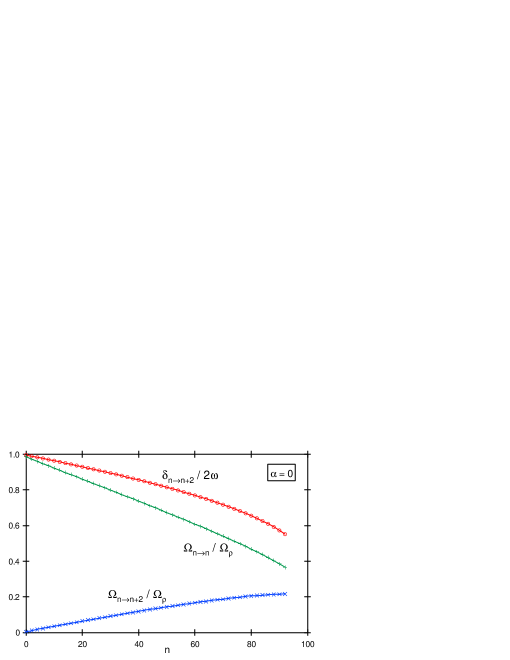
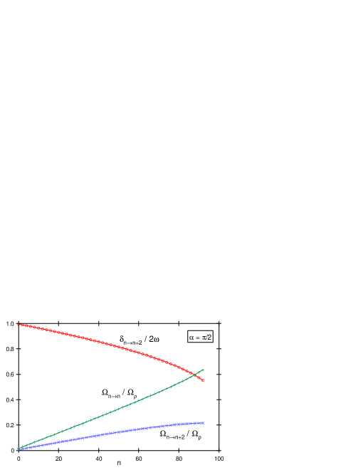
Figure 2: Rabi frequencies and detunings for FORT wells with $\alpha=0,\pi/2$: green curve is $\Omega_{n\rightarrow n}/\Omega_{\rho}$, blue curve is $\Omega_{n\rightarrow n+2}/\Omega_{\rho}$, red curve is $\delta_{n\rightarrow n+2}/2\omega$.

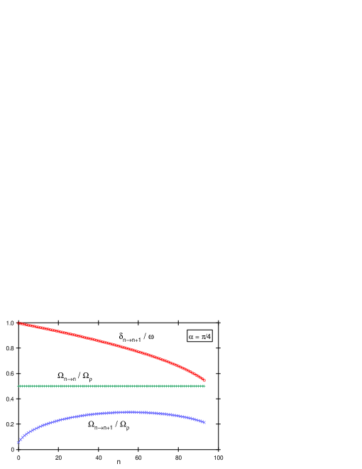
Figure 3: Rabi frequencies and detunings for FORT wells with $\alpha=\pi/4$: green curve is $\Omega_{n\rightarrow n}/\Omega_{\rho}$, blue curve is $\Omega_{n\rightarrow n+1}/\Omega_{\rho}$, red curve is $\delta_{n\rightarrow n+1}/\omega$.

V Raman coupling for cesium

V.1 Effective Hamiltonian

Figure 4: Level diagram for cesium.

So far we have discussed the FORT-Raman and Raman-Raman schemes in the context of a simple three-level model. In this section, we show how these schemes are modified when we take into account the multiplicity of levels in a physically realistic alkali atom, using cesium as an example.

A level diagram for cesium is shown in Figure 4; the levels relevant to our considerations include the ground state hyperfine manifolds $6S_{1/2},F=3$ and $6S_{1/2},F=4$, which correspond to ground states $a$ and $b$ of the three-level model, and the excited state manifolds $6P_{3/2}$ and $6P_{1/2}$, which correspond to the excited state $e$ of the three-level model. The Hamiltonian for a free cesium atom is

$$H_{0}=\sum_{e}\omega_{e}|e\rangle\langle e|+\frac{1}{2}\Delta_{HF}(P_{4}-P_{3}),$$ (54)

where the sum is taken over all the states $e$ in the $6P_{3/2}$ and $6P_{1/2}$ excited state manifolds, and where $P_{3}$ and $P_{4}$ are projection operators onto the $F=3$ and $F=4$ ground state manifolds. The quantity $\Delta_{HF}\equiv(2\pi)(9.2~{}\mathrm{GHz})$ is the hyperfine splitting between the $F=3$ and $F=4$ ground state manifolds, and $\omega_{e}$ is the energy of excited state $e$, where the zero of energy is taken to be halfway between the two ground state manifolds.

As in section III.1, we want to derive the Raman coupling that results when the atom is trapped within an optical cavity and one of the cavity modes is driven with a pair of beams that generate standing-wave fields inside the cavity. The coupling of the atom to the standing-wave fields is described by a Hamiltonian $H_{R}$ that has the same form as equation (14), but with $\hat{\Omega}_{\pm}$ given by

$$\hat{\Omega}_{\pm}=\gamma\,(I_{\pm}/I_{sat})^{1/2}\,\psi(\vec{r})\,\hat{\epsilon}_{\pm}^{*}\cdot\vec{A}.$$ (55)

Here $I_{\pm}$ are the maximum intensities of the two fields, and $\gamma=(2\pi)(5.2\,\mathrm{MHz})$ and $I_{sat}=2.19\,\mathrm{mW/cm^{2}}$ are the spontaneous decay rate and saturation intensity for the $6P_{3/2}$ excited state manifold. We can express $I_{sat}$ as

$$I_{sat}=(4\pi^{2}/3)(\gamma/\lambda_{D2}^{3}),$$ (56)

where $\lambda_{D2}=852\,\mathrm{nm}$ is the wavelength of the $6S_{1/2}\rightarrow 6P_{3/2}$ transition. The quantities $\hat{\epsilon}_{\pm}$ are the polarizations of the two fields, which we will take to be linear and mutually orthogonal. Thus, the vectors $\{\hat{\epsilon}_{+},\hat{\epsilon}_{-},\hat{k}\}$ form an orthonormal frame, where $\hat{k}$ is a unit vector that lies along the cavity axis. The vector $\vec{A}$ is an atomic lowering operator, and is defined by

$$\vec{A}^{\dagger}\equiv\sum_{J^{\prime}}\sum_{m^{\prime}}\sum_{m}\sum_{q=-1}^{1}\beta_{J^{\prime}}(F^{\prime},F)\,\langle F^{\prime},m^{\prime}|1,q;F,m\rangle\,|6P_{J^{\prime}},F^{\prime},m^{\prime}\rangle\langle 6S_{1/2},F,m|\,\hat{e}_{q}^{*}.$$ (57)

Here $\langle F^{\prime},m^{\prime}|1,q;F,m\rangle$ is the Clebsch-Gordan coefficient that connects ground state $|F,m\rangle$ to excited state $|F^{\prime},m^{\prime}\rangle$ via polarization $\hat{e}_{q}^{*}$,

$$\hat{e}_{0}=\hat{z},\qquad\hat{e}_{\pm 1}=\mp\frac{1}{\sqrt{2}}(\hat{x}\pm i\hat{y}),$$ (58)

is a orthonormal basis of polarization vectors, and

$$\beta_{J^{\prime}}(F,F^{\prime})=-(-1)^{F^{\prime}}\sqrt{2J^{\prime}+1}\sqrt{2F+1}\left\{\begin{array}[]{ccc}1&1/2&J^{\prime}\\ 7/2&F^{\prime}&F\end{array}\right\},$$ (61)

is a weighting factor for transitions between the $6S_{1/2},F$ and $6P_{J^{\prime}},F^{\prime}$ hyperfine manifolds, where the quantity in brackets is a $6J$-symbol.

Following the procedure we used in section III.1, we can adiabatically eliminate the excited states to obtain an effective Hamiltonian for the ground states. Because the derivation closely parallels the derivation given in section III.1, we will omit the intermediate steps and simply quote the result:

$$H_{E}=\frac{1}{2}\Delta_{HF}(P_{4}-P_{3})+\hat{V}_{E}+(\hat{\Omega}_{E}+\hat{\Omega}_{E}^{\dagger})\,\cos\delta_{R}t,$$ (62)

where

$$\hat{V}_{E} = \sum_{F}\sum_{e}\frac{1}{4\Delta_{e}}\,P_{F}\,(\hat{\Omega}_{+}|e\rangle\langle e|\hat{\Omega}_{+}^{\dagger}+\hat{\Omega}_{-}|e\rangle\langle e|\hat{\Omega}_{-}^{\dagger})P_{F},$$ (63)

$$\hat{\Omega}_{E} = \sum_{e}\frac{1}{2\Delta_{e}}\,P_{3}\,\hat{\Omega}_{+}|e\rangle\langle e|\hat{\Omega}_{-}^{\dagger}P_{4}.$$ (64)

Here $\Delta_{e}\equiv\omega_{L}-\omega_{e}$ is the overall detuning of the Raman pair from excited state $e$. In the limit that $\Delta_{e}$ is much larger than the excited state hyperfine splittings, one can show that boozer05

$$\sum_{e}\frac{1}{\Delta_{e}}A_{i}|e\rangle\langle e|A_{j}^{\dagger} = (1/3)[(2/\Delta_{D2}+1/\Delta_{D1})\,\delta_{ij}+2i(1/\Delta_{D2}-1/\Delta_{D1})\,\epsilon_{ijk}\,J_{k}],$$ (65)

where $\Delta_{D1}\equiv\omega_{L}-\omega_{D1}$ and $\Delta_{D2}\equiv\omega_{L}-\omega_{D2}$ are the overall detunings of the Raman pair from the cesium $D1$ and $D2$ lines. It is convenient to express these detunings as

$$1/\Delta_{D1}=-(\lambda_{L}/2\pi)\,C_{D1},\qquad 1/\Delta_{D2}=-(\lambda_{L}/2\pi)\,C_{D2},$$ (66)

where

$$C_{D1}\equiv(\lambda_{L}/\lambda_{D1}-1)^{-1},\qquad C_{D2}\equiv(\lambda_{L}/\lambda_{D2}-1)^{-1}$$ (67)

are dimensionless parameters. From equations (63), (64), and (65), we find that

$$\hat{V}_{E}=V_{E}\,|\psi(\vec{r})|^{2},\qquad\hat{\Omega}_{E}=\Omega_{E}\,|\psi(\vec{r})|^{2}\,\hat{\Sigma},$$ (68)

where

$$V_{E} \equiv (\gamma^{2}/12)((I_{+}+I_{-})/I_{sat})(2/\Delta_{D2}+1/\Delta_{D1}),$$ (69)

$$\Omega_{E} \equiv (\gamma^{2}/)(I_{+}I_{-}/I_{sat}^{2})^{1/2}(1/\Delta_{D2}-1/\Delta_{D1}),$$ (70)

and

$$\hat{\Sigma}\equiv 2\,P_{3}\,\hat{k}\cdot\vec{J}\,P_{4}$$ (71)

is an atomic lowering operator that couples Zeeman states in $F=4$ to Zeeman states in $F=3$. If we collect these results, make the rotating wave approximation, and perform a unitary transformation to eliminate the time-dependence, we can express the effective Hamiltonian as

$$H_{E}=-\frac{\delta}{2}(P_{4}-P_{3})-V_{E}\,|\psi(\vec{r})|^{2}+\frac{1}{2}\Omega_{E}\,|\psi(\vec{r})|^{2}\,(\hat{\Sigma}+\hat{\Sigma}^{\dagger}).$$ (72)

It is instructive to compare to the effective Hamiltonian for the three-level model given in equation (24) with the effective Hamiltonian for the full cesium atom given in equation (72). The two Hamiltonians have similar forms, only the operator $\sigma_{x}$ that coupled ground states $a$ and $b$ has been replaced by the operator $\hat{\Sigma}+\hat{\Sigma}^{\dagger}$ that couples Zeeman states within the ground state manifolds $F=3$ and $F=4$. In addition, we now have equations (69) and (70) that allow us to calculate the parameters $V_{E}$ and $\Omega_{E}$ in terms of the intensities of the standing-wave fields.

Following the same reasoning that was used in sections III.3 and III.2, we can use the effective Hamiltonian given in equation (72) to write down the total Hamiltonian $H$ for the FORT-Raman and Raman-Raman configurations. In both cases the total Hamiltonian has the form $H=H_{ext}+H_{int}$, where

$$H_{ext} = \frac{p^{2}}{2m}+U_{\rho}\,\sin^{2}k_{F}x,$$ (73)

$$H_{int} = -\frac{\delta}{2}(P_{4}-P_{3})+\frac{1}{2}\Omega_{\rho}\,\cos^{2}(k_{F}x+\alpha)\,(\hat{\Sigma}+\hat{\Sigma}^{\dagger}).$$ (74)

Here $U_{\rho}=U_{F}\,e^{-2\rho^{2}/w_{F}^{2}}$ and $\Omega_{\rho}=\Omega_{E}\,e^{-2\rho^{2}/w_{F}^{2}}$ are the axial trap depth and the effective Rabi frequency at radial coordinate $\rho$, and the parameters $U_{F}$ and $\Omega_{E}$ are calculated for the FORT-Raman and Raman-Raman configurations in the following sections V.2 and V.3.

V.2 FORT-Raman configuration

As was discussed in section III.2, in the FORT-Raman configuration the FORT forms one leg of the Raman pair, and a weak Raman beam is added to form the second leg. The FORT resonantly drives mode $n_{F}$ of the cavity, and the Raman beam drives the same mode as the FORT but is detuned from the cavity resonance by $|\delta_{R}|\sim\Delta_{HF}$.

We can obtain expressions for the FORT depth $U_{F}$ and the effective Rabi frequency $\Omega_{E}$ by using equations (69) and (70), which relate these quantities to the maximum intensities of the FORT and Raman beams inside the cavity, together with equation (102) from Appendix A, which relates these maximum intensities to the optical powers of the FORT and Raman beams at the input of the cavity (note that because the Raman beam is detuned from the cavity resonance, its coupling into the cavity is suppressed). We find that

$$U_{F} = (\gamma/24\pi)(\gamma/\kappa_{F})(2C^{F}_{D2}+C^{F}_{D1})(P_{F}/P_{c}),$$ (75)

$$\Omega_{E} = (\gamma/12\pi)(\gamma/\kappa_{F})(C^{F}_{D2}-C^{F}_{D1})(1+(2\Delta_{HF}/\kappa_{F})^{2})^{-1/2}(P_{R}P_{F}/P_{c}^{2})^{1/2}.$$ (76)

Here $P_{F}$ and $P_{R}$ are the powers of the FORT and Raman beams at the input of the cavity, $P_{c}$ is a reference power that is set by the cavity geometry and is defined in equation (101) of Appendix A, $\kappa_{F}$ is the total energy decay rate for the FORT mode $n_{F}$, and $C^{F}_{D2}$ and $C^{F}_{D1}$, the detuning parameters at the FORT wavelength $\lambda_{F}$, are given by equation (67). It is interesting to note that for fixed powers in the FORT and Raman beams, the effective Rabi frequency $\Omega_{E}$ monotonically increases as the cavity decay rate $\kappa_{F}$ is reduced.

In deriving the expression for $U_{F}$ given in equation (75), we assumed that the detuning of the FORT from the cesium $D1$ and $D2$ lines was the same for the $F=3$ and $F=4$ ground state hyperfine manifolds. This is a reasonable approximation, because these detunings are much larger than the hyperfine splitting $\Delta_{HF}$. However, because the detuning of the $F=3$ manifold is slightly larger than the detuning of the $F=4$ manifold, the FORT potential is slightly weaker for $F=3$. Thus, the FORT squeezes the two manifolds together, causing a small reduction in the effective hyperfine splitting. This effect, which is calculated in Appendix C, gives a slight position-dependence to the effective Raman detuning, but this can be neglected for many applications.

V.3 Raman-Raman configuration

As was discussed in section III.3, in the Raman-Raman configuration the FORT resonantly drives mode $n_{F}$ of the cavity, and pair of Raman beams drives mode $n_{R}$ of the cavity. We will assume that the two Raman beams have equal powers $P_{R}$ and are tuned symmetrically about the cavity resonance.

The FORT depth $U_{F}$ is given by equation (75), and we can obtain an expression for the Rabi frequency $\Omega_{E}$ by using equation (70), which relates the Rabi frequency to the maximum intensities of the Raman beams inside the cavity, together with equation (102) from Appendix A, which relates these maximum intensities to the optical powers of the Raman beams at the input of the cavity (note that because the Raman beams are detuned from the cavity resonance, their coupling into the cavity is suppressed). We find that

$$\Omega_{E}=(\gamma/12\pi)(\gamma/\kappa_{R})(C^{R}_{D2}-C^{R}_{D1})(1+(\Delta_{HF}/\kappa_{R})^{2})^{-1}(P_{R}/P_{c}).$$ (77)

Here $P_{c}$ is a reference power that is set by the cavity geometry and is defined in equation (101) of Appendix A, $\kappa_{R}$ is the total energy decay rate for the Raman mode $n_{R}$, and $C^{R}_{D2}$ and $C^{R}_{D1}$, the detuning parameters at the Raman wavelength $\lambda_{R}$, are given by equation (67). Note that for fixed powers in the Raman beams there is an optimal cavity decay rate $\kappa_{R}=\Delta_{HF}$ that maximizes the effective Rabi frequency $\Omega_{E}$.

V.4 Zeeman transitions

The operator $\hat{\Sigma}+\hat{\Sigma}^{\dagger}$ that appears in $H_{int}$ couples individual Zeeman transitions between the $F=3$ and $F=4$ ground state hyperfine manifolds. In this section, we calculate the matrix elements for these transitions.

Let us introduce an arbitrary coordinate system $\{\hat{x},\hat{y},\hat{z}\}$ and define a set of Zeeman states $\{|3,m\rangle,|4,m\rangle\}$ relative to this coordinate system. We can express the unit vector $\hat{k}$ that lies along the cavity axis as

$$\hat{k}=\cos\phi\sin\theta\,\hat{x}+\sin\phi\sin\theta\,\hat{y}+\cos\theta\,\hat{z},$$ (78)

where $\theta$ is the angle between the cavity axis $\hat{k}$ and the quantization axis $\hat{z}$. Note that

$$\hat{\Sigma}=2P_{3}\,\hat{k}\cdot\vec{J}\,P_{4}=P_{3}\,(2J_{z}\,\cos\theta+J_{+}\,e^{-i\phi}\sin\theta+J_{-}\,e^{i\phi}\sin\theta)\,P_{4},$$ (79)

where $J_{\pm}=J_{x}\pm iJ_{y}=\mp\sqrt{2}J_{\pm 1}$ are angular momentum raising and lowering operators. Thus, the state $|3,m\rangle$ couples to states $|4,m\rangle$ and $|4,m\pm 1\rangle$, and the matrix elements corresponding to these transitions are

$$\langle 4,m|\hat{\Sigma}^{\dagger}|3,m\rangle = (1-m^{2}/16)^{1/2}\,\cos\theta,$$ (80)

$$\langle 4,m+1|\hat{\Sigma}^{\dagger}|3,m\rangle = \frac{1}{8}(4+m)^{1/2}(5+m)^{1/2}\,e^{-i\phi}\,\sin\theta,$$ (81)

$$\langle 4,m-1|\hat{\Sigma}^{\dagger}|3,m\rangle = \frac{1}{8}(4-m)^{1/2}(5-m)^{1/2}\,e^{i\phi}\,\sin\theta,$$ (82)

where we have used that the matrix elements of $\vec{J}$ are given by boozer05

$$\langle F_{2},m_{2}|J_{q}|F_{1},m_{1}\rangle=-(3/2)^{1/2}\,(-1)^{F_{2}}\,\sqrt{2F_{1}+1}\,\left\{\begin{array}[]{ccc}1&1/2&1/2\\ 7/2&F_{2}&F_{1}\end{array}\right\}\,\langle F_{2},m_{2}|1,q;F_{1},m_{1}\rangle.$$ (85)

Note that if the quantization axis is aligned along the cavity axis then $\Delta m=\pm 1$ transitions are forbidden, and if the quantization axis is transverse to the cavity axis then $\Delta m=0$ transitions are forbidden.

VI Resolved-sideband cooling

VI.1 Cooling schemes

We have shown that the Raman coupling can drive transitions that raise or lower the axial vibrational quantum number $n$. In this section, we show how one can exploit these $n$-changing transitions to cool the axial motion to the vibrational ground state. We will first show how the cooling works using the three-level model, and then discuss cooling for a physically realistic cesium atom.

One way to cool the atom is to alternate coherent Raman pulses tuned to an $n$-lowering transition with incoherent repumping pulses. To see how this works, let us assume that we start out with the atom in state $|a,n\rangle$. We can lower the vibrational quantum number by driving the atom with a coherent Raman pulse tuned to the $n\rightarrow n-1$ transition, which transfers some of the population from $|a,n\rangle$ to $|b,n-1\rangle$. The atom can then be repumped to ground state $a$ by driving the $b-e$ transition with near-resonant light. The repumping light drives the atom to the excited state, from which it spontaneously decays to either ground state $b$, where it continues to interact with the repumping light, or to ground state $a$, where it is dark to the light. If the atom is sufficiently cold to begin with, then the repumping process is unlikely to change the atom’s vibrational state, because the matrix elements for $n$-changing transitions are suppressed relative to the matrix elements for $n$-preserving transitions by at least $\eta_{e}\sqrt{n}$, where $\eta_{e}\equiv(2m\omega)^{-1/2}\,\omega_{e}$. Thus, the net effect of the Raman and repumping pulses is to move some of the population from state $|a,n\rangle$ to state $|a,n-1\rangle$. By iterating the pulse sequence, the atom can be cooled to a state that has a mean vibrational quantum number $\bar{n}$ that is close to zero.

The same type of scheme can be used to cool a multi-level alkali atom. For a cesium atom, the $F=3$ ground state manifold plays the role of state $a$ and the $F=4$ ground state manifold plays the role of state $b$: we start with the atom in a random Zeeman state in $F=3$, drive the atom with a coherent Raman pulse tuned to the $n\rightarrow n-1$ transition, and then repump the atom to $F=3$. It is easiest to understand the effects of these pulses if we choose the quantization axis to lie along the cavity axis, so that only $\Delta m=0$ transitions are allowed and the Raman coupling drives transitions between pairs of states $|3,m\rangle\leftrightarrow|4,m\rangle$. If the ambient magnetic fields are nulled, then these Zeeman transitions are all degenerate, so the transition frequency of the $n\rightarrow n-1$ transition is independent of $m$. Thus, the coherent Raman pulse is effective at lowering the vibrational quantum number regardless of which Zeeman state in $F=3$ the atom started in: each Zeeman pair behaves equivalently, except for a slight $m$-dependence in the Rabi frequency that is given by equation (80). The Zeeman state of the atom is then scrambled during the repumping phase, so at the beginning of the next cooling cycle the atom starts out in a potentially new Zeeman state.

The amount of time it takes to cool the atom is determined by the amount of time it takes to repump the atom, which is set by the spontaneous decay rate of the excited state, and by the amount of time it takes to perform the coherent Raman pulse, which is set by the Rabi frequency $\Omega_{n\rightarrow n-1}$. The cooling rate can be increased by increasing the Rabi frequency, but as we increase the Rabi frequency we begin to off-resonantly drive the $n\rightarrow n$ transition, and this sets an upper limit to the Rabi frequency that can be used. Off-resonant driving of the $n\rightarrow n$ transition becomes important when $\Omega_{n\rightarrow n}\sim\omega$, so the upper limit to the Rabi frequency is given by $\Omega_{n\rightarrow n-1}\sim\eta\sqrt{n}\,\omega$.

There is also a lower limit to the value of $\bar{n}$ that can be achieved with this cooling scheme, which is set by two different factors. First, when we resonantly drive the $n\rightarrow n-1$ transition with the coherent Raman pulse, we can also off-resonantly drive the $n\rightarrow n+1$ transition. This mechanism gives a lower limit of $\bar{n}\sim(\Omega_{0\rightarrow 1}/2\omega)^{2}$. We can reduce this limit by reducing the Rabi frequency, but since the Rabi frequency determines the cooling rate, this also slows down the cooling. In addition, there are problems with using small Rabi frequencies that are due to the anharmonicity of the FORT, which will be discussed later. Ideally, one would gradually reduce the Rabi frequency as the atom cools, so as to balance the conflicting demands for a high cooling rate and a low value of $\bar{n}$. A second factor that limits $\bar{n}$ is the fact that when the atom is repumped it will not always remain in the same vibrational state it started out in, since the Lamb-Dicke suppression of $n$-changing transitions is not perfect. This mechanism gives a lower limit of $\bar{n}\sim\eta_{e}^{2}$.

The cooling scheme described above can be modified in several ways. First, rather than alternating Raman pulses with repumping pulses, it is also possible to continuously drive the atom with both Raman and repumping light, and this is the method that was used in boca04 and boozer06 . Second, the cooling scheme we described relies on $\Delta n=-1$ transitions, but it is also possible to cool the atom using $\Delta n=-2$ transitions. Indeed, for the FORT-Raman configuration the $\Delta n=-1$ transitions are forbidden, so the atom can only be cooled using $\Delta n=-2$ transitions. Cooling via $\Delta n=-2$ transitions tends to be slower than cooling via $\Delta n=-1$ transitions, since the condition $\Omega_{n\rightarrow n}\sim\omega$ gives an upper limit on the Rabi frequency of $\Omega_{n\rightarrow n-2}\sim\eta^{2}n\,\omega$. Also, for $\Delta n=-2$ transitions both the state $|a,0\rangle$ and the state $|a,1\rangle$ decouple from the Raman pulse, so the state to which the system cools depends on the initial state: if we start in a state $|a,n\rangle$ with $n$ even then the system cools to $|a,0\rangle$, and if we start in state $|a,n\rangle$ with $n$ odd then the system cools to $|a,1\rangle$.

Note that because the FORT is anharmonic, the resonant frequency of the $\Delta n=-1$ and $\Delta n=-2$ transitions depends on the value of $n$. This means that if we keep the Raman detuning $\delta$ set at at a fixed value throughout the cooling process, then the detuning of the Raman pulse from the atom will change as the atom cools. We can estimate the importance of this effect by considering $\Delta n=-1$ and $\Delta n=-2$ transitions as separate cases. First we will consider $\Delta n=-1$ transitions. Let us assume that we set the Raman detuning to $\delta=-\omega$, so the detuning of the Raman pulse from the $n\rightarrow n-1$ transition is

$$\Delta_{n\rightarrow n-1}=\delta-\delta_{n\rightarrow n-1}\sim\eta^{2}n\,\omega.$$ (86)

As we have shown, the maximum Rabi frequency that can be used is $\Omega_{n\rightarrow n-1}\sim\eta\sqrt{n}\,\omega$, and for this maximum value the ratio of the detuning to the Rabi frequency is $\sim\eta\sqrt{n}$, which is small for cold atoms. Thus, for $\Delta n=-1$ transitions the dependence of the detuning on $n$ is a small effect; we can simply set the Raman detuning to $\delta=-\omega$, and as long as the atoms start out reasonably cold the cooling will always be efficient.

Now consider $\Delta n=-2$ transitions. We will assume that the Raman detuning is set to $\delta=-2\omega$, so the detuning of the Raman pulse from the $n\rightarrow n-2$ transition is

$$\Delta_{n\rightarrow n-2}=\delta-\delta_{n\rightarrow n-2}\sim 2\eta^{2}n\,\omega.$$ (87)

As we have shown, the maximum Rabi frequency that can be used is $\Omega_{n\rightarrow n-2}\sim\eta^{2}n\,\omega$, and for this maximum value the ratio of the detuning to the Rabi frequency is $\sim 2$. Thus, for $\Delta n=-2$ transitions the dependence of the detuning on $n$ is a significant effect. To compensate for this problem, one could slowly decrease the Raman detuning $\delta$ during the cooling process to ensure that the Raman pulse remains in resonance as the atom cools.

Although we have focused on cooling the axial motion of the atom, it is possible to implement the axial cooling schemes in such a way that they cool the atom’s radial motion as well. This is accomplished by configuring the repumping light so that it provides polarization gradient cooling boiron96 in the plane transverse to the cavity axis. Specifically, the repumping light is tuned blue of the $6S_{1/2},F=4\rightarrow 6P_{3/2},F^{\prime}=4$ transition, and is delivered to the atom via two pairs of counter-propagating beams. The two pairs of beams are perpendicular to one another and to the cavity axis, and therefore provide cooling in both transverse directions.

VI.2 Measuring the temperature

One can characterize the effectiveness of the cooling schemes described in the previous section by using Raman spectroscopy to measure the temperature of the atom. In what follows, we will assume that $\Delta n=-1$ transitions are used to cool the atom, although the same methods can also be applied to cooling via $\Delta n=-2$ transitions.

To measure a Raman spectrum, we cool the atom, pump it into ground state $a$, and then drive it with a coherent Raman pulse with detuning $\delta$. We then check if the atom was transfered to $b$. By iterating this sequence one can measure the probability that the atom is transfered from $a$ to $b$ by the Raman pulse, and by repeating this measurement for Raman pulses of different detunings one can map out a Raman spectrum. For an atom in vibrational state $n$, the Raman spectrum will exhibit a peak at $\delta=0$, which corresponds to $n\rightarrow n$ transitions, and peaks at $\delta=\pm\delta_{n}$, which correspond to $n\rightarrow n\pm 1$ transitions. We will refer to the peak at $\delta=0$ as the carrier, and the peaks at $\delta=-\delta_{n}$ and $\delta=\delta_{n}$ as the red and blue sidebands. Because of the FORT anharmonicity $\delta_{n}$ depends on $n$, but we will assume that the atoms are cold enough that this effect can be neglected and simply take $\delta_{n}\simeq\omega$.

One way to determine the axial temperature of the atom is to measure the ratio of the red to the blue sideband; this is the same technique as was used in monroe95 to determine the temperature of a trapped ion. For a thermal distribution, the probability that the atom has axial vibrational quantum number $n$ is given by

$$P_{n}=\frac{1}{\bar{n}+1}\left(\frac{\bar{n}}{\bar{n}+1}\right)^{n},$$ (88)

where $\bar{n}\equiv(e^{\beta\omega}-1)^{-1}$ is the mean vibrational quantum number. If we start with the atom in state $a$ and resonantly drive the blue sideband with a Raman pulse of duration $t$, the probability that the atom is transfered to state $b$ is given by

$$p_{b}=\sum_{n=0}^{\infty}P_{n}\,\sin^{2}(\Omega_{n\rightarrow n+1}t/2).$$ (89)

If we start in state $a$ and resonantly drive the red sideband, the probability that the atom is transfered to state $b$ is given by

$$p_{r}=\sum_{n=1}^{\infty}P_{n}\,\sin^{2}(\Omega_{n\rightarrow n-1}t/2)=\sum_{n=0}^{\infty}P_{n+1}\,\sin^{2}(\Omega_{n+1\rightarrow n}t/2).$$ (90)

Note that

$$P_{n+1}=\left(\frac{\bar{n}}{\bar{n}+1}\right)\,P_{n},$$ (91)

so the ratio of the transfer probabilities for the red and blue sidebands is

$$p_{r}/p_{b}=\bar{n}/(\bar{n}+1).$$ (92)

An alternative way to quantify the cooling is to measure the population in the vibrational ground state. This can be accomplished by pumping the atom to state $a$ and applying a Raman pulse whose detuning is adiabatically swept across the red sideband. If the atom started in the vibrational ground state $n=0$ then it will remain in state $a$, and if the atom started in a vibrational state $n>0$ then the Raman pulse will adiabatically transfer it to state $b$. Thus, the population in the vibrational ground state is given by the probability that the atom remains in state $a$ after the adiabatic sweep has been completed. The advantage of this method is that it does not rely on assuming that the atoms are thermally distributed.

It is also possible to use Raman spectroscopy to say something about the radial temperature: since the axial frequency $\omega(\rho)=\omega_{a}\,e^{-\rho^{2}/w_{F}^{2}}$ depends on the radial coordinate $\rho$, the width of the sidebands depends on the radial temperature. The probability that the atom has axial frequency $\Delta$ is given by

$$p(\Delta)=\frac{1}{Z}\int_{0}^{\infty}e^{-\beta U(\rho)}\,\delta(\Delta-\omega(\rho))\,\rho\,d\rho,$$ (93)

where $U(\rho)=-U_{F}\,e^{-2\rho^{2}/w_{F}^{2}}$ is the potential for radial motion, and

$$Z=\int_{0}^{\infty}e^{-\beta U(\rho)}\,\rho\,d\rho.$$ (94)

If the radial temperature is small compared to the trap depth ($\beta U_{F}\gg 1$), then we can make a harmonic approximation and perform the integral analytically:

$$p(\Delta)=(1/\omega_{a})(2\beta U_{F})\,\theta(1-\Delta/\omega_{a})\,\exp(-2\beta U_{F}(1-\Delta/\omega_{a})).$$ (95)

Thus, if the blue sideband has width $\delta\omega$, one can put an upper limit on the radial temperature of $k_{B}T<2U_{F}(\delta\omega/\omega_{a})$.

VI.3 Cooling simulation

The cooling schemes discussed in section VI.1 can be simulated on a computer. We will take the Hamiltonian for the system to be

$$H=H_{int}+H_{ext}+H_{L},$$ (96)

where $H_{int}$ and $H_{ext}$ are given by equations (39) and (38), and where

$$H_{L}=-\Delta_{P}\,|e\rangle\langle e|+(\Omega_{P}/2)\,(|b\rangle\langle e|+|e\rangle\langle b|)$$ (97)

describes the coupling of the atom to repumping light. Here $\Omega_{P}$ is the Rabi frequency of the repumping light and $\Delta_{P}$ is the detuning of the light from the $b-e$ transition. As was discussed in section VI.1, in order to radially cool the atom we use light that is blue-detuned from the $4-4^{\prime}$ transition to repump the atom. To model this in the simulation, we will assume that the excited state decays to ground state $a$ at rate $\gamma_{a}=(5/12)\gamma$ and to ground state $b$ at rate $\gamma_{b}=(7/12)\gamma$, where $\gamma=(2\pi)(5.2\,\mathrm{MHz})$ is the spontaneous decay rate for the $6P_{3/2}$ manifold of cesium, and the prefactors $5/12$ and $7/12$, the branching ratios for spontaneous decay on the $6P_{3/2},F=4\rightarrow 6S_{1/2},F=3$ and $6P_{3/2},F=4\rightarrow 6S_{1/2},F=4$ transitions, are given by equation (61). Also, we will take $\Delta_{P}=(2\pi)(10\,\mathrm{MHz})$ to be the detuning that optimizes the polarization-gradient cooling.

We can write down a master equation for the system, which describes both the coherent evolution due to $H$ and the incoherent evolution due to the spontaneous decay from the excited state. Given an initial state, we can numerically integrate the master equation to obtain the state of the system at later times. In Figure 5a, we use this method to simulate cooling in the Raman-Raman configuration: we start the system in state $|a,5\rangle$ and plot $\bar{n}$ as a function of time. We assume that the atom is trapped in a FORT well with $\alpha=\pi/4$, and use $\Delta n=-1$ transitions to perform the cooling. For this simulation, the cooling parameters are $\Omega_{\rho}=(2\pi)(0.2\,\mathrm{MHz})$, $\Omega_{P}=-(2\pi)(3\,\mathrm{MHz})$, $\delta=-(2\pi)(0.5\,\mathrm{MHz})$. In Figure 5b, we simulate cooling in the FORT-Raman configuration. In the FORT-Raman configuration $\alpha=0$ for all the FORT wells and the $\Delta n=-1$ transitions are forbidden, so we use $\Delta n=-2$ transitions to perform the cooling. As was previously discussed, this means that the asymptotic state to which the system cools depends on the initial state. Two curves are shown in the graph: for one, we start the system in state $|a,3\rangle$; for the other, we start the system in state $|a,4\rangle$. For these simulations, the cooling parameters are $\Omega_{\rho}=(2\pi)(0.2\,\mathrm{MHz})$, $\Omega_{P}=-(2\pi)(3\,\mathrm{MHz})$, $\delta=-(2\pi)(0.75\,\mathrm{MHz})$.

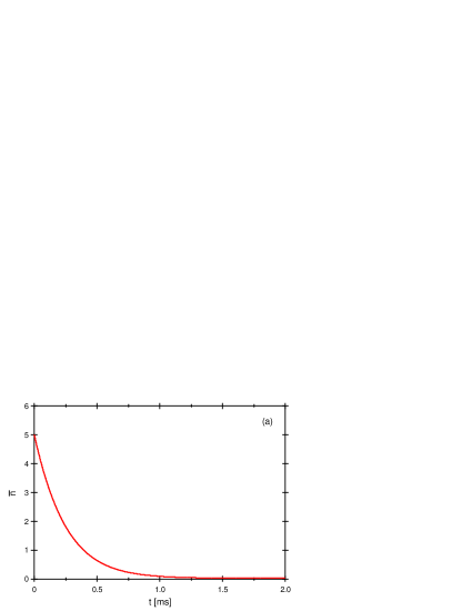
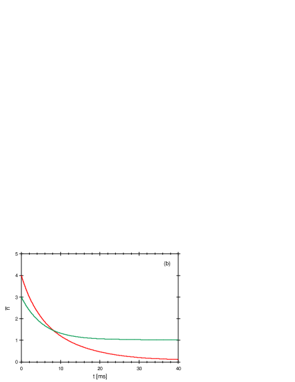
Figure 5: Cooling simulation: mean vibrational quantum number $\bar{n}$ versus time $t$, (a) cooling via $\Delta n=-1$ transitions starting from state $|a,5\rangle$, (b) cooling via $\Delta n=-2$ transitions starting from states $|a,3\rangle$ and $|a,4\rangle$.

In addition to simulating the time-evolution of the system, we can calculate the asymptotic value of $\bar{n}$ by solving the master equation for the steady-state density matrix. This can be used to study the dependence of the asymptotic value of $\bar{n}$ on the various cooling parameters. In Figure 6, we consider cooling in the Raman-Raman configuration for atoms with $\pi/4$, and plot the asymptotic value of $\bar{n}$ as a function of $\Omega_{\rho}$, $\Omega_{P}$, and $\delta$. The parameters that are not being varied are set to the same values used for the cooling simulation shown in Figure 5a. These graphs show that the cooling scheme is quite robust and works efficiently over a broad range of parameters.

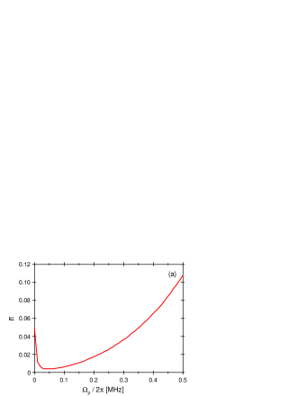
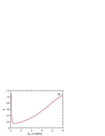
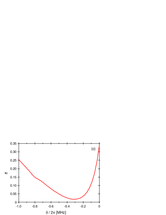
Figure 6: Cooling simulation: (a) asymptotic $\bar{n}$ versus $\Omega_{\rho}$, (b) asymptotic $\bar{n}$ versus $\Omega_{P}$, (c) asymptotic $\bar{n}$ versus $\delta$.

VII Conclusion

We have described two schemes for driving Raman transitions in an atom trapped within a high-finesse optical cavity. These schemes can be used to control both the internal and motional degrees of freedom of the atom, and provide powerful tools for studying cavity QED; as an example, we have shown in detail how the Raman schemes can be used to cool the atom to the quantum ground state of the trapping potential. Although the two schemes are similar in many respects, they do have some important differences. The FORT-Raman scheme has the advantage that the Raman coupling is independent of the FORT well in which the atom is trapped, and is thus better suited for manipulating the internal state of the atom. On the other hand, the Raman-Raman scheme has the advantage that the $n\rightarrow n\pm 1$ transitions are allowed for most FORT wells, and is thus better suited for cooling. The ability to coherently control the atom is a key requirement for many cavity QED protocols, and these Raman schemes should open up new possibilities for experiments in cavity QED.

Appendix A Cavity mode structure

Here we describe the mode structure of the optical cavity. The cavity we will be considering consists of two symmetric mirrors of radius $R$ that are separated by a distance $L$. It is convenient to define a cylindrical coordinate system that is centered on the cavity axis: we will denote the distance from the cavity axis by $\rho$ and the displacement along the cavity axis by $z$, where the mirrors are located at $z=0$ and $z=L$. The cavity supports a set of discrete modes with resonant frequencies at integer multiples of the free spectral range $\nu_{FSR}=1/2L$, where for each frequency there are two degenerate modes corresponding to the two polarization states transverse to the cavity axis. Consider one of the polarization modes with mode order $n$. We will let $\omega=2\pi n\nu_{FSR}$ denote the resonant frequency of the mode, and let $\lambda=2\pi/\omega$ and $k=2\pi/\lambda$ denote the corresponding wavelength and wavenumber. We can characterize the shape of the mode by a dimensionless function $\psi(\vec{r})$ that is given by

$$\psi(\vec{r})=e^{-\rho^{2}/w^{2}}\,\sin kz,$$ (98)

where $w=(L(2R-L)/k^{2})^{1/4}$ is the mode radius. If we drive the cavity with an input beam that has power $P_{i}$ and frequency $\omega_{i}$, then the intensity at a point $\vec{r}$ inside the cavity is

$$I(\vec{r})=(2/\kappa V)(1+(2\Delta/\kappa)^{2})^{-1}\,|\psi(\vec{r})|^{2}\,P_{i},$$ (99)

where $\Delta=\omega_{i}-\omega_{c}$ is the detuning of the input beam from the cavity resonance, $\kappa$ is the total energy decay rate for the mode, and $V$, the mode volume, is given by

$$V=\int|\psi(\vec{r})|^{2}\,d^{3}r=(\lambda L/8)(2RL)^{1/2}.$$ (100)

In order to relate the input power to the maximum intensity inside the cavity, it is convenient to define a power

$$P_{c}\equiv(2V/\lambda)I_{sat}=(L/4)(2RL)^{1/2}\,I_{sat}.$$ (101)

Note that $P_{c}$ is the same for all cavity modes; it depends only on the cavity geometry, not the mode number. We can then express the maximum intensity inside the cavity as

$$I_{max}=(\kappa\lambda)^{-1}\,(1+(2\Delta/\kappa)^{2})^{-1}\,(P_{i}/P_{c})\,I_{sat}.$$ (102)

Appendix B Distortion of the trapping potential

In the Raman-Raman configuration, the lack of registration between the FORT and Raman beams causes a well-dependent distortion of the trapping potential. Here we calculate this effect. From equation (32), we see that the total potential for the Raman-Raman configuration is given by

$$U(\vec{r})=-U_{F}\,e^{-2\rho^{2}/w_{F}^{2}}\,\sin^{2}k_{F}z-U_{R}\,e^{-2\rho^{2}/w_{R}^{2}}\,\sin^{2}k_{R}z.$$ (103)

We will assume that an atom is trapped in well $r$ of the FORT, and define a coordinate $x=z-z_{r}$ and a phase $\alpha=(k_{R}-k_{F})z_{r}$. Note that

$$\sin^{2}k_{F}z=\cos^{2}k_{F}x,\qquad\sin^{2}k_{R}z=\cos^{2}(k_{R}x+\alpha).$$ (104)

We will assume that the FORT and Raman beams drive nearby modes of the cavity, so $|k_{R}-k_{F}|\ll k_{R},k_{F}$. In this limit, we can approximate $U(\vec{r})$ by replacing $w_{R}$ with $w_{F}$ and replacing $k_{R}x$ with $k_{F}x$:

$$U(\vec{r})=-U_{F}\,e^{-2\rho^{2}/w_{F}^{2}}\,\cos^{2}k_{F}x-U_{R}\,e^{-2\rho^{2}/w_{F}^{2}}\,\cos^{2}(k_{F}x+\alpha).$$ (105)

As in section II, we will take the atom to be radially stationary, and take $\rho$ as a constant parameter that enters into the potential for axial motion. We can then write the potential as

$$U(\vec{r})=U_{\rho}\,\sin^{2}(k_{F}x+\theta),$$ (106)

where $U_{\rho}\equiv U_{0}\,e^{-2\rho^{2}/w_{F}^{2}}$ is the axial trap depth at radial coordinate $\rho$. The quantity $U_{0}$ is given by

$$U_{0}=(U_{F}^{2}+2U_{F}U_{R}\cos 2\alpha+U_{R}^{2})^{1/2},$$ (107)

and $\theta$ is given by

$$\tan 2\theta=(U_{F}+U_{R}\cos 2\alpha)^{-1}U_{R}\sin 2\alpha.$$ (108)

Appendix C Differential Stark shift

The FORT potential is slightly weaker for the $F=3$ ground state manifold than for the $F=4$ ground state manifold, so there is a small differential Stark shift. Here we calculate this effect. The Hamiltonian that describes the differential Stark shift is

$$H_{D}=\frac{1}{2}\delta_{D}\,|\psi_{F}(\vec{r})|^{2}\,(P_{4}-P_{3})=H_{D}=\frac{1}{2}\delta_{\rho}\,(P_{4}-P_{3})\cos^{2}k_{F}x,$$ (109)

where $\delta_{D}$ is the differential Stark shift at an intensity maximum and $\delta_{\rho}\equiv\delta_{D}\,e^{-2\rho^{2}/w_{F}^{2}}$ is the maximum differential Stark shift at radial position $\rho$. We can calculate $\delta_{D}$ as follows. The FORT depth $U_{F}$ is given by (69) with $I_{+}=I_{F}$ and $I_{-}=0$:

$$U_{F}=(\gamma^{2}/12)(I_{F}/I_{sat})(2/\Delta_{D2}^{F}+1/\Delta_{D1}^{F}).$$ (110)

Thus, the differential Stark shift at an intensity maximum is given by

$$\delta_{D}=\frac{\gamma^{2}}{12}\frac{I_{F}}{I_{sat}}\left(\frac{2}{\Delta_{D2}^{F}}+\frac{1}{\Delta_{D1}^{F}}\right)-\frac{\gamma^{2}}{12}\frac{I_{F}}{I_{sat}}\left(\frac{2}{\Delta_{D2}^{F}+\Delta_{HF}}+\frac{1}{\Delta_{D1}^{F}+\Delta_{HF}}\right).$$ (111)

Expanding to first order in $\Delta_{HF}$, we find that

$$\delta_{D}=-U_{F}\,(2(C_{D2}^{F})^{2}+(C_{D1}^{F})^{2})(2C_{D2}^{F}+C_{D1}^{F})^{-1}\,(\Delta_{HF}/\omega_{F}).$$ (112)

where $C_{D1}^{F}$ and $C_{D2}^{F}$, the detuning parameters at the FORT wavelength $\lambda_{F}$, are given by equation (67).

References

- (1) J. Ye et al., Phys. Rev. Lett. 83, 4987 (1999).
- (2) J. McKeever et al., Phys. Rev. Lett. 90, 133602 (2003).
- (3) P. Maunz et al., Nature 428, 50 (2004).
- (4) J. A. Sauer et al., Phys. Rev. A 69, 051804(R) (2004).
- (5) S. Nußmann et al., Nature Physics 1, 122 (2005).
- (6) R. Miller et al., J. Phys. B 38, S551 (2005).
- (7) G. R. Guthöhrlein et al., Nature 414, 49 (2001).
- (8) A. B. Mundt et al., Phys. Rev. Lett. 89, 103001 (2002).
- (9) B. G. Englert et al., Europhys. Lett. 14, 25 (1991).
- (10) S. Haroche et al., Europhys. Lett. 14, 19 (1991).
- (11) M. J. Holland et al., Phys. Rev. Lett.67, 1716 (1991).
- (12) A. M. Herkommer et al., Phys. Rev. Lett. 69, 3298 (1992).
- (13) P. Storey, M. Collett, and D. F. Walls, Phys. Rev. Lett. 68, 472 (1992).
- (14) W. Ren et al., Phys. Rev. A 51, 752 (1995).
- (15) A. M. Herkommer et al., Quant. Sem. Opt. 8, 189 (1996).
- (16) M. O. Scully et al., Phys. Rev. Lett. 76, 4144 (1996).
- (17) T. Pellizzari et al., Phys. Rev. Lett. 75, 3788 (1995).
- (18) L.-M. Duan et al., Phys. Rev. Lett. 92, 127902 (2004).
- (19) J. I. Cirac et al., Phys. Rev. Lett. 78, 3221 (1997).
- (20) H.-J. Briegel et al., in The Physics of Quantum Information, edited by D. Bouwmeester et al., p. 192.
- (21) I. Dotesenko et al., Appl. Phys. B. 78, 711 (2004).
- (22) P. Clade et al., Phys. Rev. Lett. 96, 033001 (2006).
- (23) T.L. Gustavson, P. Bouyer, and M.A. Kasevich, Phys. Rev. Lett. 78, 2046 (1997).
- (24) D. J. Wineland et al., Phil. Trans. Royal Soc. London A 361, 1349 (2003).
- (25) C. Monroe et al., Phys. Rev. Lett. 75, 4011 (1995).
- (26) D. Leibfried et al., Rev. Mod. Phys. 75, 281 (2003).
- (27) S.E. Hamann et al., Phys. Rev. Lett. 80, 4149 (1998).
- (28) H. Perrin et al., Europhys. Lett. 42, 395 (1998).
- (29) V. Vuletic et al., Phys. Rev. Lett. 81, 5768 (1998).
- (30) A. Boca et al., Phys. Rev. Lett. 93, 233603 (2004).
- (31) A. D. Boozer et al., Phys. Rev. Lett. 97, 083602 (2006).
- (32) A. D. Boozer et al., Phys. Rev. A 76, 063401 (2007).
- (33) A. D. Boozer, Ph.D. thesis, California Institute of Technology, 2005.
- (34) D. Boiron et al., Phys. Rev. A 53, R3734 (1996).