Kondo effect and channel mixing in oscillating molecules

Abstract

We investigate the electronic transport through a molecule in the Kondo regime. The tunneling between the electrode and the molecule is asymmetrically modulated by the oscillations of the molecule, i.e., if the molecule gets closer to one of the electrodes the tunneling to that electrode will increase while for the other electrode it will decrease. We describe the system by a two-channel Anderson model with phonon-assisted hybridization. The model is solved with the Wilson numerical renormalization group method. We present results for several functional forms of tunneling modulation. For a linearized modulation the Kondo screening of the molecular spin is caused by the even or odd conduction channel. At the critical value of the electron-phonon coupling an unstable two-channel Kondo fixed point is found. For a realistic modulation the spin at the molecular orbital is Kondo screened by the even conduction channel even in the regime of strong coupling. A universal consequence of the electron-phonon coupling is the softening of the phonon mode and the related instability to perturbations that break the left-right symmetry. When the frequency of oscillations decreases below the magnitude of such perturbation, the molecule is abruptly attracted to one of the electrodes. In this regime, the Kondo temperature is enhanced and, simultaneously, the conductance through the molecule is suppressed.

I INTRODUCTION

The Kondo effect, a generic name for processes related to an increased scattering rate off impurities with internal degrees of freedom, reveals itself in mesoscopic systems as increased conductance at biases and temperatures low compared to the Kondo temperature. It has been observed in measurements of transport through quantum dotsGoldhaber-Gordon et al. (1998), atoms, and moleculesMadhavan et al. (1998); Liang et al. (2002); Park et al. (2002); Yu and Natelson (2004); Pasupathy et al. (2005); Zhao et al. (2005); Yu et al. (2005). Specific to molecules is the coupling of electrons to molecular oscillations. The molecular internal vibrational modes and oscillations of molecules with respect to the electrodes have been proposed to account for the side-peaks in the non-linear conductancePark et al. (2002); Yu and Natelson (2004); Pasupathy et al. (2005). In addition, the electron-phonon coupling can explain the anomalous dependence of the Kondo temperature on changing the gate voltage at zero bias Yu et al. (2005); Balseiro et al. (2006); Nuñez Regueiro et al. (2007); Cornaglia et al. (2007). Since the electrode-molecule junctions are candidates for devices such as molecular diodes, switches, and rectifiers the research in this field is increasing despite its complexity and the difficult experimental characterization Nitzan and Ratner (2003); Tao (2006); Galperin et al. (2007). Recently, also the notion of quantum phase transition was introduced in the analysis of such systemsRoch et al. (2008). We believe that for the interpretation of the experimental results a better understanding of the behavior of simple theoretical models is necessary.

Here we study the influence of the electron-phonon coupling in the Kondo regime where a single molecular orbital is occupied on average by one electron. We concentrate on the case where the oscillations of the molecule with respect to the electrodes affect the tunneling as depicted schematically in Fig. 1. That is, the tunneling toward the left and right electrodes is given by overlap integrals $V_{L,R}(x)$ that are modulated by the displacement $x$ of the molecule from the mid-point between the electrodes asymmetrically: $V_{R}$ increases and $V_{L}$ decreases for $x$ positive, and opposite for $x$ negative.

Assuming the electrodes are identical, it is convenient to introduce symmetric and antisymmetric combinations of states in the electrodes. With respect to inversion, they form even and odd conduction channels. The odd channel is coupled to the molecule only due to the asymmetric modulation of tunneling. For example, in the linear approximation $V_{L,R}(x)=V(1\mp gx)$ – a prefactor $V$ sets the intensity of the tunneling and the electron-phonon coupling constant $g$ its variation due to the displacementBarišić et al. (1970) – the even channel is coupled to the molecule directly and the odd channel is coupled to the molecule via a term proportional to $gx$.

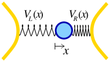
Figure 1: (Color online) Schematic plot of the model device.

As a consequence of coupling the molecular orbital to two channels the low-energy behavior is that of the two-channel Kondo (2CK) modelNozières and Blandin (1980); Balseiro et al. (2006). The screening of the spin occurs in the channel with the larger coupling constant. If the couplings match, an overscreened, i.e., a genuine 2CK problem with a non-Fermi liquid behaviour results. For a linearized model such a fixed point has indeed been found with simulations based on numerical renormalization groupMravlje et al. (2008).

Of interest is also the renormalization of phonon frequencies. Quite generally, the characteristic frequency of the oscillations decreases with increasing electron-phonon coupling. In the Anderson-Holstein model the softening of the phonon mode is related to the increased charge susceptibility Hewson and Meyer (2002); Mravlje et al. (2005), which occurs due to dynamical breaking of the particle-hole symmetry for negative effective repulsion $U$. In the present case the softening occurs as well and it is related to the dynamical breaking of inversion symmetryBalseiro et al. (2006). Due to the softening, the instability towards perturbations breaking the symmetry emerges. On the mean field levelMravlje et al. (2006), the instability is seen as an asymmetric ground state with large average $x$ in systems with inversion symmetry.

In this work we extend the existing analysis in two ways. (i) Motivated by the lack of the inversion symmetry of typical experimental devices we include the inversion symmetry breaking perturbation. (ii) We check which features persist if the tunneling is taken to depend exponentially on the displacement: $V_{L,R}(x)\propto\exp(\mp gx)$. In particular, it is shown that the softening of the phonon mode and the corresponding instability occur universally but the 2CK fixed point appears as an artifact of the linearization only. It is shown also that the softening is due to the kinetic energy gained by the dynamical breaking of inversion symmetry and that it occurs also for vanishing repulsion, $U\to 0$.

Both directions of research have been pursued in the context of nano-electromechanical systemsNovotný et al. (2004); Twamley et al. (2006); Johansson et al. (2008), where only the lowest orders in tunneling are considered and the Kondo correlations are thus lost. A similar approach has been followed in analyzing the influence of pair tunneling for negative effective $U$ in the Anderson-Holstein modelKoch et al. (2006); Hwang et al. (2007). On the other hand, the influence of the exponential dependence of tunneling rates on $x$ in the Kondo regime has been analyzed in Ref. Kiselev et al., 2006. However, the displacement $x$ is not treated as a dynamical variable there but only as an external control parameter.

The paper is organized as follows. In the next section we describe in more detail the models under consideration. We have performed the numerical calculations using Wilson’s numerical renormalization group (NRG) and projection operator method of Schönhammer and Gunnarsson (SG) which we briefly describe in Section III. In Section IV we present analytical and in Section V numerical results. We conclude by critically commenting the obtained results and their applicability. A comparison between the NRG and SG results is given in Appendix A followed by Appendices B and C containing the derivations of the Schrieffer-Wolff transformation and the conductance formulas.

II Models

We model the system with the Hamiltonian

$$H=H_{\mathrm{mol}}+H_{L}+H_{R}+H_{\mathrm{vib}}+H^{\prime},$$ (1)

where $H_{\mathrm{mol}}$ describes an isolated molecule, $H_{L}$ and $H_{R}$ the left and the right electrode, respectively, $H_{\mathrm{vib}}$ a vibrational mode and $H^{\prime}$ the phonon-assisted coupling of the molecular orbital to the electrodes. The molecule consists of a single orbital with energy $\epsilon$, which is in experiment modulated by the gate voltage. The repulsion between two electrons simultaneously occupying the orbital is $U$,

$$H_{\mathrm{mol}}=\epsilon(n_{\uparrow}+n_{\downarrow})+Un_{\uparrow}n_{\downarrow},$$ (2)

where the number operators $n_{\sigma}=d_{\sigma}^{\dagger}d_{\sigma}$ count the number of electrons in the orbital with spin $\sigma=\uparrow,\downarrow$. The symbols $c^{(\dagger)},d^{(\dagger)}$ denote electron annihilation (creation) operators in the electrodes and molecular orbital, respectively. We are here interested in the particle-hole symmetric point $\epsilon=-U/2$ only. The oscillator part is

$$H_{\mathrm{vib}}=\Omega a^{\dagger}a,$$ (3)

describing the oscillations with frequency $\Omega$ and $a^{\dagger}$ is the boson creation operator. The left and right electrodes are described by bands of noninteracting electrons $H_{\alpha}=\sum_{k\sigma}\epsilon_{k}n_{k\alpha\sigma}$ for $\alpha=L,R$, respectively, where $n_{k\alpha\sigma}=c^{\dagger}_{k\alpha\sigma}c_{k\alpha\sigma}$ counts the electrons with spin $\sigma$ and wave vector $k$; $\epsilon_{k}$ is the dispersion of the band in the electrode $\alpha$. The chemical potential is set to the middle of the band ($\mu=0$) corresponding to the half-filled regime where the molecule is on average singly occupied. In NRG calculations a flat band with constant density of states $\rho=1/(2D)$ and in SG calculations a tight-binding band with $\rho(\omega)=1/\left(\pi\sqrt{D^{2}-\omega^{2}}\right)$ are used, where $D$ is the half-width of the band.

The tunneling between the molecular orbital and the electrodes, which is described by

$$H^{\prime}=V_{L}(x)\widehat{v}_{L}+V_{R}(x)\widehat{v}_{R},$$ (4)

occurs via the hybridization operators (assuming here the tunneling is $k$-independent)

$$\widehat{v}_{\alpha}=\sum_{k\sigma}c_{k\alpha\sigma}^{\dagger}d_{\sigma}+h.c.$$ (5)

multiplied by the overlap integrals $V_{\alpha}(x)\equiv V_{\alpha}(a+a^{\dagger})$, where the displacement is explicitly quantized.

It is practical to define even and odd combinations of states in the electrodes, respectively

$$c^{\dagger}_{ke(o)\sigma}=\frac{1}{\sqrt{2}}\left(c^{\dagger}_{kL\sigma}\pm c^{\dagger}_{kR\sigma}\right).$$ (6)

In this basis $H^{\prime}$ reads

$$H^{\prime}=V_{e}(x)\widehat{v}_{e}+V_{o}(x)\widehat{v}_{o}$$ (7)

where

$$V_{e,o}(x)=\frac{V_{L}(x)\pm V_{R}(x)}{\sqrt{2}},$$ (8)

modulate the tunneling to even and odd channels. Hybridization operators $\widehat{v}_{e,o}$ correspond to Eq. (5) for $\alpha=e,o$, respectively. Note that

$$|V_{e}(x)|>|V_{o}(x)|$$ (9)

if $V_{L,R}(x)$ are both positive or both negative for all $x$.

In this paper we perform the calculations using several functional forms of $V_{\alpha}(x)$ depicted in Fig. 2.

II.1 Overlap integrals

In a realistic experimental situation the tunneling between the molecule and the tip of an electrode will be saturated at small distances and it will progressively decrease with increasing distance of the molecule from the electrode. The precise functional dependence of overlap integrals will in general depend on details of the molecule and the tips of the electrodes, but the overall behavior should be as shown in Fig. 2(a) with dotted line.

II.1.1 Linear modulation

The simplest form of overlap integrals is obtained by the expansion to lowest order in displacement resulting in linear modulation (LM)

$$V_{L,R}(x)=V\left[1\mp(gx+\zeta)\right].$$ (10)

The tunneling matrix element, constant $V$ for $g=0$, is linearly modulated by displacement for $g>0$. We assume the system is almost inversion symmetric. A small $\zeta\geq 0$ is the magnitude of the symmetry breaking perturbation. In the symmetrized basis the overlap integrals take on the following form

$$V_{e}=\sqrt{2}V,\;\;V_{o}=\sqrt{2}V(gx+\zeta).$$ (11)

Note that Eq. (11) does not satisfy the requirement Eq. (9) for $gx>1-\zeta$, because the overlap to the left electrode becomes negative and its absolute value starts to increase with increasing $x$ (dashed region in Fig. 2).

II.1.2 Exponential modulation

A better approximation to the overlap integrals could be exponential decay at large distances and arguably more realistic model is given with the exponential modulation (EM) of tunneling by

$$V_{L,R}(x)=V\left[\exp(\mp gx)\mp\zeta\right],$$ (12)

or equivalently

$$V_{e}=\sqrt{2}V\cosh(gx),\>\>V_{o}=\sqrt{2}V\left[\sinh(gx)+\zeta\right],$$ (13)

which are positive and for $\zeta=0$ manifestly satisfy the relation Eq. (9). By expanding the couplings to lowest order in $x$, the LM is recovered.

The EM eliminates the negative overlap but introduces another problem due to divergence of $\exp(gx)$ at large $gx$. Namely, the model with EM is unstable towards large displacements as can be understood by the following simple argument. For large $x$, the largest energies in the problem are $V\exp(gx)$ and $\Omega x^{2}$. This limit corresponds to two sites coupled by a tunneling term with tunneling proportional to $\exp(gx)$. The total energy of one electron on these two sites is $E\sim\Omega x^{2}/4-V\exp(gx)$. Therefore the oscillator in the EM moves in an effective potential of the form depicted in Fig. 2(b) (full), unbounded from below for large $|x|$.

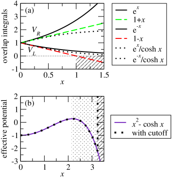
Figure 2: (Color online) (a) Various forms of the tunneling-modulation. The unphysical regime of LM where the tunneling starts to increase with increasing distance to the electrode is indicated by dashing. (b) The breakdown of EM. In the right-hand part the effective potential drops without bounds. This is regularized by the phonon cutoff, which corresponds to the hard-wall boundary. Two different cutoff regimes are indicated by dotted and dashed area.

II.2 Limitations of models

In real systems, the overlap integrals will be neither negative nor divergent. The large $x$ behaviour of EM can be corrected by adding higher terms in displacement to the oscillator potential, which corresponds to hardening of the ’spring’ for large $x$. In our numerical calculations such a hardening is incorporated in the form of a phonon cutoff which acts as a hard-wall boundary, thereby eliminating the states corresponding to displacements larger than $\sim 2\sqrt{L}$, where $L$ is the maximal number of phonons allowed. In Fig. 2(b), the dotted and the dashed regions indicate two different cutoff regimes. For the larger cutoff also the resulting effective potential is sketched (dotted).

By incorporating the cutoff into EM the results qualitatively depend on additional parameter $L$ because the choice of cutoff determines the form of the effective potential near low energies. However, without some kind of a regularization of the model the model with EM is ill defined; we show later that the average displacement (or its fluctuations for $\zeta=0$) diverge for all $g>0$ at $L\to\infty$.

We note that there may be several cases, where the modulation is not a simple function. To describe the experimental situation, it might even be needed to include the anharmonicity of the potential as well. However, a convenient starting point is to first clarify specific regimes of simplified models and the consequences of the approximations. In this paper, we first analyze the model with LM comprehensively. Later we discuss EM for a specific phonon cutoff to highlight which of the results obtained using LM are artifacts of the linearization. Finally, the exponential divergence of overlap integrals is regularized, Fig. 2(a) (dotted), and it is shown which results persist also for this model.

III Numerical methods

Most of the numerical results presented here have been obtained using the Wilson numerical renormalization groupWilson (1975); Bulla et al. (2008)(NRG) method. The NRG procedure is based on adding sites to the system iteratively with hopping matrix element to the $n$th added site decreasing as $\Lambda^{-n/2}$. At each step the resulting Hamiltonian is diagonalized and lowest $K$ eigenstates are kept. The exponentially decreasing hopping is essential to introduce all the energy scales while still keeping the numerical effort reasonable. Such a procedure is especially suitable for the Kondo problem where a range of energy scales contributes equally to the screening of the impurity spin. The algorithm is stopped after $N_{\mathrm{max}}$ iterations. In the presented results we have typically used $\Lambda=3-4$, $K=2000$ (not counting the degeneracies due to spin, isospin, and parity symmetriesŽitko and Bonča (2006) which have been explicitly taken into account) and $N_{\mathrm{max}}=40$.

In order to gain additional insight and to make a relation with our previous work we compare the NRG results to the results obtained by the Schönhammer-Gunnarsson (SG) Schönhammer (1976); Gunnarsson and Schönhammer (1985) variational method. The details of our implementation of the variational method are given in our previous work Rejec and Ramšak (2003a, b); Mravlje et al. (2005). For reader’s convenience we here just remark that it consists of finding the parameters of an auxiliary noninteracting Hamiltonian $\tilde{H}$ [of the same form as $H$ in Eq. (1), but for $g=0,U=0$ and described by renormalized parameters $\tilde{V}_{L},\tilde{V}_{R},\tilde{\epsilon}$], which minimize the variational ground state energy $E=\langle\Psi|H|\Psi\rangle$, where the variational function $\Psi$ is expressed in the basis of projection operators $P_{i}$ acting on the Hartree-Fock ground state $|\Psi_{0}\rangle$ (which includes the phonon vacuum) of the auxiliary Hamiltonian $\tilde{H}$,

$$|\Psi\rangle=\sum_{ni}\psi_{ni}(a^{\dagger})^{n}P_{i}|\Psi_{0}\rangle.$$ (14)

We have adapted the SG method also to extract the effective oscillator potential. By restricting the parameters of the auxiliary Hamiltonian (for example, by fixing $\tilde{V}_{L}/\tilde{V}_{R}=r$), the minimization procedure gives states $|\Psi_{r}\rangle$, for which the $\langle\Psi_{r}|\widehat{x}|\Psi_{r}\rangle=x_{r}$ is in general finite, and energies $E_{r}=\langle\Psi_{r}|H|\Psi_{r}\rangle$. The effective potential is estimated by pairs ($x_{r}$,$E_{r}$).

IV Analytical results

We studied the model Eq. (1) numerically and the results are presented in Section V. Nevertheless, from analytical results in special limits we anticipate different regimes of behavior and the values of parameters where these regimes emerge.

IV.1 Linear modulation

For $U$ and $\Omega$ large the low energy behaviour is obtained by projecting the Hamiltonian onto space consisting of states with singly occupied molecular orbital and without excited phonons. The result of this Schrieffer-Wolff (SW) transformation (described in Appendix B) is the 2CK Hamiltonian

$$H_{\mathrm{2CK}}=J_{e}\mathbf{S}\cdot\mathbf{s}_{e}+J_{o}\mathbf{S}\cdot\mathbf{s}_{o},$$ (15)

describing the anti-ferromagnetic coupling, between the spin on the molecular orbital $\mathbf{S}$ and the spin densities $\mathbf{s}_{\alpha}$ in orbitals next to impurity in the even and odd channel, $\alpha=e,o$, respectively. The coupling constants are

$$J_{e}=2V_{e}^{2}\left(\frac{1}{-{\epsilon}}+\frac{1}{{\epsilon}+U}\right)$$ (16)

and

$$J_{o}=2V_{o}^{2}\left(\frac{1}{-\epsilon+\Omega}+\frac{1}{\epsilon+U+\Omega}\right).$$ (17)

The ratio between the coupling constants

$$\frac{J_{o}}{J_{e}}=\frac{g^{2}}{1+2\Omega/U}$$ (18)

determines in which of the two channels the Kondo screening takes place. Let $g_{\mathrm{c}}$ denote the delimiting value separating regimes with different symmetries of the screening channel. At $g_{c}$ both channels participate equally to the screening and the over-screened non-Fermi liquid behavior results. In terms of the original model, this corresponds to the point at which inequality Eq. (9) is violated. According to Eq. (18), for large $U,\Omega$,

$$g_{\mathrm{c}}\sim\sqrt{1+2\Omega/U}.$$ (19)

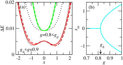
Figure 3: (Color online) (a) Effective oscillator potential for LM. Semi-classical estimate (dotted); SG estimate for $\zeta=0$ (full) and $\zeta=0.01$ (dashed). Parameters $\Omega=0.1$, $\Gamma=0.02$ and $U=0.3$ (for SG only) are in units of $D$ (half-width of the band). (b) The minima of the potential in semi-classical estimate.

We now turn to the renormalization of the vibrational mode and demonstrate that through the electron-phonon coupling the confining potential is diminished and can even be driven to the form of a double well. We first discuss $U=0$ model and use the semi-classical approximation in which phonon operators are substituted, $a\sim a^{\dagger}\to x/2$, by a real valued constant $x$. The resulting Hamiltonian with the hybridization $\tilde{\Gamma}(x)=\Gamma(1+g^{2}x^{2})$ is noninteracting and can be thus solved exactly. Here the magnitude of the bare hybridization with $g=0$ is defined by $\Gamma=\pi V^{2}/D$. In this model only the hybridization energy gain, which in the wide-band limit ($\Gamma/D$ small) readsFabrizio (2007) $\Delta E_{\mathrm{hyb}}=-2/\pi\tilde{\Gamma}\log D/\tilde{\Gamma}$, and the elastic energy cost $\Delta E_{\mathrm{el}}=\Omega x^{2}/4$ are a function of $x$. Hence, the effective oscillator potential in this estimate is $\Delta E_{\mathrm{SC}}=\Delta E_{\mathrm{el}}+\Delta E_{\mathrm{hyb}}$ and can be written in a closed form

$$\Delta E_{\mathrm{SC}}(x)=\Omega x^{2}/4-(2/\pi)\tilde{\Gamma}(x)\log\{D/[\tilde{\Gamma}(x)]\}.$$ (20)

The prefactor of the $x^{2}$-term in the small-$x$ expansion is equal to $\Omega/4-\left\{(2/\pi)g^{2}\Gamma\left[\log(D/\Gamma)-1\right]\right\}$ and is decreasing with increasing $g$ indicating the softening of the confining potential. At sufficiently large $g$, two wells emerge. In Fig. 3 (a) we plot (dotted) the resulting potential for $g$ below and above the delimiting value ($g_{\mathrm{d}}$). The $g_{\mathrm{d}}$ and the positions $x_{\mathrm{m}}$ [shown in Fig. 3(b)] of the potential minima can be extracted analytically from Eq. (20),

$$g_{\mathrm{d}} = \sqrt{\frac{\pi\Omega}{8\Gamma\left[\log(D/\Gamma)-1\right]}},$$ (21)

$$x_{\mathrm{m}} = \sqrt{\frac{\pi\Omega(g-g_{\mathrm{d}})}{4\Gamma g_{\mathrm{d}}^{5}}}.$$ (22)

For a finite $U$ the model cannot be solved exactly, but by estimating the potential with the SG method, we find that the evolution of the potential as just described persists. The SG results for $U>0$ are plotted in Fig. 3 for $\zeta=0$ (full lines) and also for the case with broken left-right symmetry $\zeta=0.01$ (dashed). While for $g<g_{\mathrm{d}}$ the potential is only slightly perturbed, finite $\zeta$ for $g>g_{\mathrm{d}}$ breaks the degeneracy between the two minima. In this regime, the molecule is attracted to one of the electrodes.

Having defined the characteristic values $g_{\mathrm{c}}$ and $g_{\mathrm{d}}$ it is interesting to ask whether there is any relation between the two. As discussed above, the 2CK point occurs at $g_{\mathrm{c}}$ such that in the semi-classical description $1-g_{\mathrm{c}}|x|\sim 0$, meaning that the double well-potential has to be preformed for its minima to occur at $|x_{\mathrm{m}}|\gtrsim 1/g_{\mathrm{c}}$. Therefore we expect $g_{\mathrm{c}}>g_{\mathrm{d}}$. However, as $x_{\mathrm{m}}$ evolves rapidly as a function of $g$ the values of $g_{\mathrm{c}}$ and $g_{\mathrm{d}}$ are close.

To support this statements quantitatively in Table 1 we show the semi-classical (SC) and SG estimates of $g_{\mathrm{d}}$ compared to the SW and NRG estimates of $g_{\mathrm{c}}$ for several values of parameters. As expected, we find that the Schrieffer-Wolff estimate of $g_{\mathrm{c}}$ becomes more accurate (agrees better with the NRG) for $U,\Omega$ large when the charge fluctuations and phonon excitations are suppressed. Conversely, the semi-classical estimate is more accurate for large number of excited phonons (small $\Omega$) and small $U$ but breaks down for large $U$. For example, for $\Omega=1$ and $U=3$ the value obtained by the semi-classical method overestimates $g_{\mathrm{d}}$ to a value which is larger than $g_{\mathrm{c}}$ obtained using NRG.

Table 1: SC and SG: $g_{\mathrm{d}}$ obtained from semi-classical (SC) estimate and from SG simulations. SW and NRG: $g_{\mathrm{c}}$ calculated by SW estimates and from NRG simulations. SG method is inapplicable for very large $U$.

$\Omega$	$U$	SC	SG	SW	NRG
0.1	0.3	0.82	0.85	1.29	0.84
0.1	0.6	0.82	/	1.15	0.85
1	0.03	2.60	2.59	8.22	3.11
1	0.3	2.60	2.32	2.76	2.32
1	3	2.60	/	1.29	1.28

IV.2 Exponential modulation

Let us perform the Schrieffer-Wolff transformation also on the model with exponential modulation of tunneling. We obtain

$$J_{e,o}=2V^{2}\sum_{m=0}^{\infty}\left(\frac{\delta_{m}^{e,o}}{-\epsilon+m\Omega}+\frac{\delta_{m}^{e,o}}{\epsilon+U+m\Omega}\right)$$ (23)

where $\delta_{m}^{e}=|\langle 0|\cosh(gx)|m\rangle|^{2}$ and $\delta_{m}^{o}=|\langle 0|\sinh(gx)|m\rangle|^{2}$. Note that as $J_{e}>J_{o}$ for all values of parameters no 2CK fixed point occurs in such a model. Note also that both $J_{\alpha}$ depend on $g$ exponentially. The Kondo temperature, which itself is exponential in $J$, $T_{K}\propto\exp(-1/\rho J)$, is thus very sensitive to the value of $g$.

The effective potential which is unbounded from below for $L\to\infty$ is regularized by the phonon cutoff $L$. At fixed $L$ we define $g_{\mathrm{e}}(L)$ as the value of $g$ at which the molecule is attracted by the hard wall boundary as signaled by an abrupt increase of displacement (shown later). Given $L$, the behavior of the model for $g>g_{\mathrm{e}}(L)$ becomes dominated by the hard-wall boundary only. For instance, the full curve in Fig. 2(b) corresponds to a particular $g$ which is smaller than $g_{\mathrm{e}}$ for the smaller phonon cutoff (dotted region) and larger than $g_{\mathrm{e}}$ for the larger phonon cutoff (dashed region). For $L\to\infty$, $g_{\mathrm{e}}\to 0$.

V Numerical results

In this section we confirm the anticipations stated above with numerical examples. We first show the results for LM and then for EM. We treat separately the inversion symmetric $\zeta=0$ and asymmetric $\zeta>0$ cases. We use the half-width of the band $D$ as the energy unit. Unless where explicitly stated, we take $U=0.3$, $\Gamma=\pi V^{2}/D=0.02$, and $\Omega=0.1$. All the results correspond to the particle-hole symmetric point, $\epsilon=-U/2$, and to the zero temperature limit.

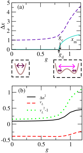
Figure 4: (Color online) (a) Fluctuations of displacement. (b) Fluctuations of charge, hopping to one of the electrodes and its fluctuations. The left (right) pictograms schematically present the effective oscillator potential before (after) the emergence of the soft mode ($U=0.3,\Gamma=0.02,\Omega=0.1$).

V.1 Linearized model

V.1.1 Inversion symmetry: $\zeta=0$

We begin by looking at the static quantities for $\zeta=0$. The average displacement $\langle x\rangle$ which is odd under inversion vanishes. The fluctuations of displacement $\Delta x=\langle(x-\langle x\rangle)^{2}\rangle^{1/2}$, shown in Fig. 4(a), increase monotonically with $g$. The slope of $\Delta x$ increases considerably at $g\sim g_{\mathrm{d}}$ $(\sim g_{\mathrm{c}})$, where the double well effective potential is formed, as indicated in pictograms. The change in slope is driven by the increased hybridization in the odd-channel. The position of the minima of effective potential $x_{\mathrm{m}}$ (full line) Eq. (22) also becomes non-vanishing there.

Due to increased hybridization the fluctuations of charge $\Delta n^{2}=\langle(n-1)^{2}\rangle$, shown in Fig. 4(b), are increased in the $g>g_{\mathrm{c}}$ regime. However, the absolute value of the average of the hybridization operator $v_{L}=\langle\widehat{v}_{L}\rangle=\langle\widehat{v}_{R}\rangle$ is diminished, contrary to the naive expectation. This is due to increasingly fluctuating sign of the overlap integral in this regime. On the other hand, the average of the hybridization operator squared $v_{L}^{2}=\langle\widehat{v}_{L}^{2}\rangle$ is increased here, as expected.

In Fig. 5 we plot the NRG flow diagram: the energies of the lowest few eigenstates in units of characteristic energy of a particular iteration $\omega_{N}\propto\Lambda^{-(N-1)/2}$ as the function of the NRG iteration number $N$. The fingerprint of the Fermi liquid ground state are the equidistant low-lying quasiparticle excitationsAffleck et al. (1992), which are seen for large $N$, irrespective of $g$. By comparing the top two panels with the bottom panel it is seen, that the roles of even and odd parity states are interchanged in the Fermi-liquid regime (right-hand side of each panel) corresponding to the change of the screening channel as $g$ is increased above $g_{\mathrm{c}}$.

For $g\sim g_{\mathrm{c}}$ (bottom panels) the unstable non-Fermi liquid fixed point, which determines the NRG flow at intermediate $N$ ($\sim 20$ for the plotted case) is discerned. The ratios of eigen-energies here (horizontal bars) are characteristic of the 2CK effect and agree with the predictions of conformal field theory Affleck et al. (1992) $(0,1/8,1/2,5/8,1,9/8,...)$. This regime cannot be explained in terms of the Fermi liquid quasiparticles. The difference between the couplings to the screening channels is a relevant perturbation and for low temperatures (large $N$) drives the flow towards the (stable) Fermi liquid fixed point.

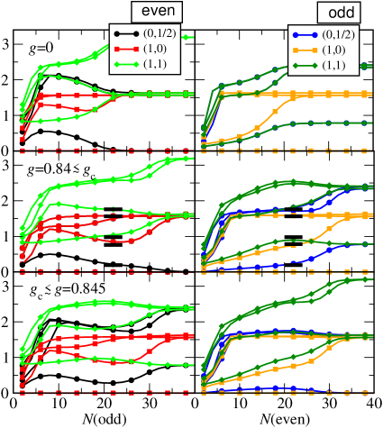
Figure 5: (Color online) NRG flow diagram. In the left (right) panels eigen-energies of states of even (odd) parity are shown for odd (even) number of NRG iterations, respectively. The states are labeled by ($Q$,$S$): total charge $Q$ and total spin $S$ quantum numbers. The thick horizontal bars are the conformal field theory predictions for 2CK fixed point. Parameters are as in Fig. 4.

Now we turn to the renormalization of the phonon propagator by the electron-phonon coupling. The dynamical information about oscillator is contained in the displacement Green’s function. The displacement spectral function

$$\mathcal{A}(\omega) =-\frac{1}{\pi}\mathrm{Im}\ll x,x\gg_{\omega}=$$

$$=-\frac{1}{\pi}\mathrm{Im}\int_{0}^{\infty}(-i)\langle[x(t),x(0)]\rangle e^{i\omega t}dt$$ (24)

is an odd function of $\omega$ due to the hermiticity of $x$ (unlike $\mathrm{Im}\ll a,a^{\dagger}\gg_{\omega}$ which is odd only for the inversion symmetric case $\zeta=0$). Since in NRG $\mathcal{A}(\omega)$ is evaluated for a finite system it consists of several $\delta$-peaks of different weights. To obtain a smooth spectral function we have used the Gaussian broadening on the logarithmic scaleBulla et al. (2001), where the Dirac $\delta$ function is broadened according to

$$\delta(\omega-\omega_{n})\to\frac{1}{b\omega_{n}\pi}\exp\left\{-\left[\frac{\log(\omega/\omega_{n})}{b}\right]^{2}-\frac{b^{2}}{4}\right\},$$ (25)

and we used $b=0.3$ in our calculations.

In Fig. 6(a) we plot $\mathcal{A}(\omega)$ for various $g$. The width of the high frequency peaks is overestimated (the extreme example is the $g=0$ peak at $\Omega$ for which the width should vanish) due to the broadening procedure described above. We could use Dyson equation Bulla et al. (1998); Jeon et al. (2003) to obtain sharper peaks but on one hand there is no a priori guarantee that such a procedure gives more accurate results for large $g$ and on the other hand we do not use the width of the peaks as a means to draw any quantitative conclusion.

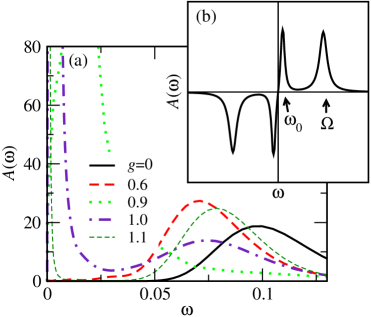
Figure 6: (Color online) (a) Displacement spectral functions for various $g$. Note the softening of the phonon mode. For large $g$ only small amount of spectral weight resides at low frequencies. The peaks at large frequencies appear broader than they should be because of the broadening procedure described in the text. Parameters are as in Fig. 4. (b) Spectral function after the emergence of the soft mode schematically. The frequencies of the soft mode $\omega_{0}$ and the high-frequency oscillation at $\omega\sim\Omega$ are indicated.

The evolution of the phonon operator can be understood in terms of the evolution of effective confining potential (Fig. 3, pictograms in Fig. 4). For intermediate $g$ [starting at $g\sim 0.5$ for the parameters used in Fig. 6(a)] as the confining potential starts to diminish the vibrational mode begins to soften: the peak of $\mathcal{A}(\omega)$ moves to lower frequencies. At still larger $g\sim g_{\mathrm{d}}$ two peaks emerge at the point where the two wells develop in the effective potential. Characteristic dependence of $\mathcal{A}(\omega)$ in this regime is schematically presented in Fig. 6(b). The double well potential is already well established and the major part of the spectral weight corresponds to the oscillations within each of the wells. The minor, low frequency part corresponds to increasingly slow tunneling (see also Fig. 8) between the degenerate minima of the potential. The frequency $\omega_{0}$ and the weight of the low frequency peak decrease with increasing $g$.

Due to the inversion symmetry the conductance can be calculated using the scattering phase shifts only, as described in Appendix C. The scattering phase shifts in the even and odd channels are $\pi/2(0)$ and $0(\pi/2)$, for $g<g_{\mathrm{c}}$ $(g>g_{\mathrm{c}})$ and the conductance evaluated by Eq. (54) is unity Mravlje et al. (2006).

V.1.2 Broken inversion symmetry: $\zeta>0$

It is impossible to experimentally produce perfectly symmetric devices, therefore it is interesting to check for the influence of the inversion symmetry breaking term of relative strength $\zeta$. Let us first remark that the NRG flow diagrams (not shown here) are that of the Fermi liquid as the occurrence of 2CK fixed point is inhibited by the breaking of inversion symmetry.

Figure 7: (Color online) Static quantities for system with broken inversion symmetry. (a) Averages of $x$, $x^{2}$, and $\Delta x$. (b) Averages of hopping $v_{L}$ and $v_{R}$ and fluctuations of charge. The breaking of inversion symmetry $\zeta=0.01$. Other parameters as in Fig. 4.

In Fig. 7 we plot static correlations for $\zeta=0.01$. New compared to the inversion symmetric case is the non-vanishing average displacement, which monotonically increases with $g$. Despite the simultaneous increase in average of $x^{2}$, the fluctuations of displacement $\Delta x=\langle(x-\langle x\rangle)^{2}\rangle^{1/2}$ eventually reach a maximum. At a still larger $g$ the molecule is attracted to the right electrode as indicated in the right pictogram. The fluctuations of charge are remain the same as in the $\zeta=0$ case but the average hopping to the right electrode $v_{R}$ is larger than $v_{L}$, which first vanishes and then changes sign. This asymmetry happens not at $g_{\mathrm{c}}\sim g_{\mathrm{d}}$ but at another value $g_{\mathrm{asy}}$ ($\sim 1$ for these parameters), when the softened phonon frequency $\omega_{0}$ and the energy difference between the hybridizations to left and right $\propto\zeta$ become comparable.

The spectral functions for $\zeta=0.01$ differ from the $\zeta=0$ case only for $g>g_{\mathrm{asy}}$. The distinction between the two cases is mainly that for $\zeta=0.01$ the frequency of the soft mode oscillation $\omega_{0}$ saturates. In Fig. 8, we plot the $\omega_{0}$ for both $\zeta$ as a function of $g$. For $\zeta=0.01$, we also plot the weight of the $\omega_{0}$ peak, which diminishes exponentially with increasing $g$.

Again, the behavior is easily understood in terms of the effective potential pictorially shown in Fig. 7. For small to intermediate $g$ the soft mode begins to emerge as the shape of the potential is transformed to a double-well-like form with the right well being lower in energy by a value $\Delta\propto\zeta$. When $g$ increases further and $\omega_{0}$ decreases below $\Delta$, the tunneling is suppressed. In this regime, the major part of the displacement spectral weight is due to the tunneling within the lower of the wells. The average displacement increases, its fluctuations decrease. Note that even a minor breaking of inversion symmetry results in a strongly asymmetric state through the mechanism described here.

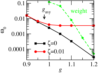
Figure 8: (Color online) The frequency (full lines) of the soft mode peak as a function of $g$. The weight of the soft mode peak for $\zeta=0.01$ and normalized to some arbitrary value (dashed). Other parameters are as in Fig. 4.

We plot also $\mathcal{A}(\omega)$ for different $\zeta$ and fixed $g=1.05>g_{\mathrm{asy}}$ in Fig. 9. The characteristic frequency of the soft mode is related to the energy-difference of the two wells and is proportional to $\zeta$ as shown in the inset of Fig. 9.

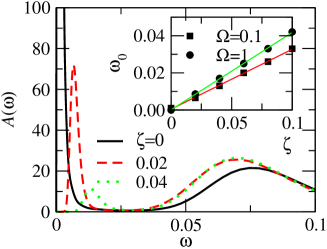
Figure 9: (Color online) (a) Displacement spectral functions for fixed $g=1.05$ and $\zeta=0,0.02,0.04$. Note the reduction of weight of low frequency peak on increasing $\zeta$. The high energy peak of $\zeta=0$ case is approached at still smaller $\zeta$. Inset: The position of low frequency peak as a function of $\zeta$ for $\Omega=0.1$, $g=1.05$ and $\Omega=1$, $g=7$. The full lines are fits to the data with slopes 0.32 and 0.42 for $\Omega=0.1,1$, respectively. Other parameters are as in Fig. 4.

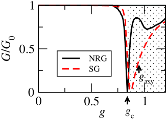
Figure 10: (Color online) Conductance as calculated from the current-current correlation function obtained by NRG (full) and from the SG method. The shaded region indicates the region the results are outside of the scope of the linearized model. $\zeta=0.01$, other parameters are as in Fig. 4.

The conductance for $\zeta>0$ cannot be obtained from the scattering phase shift alone since the rotation angle $\theta$ (see Appendix C) is not known in the present case of broken symmetry. Therefore we calculated the conductance from the current-current correlation function. We plot the conductance calculated by NRG and SG in Fig. 10. The conductance decreases to zero at $g\sim g_{\mathrm{c}}$. This minimum corresponds to the virtual decoupling of the left electrode, $1-gx\sim 0$, there on the average. Due to linearization, for still larger $g$ the magnitude of the overlap to the left electrode increases again. Correspondingly, the conductance is increased. The access to this region (denoted shaded) is probably unaccomplishable in measurements of transport through molecules.

The NRG and the SG data agree well for most $g$. However, for $g\sim g_{\mathrm{asy}}$ the maximum and minimum are seen in the NRG results, a feature which the effective Hamiltonian of the SG method fails to capture. The discrepancy is especially visible for the parameters used here for which $g_{\mathrm{c}}\sim g_{\mathrm{asy}}$ (compare also with data given in Appendix A). The NRG and SG for $g>g_{\mathrm{asy}}$ agree again. Here the fluctuations of displacement are diminished and the behavior is efficiently described in terms of the effective Hamiltonian with asymmetric coupling to the electrodes.

V.2 Exponential model

We now turn to the model with exponential modulation. Here even for the inversion symmetric model ($\zeta=0$) the 2CK Kondo fixed point is inaccessible because the coupling to the even channel is invariably stronger than the coupling to the odd channel. Correspondingly, the finite size spectra shown in Fig. 11(a) are that of the Fermi liquid ground state with the spin screened by the even conduction channel. Even at large $g$, the even and the odd channels do not inter-change their roles in the screening, confirming such an inter-change in the model with LM is indeed an artifact of the linearization.

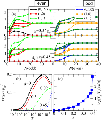
Figure 11: (Color online) Model with exponential modulation of overlap integrals (EM). $L=10$, other parameters as in Fig. 4. (a) NRG eigenvalues. (b) Impurity contribution to magnetic susceptibility. For $g>g_{\mathrm{e}}$ the local moment regime is absent. Diamonds indicate the susceptibility calculated using the Bethe ansatz. (c) The Kondo temperature.

In Figs. 11(b) we plot the impurity contribution to the magnetic susceptibility $\chi$. Dimensionless susceptibility $kT\chi/(2\mu_{B})^{2}$, where $k$ is the Boltzmann constant and $\mu_{B}$ the Bohr magneton, has a peak at intermediate temperatures corresponding to the local moment regime provided that $g$ is below some critical value $g_{\mathrm{e}}$. For $g>g_{\mathrm{e}}$ the local moment regime is absent. By fitting the Bethe ansatz results for $S=1/2$ Kondo impurity to the numerically calculated susceptibility, following the procedure described in Refs. Desgranges and Schotte, 1982; Rajan et al., 1982; Sacramento and Schlottmann, 1989, we obtain the estimate of the Kondo temperature $T_{K}$, shown in Fig. 11(c). $T_{K}$ is increasing rapidly near $g_{\mathrm{e}}$ as effective hybridization grows large. For $g>g_{\mathrm{e}}$ the Kondo temperature is not defined because there is no local moment in the system.

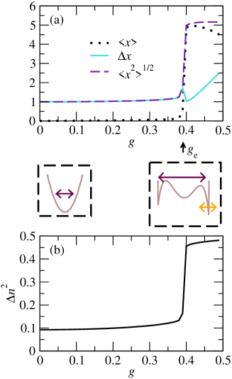
Figure 12: (Color online) (a) Average displacement and its fluctuations. (b) Fluctuations of charge. Phonon cutoff $L=10$, $\zeta=0.1$, other parameters as in Fig. 4.

In Fig. 12(a) we plot the averages of displacement and its fluctuations for $\zeta=0.1$. For $g>g_{\mathrm{e}}$, the displacement rises abruptly to the values that are limited only by the phonon cutoff; for $\zeta=0$ (not shown) the same applies to the fluctuations of displacement (displacement itself is zero). The abrupt increase is due to the increased hybridization, which is exponential in displacement. The gain in the kinetic energy cannot be compensated by the cost in oscillator potential, which is only quadratic in the displacement operators. In this regime, due to the exponentially increased hybridization, the fluctuations of charge, shown in Fig. 12(b), are near-maximal. The molecule resides in the effective potential presented in the right pictogram, which has the same form as the function plotted in Fig. 2(b) (dashed), and is attracted to the right electrode.

The value $g_{\mathrm{e}}$ can be estimated by first recognizing that the maximum $x$ is bounded by the phonon cutoff $L$: $x\lesssim x_{\mathrm{max}}=2\sqrt{L}$ and then solving $\Omega x_{\mathrm{max}}^{2}/4=V\exp(gx_{\mathrm{max}})$ for $g$, which gives

$$g_{\mathrm{e}}=\frac{1}{2\sqrt{L}}\log\left(\frac{\Omega}{V}L\right).$$ (26)

The comparison between this estimate and the numerical data is shown in Fig. 13. In the limit of large number of allowed phonons $L\to\infty$ critical value $g_{\mathrm{e}}\to 0$. An important result is that the model with exponential modulation of hybridization is not well-defined with quadratic stabilizing potential only as the results strongly depend on the cutoff.

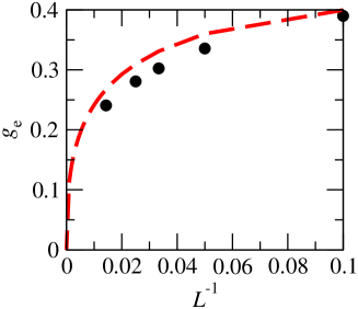
Figure 13: (Color online) Values $g_{\mathrm{e}}$ where the breakdown of the exponential model occurs for phonon cutoffs $L=10,20,30,40,70$ (circles). Other parameters are as in Fig. 4. Semi-classical estimate of $g_{\mathrm{e}}$ (dashed).

In Fig. 14 we plot the spectral function $\mathcal{A}(\omega)$. With increasing $g\lesssim g_{\mathrm{e}}$ the bare oscillator peak starts to soften. At $g>g_{\mathrm{e}}$ the molecule is attracted next to the hard wall boundary and remains mainly trapped into one of the wells defined by the phonon-cutoff. The high-frequency part of the spectral function in Fig. 14 corresponds to the oscillations within these wells. The wells are strongly anharmonic which is reflected in the broad distribution of spectral weight. The low frequency part of the spectral weight is due to the oscillations between the wells.

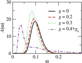
Figure 14: (Color online) Spectral functions exponential modulation. $\zeta=0.1$, $L=10$, other parameters as in Fig. 4.

A natural question which arises at this point is whether it is possible to tune the parameters so as to drive EM to the regime with developed double well potential, but for $g$ sufficiently lower than $g_{\mathrm{e}}$, so that the wells are not next to the hard wall boundary. For the parameter set used in the results shown, for example, this is not possible, because

$$g_{\mathrm{d}}>g_{\mathrm{e}}$$ (27)

for all $L$.

It can be shown that the inequality Eq. (27) holds in general. We begin by maximizing $g_{\mathrm{e}}$ with respect to $L$ (treating $L$ as if it was a continuous variable) and obtain

$$g^{\prime}_{\mathrm{e}}=\max_{L}g_{\mathrm{e}}(L)=\frac{\pi^{1/4}\sqrt{\Omega}}{e(D\Gamma)^{1/4}}.$$ (28)

The ratio between $g_{\mathrm{d}}$ defined in Eq. (21) and $g^{\prime}_{\mathrm{e}}$ can now be evaluated. We obtain that $g_{\mathrm{d}}/g^{\prime}_{\mathrm{e}}\geq(e^{7}\pi)^{1/4}/4\sim 1.92$. The double well potential thus develops also in EM but the wells are near the boundary defined by the phonon cutoff.

V.3 Regularized exponential model

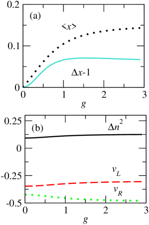
Figure 15: (Color online) Results for a model with overlap integrals modulated as $V_{L,R}(x)\sim\exp(\mp gx)/\cosh(gx)$, Eq. (29), with $\zeta=0.1$ and other parameters as in Fig. 4. (a) Displacement and its fluctuations. (b) Expectation values of hoppings and fluctuations of charge.

By using EM some of the nonphysical results found in the model with LM are eliminated but others, such as the dependence on a cutoff parameter $L$, are introduced. Another possibility is to regularize EM,

$$V_{L,R}(x)=V\left[\exp(\mp gx)/\cosh(gx)\mp\zeta\right],$$ (29)

or in the symmetrized basis

$$V_{e}=\sqrt{2}V,\>\>V_{o}=\sqrt{2}V\left[\tanh(gx)+\zeta\right].$$ (30)

The inequality Eq. (9) is satisfied and the normalization with the cosh function ensures the model behaves well for large $x$.

For this model we evaluated the matrix elements of the Hamiltonian $\langle m|H|n\rangle$ ($|m\rangle,|n\rangle$ correspond to states with $m,n$ excited phonons) in the real space by reintroducing the Hermite polynomials, which is numerically more stable than the expansion of $\tanh(gx)$ in the power series in $x$. This procedure can be used for any form of modulation. For EM the procedure can be simplified because it is possible to evaluate $\langle m|\exp(gx)|n\rangle$ analytically via the Baker-Hausdorff equality.

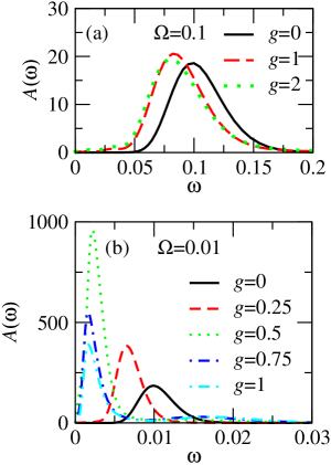
Figure 16: (Color online) (a) Displacement spectral functions for standard parameters as in Fig. 15. (b) Spectral functions for the same set of parameters, except for softer spring constant $\Omega=0.01$ and $\zeta=0.01$.

We first present results for parameters kept as in LM, Fig. 4, and with asymmetry parameter $\zeta=0.1$. Due to weaker dependence of the overlap integrals on displacement the effects of the electron-phonon coupling in this model are less pronounced. The displacement and its fluctuations, which we plot in Fig. 15(a) are small. This is accompanied by only a minor softening of the phonon mode, as shown in Fig. 16(a). The fluctuations of the charge and the expectation values of hopping, plotted in Fig. 15(b) are likewise only minorly distorted from the $g=0$ case. Note that we used $\zeta=0.1$ here, therefore the hoppings toward left and right electrodes differ considerably already for the $g=0$ case, a feature which is only slightly (compared to LM and EM) amplified by the dependence of the overlap integrals on $x$ for $g>0$. The reason for this moderate dependence of quantities on $g$ is the fact that the largest energy the system can gain by increasing the displacement is of the order of $V\propto\sqrt{\Gamma}$, which is for these parameters comparable to the elastic energy $\Omega x^{2}$ already for the displacements of order 1.

For smaller $\Omega=0.01$, i.e., a softer ’spring’, the effect of the electron-phonon coupling is larger and the soft mode is clearly developed, Fig. 16(b). Simultaneously other quantities ($\langle x\rangle$, $\Delta x$, etc.) also exhibit more pronounced behavior, similar to LM and EM cases (not shown here).

The regularized form, Eq. 29, might describe well the modulation of overlap integrals in realistic case and we believe that the softening of the phonon mode and related tendency toward broken symmetry configuration is the universal consequence of displacement-modulated hybridization.

VI Conclusion

In summary, we analyzed the influence of the electron-phonon coupling in molecular bridges consisting of a molecule oscillating between two electrodes. The overlaps between the molecular orbital and the orbitals in the electrodes are determined by the position of the molecule $x$. To model this situation we used several types of the dependence of the overlap integrals on $x$.

We find that the inversion symmetric model with linear modulation has a 2CK critical point at some critical electron-phonon coupling $g=g_{\mathrm{c}}$ where both channels participate equally to the screening of the spin. The occurrence of this critical point is suppressed if a finite difference $\zeta$ between the coupling to left and right electrodes is introduced. In such broken symmetry system the sharp transition between the two Fermi liquid states via a non Fermi liquid state is replaced by a continuous rotation of the screening state in the channel space from an almost symmetric to an almost antisymmetric linear combination of the left and right states. This continuous rotation is accompanied by a dip in conductance near the point where one of the electrodes is decoupled.

Additionally we found that the electron-phonon coupling modifies the shape of the effective potential affecting the static and dynamic properties of the oscillator. At moderate $g$ the potential is softened and the frequency of oscillations decreases. At large $g$ the potential develops side-wells and the phonon propagator consists of a part corresponding to high frequency oscillations within the well and another part corresponding to slow tunneling between the degenerate wells.

For finite $\zeta$ the degeneracy between the wells is broken by an amount $\propto\zeta$ and when the softened frequency $\omega_{0}$ drops below this value, the tunneling to the higher well is suppressed. In this regime, the average displacement starts to increase significantly and its fluctuations decrease. Hence, only a minor ($\sim\omega_{0}$) breaking of inversion symmetry can result in a significantly asymmetric configuration, which could also account for the asymmetric configurations typically observed in some experiments.

We consider also overlap integrals exponentially modulated by the displacement, which is closer to reality in the respect that the coupling to the even channel is invariably stronger. However, due to the exponential increase in hybridization energy gain, this model is not stable against large distortions. The value of $g$ at which this instability starts is set by the phonon cutoff and vanishes in the limit of large cutoff. We analyzed the model at finite cutoff and found that the 2CK fixed point is absent, but the other behavior of the LM is qualitatively recovered. In particular, the softening occurs with increasing $g$ and for large $g$ the molecule is attracted to one of the electrodes and is localized next to the boundary given by the phonon cutoff. In this regime, the Kondo temperature is significantly increased but the conductance is suppressed due to the small overlap with one of the electrodes.

The main common finding is thus the softening of the phonon mode, emerging for linearized and exponential modulations, as well as for the case of a more realistic regularized modulation. If the inversion symmetry is broken, the instability due to the formation of a double well effective potential will manifest as the attraction of the molecule into one of the wells and simultaneous suppression of the conductance. The instability inspired also a very recent work, in which the break-junctions are studied as an example of a two-level systemLucignano et al. (2008).

Finally, let us comment on the relevance of the presented work outside the scope of the experiments with molecular conductors. Within the dynamical mean field theory (DMFT) Georges et al. (1996) the bulk correlated electron systems are solved by mapping onto impurity problems. Likewise, bulk systems with electron-phonon coupling are mapped onto impurity (or impurity-cluster) problems with coupling to phonons. In this regard the knowledge of the behavior of the impurity problems is a convenient guide in the interpretation of the DMFT results. The results obtained in this work for the linearized model correspond to the general two-band case, where the coupling to one of the bands is phonon-assisted. The large $g$ regime which we dismissed as unphysical could prove relevant in this context.

Our results could also be applied to the studies of nanoelectromechanical systems Gorelik et al. (1998); Craighead (2000); Cleland et al. (2002); Flowers-Jacobs et al. (2007); Doiron et al. (2008) (NEMS). In NEMS the tunneling to electrodes is modulated by the displacement of the cantilever in a similar fashion as analyzed in this work. Once the dimensions of these devices are reduced to such an extent that the frequencies of the oscillations will become comparable to other scales, such as the bias at which the devices are operated, softening of the vibrational mode and susceptibility towards large displacements could be observed. For instance, we predict that the frequency of the oscillations will decrease if the tunneling rate from the electrodes to the perpendicularly situated cantilever immersed between them is increased.

Appendix A Comparison to Schönhammer-Gunnarsson projection-operator method

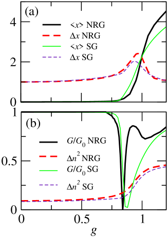
Figure 17: (Color online) Comparison between Shönhammer-Gunnarsson and NRG results. (a) Displacement and displacement fluctuations. (b) Conductance and charge fluctuations. $U=0.3$, $\Gamma=0.02$, $\Omega=0.1$, $\zeta=0.01$.

In this appendix we compare the results of NRG calculations to the results obtained by the SG method. Let us summarize first the results we have obtained using the SG method for model II of Refs. Mravlje et al., 2006, 2008. We have found that for $g$ large enough the variational solution with broken inversion symmetry is lower in energy. This occurs even for $\zeta=0$ when the inversion symmetry should persist. That indicates that for large $g$ due to the instability in the system the SG method fails giving a solution with ’spontaneously’ broken symmetry. Such failure is typical of the mean-field treatment. However, from our previous analysisMravlje et al. (2006) it was not clear whether the failure occurs at the point where the symmetry of the screening channel is changed or at the point when the soft mode is formed (or the two phenomena occur simultaneously).

In Fig. 17 we compare the displacement, its fluctuations and the fluctuations of charge calculated by SG method to the NRG results. They match closely, with the exception of discrepancies in the precise values of increased displacement fluctuations and range of $g$ where these occur. Conductance is discussed in the main text, here we re-plot the curve for completeness.

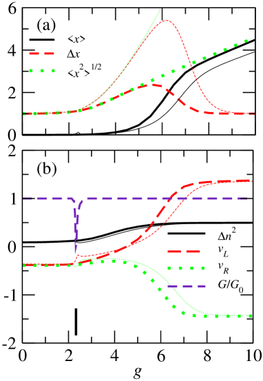
Figure 18: (Color online) $\Omega=1$, other data as in Fig. 17. Thick lines: NRG, thin lines: SG; (a) Expectation values of $x$ and its fluctuations. (b) Fluctuations of occupancy and expectation values of hoppings to left and right electrodes. The vertical lines denote $g_{\mathrm{c}}$ (thick) and the value of $g$ where the minimum of conductance calculated by SG method occurs (dotted). Conductance curves (dashed) obtained by NRG and SG coincide.

In Fig. 18(a) we show the results for $\Omega=1$ where the discrepancy between NRG results (thick) and SG results (thin) is larger. In this regime SG method overestimates the value of displacement and its fluctuations. More interestingly, in Fig. 18(b) the jump in expectation values of hopping operators and a minimum in the conductance are seen in the variational results near the value $g_{\mathrm{c}}\sim 2.3$. Here also a small peak in displacement is seen.

If $\zeta=0$ there is no ’spontaneous’ symmetry breaking in SG method for this $\Omega$. By combining these results we conclude that the appearance of asymmetric solution in SG will coincide with the change in the symmetry of the screening channel from even to odd, but only when the soft mode is sufficiently developed, otherwise only a finite jump in $v_{L}$, $v_{R}$ occurs there.

Let us remark here also that in terms of the effective Hamiltonian, the $g<g_{\mathrm{c}}(g>g_{\mathrm{c}})$ regimes correspond to the state, where the hopping to left and right electrodes has equal and opposite phases, respectively. The non-Fermi liquid $g=g_{c}$ regime cannot be described in terms of (Fermi-liquid) effective Hamiltonian. Nevertheless, insisting upon this description, it can be regarded as a combination of states which correspond to two effective Hamiltonians in which left and right electrodes are, respectively, decoupled.

Appendix B Schrieffer-Wolff transformation

To obtain the effective-low energy Hamiltonian $H_{\mathrm{eff}}$ we first divide the Hamiltonian into two partsColeman (2002)

$$H=H_{0}+\lambda H^{\prime}$$ (31)

where $H_{0}$, which for our example reads

$$H_{0}=\epsilon n+Un_{\uparrow}n_{\downarrow}+\Omega a^{\dagger}a+H_{L}+H_{R},$$ (32)

is diagonal in the low ($n=1$, no excited phonons) and high ($n=2,0$, with excited phonons) energy subspaces (for $\epsilon\sim-U/2$, $U$ and $\Omega$ large). The hybridization part

$$H^{\prime}=V\widehat{v}_{e}+Vgx\widehat{v}_{o}$$ (33)

provides the mixing between the low and high energy subspaces and $\lambda$ serves as an expansion parameter to be set to $1$ at the end of the derivation.

Then a canonical transformation generated by some unitary operator $e^{\cal S}$ is performed to obtain the block-diagonal

$$\tilde{H}=e^{{\cal S}}He^{-{\cal S}}=\begin{pmatrix}H_{L}&0\\ 0&H_{H}\end{pmatrix}.$$ (34)

By expanding Eq. (34) in terms of nested commutators $\tilde{H}=H+[{\cal S},H]+[{\cal S},[{\cal S},H]]/2+...$ and the generator ${\cal S}$ as a power-series in $\lambda$, ${\cal S}={\cal S}_{1}\lambda+{\cal S}_{2}\lambda^{2}+...$, to second order in $\lambda$ the following should hold:

$$\tilde{H}=H_{0} +\lambda(H^{\prime}+[{\cal S}_{1},H_{0}])+$$ (35)

$$+\lambda^{2}([{\cal S}_{1},H^{\prime}]+\frac{1}{2}[{\cal S}_{1},[{\cal S}_{1},H_{0}]]+[{\cal S}_{2},H_{0}]).$$

Relation Eq. (35) is satisfied to lowest order in $\lambda$ by demanding

$$H^{\prime}+[{\cal S}_{1},H_{0}]=0.$$ (36)

Since ${\cal S}_{1}$ can be chosen completely block-off-diagonal the commutator $[{\cal S}_{1},H^{\prime}]$ is block-diagonal, therefore Eq. (34) is satisfied also to second order in $\lambda$ by taking ${\cal S}_{2}=0$. Looking now at the matrix element of Eq. (36) in the basis of eigenstates of $H_{0}$ (we will use Latin indices for states in low-energy subspace, and Greek indices for states in high-energy subspace), we obtain ${\cal S}_{\alpha b}=H^{\prime}_{\alpha b}/(E_{\alpha}-E_{b})$.

Finally, the high energy part is neglected by projecting to the low energy subspace

$$H_{\mathrm{eff}}=P_{\mathrm{low}}H_{0}P_{\mathrm{low}}+H^{\mathrm{I}}_{\mathrm{eff}}$$ (37)

with the projector

$$P_{\mathrm{low}}=|0\rangle\langle 0\rangle\left[n_{\uparrow}(1-n_{\downarrow})+n_{\downarrow}(1-n_{\uparrow})\right]$$ (38)

where $|m\rangle$ denotes normalized phonon state with $m$ excited phonons and the effective interaction $H^{\mathrm{I}}_{\mathrm{eff}}$ is due to the virtual transitions to the high energy states. Its matrix elements read

$$H_{\mathrm{eff};ab}^{\mathrm{I}}=\frac{1}{2}\sum_{\gamma\in\mathrm{high}}\left(\frac{H^{\prime\dagger}_{a\gamma}H^{\prime}_{\gamma b}}{E_{a}-E_{\gamma}}+\frac{H^{\prime\dagger}_{a\gamma}H^{\prime}_{\gamma b}}{E_{b}-E_{\gamma}}\right).$$ (39)

In this case the Hamiltonian can be up to a constant term recast by using the spin operators to the form of the 2CK model

$$H_{\mathrm{eff}}^{\mathrm{I}}=H_{\mathrm{2CK}}=J_{e}\mathbf{S}\cdot\mathbf{s}_{e}+J_{o}\mathbf{S}\cdot\mathbf{s}_{o},$$ (40)

where the $s_{\alpha}$ for $\alpha=e,o$ denote the spin densities which read

$$\mathbf{S}=\frac{1}{2}\sum_{ss^{\prime}}d^{\dagger}_{s}\boldsymbol{\sigma}_{ss^{\prime}}d_{s^{\prime}}$$ (41)

for $d$-orbital and likewise for orbitals $\alpha$. Here the components of $\boldsymbol{\sigma}$ are the Pauli matrices. The coupling constant to the even channel is

$$J_{e}=2V^{2}\left(\frac{1}{-{\epsilon}}+\frac{1}{{\epsilon}+U}\right).$$ (42)

For the odd channel we get

$$J_{o}=2V^{2}g^{2}\left(\frac{1}{-\epsilon+\Omega}+\frac{1}{\epsilon+U+\Omega}\right),$$ (43)

where the $\Omega$ in the denominators occur since high-energy states involve one excited phonon.

For the exponential modulation the hybridization parts read

$$H^{\prime}_{e}= V\cosh(gx)v_{e},$$ (44)

$$H^{\prime}_{o}= V\sinh(gx)v_{o}.$$

The low-energy Hamiltonian is again that of the 2CK model and the coupling constants read

$$J_{e}=2V_{s}^{2}\sum_{m=0}^{\infty}\left(\frac{\delta_{m}^{e}}{-\epsilon+m\Omega}+\frac{\delta_{m}^{e}}{\epsilon+U+m\Omega}\right),$$ (45)

$$J_{o}=2V_{s}^{2}\sum_{m=0}^{\infty}\left(\frac{\delta_{m}^{o}}{-\epsilon+m\Omega}+\frac{\delta_{m}^{o}}{\epsilon+U+m\Omega}\right),$$ (46)

where $\delta_{m}^{e,o}=|\langle 0|(e^{gx}\pm e^{-gx})/2|m\rangle|^{2}=\exp(g^{2})g^{2m}/m!$ for $m$ even (odd) and zero otherwise, respectively.

Appendix C Conductance

The linear response conductance for a general interacting system is given by the Kubo formulaIzumida et al. (1997)

$$G=\lim_{\omega\to 0}\frac{e^{2}}{\omega}\mathrm{Im}C_{II}^{R}(\omega),$$ (47)

where

$$C_{II}^{R}(\omega)=-i\lim_{\eta\to 0}\int_{0}^{\infty}[I(t),I(0)]e^{i(\omega+i\eta)t}dt$$ (48)

is the retarded current-current correlation function and the current operators are defined by the time derivative of the electrons in the electrodes

$$I=\frac{\dot{N}_{R}-\dot{N}_{L}}{2}.$$ (49)

For Fermi liquid systems at $T=0$ the current-current correlation function can be expressed in terms of the Green’s function $G_{nn^{\prime}}(\omega)$ involving sites $n,n^{\prime}$ in the electrodes. The conductance is then given by the Landauer formula (Fisher-Lee relationFisher and Lee (1981))

$$G=G_{0}|t(0)|^{2},$$ (50)

where $G_{0}=2e^{2}/h$ is the quantum of conductance and the transmission amplitude $t(\omega)$ can be written asOguri (1997, 2001)

$$t(\omega)=\frac{1}{-i\pi\rho(\omega)}e^{-ik(n-n^{\prime})}G_{n^{\prime}n}(\omega+i\eta).$$ (51)

Alternatively, the transmission amplitude can be expressed also in terms of the scattering matrix $S_{\alpha\alpha^{\prime}}$ which relates the amplitudes of the outgoing wave in electrode $\alpha$ to the amplitude of the incoming wave in the electrode $\alpha^{\prime}$

$$S=\begin{pmatrix}r_{L}&t_{R}\\ t_{L}&r_{R}\end{pmatrix},$$ (52)

where $r_{\alpha}$ ($t_{\alpha}$) are the respective reflection and transmission coefficients. The scattering matrix can be rotated in the L-R space to the basis of channels (linear combinations of left and right states) where it is diagonalPustilnik and Glazman (2001)

$$USU^{-1}=\begin{pmatrix}e^{i2\delta_{a}}&0\\ 0&e^{i2\delta_{b}}\end{pmatrix},$$ (53)

where $U=\exp(i\theta\tau_{y})\exp(i\alpha\tau_{z})$ and $\tau_{i}$ are the Pauli matrices. According to the Landauer formula Eq. (50) the zero-temperature conductance is determined by the transmission probability $t(0)=S_{RL}=t_{L}$, hence we obtain

$$G/G_{0}=\sin^{2}(\delta_{a}-\delta_{b})\sin^{2}(2\theta).$$ (54)

The angle $\theta$ determines the maximal value of conductance. In the inversion symmetric case $\theta=\pi/4$, the phase-shifts $\delta_{\alpha}$ which occur in the even and odd channels can then be extracted from the NRG finite-size spectraOliveira and Wilkins (1981).

When the system is not inversion symmetric it is not possible to extract $\theta$ since the channel indices are not tracked. To evaluate the conductance in this case we resort to equation Eq. (47). The current operator $I=(\dot{N}_{L}-\dot{N}_{R})/2$ is obtained by commuting $N_{\alpha}=\sum_{k\sigma}n_{k\alpha\sigma}$ with the Hamiltonian for $\alpha=L,R$ and reads

$$\dot{N}_{L(R)}=-\frac{i}{\hbar}V_{L(R)}(x)\sum_{\sigma}(c_{1L(R)\sigma}^{\dagger}d-h.c.),$$ (55)

where $c_{1L(R)\sigma}^{\dagger}$ creates an electron in the orbital next to impurity in the left(right) electrode, respectively.

Alternatively, the conductance can be calculated also from the dependence of the ground state energy on auxiliary magnetic fluxMeden and Schollwöck (2003); Molina et al. (2003); Rejec and Ramšak (2003b, a) which is obtained by embedding the interacting system into auxiliary noninteracting ring and threading the ring with magnetic flux $\Phi$. Then the conductance can be expressed asRejec and Ramšak (2003b, a)

$$G/G_{0}=\sin^{2}\left[\frac{\pi}{2}\frac{E(\pi)-E(0)}{\Delta}\right],$$ (56)

where $E(\Phi)$ is the ground state energy of the auxiliary ring with embedded interacting system and $\Delta=1/\left[\rho(\epsilon_{F})N\right]$ the level spacing in the auxiliary ring with the density of states at the Fermi energy $\rho(\epsilon_{F})$ which consists of $N$ sites. This approach is useful especially in connection to variational approaches [such as SG, although in SG we can extract the conductance also from Eq. (50) directly and obtain same results], where the ground state energy is the most reliable quantity.

References

- Goldhaber-Gordon et al. (1998) D. Goldhaber-Gordon, H. Shtrikman, D. Mahalu, D. Abusch-Magder, U. Meirav, and M. A. Kastner, Nature 391, 156 (1998).
- Madhavan et al. (1998) V. Madhavan, W. Chen, T. Jamneala, M. F. Crommie, and N. S. Wingreen, Science 280, 567 (1998).
- Liang et al. (2002) W. Liang, M. P. Shores, M. Bockrath, J. R. Long, and H. Park, Nature 417, 725 (2002).
- Park et al. (2002) J. Park, A. N. Pasupathy, J. I.Goldsmith, C. Chang, Y. Yaish, J. R. Petta, M. Rinkoski, J. P. Sethna, H. D. Abrunas, P. L. McEuen, et al., Nature 417, 722 (2002).
- Yu and Natelson (2004) L. H. Yu and D. Natelson, Nano Lett. 4, 79 (2004).
- Pasupathy et al. (2005) A. N. Pasupathy, J. Park, C. Chang, A. V. Soldatov, S. Lebedkin, R. C. Bialczak, J. E. Grose, L. A. K. Donev, J. P. Sethna, D. C. Ralph, et al., Nano Lett. 5, 203 (2005).
- Zhao et al. (2005) A. Zhao, Q. Li, L. Chen, H. Xiang, W. Wang, S. Pan, B. Wang, X. Xiao, J. Yang, J. G. Hou, et al., Science 309, 1542 (2005).
- Yu et al. (2005) L. H. Yu, Z. K. Keane, J. W. Ciszek, L. Cheng, J. M. Tour, T. Baruah, M. R. Pederson, and D. Natelson, Phys. Rev. Lett. 95, 256803 (2005).
- Balseiro et al. (2006) C. A. Balseiro, P. S. Cornaglia, and D. R. Grempel, Phys. Rev. B 74, 235409 (2006).
- Nuñez Regueiro et al. (2007) M. D. Nuñez Regueiro, P. S. Cornaglia, G. Usaj, and C. A. Balseiro, Phys. Rev. B 76, 075425 (2007).
- Cornaglia et al. (2007) P. S. Cornaglia, G. Usaj, and C. A. Balseiro, Phys. Rev. B 76, 241403 (2007).
- Nitzan and Ratner (2003) A. Nitzan and M. A. Ratner, Science 300, 1384 (2003).
- Tao (2006) N. J. Tao, Nature Nanotech. 1, 173 (2006).
- Galperin et al. (2007) M. Galperin, M. A. Ratner, and A. Nitzan, J. Phys.: Condens. Matter. 19, 103201 (2007).
- Roch et al. (2008) N. Roch, S. Florens, V. Bouchiat, W. Werndorfer, and F. Balestro, Nature 453, 633 (2008).
- Barišić et al. (1970) S. Barišić, J. Labbé, and J. Friedel, Phys. Rev. Lett. 25, 919 (1970), the idea of modulation of tunneling by displacement is neither new nor applies only to mesoscopic systems, see, e.g.,.
- Nozières and Blandin (1980) P. Nozières and A. Blandin, J. Physique (France) 41, 193 (1980).
- Mravlje et al. (2008) J. Mravlje, A. Ramšak, and R. Žitko, Physica B 403, 1484 (2008).
- Hewson and Meyer (2002) A. C. Hewson and D. Meyer, J. Phys: Condens. Matter 14, 427 (2002).
- Mravlje et al. (2005) J. Mravlje, A. Ramšak, and T. Rejec, Phys. Rev. B 72, 121403(R) (2005).
- Mravlje et al. (2006) J. Mravlje, A. Ramšak, and T. Rejec, Phys. Rev. B 74, 205320 (2006).
- Novotný et al. (2004) T. Novotný, A. Donarini, C. Flindt, and A.-P. Jauho, Phys. Rev. Lett. 92, 248302 (2004).
- Twamley et al. (2006) J. Twamley, D. W. Utami, H.-S. Goan, and G. Milburn, New J. Phys. 8, 63 (2006).
- Johansson et al. (2008) J. R. Johansson, L. G. Mourokh, A. Y. Smirnov, and F. Nori, Phys. Rev. B 77, 035428 (2008).
- Koch et al. (2006) J. Koch, M. E. Raikh, and F. von Oppen, Phys. Rev. Lett. 96, 056803 (2006).
- Hwang et al. (2007) M.-J. Hwang, M.-S. Choi, and R. López, Phys. Rev. B 76, 165312 (2007).
- Kiselev et al. (2006) M. N. Kiselev, K. Kikoin, R. I. Shekhter, and V. M. Vinokur, Phys. Rev. B 74, 233403 (2006).
- Wilson (1975) K. G. Wilson, Rev. Mod. Phys. 47, 773 (1975).
- Bulla et al. (2008) R. Bulla, T. A. Costi, and T. Pruschke, Rev. Mod. Phys. 80, 395 (2008).
- Žitko and Bonča (2006) R. Žitko and J. Bonča, Phys. Rev. B 74, 045312 (2006).
- Schönhammer (1976) K. Schönhammer, Phys. Rev. B 13, 4336 (1976).
- Gunnarsson and Schönhammer (1985) O. Gunnarsson and K. Schönhammer, Phys. Rev. B 31, 4815 (1985).
- Rejec and Ramšak (2003a) T. Rejec and A. Ramšak, Phys. Rev. B 68, 035342 (2003a).
- Rejec and Ramšak (2003b) T. Rejec and A. Ramšak, Phys. Rev. B 68, 033306 (2003b).
- Fabrizio (2007) M. Fabrizio, Lectures on the physics of strongly correlated systems (AIP, 2007), chap. I, p. 3.
- Affleck et al. (1992) I. Affleck, A. W. W. Ludwig, H.-B. Pang, and D. L. Cox, Phys. Rev. B 45, 7918 (1992).
- Bulla et al. (2001) R. Bulla, T. A. Costi, and D. Vollhardt, Phys. Rev. B 64, 045103 (2001).
- Bulla et al. (1998) R. Bulla, A. C. Hewson, and T. Pruschke, J. Phys: Condens. Matter 10, 8365 (1998).
- Jeon et al. (2003) G. S. Jeon, T.-H. Park, and H.-Y. Choi, Phys. Rev. B 68, 045106 (2003).
- Desgranges and Schotte (1982) H.-U. Desgranges and K. D. Schotte, Phys. Lett. 91A, 240 (1982).
- Rajan et al. (1982) V. T. Rajan, J. H. Lowenstein, and N. Andrei, Phys. Rev. Lett. 49, 497 (1982).
- Sacramento and Schlottmann (1989) P. D. Sacramento and P. Schlottmann, Phys. Rev. B 40, 431 (1989).
- Lucignano et al. (2008) P. Lucignano, G. E. Santoro, M. Fabrizio, and E. Tosatti, Phys. Rev. B 78, 155418 (2008).
- Georges et al. (1996) A. Georges, G. Kotliar, W. Krauth, and M. J. Rozenberg, Rev. Mod. Phys. 68, 13 (1996).
- Gorelik et al. (1998) L. Y. Gorelik, A. Isacsson, M. V. Voinova, B. Kasemo, R. I. Shekhter, and M. Jonson, Phys. Rev. Lett. 80, 4526 (1998).
- Craighead (2000) H. G. Craighead, Science 290, 1532 (2000).
- Cleland et al. (2002) A. N. Cleland, J. S. Aldridge, D. C. Driscoll, and A. C. Gossard, Appl. Phys. Lett. 81, 1699 (2002).
- Flowers-Jacobs et al. (2007) N. E. Flowers-Jacobs, D. R. Schmidt, and K. W. Lehnert, Phys. Rev. Lett. 98, 096804 (2007).
- Doiron et al. (2008) C. B. Doiron, B. Trauzettel, and C. Bruder, Phys. Rev. Lett. 100, 027202 (2008).
- Coleman (2002) P. Coleman, Lectures on the physics of strongly correlated electron systems VI (American Institute of Physics, 2002), vol. 629, chap. 2, pp. 79–160.
- Izumida et al. (1997) W. Izumida, O. Sakai, and Y. Shimizu, J. Phys. Soc. Jpn. 66, 717 (1997).
- Fisher and Lee (1981) D. S. Fisher and P. A. Lee, Phys. Rev. B 23, 6851 (1981).
- Oguri (1997) A. Oguri, J. Phys. Soc. Jpn. 66, 1427 (1997).
- Oguri (2001) A. Oguri, J. Phys. Soc. Jpn. 70, 2666 (2001).
- Pustilnik and Glazman (2001) M. Pustilnik and L. I. Glazman, Phys. Rev. Lett. 87, 216601 (2001).
- Oliveira and Wilkins (1981) L. N. Oliveira and J. W. Wilkins, Phys. Rev. B 24, 4863 (1981).
- Meden and Schollwöck (2003) V. Meden and U. Schollwöck, Phys. Rev. B 67, 035106 (2003).
- Molina et al. (2003) R. A. Molina, D. Weinmann, R. A. Jalabert, G.-L. Ingold, and J.-L. Pichard, Phys. Rev. B 67, 235306 (2003).