Pressure-energy correlations in liquids. II. Analysis and consequences

Abstract

We present a detailed analysis and discuss consequences of the strong correlations of the configurational parts of pressure and energy in their equilibrium fluctuations at fixed volume reported for simulations of several liquids in the previous (companion) paper [arXiv:0807.0550]. The analysis concentrates specifically on the single-component Lennard-Jones system. We demonstrate that the potential may be replaced, at fixed volume, by an effective power-law, but not simply because only short distance encounters dominate the fluctuations. Indeed, contributions to the fluctuations are associated with the whole first peak of the radial distribution function, as we demonstrate by an eigenvector analysis of the spatially resolved covariance matrix. The reason the effective power-law works so well depends crucially on going beyond single-pair effects and on the constraint of fixed volume. In particular, a better approximation to the potential includes a linear term, which contributes to the mean values of potential energy and virial, but not to their fluctuations, for density fluctuations which conserve volume. We also study in considerable detail the zero temperature limit of the (classical) crystalline phase, where the correlation coefficient becomes very close, but not equal, to unity, in more than one dimension; in one dimension the limiting value is exactly unity. In the second half of the paper we consider four consequences of strong pressure-energy correlations: (1) analyzing experimental data for supercritical Argon we find 96% correlation; (2) we discuss the particular significance acquired by the correlations for viscous van der Waals liquids approaching the glass transition: For strongly correlating viscous liquids knowledge of just one of the eight frequency-dependent thermoviscoelastic response functions basically implies knowledge of them all; (3) we re-interpret aging simulations of ortho-terphenyl carried out by Mossa et al. in 2002, showing their conclusions follow from the strongly correlating property; and (4) we briefly discuss the presence of the correlations (after appropriate time-averaging) in model biomembranes, showing that significant correlations may be present even in quite complex systems.

I Introduction

In the companion paperBailey et al. (2008a) to this work, referred to as Paper I, we detailed the existence of a strong correlation between the configurational parts of pressure and energy in several model liquids. Recall that (instantaneous) pressure $p$ and energy $E$ have contributions both from particle momenta and positions:Allen and Tildesley (1987)

$$p =Nk_{B}T(\mathbf{p}_{1},\ldots,\mathbf{p}_{N})/V+W(\mathbf{r}_{1},\ldots,\mathbf{r}_{N})/V$$ (1)

$$E =K(\mathbf{p}_{1},\ldots,\mathbf{p}_{N})+U(\mathbf{r}_{1},\ldots,\mathbf{r}_{N}),$$ (2)

where $K$ and $U$ are the kinetic and potential energies, respectively, and $T(\mathbf{p}_{1},\ldots,\mathbf{p}_{N})$ is the “kinetic temperature”,Allen and Tildesley (1987) proportional to the kinetic energy per particle. The configurational contribution to pressure is the virial $W$, which for a translationally invariant potential energy function $U$ is definedAllen and Tildesley (1987) by

$$W=-\frac{1}{3}\sum_{i}\mathbf{r}_{i}\cdot\mathbf{\nabla}_{\mathbf{r}_{i}}U$$ (3)

where $\mathbf{r}_{i}$ is the position of the $i$th particle. Note that $W$ has dimension energy. In the case of a pair potential $U_{\textrm{pair}}=\sum_{i<j}v(r_{ij})$ the expression for the virial becomesAllen and Tildesley (1987)

$$W_{\textrm{pair}}=-\frac{1}{3}\sum_{i<j}r_{ij}v^{\prime}(r_{ij})=-\frac{1}{3}\sum_{i<j}w(r_{ij})$$ (4)

where $w(r)\equiv rv^{\prime}(r)$.

It is the correlation between $U$ and $W$ that we are interested in, quantified by the correlation coefficient

$$R=\frac{\langle\Delta W\Delta U\rangle}{\sqrt{\langle(\Delta W)^{2}\rangle}\sqrt{\langle(\Delta U)^{2}\rangle}}.$$ (5)

Paper I documented the correlation in many systems, showing that this is often quite strong, with correlation coefficient $R>0.9$, while in some other cases it was found to be weak or almost non-existent. The latter included in particular models with additional significant Coulombic interactions. The purpose of this paper is two-fold. First we give a comprehensive analysis of the source of the correlation in the simplest “strongly correlating” model liquid, the standard single-component Lennard-Jones (SCLJ) fluid. Paper I presented briefly an explanation in terms of an effective inverse power-law potential. Here we elaborate on that in greater detail, and go beyond it. Secondly we discuss a few observable consequences and applications of the strong correlations. These range from their measurement in a real system to applications to systems as diverse as supercooled liquids and biomembranes.

In section II we present a detailed analysis for the SCLJ case, first in terms of an effective inverse power-law with exponent $\sim 18$. This accounts for the correlation at the level of individual pair-encounters by assuming that only the repulsive part of the potential, corresponding to distances less than the minimum of the potential $r_{m}$, is relevant for fluctuations, and that this may be well approximated by an inverse power-law. The value 18 is significant since this explains the “slope” $\gamma$ defined as

$$\gamma\equiv\sqrt{\frac{\langle(\Delta W)^{2}\rangle}{\langle(\Delta U)^{2}\rangle}},$$ (6)

observed to be $\sim 6$ for Lennard-Jones systems (Paper I). The slope is exactly $n/3$ for a pure inverse power-law potential with exponent $n$, a case with perfect $W,U$ correlation (Paper I). Section II continues with a discussion of the SCLJ crystal, which is also strongly correlating. This would seem to invalidate the dominance of the repulsive part, since only presumably distances around and beyond the potential minimum are important, at least at low and moderate pressure. In this case the correlation can be explained only when summation over all pairs is taken into account, thus the correlation emerges as a collective effect. There is a connection between the slope obtained in this way and that given by the effective inverse power-law; in fact they are quite similar. The third subsection in section II gives a more systematic analysis of which regions dominate the fluctuations in the liquid phase, using an eigenvector decomposition of the spatially-resolved covariance matrix. This matrix represents the contributions to the (co-)variances of potential energy and virial from different pair separations. It is demonstrated that the region around the minimum of the potential plays a substantial role. The final subsection in section II provides a synthesis of the insights from the previous subsections, resulting in an “extended effective power-law approximation”, which includes a linear term. The main point is that a linear term in the pair potential will contribute to the mean values, but not to fluctuations, of $W$ and $U$, if the volume is constant.

In section III we discuss some consequences, starting by considering whether the instantaneous correlations can be related to a measurable quantity in the normal liquid state, and demonstrating this with data for supercritical Argon, finding a correlation coefficient of 0.96. Next we focus on consequences for highly viscous liquids, where time-scale separation implies that instantaneous correlation between virial and potential energy can be related to a correlation between the time-averaged pressure and energy. The third subsection discusses consequences for aging, while the fourth briefly discusses connections with recent work by Heimburg and Jackson on biomembranes.

Finally, section IV concludes with an outlook reflecting on the broader significance of strong correlation, and its implications for the understanding of liquids, particularly in the context of viscous liquids (which has been our main motivation throughout this work).

II Analysis

II.1 The effective inverse power law

In this section we consider the SCLJ system, in the hope that it is simple enough that a fairly complete understanding of the cause of strong correlations is possible. Recall that $R>0.9$ for a wide range of states (Paper I). In order to understand the numerology better we consider a generalized Lennard-Jones potential, denoted LJ(a,b) ($a>b$):

$$v_{LJ}^{a,b}(r)\propto(\sigma/r)^{a}-(\sigma/r)^{b},$$ (7)

although the standard LJ(12,6) case will be used for most examples. Starting from the idea that short distances dominate fluctuations and that the observed correlations are suggestive of a power-law interaction, we show that at a given density, the Lennard-Jones potential may be approximated by a single effective inverse power law over a range from a little less than $\sigma$ (where $v_{LJ}$ changes sign) to around $r_{m}$, the location of the potential minimum ($r_{m}=2^{1/6}\sigma$ for LJ(12,6)), covering an energy range of approximately $-\epsilon$ to $+2\epsilon$, where $\epsilon$ is the well-depth. At first sight, one might expect that if this were at all the case, the effective power would be less than $a$, somehow a mixture of the two exponents $a$ and $b$. It was noticed by Ben-Amotz and Stell,Ben-Amotz and Stell (2003) however, that the repulsive core of the LJ(12,6) potential may approximated by an inverse power law with an exponent $\sim$18, in agreement with our data (Paper I). To see how we get an exponent greater than $a$, note that the exponent $n$ in an inverse power law can be extracted from different ratios of derivatives:

$$v_{PL}(r)=Ar^{-n}+B,$$ (8)

where $B$ is a constant. This implies that

$$n =\frac{-rv_{PL}^{\prime}(r)}{(v_{PL}(r)-B)}$$

$$=\frac{-rv_{PL}^{\prime\prime}(r)}{v_{PL}^{\prime}(r)}-1$$

$$=\frac{-rv_{PL}^{\prime\prime\prime}(r)}{v_{PL}^{\prime\prime}(r)}-2=\ldots$$ (9)

since successive differentiation gives factors of $n$, then $n+1$, etc. For a potential $v(r)$ which is not an inverse power law, these expressions provide different definitions of a local effective power-law exponent (assuming $v(r)\rightarrow 0$ as $r\rightarrow\infty$):

$$n^{{(0)}}(r) \equiv-rv^{\prime}(r)/v(r)$$

$$n^{{(1)}}(r) \equiv-rv^{\prime\prime}(r)/v^{\prime}(r)-1$$

$$n^{{(2)}}(r) \equiv-rv^{\prime\prime\prime}(r)/v^{\prime\prime}(r)-2$$

$$n^{{(p)}}(r) \equiv-rv^{(p+1)}(r)/v^{(p)}(r)-p.$$ (10)

A plot of the first four of these is shown in Fig. 1 for LJ(12,6). All converge to $a=12$ at short $r$, as they must. All increase with increasing $r$ until the denominator vanishes, but more slowly, the higher the order $p$. In particular, when $n^{(p)}$ diverges it is straightforward algebra to show that $n^{(p+1)}$ has the value $a+b+p$. So $n^{(0)}$ diverges at $r=\sigma$ where the potential is zero, and is therefore unsuitable for characterizing the range which we expect to dominate the fluctuations, from energy $+\epsilon$ to energy $-\epsilon$ (it is also sensitive to the presence of an additive constant, unlike the others). Instead we use $n^{(1)}$, which at $r=\sigma$ (the zero of $v$ and the divergence of $n^{(0)}$ ) takes the value $a+b$, or 18 for the LJ(12,6). Taking the factor 3 in the denominator of the virial into account, this would explain the slope $\sim$6 observed in the simulations (Paper I). But first we should see how well an inverse power law with this exponent actually fits the Lennard-Jones potential. We denote the point matching point $r_{0}$. With the exponent fixed, we are free to choose the multiplicative constant $A$ and the additive one $B$ to match the slope and value at $r=\sigma=r_{0}$; the resulting expression is $(4/3)((r/\sigma)^{-18}-1)$. This is plotted in Fig. 2(a) along with $v_{LJ}$. We can match at different values of $r$ by finding the expression for $n^{(1)}(r)$ for the generalized Lennard-Jones potential:

$$n^{(1)}(r)=b+\frac{a-b}{1-(b/a)(r/\sigma)^{a-b}}$$ (11)

which becomes $6+12/(2-(r/\sigma)^{6})$ for LJ(12,6).Pedersen et al. (2008a)

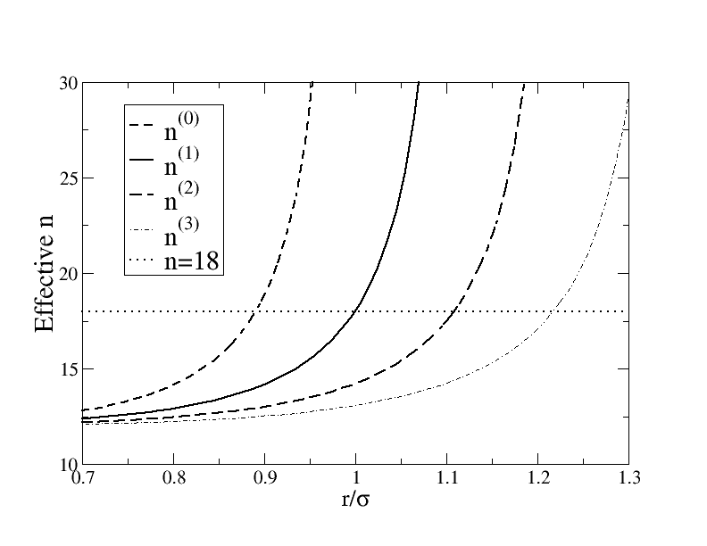
Figure 1: Effective power-law exponents defined by derivative ratios of different orders (Eqs. (10)), for the standard Lennard-Jones potential LJ(12,6). All converge to 12 at small $r$; they diverge when the derivative in the denominator vanishes, which happens for larger $r$, the higher the order of this derivative. The term “effective inverse power law” in this paper refers to a power law chosen to match $n^{(1)}$ at some point $r_{0}<r_{m}\sim 1.12\sigma$, the potential minimum where $n^{(1)}$ diverges. A convenient choice is to match at $r=\sigma$, giving 18. In subsections II.2 and II.3 we show that $n^{(2)}(r)$ plays an important role in the understanding of fluctuations associated with pair distances close to the potential minimum ($r_{m}\sim 1.12\sigma$).

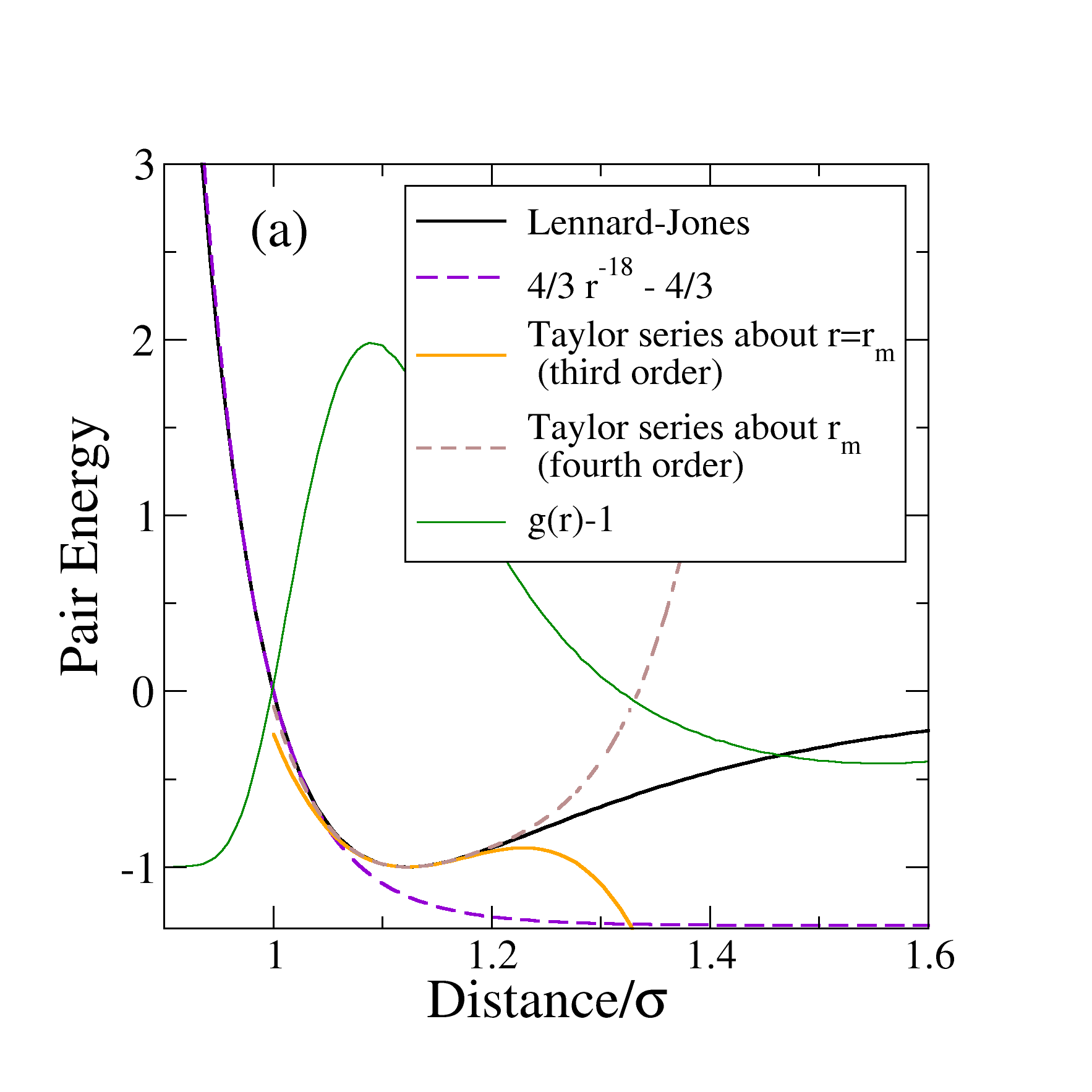
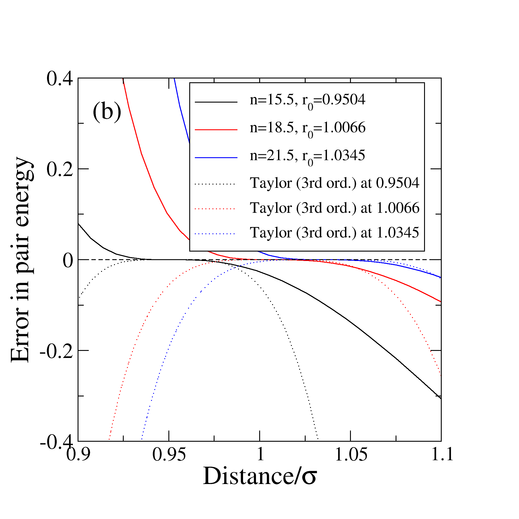
Figure 2: (Color online) (a) The Lennard-Jones potential $v_{LJ}(r)$ fitted by an effective power law potential $v_{PL}(r)=Ar^{-n}+B$ covering the most important part of the repulsive part of the potential. The exponent $n$ was chosen to be $18$ which optimizes agreement at $r_{0}=\sigma$, where the effective power law exactly matches not just $v_{LJ}$, but also its first two derivatives. Also shown are the Taylor series expansions of $v_{LJ}(r)$ about $r=r_{m}$ up to third and fourth order. The radial distribution function $g(r)-1$ (at $T=80$K, $p=0$) is also shown as a convenient reference for thinking about where contributions to potential energy and virial fluctuations come from. 0(b) Error made in approximating $v_{LJ}(r)$ with different effective power laws matched at different points $r_{0}$ and with Taylor expansions up to third order about the same point.

The fact that we can choose a function (an inverse power law in this case) to match a given function and its first two derivatives is nothing special by itself; after all, a Taylor series does the same. Examples of matching power laws and Taylor series up to fourth order, at different values of $r_{0}$, are shown in Fig. 2(b), where the errors $v_{LJ}(r)-v_{PL}(r)$ or $v_{LJ}(r)-v_{Taylor}(r)$ are plotted. The magnitude of the errors are similar in the range of $r$ shown, but note that in the Taylor series it was necessary to match third derivatives at $r_{0}$ to achieve this, so the inverse power-law description is more compact. Moreover the power-law representation is much more useful when it comes to representing the fluctuations of total energy and virial, because an inverse power law (and therefore the error) flattens out at a constant value at larger $r$, whereas the polynomial nature of the Taylor expansion means that away from the point of expansion, the error diverges rapidly (Fig. 2(a)).

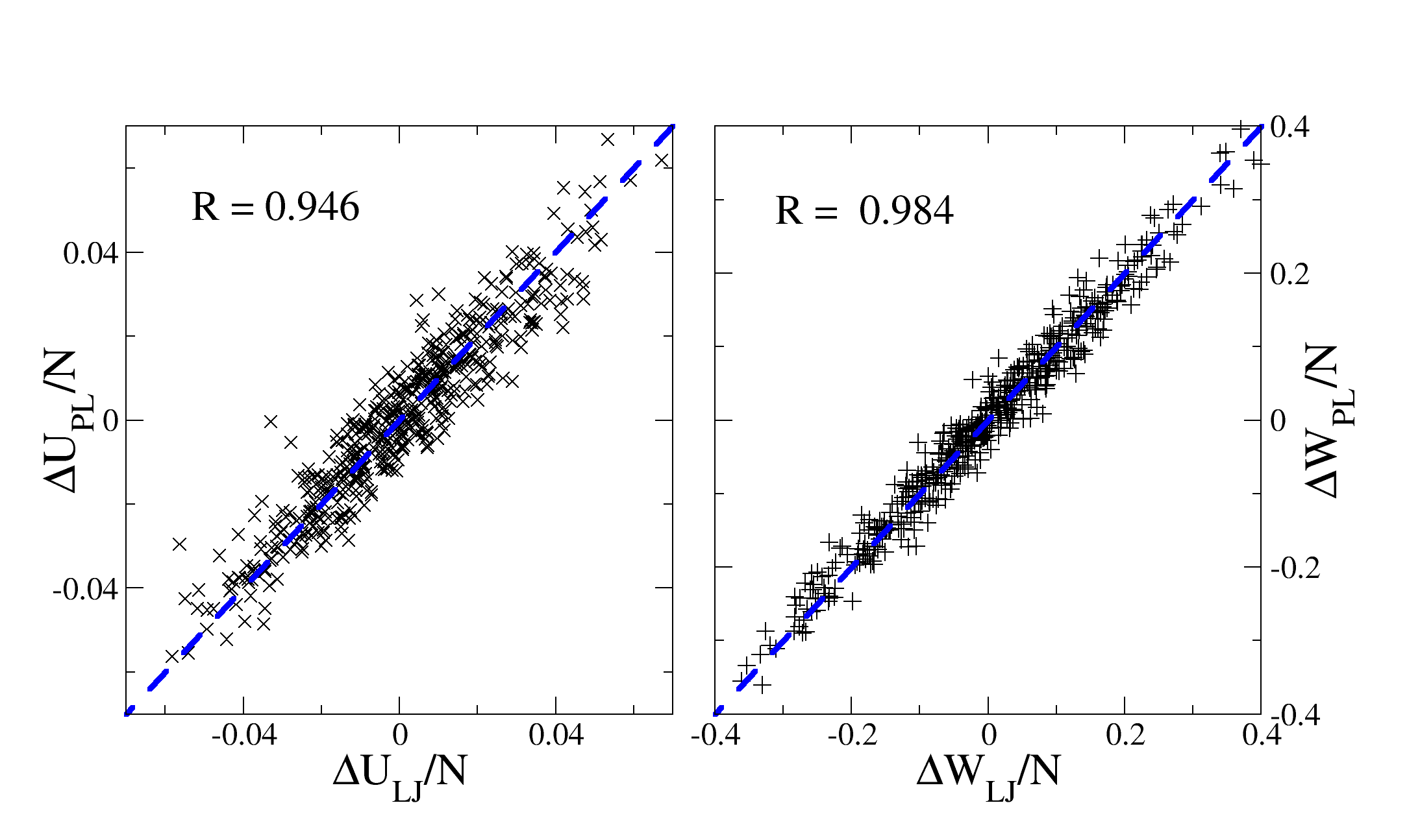
Figure 3: (Color online) Scatter-plot of true and “reconstructed” potential-energy and virial fluctuations (dimensionless units) for the LJ-liquid, where the reconstructed values $U_{PL}$ and $W_{PL}$ were calculated from the true configurations, assuming an inverse power-law potential with exponent 19.2; mean values have been subtracted off. The state point is the same as in Fig. 1 of paper I (zero average pressure, NVT ensemble). The correlation coefficients are displayed in the figures; the dashed lines indicate slope unity. The fact that actual and reconstructed fluctuations correlate strongly, and with slopes close to unity, support the idea that the $W,U$ correlation is derived from an effective inverse power-law potential dominating fluctuations.

We can test the validity of the power-law approximation for representing fluctuations in $W$ and $U$ as follows. For the purpose of computing the energy and virial of a configuration due to a pair interaction, all necessary information is contained in the instantaneous radial distribution function (RDF)Allen and Tildesley (1987)

$$g(r,t)\equiv\frac{2}{N\rho}\sum_{i<j}\delta(r-r_{ij}(t))/(4\pi r^{2}),$$ (12)

where $\rho=N/V$ with $N$ and $V$ being the number of particles and the system volume, respectively. From this $U$ and $W$ may be computed as

$$U_{LJ}(t)=\frac{N}{2}\rho\int_{0}^{\infty}\!dr\,4\pi r^{2}g(r,t)v_{LJ}(r)$$ (13)

$$W_{LJ}(t)=-\frac{N}{6}\rho\int_{0}^{\infty}\!dr\,4\pi r^{2}g(r,t)w_{LJ}(r).$$ (14)

Now, $U_{LJ}(t)$ is re-written as an inverse power-law potential plus a difference term, $U_{LJ}(t)=U_{PL}(t)+U_{\textrm{diff}}(t)$, where

$$U_{PL}(t) =\frac{N}{2}\rho\int_{0}^{\infty}dr\,4\pi r^{2}g(r,t)v_{PL}(r)$$ (15)

$$U_{\textrm{diff}}(t) =\frac{N}{2}\rho\int_{0}^{\infty}dr\,4\pi r^{2}g(r,t)(v_{LJ}(r)-v_{PL}(r))$$ (16)

and similarly $W_{LJ}(t)=W_{PL}(t)+W_{\textrm{diff}}(t)$. We do not include the additive constant with the power-law approximation; for practical reasons the potential function should be close to zero at a cut-off distance $r_{c}$ (adding a constant to $v_{PL}$ would only add an overall constant to $U_{PL}$). We refer to $U_{PL}(t)$ and $W_{PL}(t)$ as “reconstructed” potential energy and virial, respectively, to emphasize that the configurations are drawn from a simulation using the Lennard-Jones potential, but these quantities are calculated using the inverse power law. In Fig. 3, we show a scatter plot of the true and reconstructed values of $U$ and $W$, for the same state point ($p$ = 0, $T$ = 80K) as was shown in Figs. 1 and 2(a) of Paper I. Here the inverse power-law exponent was chosen to minimize the variances of the difference quantities, $\langle(\Delta U_{\textrm{diff}})^{2}\rangle$ and $\langle(\Delta W_{\textrm{diff}})^{2}\rangle$. These are minimized for $n=19.3$ and $19.1$, respectively, so we choose the value 19.2, which corresponds to matching the potentials at the distance 1.015$\sigma$. Note that what are actually plotted are the deviations from the respective mean values—the means $\langle U_{LJ}\rangle$ and $\langle U_{PL}\rangle$, for example, do not coincide. But the fluctuations are clearly highly correlated, and the data lie quite close to the blue dashed lines, marking slope unity. Specifically, the correlation coefficients are 0.946 for the potential energy and 0.984 for the virial. We can also check how much of the variance of $U_{LJ}$ is accounted for by $U_{PL}$, $\langle(\Delta U_{PL})^{2}\rangle/\langle(\Delta U_{LJ})^{2}\rangle$, and similarly for $W$. This is a sensible quantity because the ‘PL’ and ‘diff’ parts are almost uncorrelated for the choice $n=19.2$ (cross terms account for less than 1% of the total variance in each case). We find 92% for $U$ and 95% for $W$. Thus we see that the power law gives to a quite good approximation the fluctuations of $W$ and $U$. The correlation follows from this with $\gamma$ given by one third of the effective inverse power-law exponent, or 6.4 for this state point. The measured slope (Eq. (6)) was 6.3 corresponding to an effective exponent 18.9, about 2% smaller than the 19.3. A simpler way to determine the exponent would be three times the slope, although for some applications it could be advantageous to optimize the fit as described here.

II.2 Low temperature limit: anharmonic vibrations of a crystal

We turn our attention now to the fact that the correlation persists even for the crystallized samples (seen in Paper I in the lower left part of Fig. 4 and in Fig. 6). This is not trivial, because the physics of solids, both crystalline and amorphous systems, is generally dominated by fluctuations about mechanically stable structures, and therefore presumably (except perhaps at very high pressure) by the form of the potential near its minimum $r_{m}$, i.e., including distances larger than the minimum. Thus the idea of the effective inverse power law would seem to be inappropriate here—in particular since the effective exponent $n^{(1)}$ diverges at $r_{m}$—and there is apparently no reason why one should get a correlation as strong as in the liquid and with so similar a slope. In fact there is an interval of $r$ between $r_{m}$ and the minimum of the pair virial $-w(r)/3$ where $v(r)$ is increasing and $-w(r)/3$ is decreasing, which would lead if anything to a negative correlation between $W$ and $U$, when considering individual pair interactions. Moreover, one would expect that a harmonic approximation of the potential near the ground-state configuration would be an accurate representation of the dynamics in the low-temperature limit, but as we will see, the harmonic approximation actually implies negative $W,U$ correlation, which is not observed. In this subsection we show why the strong positive correlation persists, and why the slope $\gamma$ changes little going from liquid to crystal (at constant volume). Although the classical dynamics of a crystal is apparently of little importance, since in reality quantum effects dominate, it turns out to be very instructive to consider the low-temperature ($T\rightarrow 0$) classical limit, since what we find has significance also in the liquid phase (subsection II.3). The key ideas are (1) that the positive correlation emerges only after summing over all interactions—it is therefore a collective effect, rather than a single-pair effect, and (2) the constraint of fixed volume—it is important to recall from Paper I that the virial-potential-energy correlation only appears under fixed-volume conditions; different volumes give approximately the same slope but different offsets (Fig. 4 in Paper I).

II.2.1 The one-dimensional crystal

For maximum clarity we start by considering the simplest possible case, a one-dimensional (1D) crystal with periodic boundary conditions and only nearest-neighbor interactions. We also suppose that the lattice spacing $a_{c}$ is equal to the minimum of the potential; this assumption is not made in the subsequent treatment of the 3D crystal. In a crystal the particles stay close to their equilibrium positions. It therefore makes sense to expand the pair energy (we have in mind a general pair potential with a single minimum) as a Taylor series, leaving out constant terms but keeping third order terms:

$$U =\sum_{i}\left(\frac{1}{2}k_{2}(r_{i,i+1}-r_{m})^{2}+\frac{1}{6}k_{3}(r_{i,i+1}-r_{m})^{3}\right)$$

$$\equiv\frac{1}{2}k_{2}S_{2}+\frac{1}{6}k_{3}S_{3}$$ (17)

where $r_{i,i+1}$ is the distance between particles $i$ and $i+1$, $k_{p}$ is the $p$-th derivative of the pair potential at $r=r_{m}$, and we introduce the notation

$$S_{p}\equiv\sum_{i}(r_{i,i+1}-r_{m})^{p}.$$ (18)

The virial is

$$W= -\frac{1}{3}\sum_{i}\biggl{(}k_{2}r_{i,i+1}(r_{i,i+1}-r_{m})$$

$$\left.+\frac{k_{3}r_{i,i+1}}{2}(r_{i,i+1}-r_{m})^{2}\right)$$ (19)

which, by writing $r_{i,i+1}=r_{m}+(r_{i,i+1}-r_{m})$, can be rewritten as

$$W=-\frac{1}{3}\left(k_{2}\ r_{m}S_{1}+k_{2}S_{2}+\frac{k_{3}r_{m}}{2}S_{2}+\frac{k_{3}}{2}S_{3}\right).$$ (20)

Note that $U$ involves $S_{2}$ and $S_{3}$ while $W$ also has a first-order term with $S_{1}$. Evaluating the sum $S_{1}$ is very simple: $r_{i,i+1}$ can be expressed in terms of displacements from the equilibrium positions $u_{i}$ as $r_{i,i+1}=r_{m}+u_{i+1}-u_{i}$, giving for $S_{1}$

$$S_{1}=\sum_{i}(u_{i+1}-u_{i}).$$ (21)

Such a sum of consecutive relative displacements gives the change in separation of the two end particles. But the total sum must vanish, because by periodic boundary conditions the “end particles” are the same particle (it doesn’t matter which one), therefore $S_{1}=0$. In fact periodic boundary conditions are not necessary, only that the length is fixed. Since both $U$ and $W$ involve at lowest order $S_{2}$, which is positive semi-definite, at sufficiently low temperature we may drop the $S_{3}$ terms. Combining Eqs. (17) and (20) we find

$$W =-\frac{1}{3}\frac{k_{2}+k_{3}r_{m}/2}{k_{2}/2}U$$

$$=\frac{n^{(2)}(r_{m})}{3}U,$$ (22)

where we have written the coefficient in terms of the $p=2$ effective power-law exponent defined in Eq. (10). For LJ(a,b) the coefficient evaluates to $(a+b+1)/3$, which is $6.33$ for LJ(12,6), similar to the observed slope. This short calculation demonstrates the main point: summing over all interactions makes the first-order term in the virial vanish, and the second-order term is proportional to the second-order term in the potential energy. It is also worth noting that for a purely harmonic crystal we can take $k_{3}=0$, in which case Eq. (22) implies that there is perfect negative correlation, with a slope of -2/3.

II.2.2 The three-dimensional crystal

We now generalize this to three-dimensional crystals, which means allowing for transverse displacements. The calculation involves breaking overall sums into sums over one-dimensional chains within the crystal. We also relax the condition that the lattice constant coincides with the potential minimum, which is only realistic at low pressures. We still assume only nearest-neighbor interactions are relevant (this will be justified in the next subsection). Generalization to a disordered (amorphous) solidBinder and Kob (2005) should be possible, since we observe the correlation to hold also in that case. The calculation would necessitate, however, some kind of disorder averaging, which is beyond the scope of this paper.

We start by considering a simple cubic (SC) crystal of lattice constant $a_{c}$, with interactions only between nearest neighbors, so that the equilibrium bond length is $a_{c}$ for all bonds. The fact that such a crystal is mechanically unstable is irrelevant for the calculation. We shall see later that the result applies also to, for instance, an FCC crystal. We have the same kind of expansions about $r=a_{c}$ as above for $U$ and $W$, except a linear term is now included, since we no longer assume that $a_{c}=r_{m}$. An index $b$ is used to represent nearest-neighbor bonds and as for the 1D case we define

$$S_{p}\equiv\sum_{b}(r_{b}-a_{c})^{p}.$$ (23)

We then have for $U$ and $W$

$$U =\sum_{p=1}^{\infty}\frac{k_{p}}{p!}\sum_{\textrm{bonds}\,b}(r_{b}-a_{c})^{p}=\sum_{p=1}^{\infty}\frac{k_{p}}{p!}S_{p}$$ (24)

$$3W =\sum_{p=1}^{\infty}-\frac{k_{p}}{(p-1)!}\sum_{\textrm{bonds}\,b}r_{b}(r_{b}-a_{c})^{p-1}$$

$$=-\sum_{p=1}^{\infty}\frac{k_{p}a_{c}}{(p-1)!}S_{p-1}-\sum_{p=1}^{\infty}\frac{k_{p}}{(p-1)!}S_{p}$$

$$=-k_{1}a_{c}S_{0}-\sum_{p=1}^{\infty}\left(\frac{k_{p}}{(p-1)!}+\frac{k_{p+1}a_{c}}{p!}\right)S_{p}$$ (25)

where $k_{p}$ is the $p$-th derivative of the pair potential at $r=a_{c}$. It is convenient to define coefficients $C_{p}^{U}$ and $C_{p}^{W}$ of the dimensionless quantities $S_{p}/a_{c}^{p}$:

$$C_{p}^{U} \equiv\frac{k_{p}a_{c}^{p}}{p!}$$ (26)

$$C_{p}^{W} \equiv-\left(\frac{k_{p}a_{c}^{p}}{(p-1)!}+\frac{k_{p+1}a_{c}^{p+1}}{p!}\right)$$ (27)

Dropping the constant term $-k_{1}a_{c}S_{0}$ in $W$, since it plays no role for the fluctuations, we then have

$$U =\sum_{p=1}^{\infty}C_{p}^{U}\frac{S_{p}}{a_{c}^{p}}$$ (28)

$$3W =\sum_{p=1}^{\infty}C_{p}^{W}\frac{S_{p}}{a_{c}^{p}}$$ (29)

The ratio of corresponding coefficients is given by the $p$th order effective inverse power-law exponent:

$$C_{p}^{W}/C_{p}^{U}=-\left(p+\frac{k_{p+1}a_{c}}{k_{p}}\right)=n^{(p)}(a_{c}).$$ (30)

Thus for in the limit of small $a_{c}$, where these are all similar and close to the repulsive exponent in the potential (Fig. 1), the two expansions will be proportional to each other, to infinite order. Also worth noting for later use is that the $C_{p}$s in each series increase with $p$. For example

$$C_{2}^{U}/C_{1}^{U} =\frac{k_{2}a_{c}}{2k_{1}}=-\frac{1}{2}(n^{(1)}(a_{c})+1)$$ (31)

$$C_{2}^{W}/C_{1}^{W} =\frac{k_{2}a_{c}+k_{3}a_{c}^{2}/2}{k_{1}+k_{2}a_{c}}$$

$$=-\frac{1}{2}(n^{(1)}(a_{c})+1)\frac{n^{(2)}(a_{c})}{n^{(1)}(a_{c})}.$$ (32)

For $a_{c}$ between $\sigma$ and $r_{m}$, for LJ(12,6), the absolute values of these ratios lie in the intervals 9.5–$\infty$ and 6.7–9.5 respectively.

From dimensional considerations the variance of $S_{p}$ is proportional to $N\sigma_{u}^{2p}$, where $\sigma_{u}^{2}\propto T$ is the variance of single-particle displacements. At low $T$, therefore, we expect the $S_{1}$ terms to dominate, which causes a problem since $k_{1}$ changes sign at $r_{m}$, corresponding to the divergence of $n^{(1)}$. In 1D this was avoided by the exact vanishing of $S_{1}$. In 3D $S_{1}$ does not vanish exactly, but retains terms second order in displacements, and so contributes similarly to $S_{2}$. It turns out (see below) that $S_{1}$ and $S_{2}/a_{c}$ have similar variances and significant positive correlation, but in view of Eqs. (31) and (32) this is not even necessary for a strong $W,U$ correlation—the coefficients of the $S_{1}$ are relatively small so that it is still the $S_{2}$ terms that dominate. That is essentially the explanation of the strong correlations in the crystal, but we now continue the analysis in more detail in order to investigate how good it becomes in the limit $T\rightarrow 0$. These general considerations will be of use again in the following subsection, where we make a similar expansion of the fluctuations in the liquid state.

We need to evaluate $S_{1}$ and $S_{2}$ in terms of the relative displacements $\mathbf{u}_{b}$ of the pair of particles involved in bond $b$. We keep only terms up to second order in displacements, since we are interested in the limit of low-temperatures, so all $S_{3}$ terms in the expansion are dropped. In an SC crystal, all nearest neighbor bonds are parallel to one of the coordinate (crystal) axes. Consider all bonds along the $x$-axis. These may be grouped into rows of collinear bonds. The sum along a single row is almost analogous to the one-dimensional case, except that the bond length $r_{b}$ now also involves transverse displacements:

$$S_{p}^{\textrm{row}}=\sum_{b,\textrm{row}}(r_{b}-a_{c})^{p}$$ (33)

We write $r_{b}$ explicitly in terms of relative displacements and expand the resulting square root, dropping terms of higher order than the second in $u$:

$$r_{b}-a_{c} =((a_{c}+u_{b,x})^{2}+u_{b,y}^{2}+u_{b,z}^{2})^{1/2}-a_{c}$$

$$=a_{c}\left(1+\frac{2u_{b,x}}{a_{c}}+\frac{u_{b,x}^{2}}{a_{c}^{2}}+\frac{u_{b,y}^{2}+u_{b,z}^{2}}{a_{c}^{2}}\right)^{1/2}-a_{c}$$

$$=a_{c}\left(1+\frac{1}{2}\left(\frac{2u_{b,x}}{a_{c}}+\frac{u_{b,x}^{2}+u_{b,y}^{2}+u_{b,z}^{2}}{a_{c}^{2}}\right)\right.$$

$$\left.-\frac{1}{8}\left(\frac{2u_{b,x}}{a_{c}}\right)^{2}\right)-a_{c}$$

$$=u_{b,x}+\frac{u_{b,y}^{2}+u_{b,z}^{2}}{2a_{c}}.$$ (34)

Now, the sum over bonds in a given row of the parallel displacements $u_{b,x}$ vanishes for the same reasons as in the one-dimensional case. But when we sum the contributions to $S_{1}$ over the row, there are also second-order terms coming from the transverse displacements. Extending the sum to all bonds parallel to the $x$-axis, we have part of $S_{1}$, denoted $S_{1}^{x}$:

$$S_{1}^{x}=\sum_{b,x}\frac{u_{b,y}^{2}+u_{b,z}^{2}}{2a_{c}}=\sum_{b,x}\frac{|\mathbf{u}_{b,\perp}|^{2}}{2a_{c}}$$ (35)

where $\perp$ indicates the component of the relative displacement vector perpendicular to the bond direction. Writing it this way allows us to easily include the bonds parallel to the $y$- and $z$-axes, and the total $S_{1}$ is given by

$$S_{1}=\sum_{b}\frac{|\mathbf{u}_{b,\perp}|^{2}}{2a_{c}}.$$ (36)

Next we calculate $S_{2}$ to second order in relative displacements $\mathbf{u}_{b}$. Starting with $S_{2}^{x}$, the part containing only bonds in the $x$-direction, using Eq. (34) we get

$$S_{2}^{x}=\sum_{b,x}u_{b,x}^{2}=\sum_{b,x}|\mathbf{u}_{b,\parallel}|^{2}$$ (37)

where $\parallel$ means the part of the relative displacement that is parallel to the bond. Including all bonds,

$$S_{2}=\sum_{b}|\mathbf{u}_{b,\parallel}|^{2}.$$ (38)

Now we can return to our expressions for the potential-energy fluctuations (Eqs. (24) and (25)), keeping only terms in $S_{1}$ and $S_{2}$:

$$\Delta U=k_{1}S_{1}+\frac{k_{2}}{2}S_{2}=\frac{k_{1}}{2a_{c}}\sum_{b}|\mathbf{u}_{b,\perp}|^{2}+\frac{k_{2}}{2}\sum_{b}|\mathbf{u}_{b,\parallel}|^{2}.$$ (39)

Similarly, for the virial

$$3W =-k_{2}a_{c}S_{1}-\frac{k_{3}a_{c}}{2}S_{2}-k_{1}S_{1}-k_{2}S_{2}$$

$$=-\left(\frac{k_{1}}{2a_{c}}+\frac{k_{2}}{2}\right)\sum_{b}|\mathbf{u}_{b,\perp}|^{2}-\left(k_{2}+\frac{k_{3}a_{c}}{2}\right)\sum_{b}|\mathbf{u}_{b,\parallel}|^{2}.$$ (40)

II.2.3 Statistics of $S_{1}$ and $S_{2}$

It is clear that the $\parallel$ and $\perp$ sums are not equal, although they must be correlated to some extent: If written in terms of single-particle displacements rather than relative displacements for bonds, a term such as $|\mathbf{u}_{b,\parallel}|^{2}$ for a bond in the $x$-direction becomes

$$(u_{\mathbf{R}+a_{c}\hat{\i},x}-u_{\mathbf{R},x})^{2}=u_{\mathbf{R}+a_{c}\hat{\i},x}^{2}+u_{\mathbf{R},x}^{2}-2u_{\mathbf{R}+a_{c}\hat{\i},x}u_{\mathbf{R},x},$$ (41)

where $\mathbf{R}$ is a lattice vector used to index particles. Summing over bonds gives

$$S_{2}=2\sum_{\mathbf{R}}|\mathbf{u}_{\mathbf{R}}|^{2}-2\sum\textrm{(para. cross terms)}$$ (42)

where the cross terms are products of the parallel components of displacements on neighboring particles. For $S_{1}$ we have something similar:

$$S_{1}a_{c}=2\sum_{\mathbf{R}}|\mathbf{u}_{\mathbf{R}}|^{2}-2\sum\textrm{(perp. cross terms)}$$ (43)

where here the cross terms involve transverse components. Since the term $\sum_{\mathbf{R}}|\mathbf{u}_{\mathbf{R}}|^{2}$ appears in both $S_{1}$ and $S_{2}$, these are correlated to some extent, but not 100% since different cross terms appear (note that if it were 100%, then $W$ and $U$ would both be proportional to $S_{2}\propto S_{1}$ and also correlated 100%). Before considering to what extent they are correlated, let us see how much of a difference it makes. Suppose the quantities $S_{1}a_{c}$ and $S_{2}$ have variances $\sigma_{1}^{2}$ and $\sigma_{2}^{2}$, respectively, and are correlated with correlation coefficient $R_{S}$. Using the coefficients introduced in Eqs. (26) and (27)

$$Ua_{c}^{2} =C_{1}^{U}(S_{1}a_{c})+C_{2}^{U}S_{2}$$

$$3Wa_{c}^{2} =C_{1}^{W}(S_{1}a_{c})+C_{2}^{W}S_{2}.$$ (44)

From this we obtain an expression for the $W,U$ correlation coefficient by forming the appropriate products and taking averages:

$$R=\frac{C_{1}^{U}C_{1}^{W}\sigma_{1}^{2}+C_{2}^{U}C_{2}^{W}\sigma_{2}^{2}+(C_{1}^{U}C_{2}^{W}+C_{1}^{W}C_{2}^{U})\sigma_{1}\sigma_{2}R_{S}}{\sqrt{(C_{1}^{U})^{2}\sigma_{1}^{2}+(C_{2}^{U})^{2}\sigma_{2}^{2}+2C_{1}^{U}C_{2}^{U}\sigma_{1}\sigma_{2}R_{S}}\sqrt{(C_{1}^{W})^{2}\sigma_{1}^{2}+(C_{2}^{W})^{2}\sigma_{2}^{2}+2C_{1}^{W}C_{2}^{W}\sigma_{1}\sigma_{2}R_{S}}}$$ (45)

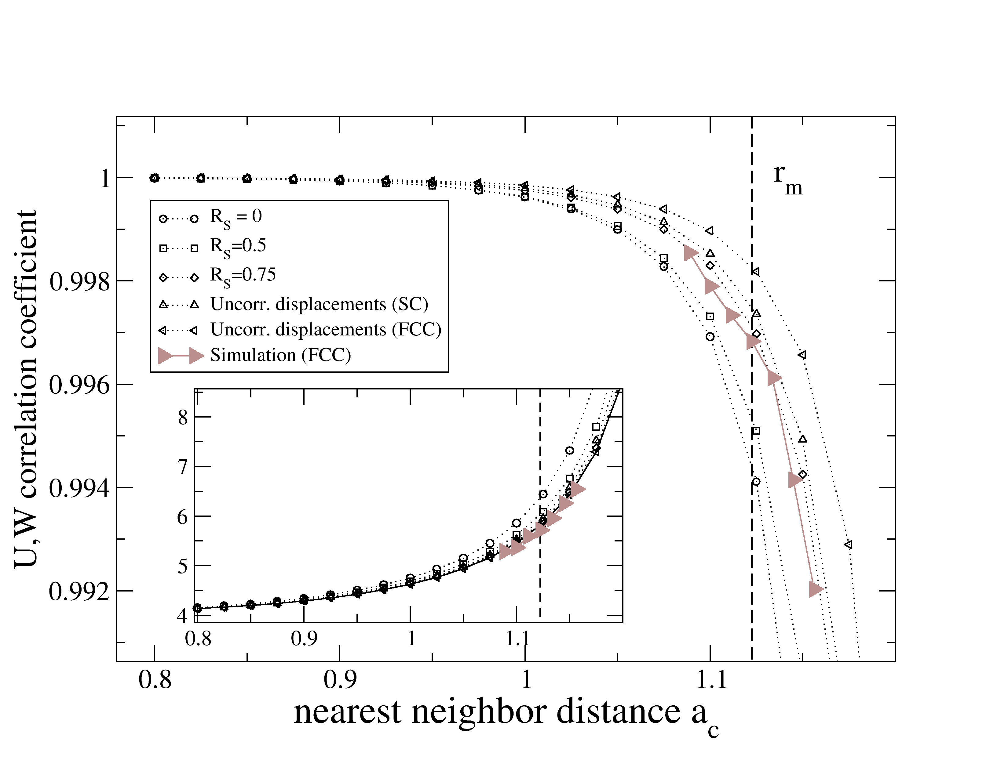
Figure 4: (Color online) Plots of predicted $W,U$ correlation coefficient for $T\rightarrow 0$ for a crystal of LJ(12,6) particles for different degrees of correlation between the quantities $S_{1}a_{c}$ and $S_{2}$, and of low-temperature simulation data. The first three curves (counting from the bottom) assume the variances of $S_{1}a_{c}$ and $S_{2}$ are equal, and their correlation coefficient $R_{S}$ is 0, 0.5 and 0.75, respectively. The fourth curve (up-triangles) results from considering a simple cubic lattice and assuming individual particles have uncorrelated Gaussian-distributed displacements, leading to specific values for the variances and covariance of $S_{1}a_{c}$ and $S_{2}$. The fifth (left-triangles) shows the same estimate for an FCC lattice. The right-triangles are data from an NVT simulation of a perfect FCC crystal at $T=0.0002$K. The conclusion from this figure is that $R$ does not tend to unity as $T\rightarrow 0$, although it becomes extremely close. The inset shows the corresponding slopes $\gamma$ (Eq. (6)).

Table 1: Statistics of $S_{1}a_{c}$ and $S_{2}$ assuming uncorrelated particle displacements with variance $\sigma_{u}^{2}$ for each Cartesian component, for simple cubic (SC) and face-centered cubic (FCC) lattices.

	SC	FCC
$\langle S_{1}a_{c}\rangle$	$6N\sigma_{u}^{2}$	$12N\sigma_{u}^{2}$
$\langle S_{2}\rangle$	$6N\sigma_{u}^{2}$	$12N\sigma_{u}^{2}$
$\textrm{var}(S_{1}a_{c})$	$30N\sigma_{u}^{4}$	$108N$
$\textrm{var}(S_{2}$)	$36N\sigma_{u}^{4}$	$120N$
$\textrm{cov}(S_{1}a_{c},S_{2})$	$24N\sigma_{u}^{4}$	$96N$
$R_{S}$	0.73	0.84

This estimation of $R$ is plotted in Fig. 4 as a function of lattice constant for $R_{S}=$0, 0.5 and 0.75, for the case $\sigma_{1}=\sigma_{2}$. Clearly the value of $R_{S}$ makes little difference in the region of interest, $a_{c}\sim r_{m}$ or less, where $R$ is above 0.99. Note that all curves drop dramatically as the lattice constant approaches the inflection point ($k_{2}=0$) of the potential (the precise value at which $R$ becomes zero depends on the statistics of $S_{1}a_{c}$ and $S_{2}$). In this regime, however, higher-order terms in displacements, including $S_{3}$, $S_{4}$, etc., become more important, and because of Eq. (30) their inclusion tends to restore $R$ to a high value (we have not calculated their effect in detail). Also plotted is the estimation of $R$ obtained by assuming that particle displacements are uncorrelated and Gaussian distributed with variance $\sigma_{u}^{2}$ for each (Cartesian) component, corresponding to an Einstein model of the vibrational dynamics. In this case tedious, but straightforward algebra allows the means and (co-)variances of $S_{1}a_{c}$ and $S_{2}$ to be calculated explicitly for a given lattice. The results for SC and FCC are given in Table 1. Notice that the variance of $S_{2}$ is somewhat larger than that of $S_{1}a_{c}$, while their means are equal. This can be traced to the fact the latter contains twice as many cross terms as the former, and a factor of one half, so the contribution from such terms to the mean is the same in both cases, while the contribution to the variance is smaller for $S_{1}a_{c}$. From the (co)-variances we find the correlation coefficient $R_{S}=0.73$ and $R_{S}=0.84$ for the SC and FCC cases respectively. These are also plotted in Fig. 4. A more exact calculation would take into account the true normal modes of the crystal, but would yield little of use: Data from the crystal simulations at very low temperature, also plotted in Fig. 4 agree within estimated numerical errors with both the SC and FCC estimates. The key point of this figure—that $R$ is close to but less than 1—apparently would change little by taking the true crystal dynamics into account. In particular it is important to note that if $R=1$ exactly, then this would be true no matter what kind of weighted average of configurations is taken (what kind of ensemble), so a value less than unity in the Einstein approximation is sufficient to disprove the hypothesis that $R\rightarrow 1$ as $T\rightarrow 0$.

II.2.4 The role of the coefficients $C_{1,2}^{U,W}$

Since the detailed statistics of $S_{1}$ and $S_{2}$ have little effect on the $W,U$ correlation, it must be mainly due to the numerical values of the coefficients $C_{1,2}^{U,W}$. We can estimate the effect of these by assuming $S_{1}a_{c}$ and $S_{2}$ have equal variance and are uncorrelated ($R_{S}=0$). Then according to Eq. (45) the $W,U$ correlation coefficient is

$$R=\frac{C_{1}^{U}C_{1}^{W}+C_{2}^{U}C_{2}^{W}}{\sqrt{(C_{1}^{U})^{2}+(C_{2}^{U})^{2}}\sqrt{(C_{1}^{W})^{2}+(C_{2}^{W})^{2}}}$$ (46)

which has the form of the cosine of the angle between two vectors $\mathbf{C}^{U}\equiv(C_{1}^{U},C_{2}^{U})$ and $\mathbf{C}^{W}\equiv(C_{1}^{W},C_{2}^{W})$. Thus the closeness of $R$ to unity indicates that these vectors are nearly parallel. The tangents of the angles these vectors make with the $C_{1}$ axis in $(C_{1},C_{2})$-space are given by Eqs. (31) and (32); clearly the two angles become equal in the limit of small $a_{c}$, where $n^{(1)}$ and $n^{(2)}$ converge. On the other hand, for $a_{c}\sim r_{m}$ where $k_{1}=0$ and $n^{(1)}$ diverges, the two vectors are

$$\mathbf{C}^{U} =(0,k_{2}/2)a_{c}^{2}$$

$$\mathbf{C}^{W} =-(k_{2},k_{2}+k_{3}a_{c}/2)a_{c}^{2}=-k_{2}a_{c}^{2}(1,1-\frac{1}{2}(n^{(2)}+2))$$

$$=k_{2}a_{c}^{2}(-1,\frac{n^{(2)}}{2}).$$ (47)

Clearly $\mathbf{C}^{U}$ is parallel to the $C_{2}$ axis while $\mathbf{C}^{W}$ deviates from it by an angle of order $2/n^{(2)}\sim 1/10$. The $W,U$ correlation coefficient is then $R=\cos(1/10)\sim 1-\frac{1}{2}(1/10)^{2}\sim 0.995$, in agreement with the bottom curve (circles) in the main part of Fig. 4. In this case ($a_{c}=r_{m}$, $k_{1}=0$, $S_{1}a_{c}$ and $S_{2}$ uncorrelated with equal variance), we can obtain a simple expression for the slope

$$\gamma =\sqrt{\frac{(C_{1}^{W})^{2}+(C_{2}^{W})^{2}}{(C_{1}^{U})^{2}+(C_{2}^{U})^{2}}}=\frac{k_{2}}{3}\sqrt{\frac{1+(n^{(2)}/2)^{2}}{(k_{2}/2)^{2}}}$$

$$=\frac{2}{3}\sqrt{1+(n^{(2)}/2)^{2}}\sim\frac{n^{(2)}}{3}$$ (48)

consistent with the result from the one-dimensional case.

Thus when we look at the “collective” correlations in the crystal we naturally get a slope involving the effective power-law exponent $n^{(2)}$. Since the latter evaluated at the potential minimum is similar to $n^{(1)}$ at the zero of the potential, the slope is similar to that seen in the liquid phase. On the other hand, it is more typical to think about crystal dynamics starting from a harmonic approximation, adding in anharmonic terms when necessary for higher accuracy. How does that work here? If we set $k_{3}=0$ as well as $k_{1}=0$, so we consider the purely harmonic system with the nearest neighbor distance at the minimum of the potential, then we have $\mathbf{C}^{U}=(0,k_{2}/2)$ and $\mathbf{C}^{W}=-(k_{2}/3)(1,1)$. These are not close to being parallel, so the correlation will be weaker (coming mainly from that of $S_{1}$ and $S_{2}$), but more particularly, it will be negative, thus qualitatively different from the anharmonic case. Thus the presence of the $k_{3}$ affects the results at arbitrarily low temperature, so the harmonic approximation is never good enough. This is reminiscent of thermal expansion, which does not occur for a purely harmonic crystal. In fact, the Grüneisen parameter for a 1D crystal with nearest neighbor interactions may be shownAshcroft and Mermin (1976) to be equal to $1+n^{(2)}(a_{c})/2$.

Finally we consider the more realistic FCC crystal. First note that Eqs. (36) and (38) are unchanged as long as $a_{c}$ is now interpreted as the nearest-neighbor distance rather than the cubic lattice spacing: Each position in an FCC lattice has 12 nearest neighbors, four located in each of three mutually orthogonal planes. Taking the $xy$ and parallel planes first, the neighbors are located along the diagonal directions with respect to the cubic crystal axes. As before we can do the sum first over bonds forming a row, then over all parallel rows. For a given plane there are two orthogonal sets of rows, but the form of the sums in Eqs. (36) and (38) includes all bonds. The results of the calculation of (co)-variances of $S_{1}$ and $S_{2}$ in the Einstein model of the dynamics are changed in a way that in fact increases their mutual correlation and therefore the $W,U$ correlation, as shown in Table 1 and Fig. 4.

To summarize this subsection, the correlation in the crystal is an anharmonic effect that persists in the limit $T\rightarrow 0$. It works because (1) the constraint of fixed volume causes the terms in $U$ and $W$ that are first order in particle displacements to cancel and (2) the coefficients of the “transverse” second-order terms are small compared to those of the “parallel” ones, a fact which can be traced to the resemblance of the potential to a power law at distances shorter than the potential minimum. “Small” here means of order 1/10, which leads to over 99% correlation because $R$ is essentially the cosine of this quantity. In one dimension there are no transverse displacements and the correlation is 100% as $T\rightarrow 0$; in more than one dimension as $T\rightarrow 0$ the correlation is very close to unity, but never 100%.

To gain a more complete insight into the fluctuations, we next present an analysis which clarifies exactly the contributions to fluctuations from different distances, without approximations, now again with the liquid case in mind.

II.3 Fluctuation modes

In the last two subsections we considered single-pair effects (associated with $r<r_{m}$) and collective effects (associated with $r\sim r_{m}$), respectively. In this section we focus on contributions from particular pair separations without keeping track of which actual particles are involved. We identify the contributions to $U$ and $W$ coming from all pairs whose separation lies within a fixed small interval of separations $r$; fluctuations in the number of such pairs generate fluctuations in the the contributions. By considering all intervals we can systematically analyze the variances and covariances of $U$ and $W$ in terms of pair separation, which is the purpose of this section.

The instantaneous values of $U$ and $W$ are given by Eq. (13) and (14), generalized to an arbitrary pair potential. By taking a time (or ensemble) average we get corresponding expressions for $\langle U\rangle$ and $\langle W\rangle$ in terms of $g(r)\equiv\langle g(r,t)\rangle$, the usual thermally averaged RDF. Now we consider the variances $\langle(\Delta U)^{2}\rangle$ and $\langle(\Delta W)^{2}\rangle$, and the covariance $\langle\Delta U\Delta W\rangle$. Starting with, for example, $\Delta U(t)=4\pi\rho N/2\int_{0}^{\infty}drr^{2}\,v(r)\Delta g(r,t)$, where $\Delta g(r,t)\equiv g(r,t)-g(r)$, averaging and taking everything except $\Delta g(r,t)$ outside the average, we have

$$\langle(\Delta U)^{2}\rangle = (4\pi\rho N/2)^{2}\int_{0}^{\infty}\!dr_{1}\,r_{1}^{2}\int_{0}^{\infty}\!dr_{2}\,r_{2}^{2}v(r_{1})v(r_{2})\langle\Delta g(r_{1},t)\Delta g(r_{2},t)\rangle$$ (49)

$$\langle(\Delta W)^{2}\rangle = (4\pi\rho N/2)^{2}\int_{0}^{\infty}\!dr_{1}\,r_{1}^{2}\int_{0}^{\infty}\!dr_{2}\,r_{2}^{2}w(r_{1})w(r_{2})\langle\Delta g(r_{1},t)\Delta g(r_{2},t)\rangle$$ (50)

$$\langle\Delta U\Delta W\rangle = (4\pi\rho N/2)^{2}\int_{0}^{\infty}\!dr_{1}\,r_{1}^{2}\int_{0}^{\infty}\!dr_{2}\,r_{2}^{2}v(r_{1})w(r_{2})\langle\Delta g(r_{1},t)\Delta g(r_{2},t)\rangle.$$ (51)

Clearly the quantity which contains the essential statistical information about the fluctuations is $\langle\Delta g(r_{1},t)\Delta g(r_{2},t)\rangle$, the covariance of the RDF with itself. Its magnitude is inversely proportional to $N$, so that $\langle(\Delta U)^{2}\rangle$ is proportional to $N$, as it should be. The variances of $U$ and $W$ and their covariance are integrals of this function with different weightings. To make further progress, we integrate the integrands for the variances over $M\times M$ “blocks” in $r_{1},r_{2}$-space. This is equivalent to considering the energy, say, as the following sum of $M$ interval-energies:

$$U(t)=\sum_{a=1}^{M}U_{a}(t)$$ (52)

where the interval-energy $U_{a}(t)$ is defined as the integral between boundaries $r_{a}$ and $r_{a+1}$:

$$U_{a}(t)\equiv\frac{N}{2}\rho\int_{r_{a}}^{r_{a+1}}dr\,4\pi r^{2}g(r,t)v(r).$$ (53)

The virial can be similarly represented as a sum of contributions from the same $r$-intervals, $W(t)=\sum_{a=1}^{M}W_{a}(t)$. From now on we consider the primary fluctuating quantities to be $U_{a}(t)$ and $W_{a}(t)$ and seek to understand the correlation between their respective sums in terms of correlations between particular $U_{a}$s and $W_{a}$s. In order to achieve a reasonable degree of spatial resolution, we do not make the intervals (blocks) too big, and choose an interval width of 0.05. This gives $M$= 42 intervals: $U_{1}$ is the contribution to the energy coming from pairs with separation in the range 0.85 to 0.9, marking the lower limit of non-zero RDF, while $U_{42}$ refers to the range 2.9 to 2.95, marking the cutoff distance of the potential used here. We shall see explicitly that only distances up to around 1.4 contribute significantly to the fluctuations. We denote deviations from the mean as, e.g., $\Delta U_{a}=U_{a}-\langle U_{a}\rangle$ with the angle brackets representing the time (or ensemble) average.

Table 2: First ten eigenvalues of the super-covariance matrix (Eq. (66)), their fractional contributions to the three (co-)variances (Eqs. (63)–(65)) and their effective slopes (Eq. (68)), for the SCLJ liquid with parameters as in Fig. 1 of Paper I ($\rho$=34.6 mol/l, $T$=80K). Contributions from the dominant four eigenvectors are in boldface. The last three rows list sums of the third, fourth and fifth columns over, respectively, the dominant four, the first ten, and all $2M$ eigenvectors. The sum of the fifth column over all eigenvectors should be compared (see Eq. (65)) to the $R=$0.939 listed in Table I of Paper I.

index	eigenval.	$U$-var. contr.	$W$-var. contr.	corr. coeff. contr.	effective slope
1	1.73	0.01	0.01	0.01	5.38
2	1.55	0.04	0.06	0.05	7.63
3	1.11	0.24	0.15	0.19	4.98
4	0.87	0.25	0.25	0.25	6.34
5	0.78	0.20	0.14	0.17	5.27
6	0.58	0.11	0.17	0.13	7.80
7	0.34	0.02	0.05	0.03	10.14
8	0.23	0.01	0.03	0.01	13.67
9	0.13	0.00	0.01	0.00	116.19
10	0.10	0.01	0.00	-0.00	-3.63
$\sum_{3,\ldots,6}$	-	0.797	0.709	0.742	-
$\sum_{1,\ldots,10}$	-	0.884	0.877	0.849	-
$\sum_{1,\ldots,2M}$	-	1.000	1.000	0.938	-

We are interested in the covariance of the $U_{a}$s with themselves (including $\langle\Delta U_{a}\Delta U_{b}\rangle$, $a\neq b$), the $W_{a}$s with themselves, and the $U_{a}$s with the $W_{a}$s. These covariances are just what is obtained by integrating the integrands in Eqs. (49), (50), and (51) over the block defined by the corresponding intervals for $r_{1}$ and $r_{2}$. These values are conveniently represented using matrices $\mathbf{\Delta}^{UU}$, $\mathbf{\Delta}^{WW}$, and $\mathbf{\Delta}^{UW}$ defined as

$$(\mathbf{\Delta}^{UU})_{ab}=\langle\Delta U_{a}\Delta U_{b}\rangle,$$ (54)

$$(\mathbf{\Delta}^{WW})_{ab}=\langle\Delta W_{a}\Delta W_{b}\rangle,$$ (55)

and

$$(\mathbf{\Delta}^{UW})_{ab}=\langle\Delta U_{a}\Delta W_{b}\rangle.$$ (56)

Note that the sum of all elements of $\mathbf{\Delta}^{UU}$ is the energy variance, since it reproduces the double-integral of Eq. (49); similarly for the other two matrices:

$$\langle(\Delta U)^{2}\rangle =\sum_{a,b}(\mathbf{\Delta}^{UU})_{ab}$$ (57)

$$\langle(\Delta W)^{2}\rangle =\sum_{a,b}(\mathbf{\Delta}^{WW})_{ab}$$ (58)

$$\langle\Delta U\Delta W\rangle =\sum_{a,b}(\mathbf{\Delta}^{UW})_{ab}.$$ (59)

At this point we make one further transformation. Define new matrices $\mathbf{\Delta}^{UU*}$, $\mathbf{\Delta}^{WW*}$, $\mathbf{\Delta}^{UW*}$ by

$$\mathbf{\Delta}^{UU*}\equiv\mathbf{\Delta}^{UU}/\langle(\Delta U)^{2}\rangle,$$ (60)

$$\mathbf{\Delta}^{WW*}\equiv\mathbf{\Delta}^{WW}/\langle(\Delta W)^{2}\rangle,$$ (61)

and

$$\mathbf{\Delta}^{UW*}\equiv\mathbf{\Delta}^{UW}/\sqrt{\langle(\Delta U)^{2}\rangle\langle(\Delta W)^{2}\rangle}.$$ (62)

This is equivalent to normalizing the $U_{a}$s by the standard deviation $\sqrt{\langle(\Delta U)^{2}\rangle}$ and the $W_{a}$s by $\sqrt{\langle(\Delta W)^{2}\rangle}$ respectively. The elements of $\mathbf{\Delta}^{UU*}$, $\mathbf{\Delta}^{WW*}$ and $\mathbf{\Delta}^{UW*}$ can be thought of as representing, in some sense, what fraction of the total (co-)variance is contributed by the corresponding block. Normalized in this way, the sum over all elements of $\mathbf{\Delta}^{UU*}$ and $\mathbf{\Delta}^{WW*}$ is exactly unity and that for $\mathbf{\Delta}^{UW*}$ equals the correlation coefficient $R$:

$$\sum_{a,b}(\mathbf{\Delta}^{UU*})_{ab} =1$$ (63)

$$\sum_{a,b}(\mathbf{\Delta}^{WW*})_{ab} =1$$ (64)

$$\sum_{a,b}(\mathbf{\Delta}^{UW*})_{ab} =R.$$ (65)

To make a direct analysis of all possible co-variances, we now construct a larger $2M\times 2M$ matrix by placing $\mathbf{\Delta}^{UU*}$ and $\mathbf{\Delta}^{WW*}$ on the diagonal blocks, and $\mathbf{\Delta}^{UW*}$ and its transpose on the off-diagonal blocks:

$$\mathbf{\Delta}^{Sup}\equiv\left[\begin{array}[]{cc}\mathbf{\Delta}^{UU*}&\mathbf{\Delta}^{UW*}\\ (\mathbf{\Delta}^{UW*})^{T}&\mathbf{\Delta}^{WW*}\end{array}\right].$$ (66)

This “super-covariance” matrix contains all the information about the covariance of the contributions of energy and virial with each other. This symmetric and positive semidefinite matrix can be separated into additive contributions by spectral decomposition as

$$\mathbf{\Delta}^{Sup}=\sum_{\alpha}\lambda_{\alpha}v_{\alpha}v_{\alpha}^{T}$$ (67)

where $v_{\alpha}$ is the normalized eigenvector whose (non-negative) eigenvalue is $\lambda_{\alpha}$—this follows from the diagonalization of the matrix. Thus we decompose the super-covariance into a sum of parts. This method of accounting for the variance of many variables is the basis of the technique known as Principal Component Analysis (PCA), which is a workhorse of multivariate data analysis.Esbensen et al. (2002) The eigenvectors represent statistically independent “modes of fluctuation”; the corresponding eigenvalue is the part of the variance within the 2$M$-dimensional space accounted for by the mode. PCA is most effective when the eigenvectors associated with the largest few eigenvectors account for most of the variance in the set of fluctuating quantities. For example in the extreme case where one eigenvector accounts for over 99% of the variance, we could claim that all the different apparently random fluctuations of the different contributions to energy and virial were moving in a highly coordinated way, such that a single parameter (say, the value of any one of them) would be enough to give the values of all.

In our case we are not necessarily interested in the modes with the largest eigenvalues: a large eigenvalue could describe a fluctuation mode where the individual $U_{a}$s and $W_{a}$s change a lot, but their respective sums do not; this would correspond to the contributions from one interval increasing while those in others decrease, in such a way that the total is roughly constant. What we really want are those modes which contribute a lot to the variance of energy and virial, and to their covariance. This is easy to do by summing all elements in the appropriate block of the matrix $\lambda_{\alpha}v_{\alpha}v_{\alpha}^{T}$ where $v_{\alpha}$, $\lambda_{\alpha}$ are the normalized eigenvector and eigenvalue in question. In Table 2 we list the first ten eigenvalues in decreasing order, along with their contributions to the normalized variances of energy, virial, and their covariance—the normalized covariance being equal to $R_{W.U}$. In addition, an “effective slope” for each mode is obtained from the $\alpha^{\textrm{th}}$ eigenvector as

$$\gamma_{\alpha}=\sqrt{\frac{\langle(\Delta W)^{2}\rangle}{\langle(\Delta U)^{2}\rangle}}\frac{\sum_{a=M+1}^{2M}(v_{\alpha})_{a}}{\sum_{b=1}^{M}(v_{\alpha})_{b}}=\gamma\frac{\sum_{a=M+1}^{2M}(v_{\alpha})_{a}}{\sum_{b=1}^{M}(v_{\alpha})_{b}}$$ (68)

where the numerator gives the sum of virial contributions for that mode, and the denominator the sum of energy contributions. The factor in front, which is numerically equal to the overall slope $\gamma$, accounts for the standard deviation that we normalized the $U_{a}$s and $W_{a}$s by to define the matrices $\mathbf{\Delta}^{UU*}$, $\mathbf{\Delta}^{WW*}$ and $\mathbf{\Delta}^{UW*}$.

In the above equation, it looks like $\gamma_{\alpha}$ is determined by the overall $\gamma$, whereas we could expect more the opposite, that the overall slope is somehow an average of the individual effective mode slopes. It looks like this because of the normalization choice we made in determining the decomposition. We can relate the $\gamma_{\alpha}$ to the $\gamma$ in a more meaningful way by writing the sums in Eqs.  (63) and (64) in terms of the spectral decomposition Eq. (67):

$$1 =\frac{\sum_{a,c}\mathbf{\Delta}^{WW}_{a,c}}{\sum_{b,d}\mathbf{\Delta}^{UU}_{b,d}}=\frac{\sum_{\alpha}\sum_{a,c>M}\lambda_{\alpha}(v_{\alpha})_{a}(v_{\alpha})_{c}}{\sum_{\beta}\sum_{b,d\leq M}\lambda_{\beta}(v_{\beta})_{b}(v_{\beta})_{d}}$$ (69)

$$=\frac{\sum_{\alpha}\lambda_{\alpha}(\sum_{a>M}(v_{\alpha})_{a})^{2}}{\sum_{\beta}\lambda_{\beta}(\sum_{b\leq M}(v_{\beta})_{b})^{2}}$$ (70)

$$=\frac{\sum_{\alpha}\lambda_{\alpha}(\gamma_{\alpha}/\gamma)^{2}(\sum_{a\leq M}(v_{\alpha})_{a})^{2}}{\sum_{\beta}\lambda_{\beta}(\sum_{b\leq M}(v_{\beta})_{b})^{2}}$$ (71)

where in the last step Eq. (68) was used. Multiplying both sides by $\gamma^{2}$ we get an expression for the latter as a weighted average of the squares of the $\gamma_{\alpha}$:

$$\gamma^{2}=\frac{\sum_{\alpha}X_{\alpha}\gamma_{\alpha}^{2}}{\sum_{\beta}X_{\beta}}$$ (72)

where the weight of a given mode slope $\gamma_{\alpha}$ is (apart from normalization) $X_{\alpha}\equiv\lambda_{\alpha}(\sum_{a\leq M}(v_{\alpha})_{a})^{2}$, combining the eigenvalue and the square of the summed “energy part” of the corresponding eigenvector.

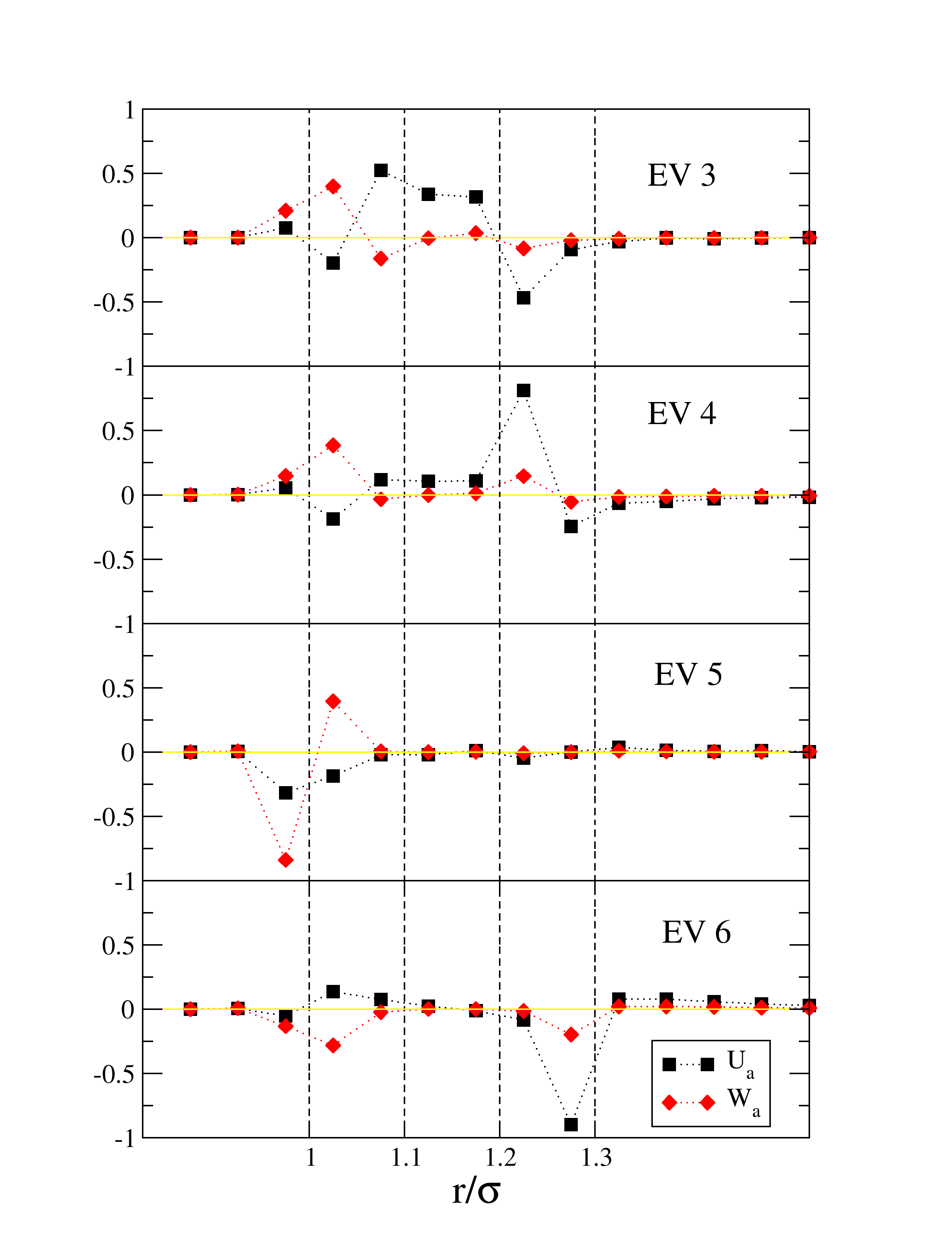
Figure 5: (Color online)Representations of the eigenvectors 3,4,5, and 6 of the super-covariance matrix. Squares represent variation in $U_{a}$ values for a mode; diamonds represent variation in $W_{a}$ values.

Now we can notice that the third, fourth, fifth and sixth eigenvectors, to be referred to respectively as EV3, EV4, EV5, and EV6, account for most of the three (co-)variances (totalling 0.80 out of 1.00, 0.71 out of 1.00 and 0.74 out of 0.94 for variance of $U$, variance $W$, and correlation coefficient, respectively). These four eigenvectors are represented in Fig. 5. We observe that, as expected, most of the fluctuations are associated with pair-separations well within the first peak of the RDF, which extends to nearly $r=1.6\sigma$ (see Fig. 2(a)). In fact not much takes place beyond $r=1.3\sigma$. Interestingly, of the four, EV5, accounting for less that 20% of the variances, is the only one that directly fits the idea that the fluctuations take place at short distances, while the other modes extend out to $r\sim 1.3\sigma$, beyond even the inflection point of the potential (around 1.24$\sigma$).

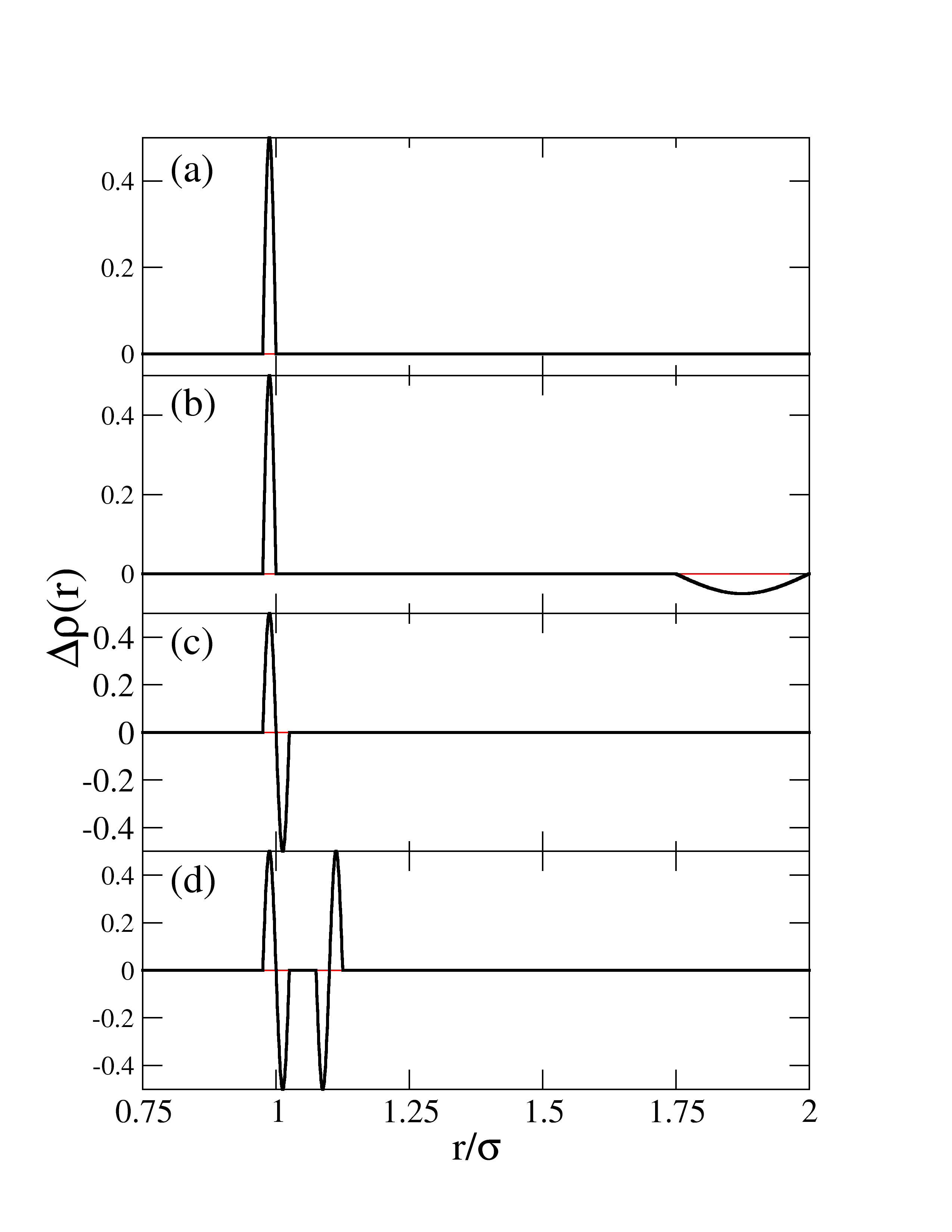
Figure 6: Intuitive picture of allowed and disallowed fluctuations in $\rho(r)$: (a) is not allowed because it violates the global constraint $\int\Delta\rho(r)=0$; (b) satisfies the global constraint but not locality; (c) could correspond, for instance, to a single bond becoming shorter, but this is inconsistent with fixed volume (vanishing first moment—such a change cannot happen in isolation); (d) is allowed—it corresponds, for example, to a single particle being displaced towards one neighbor and away from another. Thus one bond shortens and one lengthens.

It is instructive to repeat the fluctuation mode analysis for a non-strongly correlating liquid, the Dzugutov liquid at $T=0.65$. We do not show the full results here, but they can be summarized as follows. There are two modes which are concentrated at distances less than and around the first minimum of the potential. These have slopes of 5.73 and 5.01 and contribute a total of about 0.35–0.4 to the variances and correlation coefficient. Since the latter is 0.585 at this temperature, these modes account for most of it. There are four more modes which contribute more than 5% to the variances, but the slopes are quite different: -9.34,7.20, 28.43 and -0.67. These four modes all include significant contributions at distances corresponding to the peak in $v(r)$; clearly this extra peak in the potential and the associated peak in the pair-virial $w(r)$ give rise to components in the fluctuations which cannot be related in the manner of an effective inverse power law, even though fluctuations occurring around the minimum can. As a result the overall correlation is rather weak.

II.4 Synthesis: why the effective power-law works even at longer distances

We can apply ideas similar to those used in the crystal analysis to understand why the correlation holds even for modes active at separations larger than the minimum, why the slopes are similar to the effective power-law slopes, and why the effective power law works as well as it does. Recall the essential ingredients of the crystal analysis: the importance of summing over all pairs, the fixed-volume constraint and the increase of magnitude of coefficients of the Taylor expansion with order. These are equally valid here, but now we use them to constrain the allowed deviations in $g(r)$ from its equilibrium value, instead of displacements from a fixed equilibrium configuration. Define the resolved pair-density $\rho(r)$ by

$$\rho(r)\equiv(N/2)4\pi r^{2}\rho g(r).$$ (73)

The requirement that this integrates to the total number of pairs in the system, $\int_{0}^{\infty}\rho(r)dr=N(N-1)/2$, gives a global constraint on fluctuations of $\rho(r)$:

$$\int_{0}^{\infty}\Delta\rho(r)dr=0.$$ (74)

A typical fluctuation will have peaks around the peaks of $g(r)$, but only those near the first peak will significantly affect the potential energy and virial (subsection II.3). We can assume that, for a dense liquid not close to a phase transition, almost any configuration $\Gamma$ may be mapped to a nearby reference configuration $\Gamma_{\textrm{ref}}$ whose RDF is identical with the thermal average $g(r)$. ‘Nearby’ implies that the particle displacements relating the $\Gamma$ and $\Gamma_{\textrm{ref}}$ are small compared to the inter-particle spacing. These displacements define the deviation $\Delta\rho(r)$ of $\rho(r)$ from its equilibrium value. Mapping to $\Gamma_{\textrm{ref}}$ gets around the absence of a unique equilibrium configuration as in the crystal case.

Let us consider what restriction this places on $\Delta\rho(r)$; these are illustrated in Fig. 6. Because the displacements are small, $\Delta\rho(r)$ must be local: a peak in $\Delta\rho(r)$ at some $r$ must be compensated by an opposite peak at a nearby location $r_{\textrm{ref}}$, rather than one far away (thus example (b) in the figure is not allowed)—this corresponds to a bond having length $r$ in the actual configuration and length $r_{\textrm{ref}}$ in $\Gamma_{\textrm{ref}}$ (Fig. 6 (c)). Finally fixed volume implies that a fluctuation cannot involve any substantial change in the mean nearest-neighbor bond length. This may be expressed mathematically as the near vanishing of the first moment of $\Delta\rho(r)$:

$$\int_{\textrm{first peak}}r\Delta\rho(r)dr\cong 0.$$ (75)

Thus, if a particle is displaced towards a neighbor on one side, it is displaced away from a neighbor on the opposite side, thus the resulting fluctuation is expected to look like Fig. 6(d), which is characterized by having vanishing zeroth and first moments. Note that we restrict the integral to the first peak. The principle that fluctuations of $\Delta\rho(r)$ must be local allows us to write a version of Eq. (74) similarly restricted:

$$\int_{\textrm{first peak}}\Delta\rho(r)dr=0$$ (76)

Equations (75) and (76) cannot be literally true, since there must be contributions from fluctuations at whatever cut-off distance is used to define the boundary of the first peak. For instance, there could be a fluctuation such as Fig 6(d) centered just to the right of this cut-off, so that only the first positive part was included in the integrals. We can ignore these contributions if we assume that the potential is truncated and shifted to zero at the boundary, as is standard in practice (although usually at larger distances). Then fluctuations right at the boundary do not contribute to the potential energy. The fact that the only contributions to the integral are at the boundary is a restatement of the locality of fluctuations.

Now we make a Taylor series expansion of $v(r)$ around the maximum $r_{M}$ of the first peak of $g(r)$, using $U=\int_{0}^{\infty}\rho(r)v(r)dr$,

$$\Delta U= \int_{\textrm{first peak}}\Delta\rho(r)\Biggl{(}v(r_{M})+k_{1}(r-r_{M})$$

$$\left.+\frac{1}{2}k_{2}(r-r_{M})^{2}+\ldots\right)\equiv\sum_{p}\frac{k_{p}}{p!}M_{p}.$$ (77)

As for the crystal $k_{p}$ is the $p$th derivative of $v(r)$ at the expansion point ($r_{M}$ here), while $M_{p}$ is the $p$th moment of $\Delta\rho(r)$:

$$M_{p}\equiv\int_{\textrm{first peak}}\Delta\rho(r)(r-r_{M})^{p}dr.$$ (78)

A similar series exists for $W$, with coefficients given by Eq. (27):

$$3\Delta W=\sum_{p}\frac{C_{p}^{W}}{(r_{M})^{p}}M_{p}.$$ (79)

The moments play a role exactly analogous to the sums $S_{p}$ in the analysis of the crystal. The near vanishing of $M_{1}$ corresponds to that of $S_{1}$ in the crystal case, both following from the fixed-volume constraint; as there, it probably holds only to first order in particle displacements (except in one dimension where it is exact), but we have not tried to make a detailed estimate as we did with the crystal. Recalling that the extra contributions to the $M_{2}$ terms will be small anyway, in view of Eqs. (31–32), we simply set $M_{1}=0$, so the two series become (noting that $M_{0}=0$ also)

$$\Delta U =\sum_{p=2}^{\infty}C_{p}^{U}\frac{M_{p}}{r_{M}^{p}}$$

$$3\Delta W =\sum_{p=2}^{\infty}C_{p}^{W}\frac{M_{p}}{r_{M}^{p}}$$ (80)

where the coefficients $C_{p}^{U,W}$ are those defined in Eqs. (26) and (27), but with $r_{M}$ replacing $a_{c}$. The points made in subsection II.2 regarding the relation between the two series are equally valid here. At orders $p=2$ and higher, corresponding coefficients are related by the $n^{(p)}(r_{M})$, which are always all above $a=12$. We expect from dimensional considerations that the variance of $M_{p}$ is proportional to $Nw_{FP}^{2p}$, where $w_{FP}\sim 0.3r_{M}$ is the width of the first peak of $g(r)$. Thus moments of higher order should contribute less, and therefore $M_{2}$ should dominate, implying that the proportionality between $\Delta U$ and $\Delta W$ is essentially $n^{(2)}(r_{M})$. This is in the range 15–24 for $r_{M}$ in the range 1.05$\sigma$–1.15$\sigma$, giving slopes between 5 and 8, similar to those observed in the fluctuation modes. Unlike the low-$T$ limit of the crystal, we cannot assume the fluctuations are particularly localized around $r_{M}$, so it is not surprising that a range of slopes show up. Notice that we do not see arbitrarily high mode slopes corresponding to the divergence of $n^{(2)}(r)$ at the inflection point of the potential. Rather, for modes centered there, the assumption that we can neglect higher moments of the fluctuations no longer holds and there is an interpolation between $n^{(2)}(r)$ and $n^{(3)}(r)$ which is smaller (but still greater than $a=12$).

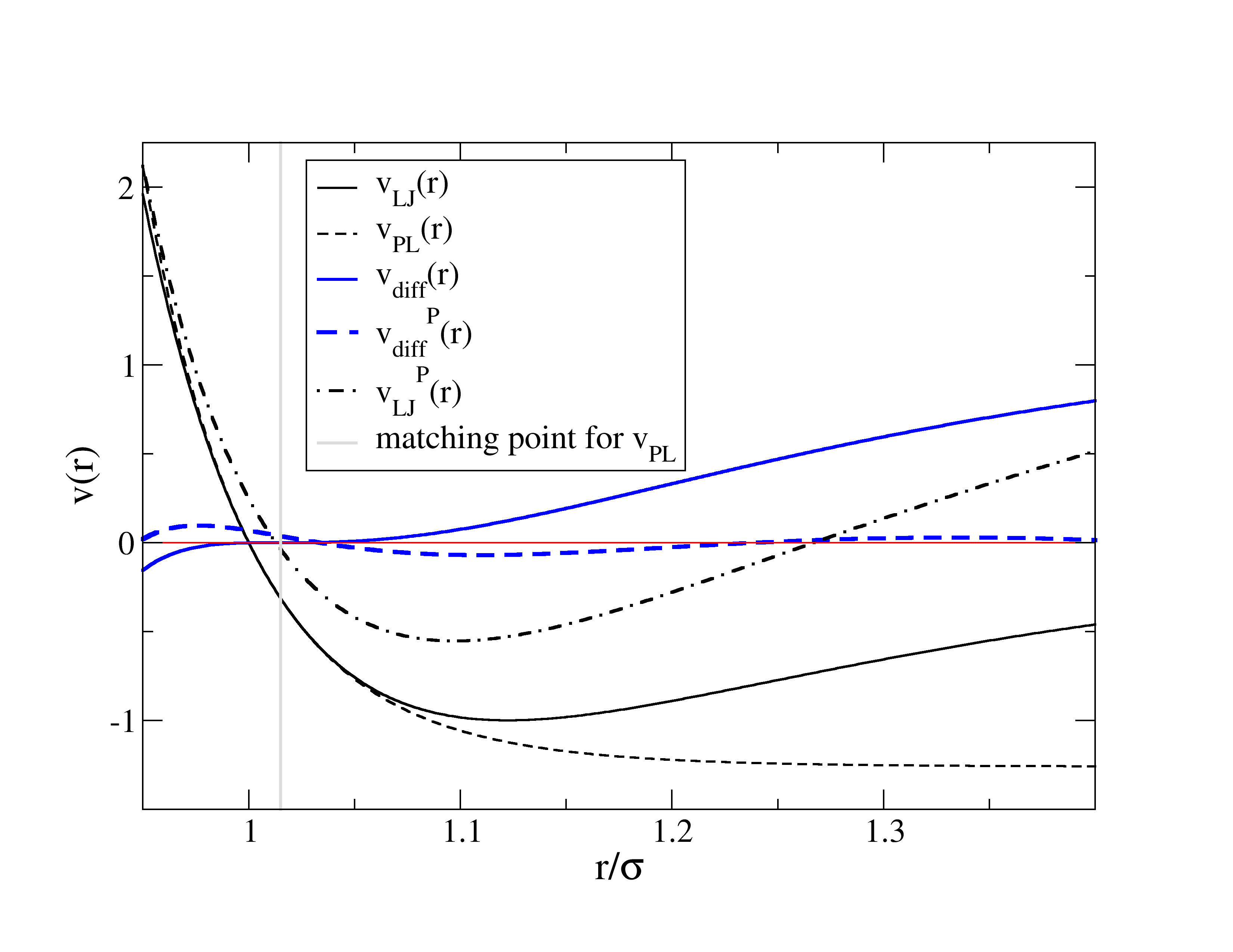
Figure 7: The true potential $v_{LJ}(r)$, the best effective power law $v_{PL}(r)$ (in the sense that the fluctuations in potential energy and virial and reproduced most faithfully), and their difference $v_{\textrm{diff}}(r)$. Also shown are the projected versions $v_{LJ}^{P}(r)$ and $v_{\textrm{diff}}^{P}(r)$ where the constant and linear terms (determined over the interval $0.95\sigma$ to $1.4\sigma$) have been subtracted off. It is the projected functions that should be compared in order to make a statement about the smallness of $v_{\textrm{diff}}(r)$ relative to $v_{LJ}(r)$, since only the projected functions contribute to fluctuations of total potential energy.

We can now understand also why the potential and virial fluctuations, as “reconstructed” using the effective power-law potential (Fig. 3), agree so well with the true fluctuations, even though the fluctuation mode analysis shows that there are significant contributions from distances around and beyond the minimum, well away from the matching point $r=1.015\sigma$. Fig. 7 shows the LJ(12,6) potential, the $n=19.2$ power law (which gave the best fit in subsection II.1), and their difference, $v_{\textrm{diff}}(r)\equiv v_{LJ}(r)-v_{PL}(r)$. The latter is obviously very small and flat near the matching point, but grows significantly in an approximately linear fashion at distances larger than $r\sim 1.05\sigma$. In view of Eqs. (16) and (73), a fluctuation of $U_{\textrm{diff}}$ can be written as

$$\Delta U_{\textrm{diff}}=\int_{0}^{\infty}v_{\textrm{diff}}(r)\Delta\rho(r)dr,$$ (81)

which has the form of an inner product of functions. Vanishing fluctuations of $U_{\textrm{diff}}$ follows if either (1) $v_{\textrm{diff}}$ is identically zero, or (2) it is non-zero, but orthogonal to the space of allowed $\Delta\rho(r)$. Given that $v_{\textrm{diff}}$ is not particularly small except close to the matching point (see Fig. 7), the fact that $U_{\textrm{diff}}$ fluctuations are relatively small even though they are associated with distances away from the matching point indicates that point (2) must hold approximately. Since allowed $\Delta\rho(r)$ functions are those with no constant or linear term (see Eqs. (74) and (75)), functions orthogonal to these are those with only a constant and linear term: $f(r)=Cf_{0}(r)+Df_{1}(r)$ where $f_{0}(r)$ is a constant function and $f_{1}(r)$ is a linear function with zero mean over the range of interest. It is clear in Fig. 7 that $v_{\textrm{diff}}$ is not exactly of this form, but it can be well approximated by such a function. This approximation can be checked by standard methods of the linear algebra of function spaces. First we choose a range $(r_{1},r_{2})$ over which functions are to be defined. For purposes this should include the range of significant contributions to $W$ and $U$ (Fig. 5). We choose $r_{1}=0.95\sigma$ and $r_{2}=1.4\sigma$. The normalized, mutually orthogonal basis vectors $f_{0}(r)$ and $f_{1}(r)$ are then given by

$$f_{0}(r) =1/\sqrt{r_{2}-r_{1}}$$

$$f_{1}(r) =\sqrt{\frac{12}{(r_{2}-r_{1})^{3}}}(r-(r_{1}+r_{2})/2).$$ (82)

The part of $v_{\textrm{diff}}(r)$ which is spanned by these basis functions is $v_{0}f_{0}+v_{1}f_{1}$ where $v_{i}\equiv\int_{r_{1}}^{r_{2}}f_{i}(r)v_{\textrm{diff}}(r)dr$ is the inner product of $v_{\textrm{diff}}(r)$ and the corresponding basis vector. We define $v_{\textrm{diff}}^{P}(r)$ as the part of $v_{\textrm{diff}}(r)$ projected onto the space of allowed functions:

$$v_{\textrm{diff}}^{P}(r)=v_{\textrm{diff}}(r)-v_{0}f_{0}(r)-v_{1}f_{1}(r).$$ (83)

This function is also plotted in Fig. 7, where it can be seen that it is certainly small compared to $v_{\textrm{diff}}(r)$ itself. More importantly, it is also small compared to the projected part of $v_{LJ}(r)$, $v_{LJ}^{P}(r)$, defined analogously, because it is this that explains why the fluctuations of $U_{\textrm{diff}}$ are small compared to those of $U_{LJ}$ (or equivalently $U_{PL}$). This may be quantified by noting that the ratio of their norms is $0.09$, which indicates how orthogonal $v_{\textrm{diff}}(r)$ is to the space of allowed $\Delta\rho(r)$. If we projected out only the constant term from $v_{\textrm{diff}}(r)$ and $v_{LJ}^{P}(r)$ (the a priori more obvious way to compare the size of two functions) the ratio of norms would be $0.50$, and it would not be obvious why $v_{PL}$ does as good a job as it does. Thus, again, constant volume constraint, implying Eq. (75), is important.

The above discussion applies equally well to the virial. We can now write a more accurate approximate expression for $v_{LJ}(r)$, which we call the “extended effective power-law approximation”:

$$v_{LJ}(r)\simeq Ar^{-n}+B+Cr,$$ (84)

where $A$, $B$ and $C$ are constants. The associated pair virial ($w(r)\equiv rv^{\prime}(r)$) is then

$$w_{LJ}(r)\simeq-nAr^{-n}+Cr,$$ (85)

which has the same form. In both cases the term $Cr$ contributes to the mean value but not the fluctuations, because $\int r\rho(r)dr$ is non-zero, while $\int r\Delta\rho(r)dr=0$ for those $\Delta\rho(r)$ which are allowed at fixed volume. Note also the contribution to the mean values from $Cr$ will depend on volume because $g(r)$, and hence $\rho(r)$, do. Thus we can see that although there are significant contributions to fluctuations away from the matching point where the power law fits the true potential well, these are essentially equal for both the power-law and the true potential, because the difference between the two potentials in this region is almost orthogonal to the allowed fluctuations in $\rho(r)$. This also explains why the fluctuation only holds at fixed volume (which would not be explained by the assumption that short-distance encounters dominate the fluctuations).

The extended power-law approximation, determined empirically by the projection procedure, provides an alternative way to understand why the effective exponent $n^{(1)}$ evaluated at $r\sim\sigma$ agrees well with $n^{(2)}$ evaluated around the minimum $r_{m}$. For the extended effective power-law approximate, Eq. (84) we get

$$n^{(1)}(r) =\frac{-n(n+1)Ar^{-(n+1)}}{-nAr^{-(n+1)}+C}-1$$

$$n^{(2)}(r) =\frac{n(n+1)(n+2)Ar^{-(n+2)}}{n(n+1)Ar^{-(n+2)}}-2=n;$$ (86)

Note that $n^{(2)}(r)$ is constant, and equal to the exponent $n$ of the power-law while $n^{(1)}(r)$ only approaches $n$ when $r$ is small enough that the $C$ in the denominator can be neglected (for the true potential $n^{(2)}(r)$ increases with $r$ and eventually diverges, see Fig. 1). This emphasizes the greater usefulness of $n^{(2)}$ in identifying the effective power-law exponent. Recall also that our analysis earlier in this section indicates that $n^{(2)}(r)$, involving the second and third derivatives of $v(r)$ near its minimum, is more fundamentally the cause of the $W,U$ correlations, explaining something like 80% of the correlation in the liquid phase and over 99% in the crystal phase. The fact that Eq. (84) is a good approximation for the Lennard-Jones potential pushes the correlation to over 90% also in the liquid phase.

To summarize the last two subsections, we have shown here that the source of the fluctuations is indeed pair-separations within the first peak, although only a relatively small fraction of the variances come from the short-$r$ region where the approximation of the pair potential by a power law is truly valid. We have also seen how the Taylor-series analysis (which involves the crucial step of taking a sum over all pairs) may be extended to cover the whole first peak area, with all terms giving roughly the same effective slope, given essentially by the second-order effective exponent: $\gamma\sim n^{(2)}(r_{m})/3$. The fact that this matches the first-order effective exponent at the shorter distance $r\sim\sigma$ is equivalent to the extended effective power-law approximation (Eq. (84)), which given constant volume is what justifies the replacement of the potential by a power law (empirically demonstrated in Fig. 3).

III Some consequences of strong pressure-energy correlations

This section gives examples of consequences of strong pressure-energy correlations. The purpose is show that these are important, whenever present. Clearly, more work needs to be done to identify and understand all consequences of strong pressure energy-correlations.

III.1 Measurable consequences of instantaneous $W,U$-correlations

The observation of strong $W,U$ correlations is of limited interest if it can only ever be observed in simulations. How can we make a comparison with experiment? In general, fluctuations of dynamical variables are related to thermodynamic response functions,Landau and Lifshitz (1980); Hansen and McDonald (1986); Reichl (1998) for example those of $U$ are related to the configurational part of the specific heat, $C_{V}^{\textrm{conf}}$. The latter is obtained by subtracting off the appropriate kinetic term, which for a monatomic system such as Argon is $3Nk_{B}/2$. The virial fluctuations, however, although related to the bulk modulus, are not directly accessible, because of another term that appears in the equation, the so-called hypervirial, which is not a thermodynamic quantity.Allen and Tildesley (1987) Fortunately this difficulty can be handled.

Everything in this section refers to the NVT ensemble. First we define the various response functions and configurational counterparts, the isothermal bulk modulus $K_{T}$, $C_{V}$, and the “pressure coefficient”, $\beta_{V}$:

$$\begin{array}[]{rlrl}K_{T}&\equiv-V\left(\frac{\partial\langle p\rangle}{\partial V}\right)_{T},&K_{T}^{\textrm{conf}}&\equiv K_{T}-\frac{Nk_{B}T}{V}\\ C_{V}&\equiv\left(\frac{\partial E}{\partial T}\right)_{V},&C_{V}^{\textrm{conf}}&\equiv C_{V}-\frac{3}{2}Nk_{B}\\ \beta_{V}&\equiv\left(\frac{\partial\langle p\rangle}{\partial T}\right)_{V},&\beta_{V}^{\textrm{conf}}&\equiv\beta_{V}-\frac{Nk_{B}}{V}\\ &&p^{\textrm{conf}}&\equiv p-\frac{Nk_{B}T}{V}=\frac{W}{V}.\end{array}$$ (87)

We also define $c_{V}\equiv C_{V}/V$. The following fluctuation formulas are standard (see for example Ref. Allen and Tildesley, 1987)

$$\frac{\langle(\Delta W)^{2}\rangle}{k_{B}TV} =\frac{Nk_{B}T}{V}+\frac{\langle W\rangle}{V}-K_{T}+\frac{\langle X\rangle}{V}$$ (88)

$$\frac{\langle(\Delta U)^{2}\rangle}{k_{B}T^{2}} =C_{V}-\frac{3}{2}Nk_{B}=C_{V}^{\textrm{conf}}$$ (89)

$$\frac{\langle\Delta U\Delta W\rangle}{k_{B}T^{2}} =V\beta_{V}-Nk_{B}=V\beta_{V}^{\textrm{conf}}.$$ (90)

Here $X$ is the so-called “hypervirial”, which gives the change of virial upon an instantaneous volumetric scaling of positions. It is not a thermodynamic quantity and cannot be determined experimentally, although it is easy to compute in simulations. For a pair potential $v(r)$, $X$ is a pair-sum,

$$X=\sum_{\textrm{pairs}}x(r)/9$$ (91)

where $x(r)=rw^{\prime}(r)$. If we use the extended effective power-law approximation (including the linear term) discussed in the last section, then from Eq. (85) we get $x(r)\simeq n^{2}Ar^{-n}+Cr$. Summing over all pairs, and recalling that when the volume is fixed the $Cr$ term gives a constant, we have a relation between the total virial and total hypervirial,

$$X=(n/3)W+\textrm{constant}.$$ (92)

This constant survives, of course, when we take the thermal average $\langle X\rangle$, as do the corresponding constants in $\langle U\rangle$, $\langle W\rangle$. To get rid of these constants one possibility would be to take derivatives with respect to $T$, but this can be problematic when analyzing experimental data. Instead we simply compare quantities at any temperature to those at some reference temperature $T_{\textrm{ref}}$; this effectively subtracts off the unknown constants. Taking first the square of the correlation coefficient, we have

$$R^{2}=\frac{(\langle\Delta U\Delta W\rangle)^{2}}{\langle(\Delta U)^{2}\rangle\langle(\Delta W)^{2}\rangle},$$ (93)

which implies

$$R^{2}\frac{\langle(\Delta W)^{2}\rangle}{k_{B}TV}=\frac{1}{k_{B}TV}\frac{(\langle\Delta U\Delta W\rangle)^{2}}{\langle(\Delta U)^{2}\rangle}.$$ (94)

Inserting the fluctuation formulas Eqs. (88) and (90) gives

$$R^{2}(\langle p\rangle-K_{T}+\frac{\langle X\rangle}{V})= \frac{1}{k_{B}TV}\frac{(k_{B}T^{2}V\beta_{V}^{\textrm{conf}})^{2}}{k_{B}T^{2}C_{V}^{\textrm{conf}}}$$ (95)

$$=T\frac{(\beta_{V}^{\textrm{conf}})^{2}}{c_{V}^{\textrm{conf}}}.$$ (96)

Defining quantities $\tilde{A}\equiv\langle p\rangle-K_{T}+\langle X\rangle/V$ and $B\equiv T(\beta_{V}^{\textrm{conf}})^{2}/c_{V}^{\textrm{conf}}$ (the reason for the tilde on $A$ will become clear), we have $R^{2}\tilde{A}=B$. This is an exact relation. To deal with the hypervirial we first take differences with the quantities at $T_{\textrm{ref}}$, assuming that the variation of $R$ is much smaller than the $\tilde{A}$ and $B$ variations:

$$R^{2}(\tilde{A}-\tilde{A}_{\textrm{ref}})=B-B_{\textrm{ref}}$$ (97)

where $\tilde{A}_{\textrm{ref}}=\tilde{A}(T_{\textrm{ref}})$, etc. $\tilde{A}-\tilde{A}_{\textrm{ref}}$ written out explicitly is

$$\tilde{A}-\tilde{A}_{\textrm{ref}}=(\langle p\rangle-K_{T})-(\langle p\rangle_{\textrm{ref}}-{K_{T}}_{\textrm{ref}})+\frac{\langle X\rangle-\langle X\rangle_{\textrm{ref}}}{V}$$ (98)

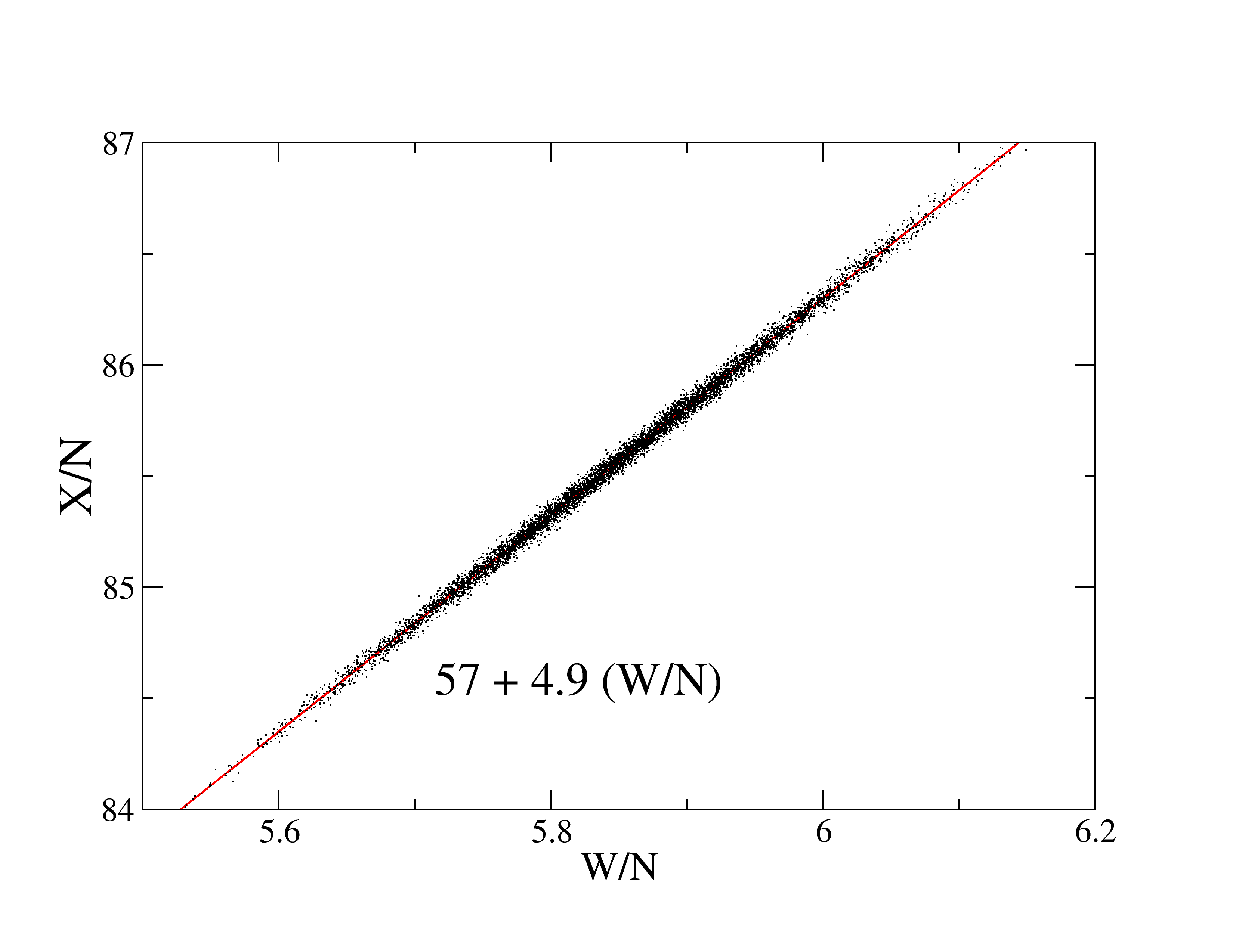
Figure 8: Scatter-plot of instantaneous virial and hypervirial (in dimensionless units) for a SCLJ system at $\rho=1.0,T=0.80$ (NVE). The correlation coefficient between these quantities is 0.998. The hypervirial is the main contribution to the configurational part of the bulk modulus; it gives (after dividing by volume) the change of virial for a given relative change in volume. The sizeable constant term in the linear fit shows that Eq. (92) is a poor approximation. The slope is 4.9, about 10% smaller than $\gamma\sim 5.4$ for this state point. The difference reflects the limit of the validity of the power-law description–in fact a more detailed analysis shows that the relation between $W$ and $X$ is dominated by $n^{(3)}(r)$, which is smaller than $n^{(2)}(r)$ (Fig. 1).

Next we use the power-law approximation to replace $\langle X\rangle-\langle X_{\textrm{ref}}\rangle$ with $(n/3)(\langle W\rangle-\langle W_{\textrm{ref}}\rangle)$. This is the crucial point: Whereas it is often not a good approximation that $\langle X\rangle=(n/3)\langle W\rangle$ due to the unknown additive constants discussed above, subtracting two state points considers changes of $\langle X\rangle$ and $\langle W\rangle$ with temperature. Recall from section III B of Paper I that the changes in mean-values $\Delta\langle W\rangle$ and $\Delta\langle X\rangle$ between (nearby) temperatures are related as the linear regression of the fluctuations of those quantities at one (nearby or intermediate) temperature. The linear relation between subtracted mean values holds if the instantaneous $W$ and $X$ are strongly correlated in the region of interest. The latter is confirmed by our simulations; indeed the correlation of instantaneous values of $X$ and $W$ is even stronger than for $W$ and $U$, with approximately the same slope (Fig. 8). Thus Eq. (98) becomes

$$\tilde{A}-\tilde{A}_{\textrm{ref}} \simeq(\langle p\rangle-K_{T})-(\langle p\rangle_{\textrm{ref}}-{K_{T}}_{\textrm{ref}})+\frac{n}{3}\frac{\langle W\rangle-\langle W\rangle_{\textrm{ref}}}{V}$$ (99)

$$=A-A_{\textrm{ref}}$$ (100)

where $A\equiv p-K_{T}+(n/3)(\langle W\rangle/V)$ (no tilde) contains quantities which are all directly accessible to experiment, except for the effective power-law exponent $n$. This can be obtained by noting that if there were perfect correlation, one could interchange $\Delta W$ and $(n/3)\Delta U$; thus

$$\frac{\beta_{V}^{\textrm{conf}}}{C_{V}^{\textrm{conf}}/V}=\frac{\beta_{V}^{\textrm{conf}}}{c_{V}^{\textrm{conf}}}=\frac{\langle\Delta U\Delta W\rangle}{\langle(\Delta U)^{2}\rangle}=\frac{n}{3}$$ (101)

which gives for $A$

$$A=\langle p\rangle-K_{T}+\frac{\langle p\rangle^{\textrm{conf}}\beta_{V}^{\textrm{conf}}}{c_{V}^{\textrm{conf}}}.$$ (102)

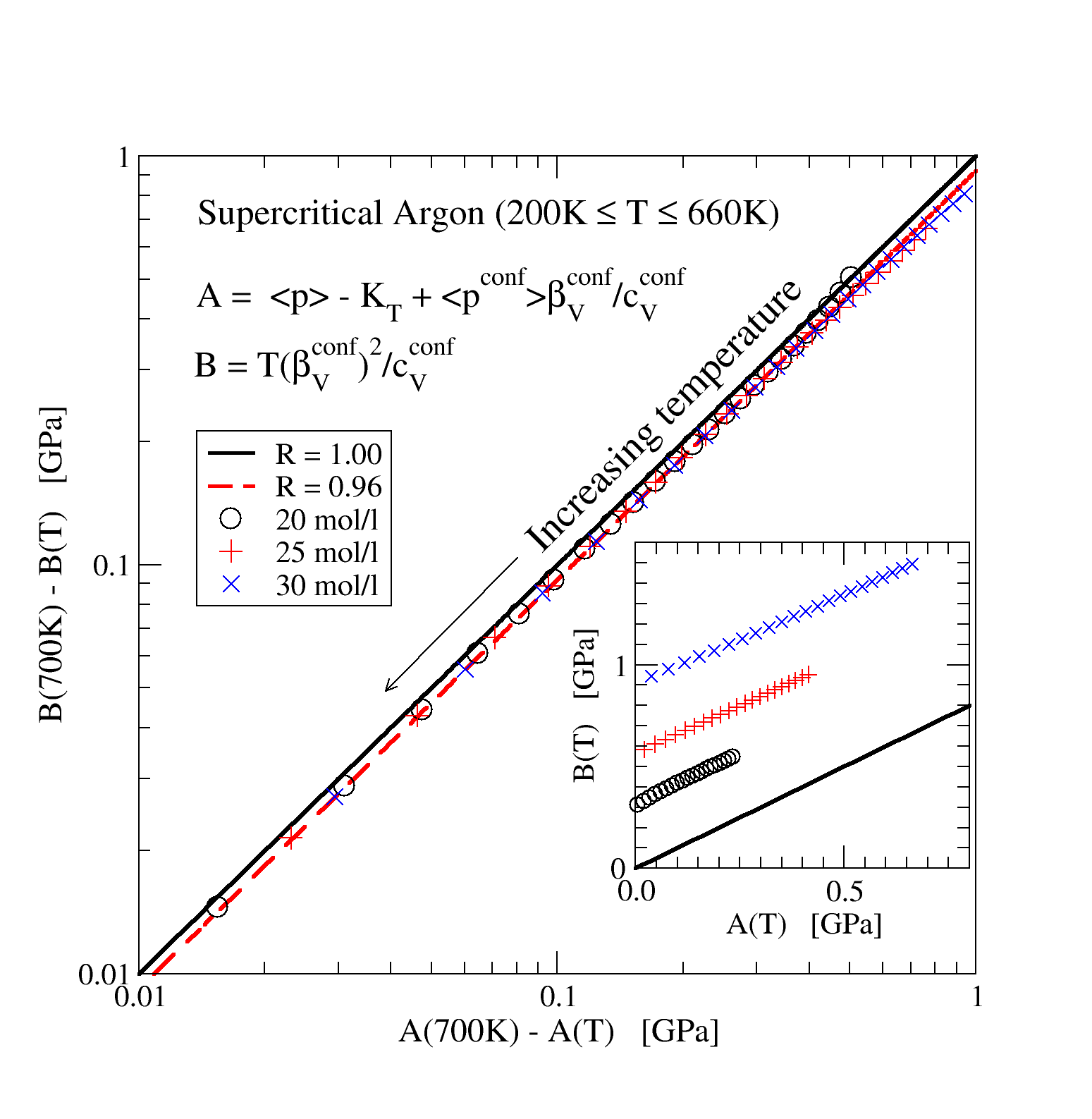
Figure 9: (Color online) Data from the NIST databaseLemmon et al. (2005) for supercritical Argon at three different densities covering the temperature range 200K-660K showing a strong virial-potential energy correlation ($R=0.96$) [reproduced from Ref. Pedersen et al., 2008a]. Here $K_{T}\equiv-V(\partial\langle p\rangle/\partial V)_{T}$, $p^{\textrm{conf}}\equiv p-Nk_{B}T/V=W/V$ $\beta_{V}^{\textrm{conf}}\equiv(\partial\langle p\rangle/\partial T)_{V}-Nk_{B}/V$, and $c_{V}^{\textrm{conf}}\equiv C_{V}/V-(3/2)Nk_{B}/V$ The diagonal line corresponds to perfect correlation. The inset shows “unsubtracted” values for $A$ and $B$; the fact that the data do not fall on the solid line indicates that a power-law description does not hold for the full thermodynamics.

Thus to compare with experiment one should plot $B-B_{\textrm{ref}}$ against $A-A_{\textrm{ref}}$; the prediction, in the case of near perfect correlation, $R^{2}\simeq 1$, is a straight line with slope close to unity. Fig. 9 shows data for Argon for $T$ between 200K and 660K. Argon was chosen because as a monatomic system there are no rotational or vibrational modes contributing to the heat capacity and it is therefore straightforward to subtract off the kinetic part. Also we restrict to relatively high temperature to avoid quantum effects. The correlation coefficient $R$ given as the square root of the slope of a linear fit is 0.96. Note that the assumed constancy of $R$ is confirmed (going to lower temperatures there are increasingly large deviations). The importance of subtracting from a reference state point is highlighted by the inset, which shows that $A(T)=B(T)$ does not hold: There is a correlation in the fluctuations which is not present in the full equation of state.Pedersen et al. (2008a)

III.2 Time averaging: Pressure-energy correlations in highly viscous liquids

We have observed and discussed in paper I that when volume is held constant, the correlations tend to become more perfect with increasing $T$, while along an isobar (considering still fixed-volume simulations, choosing the volume to give a prescribed average pressure), they become more perfect with decreasing $T$. This fact makes the presence of correlations highly relevant for the physics of highly viscous liquids approaching the glass transition. Basic questions such as the origins of non-exponential relaxations and non-Arrhenius temperature dependence are still vigorously debated in this field of research.Kauzmann (1948); Brawer (1985); Angell et al. (2000); Dyre (2006) Instantaneous correlations of the kind discussed in this work would seem to be relevant only to the high frequency properties of a highly viscous liquid; their relevance to the long time scales on which structural relaxation occurs follows from the separation of time scales as explained below.

A question that is not actively debated in this research field (but see, e.g., Refs. Schmelzer and Gutzow, 2006; Bailey et al., 2008b; Ellegaard et al., 2007), is whether a single parameter is enough to describe a highly viscous liquid. The consensus for more than 30 years is that with few exceptions these liquids require more than just one parameter, a conclusion scarcely surprising given their complexity. The meaning of “having a single parameter” can be understood as follows. Following a sudden change in volume, both pressure and energy relax to their equilibrium values over a time scale of minutes or even hours, sufficiently close to the glass transition. If a single parameter governs the internal relaxation of the liquid, then both pressure and energy relax with the same time scale, and in fact the normalized relaxation functions are identical.Bailey et al. (2008b); Ellegaard et al. (2007) This behavior can be expressed in the frequency domain, as a certain quantity, the dynamic Prigogine-Defay ratio, being equal to unity.Ellegaard et al. (2007) A key feature of highly viscous liquids is the separation of time scales between the slow structural (“alpha”) relaxation (up to of order seconds) and the very short times (of order picoseconds) characterizing the vibrational motion of the molecules. This separation allows a more direct experimental consequence of $W,U$ correlations than that described in the previous subsection: Suppose a highly viscous liquid has perfectly correlated $W,U$ fluctuations. When $W$ and $U$ are time-averaged over, say, one tenth of the alpha relaxation time $\tau_{\alpha}$,Pedersen et al. (2008b) they still correlate 100%. Since the kinetic contribution to pressure is fast, its time-average over $\tau_{\alpha}/10$ is just its thermal average, and thus the time-averaged pressure equals the time-average of $W/V$ plus a constant. Similarly, the time-averaged energy equals the time-averaged potential energy plus a constant. Thus the fluctuations of the time-averaged $W$ and $U$ equal the slowly fluctuating parts of pressure and energy, so these slow parts will also correlate 100% in their fluctuations. In this way we get from the non-observable quantities $W$ and $U$ to the observable ones $E$ and $p$ (we similarly averaged to observe the correlation in the SQW system in Paper I). The upper part of Fig. 10 shows normalized fluctuations of energy and pressure for the commonly studied Kob-Andersen binary Lennard-Jones systemKob and Andersen (1994) (referred to as KABLJ in Paper I), time-averaged over one tenth of $\tau_{\alpha}$. In the lower part we show the dynamic Prigogine-Defay ratio,Ellegaard et al. (2007) which in the NVT ensemble is defined as follows:

$$\Lambda_{TV}(\omega)\equiv-\frac{c_{V}^{\prime\prime}(\omega)(1/\kappa_{T}(\omega))^{\prime\prime}}{T\left[\beta_{V}^{\prime\prime}(\omega)\right]^{2}};$$ (103)

here $\kappa_{T}=1/K_{T}$ is the isothermal compressibility and ^′′ denotes the imaginary part of the complex frequency dependent response function. A way to interpret this quantity can be found by considering the fluctuation-dissipation theorem expressions for the response functions. For example the frequency-dependent constant-volume specific heat $c_{V}(\omega)$ is givenNielsen and Dyre (1996) by

$$c_{V}(\omega)=\frac{\langle(\Delta E)^{2}\rangle}{k_{B}T^{2}}-\frac{i\omega}{k_{B}T^{2}}\int_{0}^{\infty}{\langle\Delta E(0)\Delta E(t)\rangle\exp(-i\omega t)}dt$$ (104)

where $E$ is the total energy. Taking the imaginary part we have

$$c_{V}^{\prime\prime}(\omega)=-\frac{\omega}{k_{B}T^{2}}(\mathcal{L}\{\langle\Delta E(0)\Delta E(t)\rangle\})^{\prime}$$ (105)

where we use $\mathcal{L}$ to represent Laplace transformation. Similarly

$$(1/\kappa_{T})^{\prime\prime}(\omega)=\frac{\omega V}{k_{B}T}(\mathcal{L}\{\langle\Delta p(0)\Delta p(t)\rangle\})^{\prime}$$ (106)

and

$$\beta_{V}^{\prime\prime}(\omega)=-\frac{\omega}{k_{B}T^{2}}(\mathcal{L}\{\langle\Delta E(0)\Delta p(t)\rangle\})^{\prime}$$ (107)

Forming the Prigogine-Defay ratio then gives, after cancelling factors of $k_{B}$, $T$, $V$, and $\omega$,

$$\Lambda_{TV}(\omega)=\frac{(\mathcal{L}\{\langle\Delta E(0)\Delta E(t)\rangle\})^{\prime}(\mathcal{L}\{\langle\Delta p(0)\Delta p(t)\rangle\})^{\prime}}{(\mathcal{L}\{\langle\Delta E(0)\Delta p(t)\rangle\})^{\prime 2}}.$$ (108)

We can see that the right-hand side has a similar structure to a correlation coefficient, if we take the inverse square root. So in a loose sense the dynamic Prigogine-Defay ratio can be thought of as the inverse square of a correlation coefficient, referred to a particular time scale. This gives an intuitive reason for why it is in general greater or equal to unity, with equality only achieved in the case of perfect correlation.Ellegaard et al. (2007) The lower panel of Fig. 10 shows this quantity for a range of frequencies for the KABLJ system. It clearly approaches one at low frequencies, and stays within 20% of one in the main relaxation region. In the sense above, this corresponds to $R>0.9$, or strongly correlation.

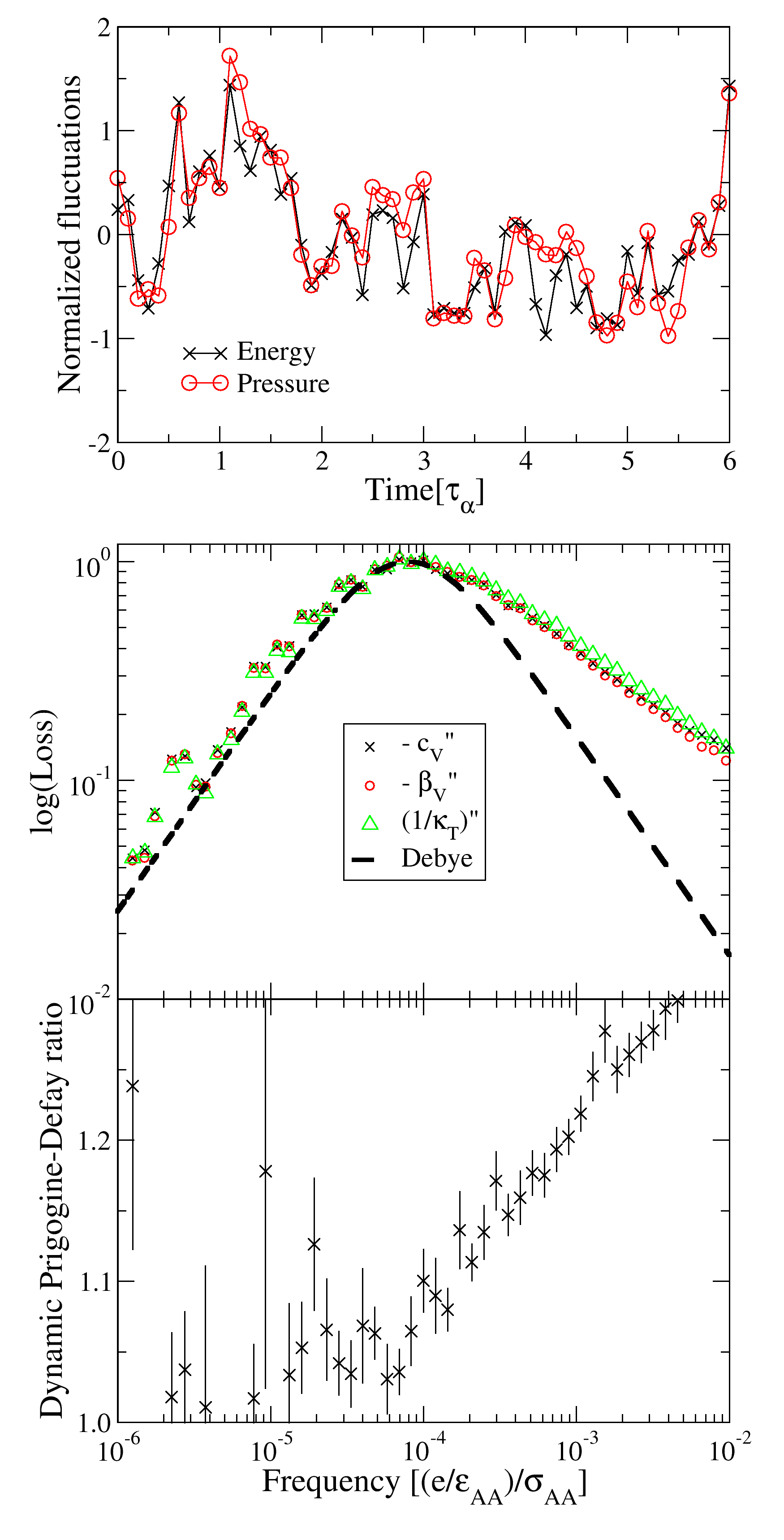
Figure 10: (Color online) Upper panel, time-averaged (over $\tau_{\alpha}/10$, where $\tau_{\alpha}$ is the structural relaxation time), normalized fluctuations of $E$ and $p$ in NVT simulations of the Kob-AndersenKob and Andersen (1994) binary Lennard-Jones (KABLJ) system, plotted against time in units of $\tau_{\alpha}\sim 10^{3}\sigma_{AA}\sqrt{m/\epsilon_{AA}}$. The density was 1.2$\sigma_{AA}^{-3}$, and the temperature $0.474\epsilon_{AA}$. Middle panel, imaginary parts of the three response functions $-c_{v}(\omega)$, $-\beta_{V}(\omega)$ and $1/\kappa_{T}(\omega)$, scaled to the maximum value. Lower panel, dynamic Prigogine-Defay ratio for the same simulation. The approach towards unity at frequencies smaller than the loss-peak frequency ($\sim 1/\tau_{\alpha}$) is exactly equivalent to the correlation between time-averaged quantities shown in the upper panel [reproduced from Ref. Pedersen et al., 2008b].

The line of reasoning presented here opens for a new way of utilizing computer simulations to understand ultraviscous liquids. Present-day computers are barely able to simulate one microsecond of real-time dynamics, making it difficult to predict the behavior of liquids approaching the laboratory glass transition. We find that pressure-energy correlations are almost independent of viscosity, however, which makes it possible to make predictions regarding the relaxation properties even in the second or hour range of characteristic times. Thus if a glass-forming liquid at high temperatures (low viscosity) has very strong pressure-energy correlations ($R\sim 1$), its eight thermoviscoelastic response functions at ultraviscous conditions may basically be expressed in terms of just one, irrespective of temperature (or viscosity).

III.3 Aging and energy landscapes

We now discuss the significance of the present results for the interesting results reported in 2002 by Mossa et al,Mossa et al. (2002) who studied the inherent states visited by the Lewis-Wahnström modelLewis and Wahnström (1994) of the glass-forming liquid orthoterphenyl (OTP) during aging, i.e., the approach to equilibrium. An inherent state (IS) is a local minimum of the so-called potential energy landscape (PEL) to which a given configuration is mapped by steepest-descent minimization.Goldstein (1969); Stillinger (1995) The PEL formalism involves modeling the distributions and averages of properties of the IS in the hope of achieving a compact description of the thermodynamics of glass-forming liquids.Sciortino (2005); Heuer (2008) The thesis of Ref. Mossa et al., 2002 and of the previous work La Nave et al. (2002) is that an equation of state can be derived using this formalism which is valid even for non-equilibrium situations. This involves including an extra parameter, namely the average IS (potential) energy, $\langle e_{IS}\rangle$, so that the equation of state takes the form

$$p(T,V,\langle e_{IS}\rangle)=p_{IS}(\langle e_{IS}\rangle,V)+p_{\textrm{vib}}(T,V,\langle e_{IS}\rangle)$$ (109)

where $p_{IS}$ is the ensemble averaged inherent state pressure—for a given configuration it is the pressure of the corresponding inherent state—and $p_{\textrm{vib}}\equiv p-p_{IS}$. The usefulness of splitting in this way lies in the fact that $p_{IS}$ does not explicitly depend on $T$.

In equilibrium $\langle e_{IS}\rangle$ is determined by $V$ and $T$. The conclusion of Ref. Mossa et al., 2002 is that knowledge of $\langle e_{IS}\rangle$ in non-equilibrium situations is enough to predict the corresponding pressure (given also $T$ and $V$). This was based on extensive simulations of various aging schedules. Thus the authors conclude that the inherent states visited by the system while out of equilibrium, must be in some sense the “same” ones sampled during equilibrium conditions. “Same” is effectively defined by their results that averages of various inherent state properties ($V$, $e_{IS}$, $p_{IS}$, as well as a measure of the IS curvature) are all related to each other the same way under non-equilibrium conditions as under equilibrium conditions. It was similarly found that the volume could be determined from $\langle e_{IS}\rangle$ following a pressure jump in a pressure-controlled simulation. On the other hand, subsequent work by the same group found that this was not at all possible for glassy water during compression/decompression cycles. Giovambattista et al. (2003)

Now, our results (Paper I) for the same OTP model show that it is a strongly correlating liquid. Thus we expect a general correlation between individual, not just average, values of $p_{IS}$, the inherent state pressure (which lacks a kinetic term and therefore equals the inherent state virial divided by volume) and $e_{IS}$, for a given volume. Therefore, for any given collection of inherent states with the same volume—not just equilibrium ensembles—the mean values of $U$ and $W$ will fall on the same straight line as the instantaneous values. Note that this would not hold if the correlation was non-linear. Correspondingly for given $p_{IS}$, there is a general correlation between individual values of $e_{IS}$ and $V$. In fact, any two of these quantities determine the third with high accuracy, and this is true at the level of individual configurations, including inherent states.

To see how this works for cases involving fixed volume, we write the total (instantaneous) pressure as a sum of an inherent state part, which involves the the virial at the corresponding inherent state, plus a term involving the difference of the true virial from the inherent state virial, plus the kinetic term:

$$p=\frac{W_{IS}}{V}+\frac{W-W_{IS}}{V}+\frac{Nk_{B}T}{V}.$$ (110)

The first term is linearly related to the inherent state energy for a strongly correlating liquid. Moreover, the difference term is similarly expressed in terms of the corresponding energy difference, $W-W_{IS}=\gamma(U-e_{IS})$. Taking averages over the (possibly non-equilibrium, although we assume equilibrium within a given potential energy basin) ensemble, we expect that $\langle U-e_{IS}\rangle$ depends only on $T$ and $V$ (a slight $e_{IS}$ dependence can appear in $\gamma$ since this is slightly state-point dependent). Thus it follows that $p$ can be reconstructed from a knowledge of (average) $e_{IS}$, $V$ and $T$, without any assumptions about the nature of the inherent states visited. In particular, no conclusion can be drawn regarding the latter. The failure of the pressure reconstruction in the case of water Giovambattista et al. (2003) is not surprising, since water models are generally not strongly correlating (which as we saw in Paper I is linked to the existence of the density maximum).

III.4 Biomembranes

A completely different area of relevance for the type of correlations reported here relates to recent work of Heimburg and Jackson,Heimburg and Jackson (2005) who have proposed a controversial new theory of nerve signal propagation. Based on experiment and theory they suggest that a nerve signal is not primarily electrical, but a soliton sound-wave.Heimburg and Jackson (2007) Among other things this theory explains how anaesthesia works (and why one can dope people with the inert gas Xenon): Anaesthesia works simply by a freezing-point depression that changes the membrane phase transition temperature and affects its ability to carry the soliton sound wave. A crucial ingredient of the theory is the postulate of proportionality between volume and enthalpy of microstates, i.e., that their thermal equilibrium fluctuations should correlate perfectly. This should apply even through the first-order membrane melting transition. The theory was justified in part from previous experiments by Heimburg showing proportionality between compressibility and specific heat through the phase transition.Ebel et al. (2001) The postulated correlation—including the claim that is survives a first-order phase transition—fits precisely the pattern found in our liquid simulations.

Table 3: Data from NpT simulations of fully hydrated phospholipid membranes of 1,2-Dimyristoyl-sn-Glycero-3-Phosphocholine (DMPC), 1,2-Dimyristoyl-sn-Glycero-3-Phospho-L-Serine with sodium as counter ion (DMPS-Na), hydrated DMPS (DMPSH), and 1,2-Dipalmitoyl-sn-Glycero-3-Phosphocholine (DPPC).Pedersen et al. (2008c); Pedersen et al. (2009) The columns list temperature, correlation coefficient between volume and energy, average lateral area per lipid, simulation time in equilibrium, and total simulation time.

	$T$ [K]	$R_{EV}$	$A_{lip}$ [Å2]	$t$ [ns]	$t_{tot}$ [ns]
DMPC	310	0.885	53.1	60	114
DMPC	330	0.806	59.0	50	87
DMPS-Na	340	0.835	45.0	22	80
DPPC	325	0.866	67.3	13	180

By re-examining existing simulation dataPedersen et al. (2006, 2007) as well as carrying out extensive new simulations,Pedersen et al. (2008c) we have investigated whether the correlations are also found in several model membrane systems, five of which are listed in Table 3. The simulations involved a layer of phospholipid membrane surrounded by water, in the $L_{\alpha}$ phase (that is, at temperatures above the transition to the gel-state), at constant $p$ and $T$. When $p$, rather than $V$, is constant, the relevant quantities that may correlate are energy and volume. As with viscous liquids (subsection III.2) and the square well system (Paper I), time-averaging is necessary for a correlation to emerge, where now

$$\Delta\bar{E(t)}\simeq\gamma^{vol}\Delta\bar{V(t)}$$ (111)

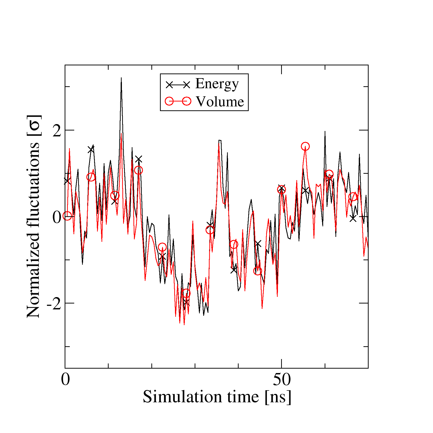
Figure 11: (color online) Normalized fluctuations of energy ($\times$) and volume ($\circ$) for a 1,2-Dipalmitoyl-sn-Glycero-3-Phosphocholine (DPPC) membrane at 325 K.Pedersen et al. (2009) Each data point represents a 0.5 ns average. Energy and volume are correlated with a correlation coefficient of $R=0.87$ (NpT).

When an averaging time of 1 ns is chosen, a significant correlation emerges, with correlations between 0.8 and 0.9 (Table 3; note these $R_{EV}$ values fall slightly short of our criterion of 0.9 for “strong correlations”). The time series of time-averaged, normalized $E$ and $V$ for one case are shown in Fig. 11. The necessity of time-averaging stems from the presence of water, which we know does not exhibit strong correlations. Since the membrane dynamics are much slower than those of the water, they can be isolated by time averaging.

IV Conclusions and outlook

In Paper I and this work we have demonstrated several cases of strongly correlating liquids and some cases where the correlation is weak or absent (at least under normal conditions of pressure and temperature). An important next step is to continue to document the existence or non-existence of correlations, particularly in different kinds of model systems, such as non-pair potential systems and systems with interactions computed using quantum mechanics (e.g., by density functional theory). It is noteworthy in this respect that after suitable time averaging the correlations may appear in systems where they are otherwise unexpected. One example was the square-well (SQW) case, where the correlation was between the time-averaged virial and potential energy. In the case of viscous liquids time averaging allowed a correlation to appear between the more accessible energy and pressure, while for the biomembranes it made it possible to remove the non strongly-correlating contributions from the water. In all cases time averaging is relevant because of a separation of time scales: the square-well system because the time scale over which the average number of neighbors changes is long compared to the time between collisions; viscous liquids because the vibrational dynamics (which includes the kinetic contributions) is fast compared to the slow configurational dynamics; biomembranes because the membrane dynamics is slow compared to those of the water. Note that in this case it was necessary to consider an NpT ensemble and study correlations between energy and volume, because only a part of the system is strongly correlating, and this part cannot be constrained to a particular volume. It is worth noting that even with fixed volume, the correlation coefficient depends on whether the ensemble is NVT or NVE, although the strongly correlating limit of $R\rightarrow 1$ is independent of ensemble.

A point which has been mentioned, but which is worth emphasizing again, is that the replacement of the potential by an appropriate inverse power law can only reproduce the fluctuations, and not the mean-values of (potential) energy and virial, nor their first derivatives with respect to $T$ and $V$. These determine the equation of state, in particular features such as the van der Waals loop which are absent in a pure power-law system, even if changes in the exponent are allowed. The generalization to the extended effective inverse power-law approximation, however, allows in principle such features to be described. We are currently investigating the dependence of the parameters of the extended approximation on state point.

Finally, consider again viscous liquids, which are typically deeply supercooled. The most common way of classifying them involves the fragility parameter introduced by Angell,Angell (1985) related to the departure from Arrhenius behavior of the temperature dependence of the viscosity. Strong liquids, having the most Arrhenius behavior, have traditionally been considered the easiest ones to understand, because Arrhenius temperature dependence is well-understood. But it may well be that strongly correlating liquids, are in fact the simplest.Le Grand et al. (2007) The connection with the long-discussed question of whether a single-order parameter describes highly viscous liquids has been discussed briefly in subsection III.2, and is discussed further in Ref. Bailey et al., 2008b. As an example, a direct application of the “strongly-correlating” property concerns diffusion in supercooled liquids. Recent work by Coslovich and Roland Coslovich and Roland (2008) has shown that the diffusion constant in viscous binary Lennard-Jones mixtures may be fitted by an expression $D=F(\rho^{\gamma}/T)$ where $\gamma$ reflects the effective inverse power of the repulsive core. “Density scaling” has also been observed experimentally.Tarjus et al. (2004); Casalini and Roland (2004); Dreyfus et al. (2004); Roland et al. (2005) It is natural, given Coslovich and Roland’s results, to hypothesize that the scaling exponent is connected to pressure-energy correlations, and in Ref. Pedersen et al., 2008a it was conjectured that density scaling applies if and only if the liquid is strongly correlating. We have very recently studied the relationship between the two quantitativelySchrøder et al. (2008) and have found that (1) density scaling does indeed hold to the extent that the liquids are strongly correlating, and (2) the scaling exponent is given accurately by the slope $\gamma$ of the correlations (hence our use of the same symbol). This finding supports the conjecture that strongly correlating liquids may be simpler than liquids in general.

In summary, the property of strong correlation between the equilibrium fluctuations of virial and potential energy allows a new way to classify liquids. It is too soon to tell how fruitful this will turn out in the long term, but judging from the applications briefly presented here, it seems at least plausible that it will be quite useful.