Pressure-energy correlations in liquids. I. Results from computer simulations

Abstract

We show that a number of model liquids at fixed volume exhibit strong correlations between equilibrium fluctuations of the configurational parts of (instantaneous) pressure and energy. We present detailed results for thirteen systems, showing in which systems these correlations are significant. These include Lennard-Jones liquids (both single- and two-component) and several other simple liquids, but not hydrogen-bonding liquids like methanol and water, nor the Dzugutov liquid which has significant contributions to pressure at the second nearest neighbor distance. The pressure-energy correlations, which for the Lennard-Jones case are shown to also be present in the crystal and glass phases, reflect an effective inverse power-law potential dominating fluctuations, even at zero and slightly negative pressure. An exception to the inverse-power law explanation is a liquid with hard-sphere repulsion and a square-well attractive part, where a strong correlation is observed, but only after time-averaging. The companion paper [arXiv:0807.0551] gives a thorough analysis of the correlations, with a focus on the Lennard-Jones liquid, and a discussion of some experimental and theoretical consequences.

I Introduction

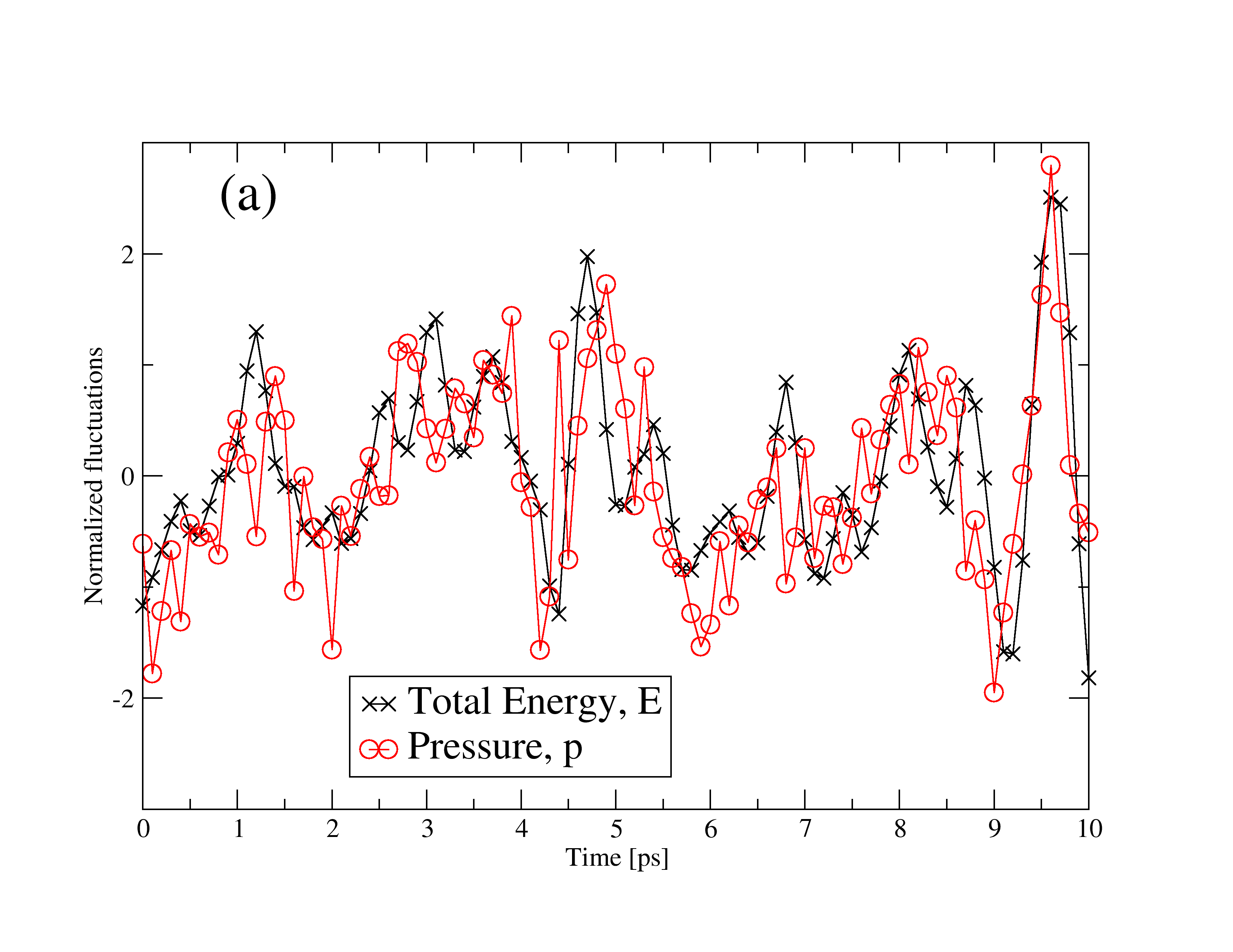
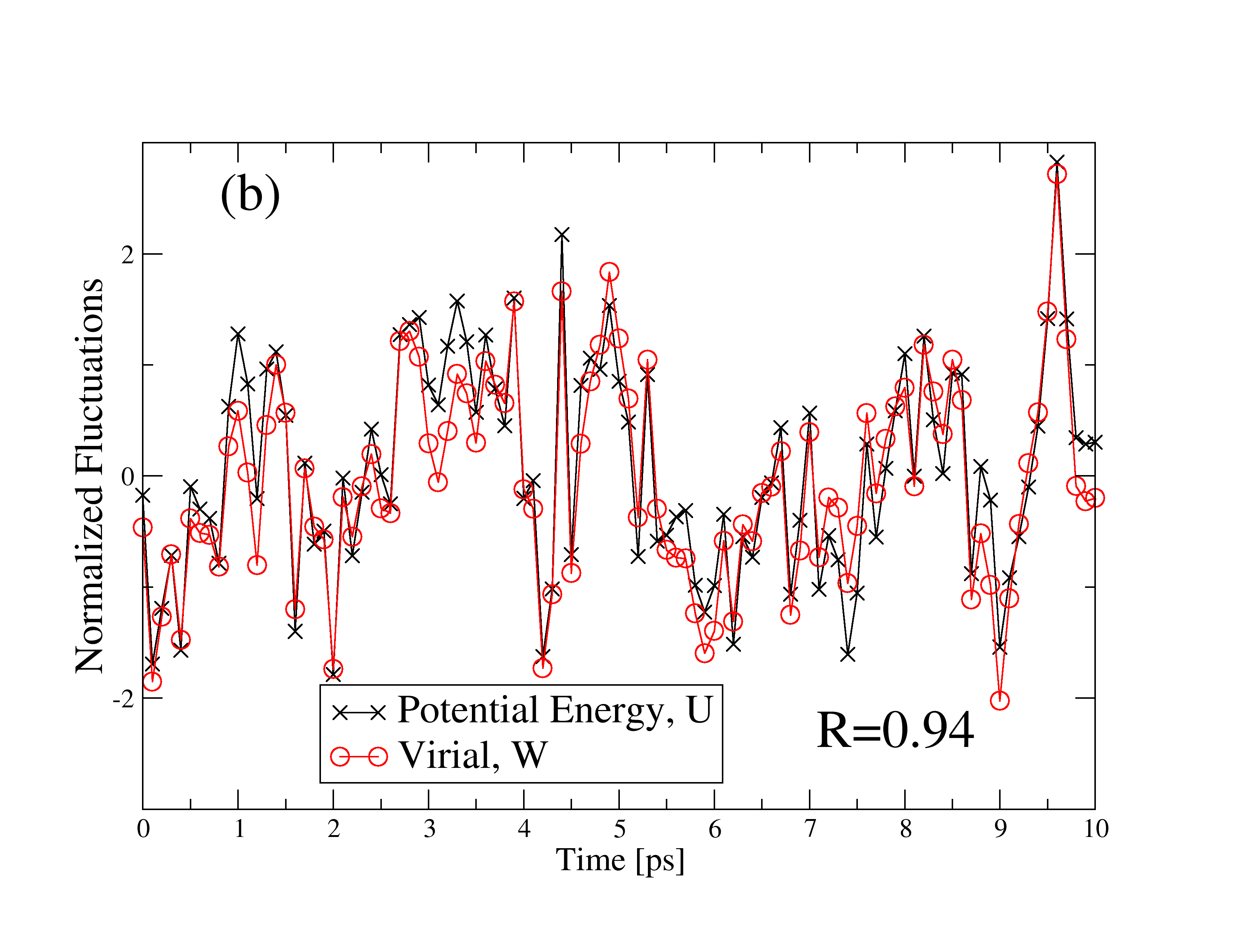
Figure 1: (Color online) Equilibrium fluctuations of (a) pressure $p$ and energy $E$ and (b) virial $W$ and potential energy $U$, in a single-component Lennard-Jones system simulated in the NVT ensemble at $\rho=34.6$ mol/l and $T=80$K (Argon units). The time-averaged pressure was close to zero (1.5 MPa). The correlation coefficient $R$ between $W$ and $U$ is 0.94, whereas the correlation coefficient is only 0.70 between $p$ and $E$. Correlation coefficients were calculated over the total simulation time (10 ns).

Physicists are familiar with the idea of thermal fluctuations in equilibrium. They also know how to extract useful information from them, using linear response theory.Landau and Lifshitz (1980); Hansen and McDonald (1986); Reichl (1998); Allen and Tildesley (1987) These methods started with Einstein’s observation that the specific heat in the canonical ensemble is determined by the magnitude of energy fluctuations. In any thermodynamic system some variables are fixed, and some fluctuate. The magnitude of the variances of the latter, and of the their mutual covariance, determine the thermodynamic “response” parameters.Landau and Lifshitz (1980) For example, in the canonical (NVT) ensemble, pressure $p$ and energy $E$ fluctuate; the magnitude of pressure fluctuations is related to the isothermal bulk modulus $K_{T}\equiv-V\left(\frac{\partial p}{\partial V}\right)_{T}$, that of the energy fluctuations to the specific heat at constant volume $c_{V}\equiv T\left(\frac{\partial S}{\partial T}\right)_{V}$, while the covariance $\langle\Delta p\Delta E\rangle$ is relatedAllen and Tildesley (1987) to the thermal pressure coefficient $\beta_{V}\equiv\left(\frac{\partial p}{\partial T}\right)_{V}$. If the latter is non-zero, it implies a degree of correlation between pressure and energy fluctuations. There is no obvious reason to suspect any particularly strong correlation, and to the best of our knowledge none has ever been reported. But in the course of investigating the physics of highly viscous liquids by computer simulation, we noted strong correlations between pressure and energy equilibrium fluctuations in several model liquids, also in the high temperature, low-viscosity state. These included the most studied of all computer liquids, the Lennard-Jones system. Surprisingly, these strong correlations survive crystallization, and they are also present in the glass phase. “Strong” here and henceforth means a correlation coefficient of order 0.9 or larger. In this paper we examine several model liquids and detail which systems exhibit strong correlations and which do not. In the companion paperBailey et al. (2008) (referred to as Paper II) we present a detailed analysis of the correlations for the single-component Lennard-Jones system, and discuss some consequences.

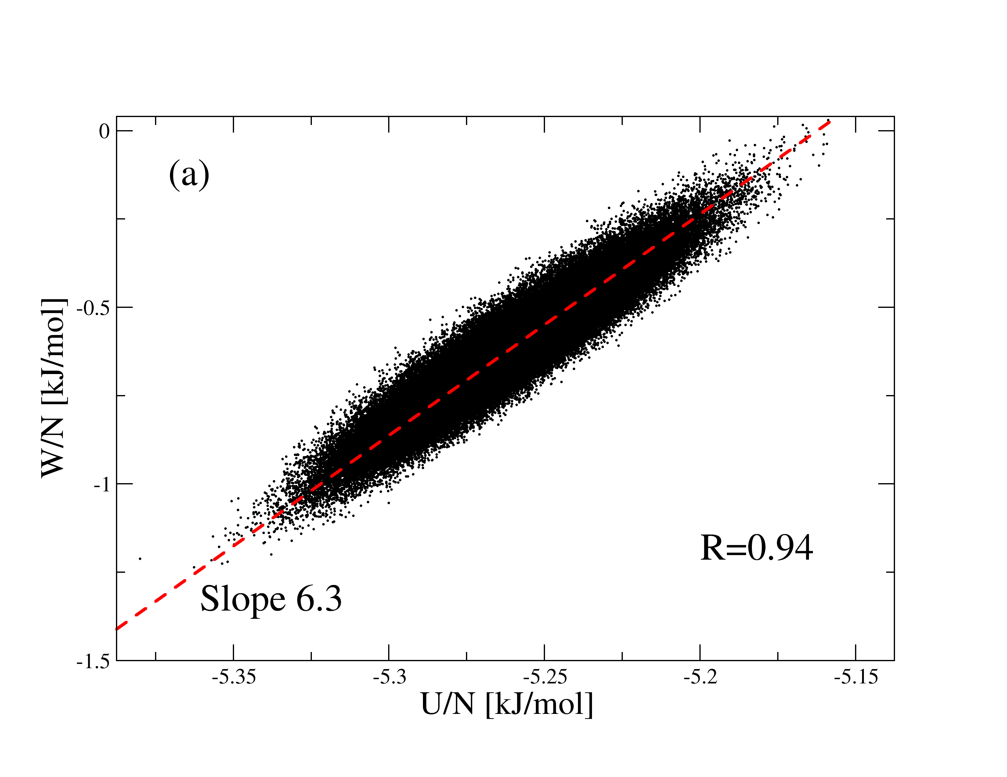
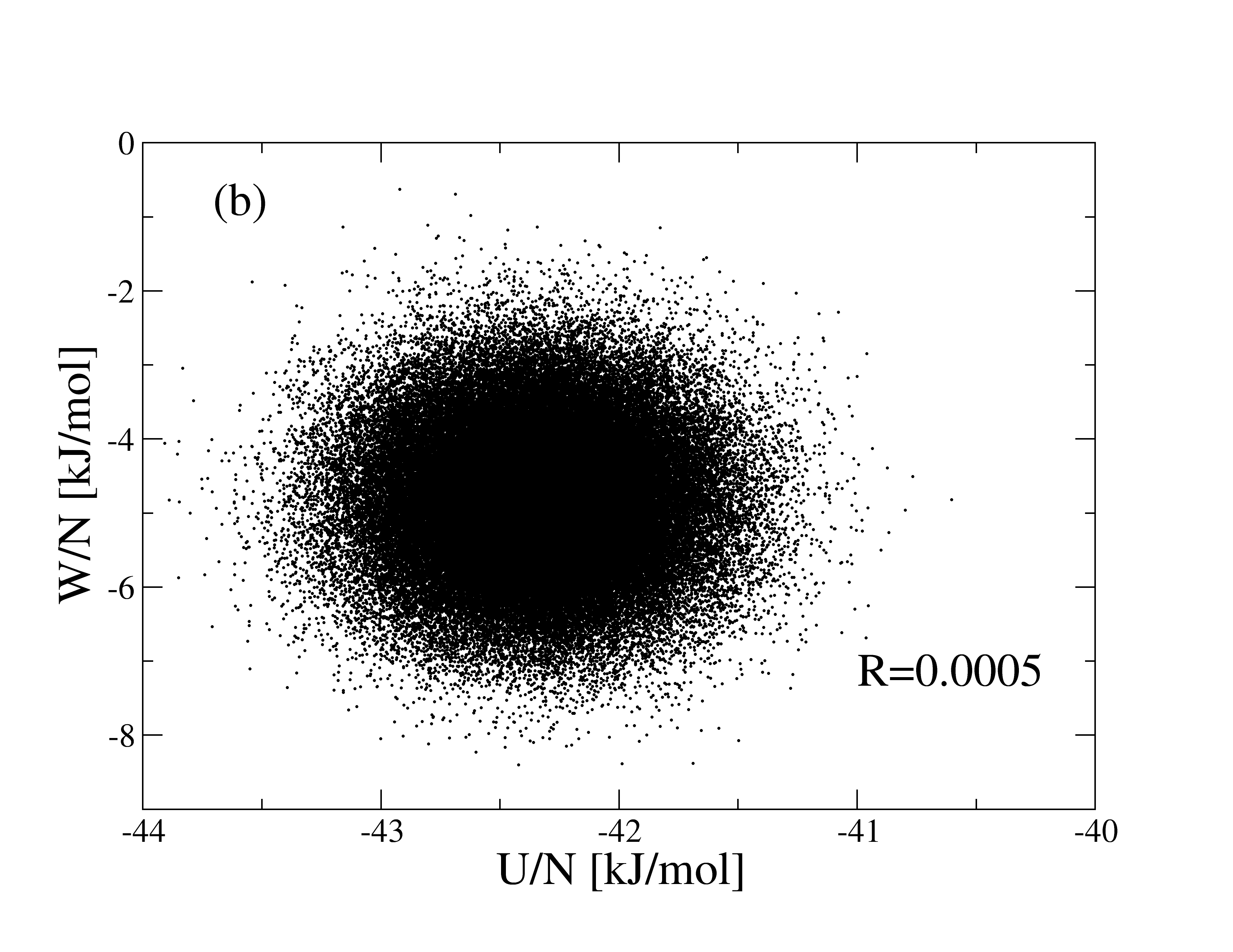
Figure 2: (Color online) (a) Scatter-plot of instantaneous virial $W$ and potential energy $U$ from the simulation of Fig. 1. The dashed line is a guide to the eye, with a slope determined by the ratio of standard deviations of $W$ and $U$ (Eq. (7)). (b) Example of a system with almost no correlation between $W$ and $U$: TIP5P water at T=12.5^∘C, density 1007.58 kg/m³ (NVT). This system has Coulomb, in addition to Lennard-Jones, interactions.

Specifically, the fluctuations which are in many cases strongly correlated are those of the configurational parts of pressure and energy (the parts in addition to the ideal gas terms). The (instantaneous) pressure $p$ and energy $E$ have contributions both from particle momenta and positions:

$$p =Nk_{B}T(\mathbf{p}_{1},\ldots,\mathbf{p}_{N})/V+W(\mathbf{r}_{1},\ldots,\mathbf{r}_{N})/V$$

$$E =K(\mathbf{p}_{1},\ldots,\mathbf{p}_{N})+U(\mathbf{r}_{1},\ldots,\mathbf{r}_{N}),$$ (1)

where $K$ and $U$ and the kinetic and potential energies, respectively. Here $T(\mathbf{p}_{1},\ldots,\mathbf{p}_{N})$ is the “kinetic temperature”,Allen and Tildesley (1987) proportional to the kinetic energy per particle. The configurational contribution to pressure is the virial $W$, which is definedAllen and Tildesley (1987) by

$$W=-\frac{1}{3}\sum_{i}\mathbf{r}_{i}\cdot\mathbf{\nabla}_{\mathbf{r}_{i}}U$$ (2)

where $\mathbf{r}_{i}$ is the position of the $i$th particle. Note that $W$ has dimension energy. For a pair interaction we have

$$U_{\textrm{pair}}=\sum_{i<j}v(r_{ij})$$ (3)

where $r_{ij}$ is the distance between particles $i$ and $j$ and $v(r)$ is the pair potential. The expression for the virial (Eq. (2)) becomesAllen and Tildesley (1987)

$$W_{\textrm{pair}}=-\frac{1}{3}\sum_{i<j}r_{ij}v^{\prime}(r_{ij})=-\frac{1}{3}\sum_{i<j}w(r_{ij})$$ (4)

where for convenience we define

$$w(r)\equiv rv^{\prime}(r).$$ (5)

Fig. 1 (a) shows normalized instantaneous values of $p$ and $E$, shifted and scaled to have zero mean and unit variance, as a function of time for the standard single-component Lennard-Jones (SCLJ) liquid, while Fig. 1 (b) shows the corresponding fluctuations of $W$ and $U$. We quantify the degree of correlation by the standard correlation coefficient $R$, defined by

$$R=\frac{\langle\Delta W\Delta U\rangle}{\sqrt{\langle(\Delta W)^{2}\rangle}\sqrt{\langle(\Delta U)^{2}\rangle}}.$$ (6)

Here angle brackets $\langle\rangle$ denote thermal averages while $\Delta$ denotes deviation from the average value of the given quantity. The correlation coefficient is ensemble-dependent, but our main focus—the $R\rightarrow 1$ limit–is not. Most of the simulations reported below were carried out in the NVT ensemble. Another important characteristic quantity is the “slope” $\gamma$, which we define as the ratio of standard deviations:

$$\gamma\equiv\frac{\sqrt{(\Delta W)^{2}}}{\sqrt{(\Delta U)^{2}}}.$$ (7)

Considering the “total” quantities, $p$ and $E$, (Fig. 1(a)) there is some correlation; the correlation coefficient $0.70$. For the configurational parts, $W$ and $U$, on the other hand (Fig. 1(b)), the degree of correlation is much higher, $R=0.94$ in this case. Another way to exhibit the correlation is a scatter-plot of $W$ against $U$, as shown in Fig. 2(a).

Is this correlation surprising? Actually, there are some interatomic potentials for which there is a 100% correlation between virial and potential energy. If we have a pair potential of the form $v(r)\propto r^{-n}$, an inverse power-law, then $w(r)=-nv(r)$ and $W_{\textrm{pair}}=(n/3)U_{\textrm{pair}}$ holds exactly. In this case the correlation is 100% and $\gamma=n/3$.

Conversely, suppose a system is known to be governed by a pair potential, and that there is 100% correlation between $W$ and $U$. We can write both $U$ and $W$ at any given time $t$ as integrals over the instantaneous radial distribution function definedAllen and Tildesley (1987) as

$$g(r,t)\equiv\frac{2}{N\rho}\sum_{i<j}\delta(r-r_{ij}(t))/(4\pi r^{2})$$ (8)

from which

$$U(t)=\frac{N}{2}\rho\int_{0}^{\infty}\!dr\,4\pi r^{2}g(r,t)v(r)$$ (9)

and

$$W(t)=-\frac{N}{6}\rho\int_{0}^{\infty}\!dr\,4\pi r^{2}g(r,t)w(r).$$ (10)

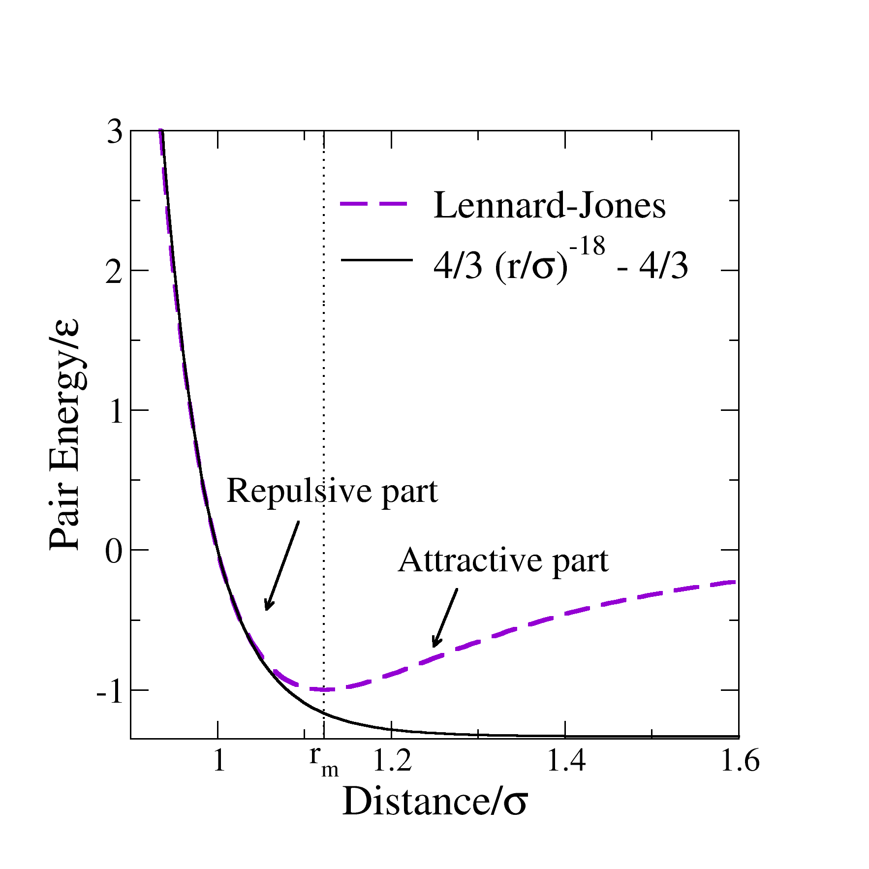
Figure 3: (Color online) Illustration of the “effective inverse power-law” chosen in this case to match the Lennard-Jones potential and its first two derivatives at the point $r=\sigma$. The vertical line marks the division into the repulsive and attractive parts of the Lennard-Jones potential.

Here the factor of $\frac{1}{2}$ is to avoid double-counting, and $\rho=N/V$ is the number density. 100% correlation means that $W(t)=\gamma U(t)$ holds for arbitrary $g(r,t)$ (a possible additive constant could be absorbed into the definition of $U$). In particular we could consider $g(r,t)=\delta(r-r_{0})$. Substituting this into the above expressions, the integrals go away and we find $w(r_{0})=-3\gamma v(r_{0})$. Since $r_{0}$ was arbitrary, $v^{\prime}(r)=-3\gamma v(r)/r$, which has the solution $v(r)\propto r^{-3\gamma}$. This connection between an inverse power-law potential and perfect correlations suggests that strong correlations can be attributed to an effective inverse power-law potential, with exponent given by three times the observed value of $\gamma$. This will be detailed in Paper II, which shows that while this explanation is basically correct, matters are somewhat more complicated than this. For instance, the fixed volume condition, under which the strong correlations are actually observed, imposes certain constraints on $g(r,t)$.

The celebrated Lennard-Jones potential is givenLennard-Jones (1931) by

$$v_{LJ}(r)=4\epsilon\left[\left(\frac{\sigma}{r}\right)^{12}-\left(\frac{\sigma}{r}\right)^{6}\right].$$ (11)

One might think that in the case of the Lennard-Jones potential the fluctuations are dominated by the repulsive $r^{-12}$ term, but this naïve guess leads to a slope of four, rather than the 6.3 seen in Fig. 2 (a). Nevertheless the observed correlation, and the above mentioned association with inverse power-law potentials, suggest that an effective inverse power-law description (involving short distances), with a more careful identification of the exponent, may apply. In fact, the presence of the second, attractive, term, increases the effective steepness of the repulsive part, thus increasing the slope of the correlation, or equivalently the effective inverse power-law exponent (Fig. 3). Note the distinction between repulsive term and repulsive part of the potential: the latter is the region where $v(r)$ has negative slope, thus the region $r<r_{m}$ ($r_{m}$ being the distance where the pair potential has its minimum, $2^{1/6}\sigma$ for $v_{LJ}$). This region involves both the repulsive and attractive terms (see Fig. 3, which also illustrates the approximation of the repulsive part by a power law with exponent 18). The same division was made by Weeks, Chandler, and Andersen (WCA) in their noted paper of 1971,Weeks et al. (1971) in which they showed that the the thermodynamic and structural properties of the Lennard-Jones fluid were dominated by the repulsive part at high temperatures for all densities, and also at low temperatures for high densities. Ben-Amotz and StellBen-Amotz and Stell (2003) noted that the repulsive core of the Lennard-Jones potential may be approximated by an inverse power-law with $n\sim$18–20. The approximation by an inverse power-law may be directly checked by computing the potential and virial with an inverse power-law potential for configurations drawn from actual simulations using the Lennard-Jones potential. The agreement (apart from additive constants) is good, see Paper II.

Consider now a system with different types of pair interactions, for example a binary Lennard-Jones system with AA, BB, and AB interactions, or a hydrogen-bonding system modelled via both Lennard-Jones and Coulomb interactions. We can write arbitrary deviations of $U$ and $W$ from their mean values, denoted $\Delta U$ and $\Delta W$, as a sum over types (indexed by $t$; sums over pairs of a given type are implicitly understood):

$$\Delta U=\sum_{t}\Delta U_{t};\ \Delta W=\sum_{t}\Delta W_{t}.$$ (12)

Now, supposing there is near-perfect correlation for the individual terms with corresponding slopes $\gamma_{t}$, we can rewrite $\Delta W$ as

$$\Delta W=\sum_{t}\gamma_{t}\Delta U_{t}.$$ (13)

If the $\gamma_{t}$ are all more or less equal to a single value $\gamma$, then this can be factored out and we get $\Delta W\simeq\gamma\Delta U$. Thus the existence of different Lennard-Jones interactions in the same system does not destroy the correlation, since they have $\gamma_{t}\sim 6$. On the other hand the slope for Coulomb interaction, which as an inverse power-law has perfect $W,U$ correlations, is $1/3$, so we cannot expect overall strong correlation in this case (Fig. 2 (b)). Indeed such reasoning also accounts for the reduction of correlation when the total pressure and energy are considered: $\Delta E=\Delta U+\Delta K$, while (for a large atomic system) $V\Delta p=\gamma\Delta U+(2/3)\Delta K$. The fact that $\gamma$ is (for the Lennard-Jones potential) quite different from 2/3 implies that the $p,E$ correlation is significantly weaker that of $W,U$ (Fig. 1). Even in cases of unequal slopes, however, there can be circumstances under which one kind of term, and therefore one slope, dominates the fluctuations. In this case strong correlations will be observed. Examples include the high-temperature limits of hydrogen-bonded liquids (section III.4) and the time-averaged (total) energy and pressure in viscous liquids (Paper II).

Some of the results detailed below were published previously in Letter form;Pedersen et al. (2008a) the aim of the present contribution is to make a comprehensive report covering more systems, while Paper II contains a detailed analysis and discusses applications. In the following section, we describe the systems simulated. In section III we present the results for all the systems investigated, in particular the degree of correlation (correlation coefficient $R$) and the slope. Section IV gives a summary.

II Simulated systems

A range of simulation methods, thermodynamic ensembles and computational codes were used. One reason for this was to eliminate the possibility that the strong correlations are an artifact of using a particular ensemble or code. In addition, no one code can simulate the full range of systems presented. Most of the data we present are from molecular dynamics (MD) simulations, although some are from Monte Carlo Landau and Binder (2005) (MC) and event-drivenZaccarelli et al. (2002) (ED) simulations. Most of the MD simulations (and of course all MC simulations), had fixed temperature (NVT), while some had fixed total energy (NVE). Three MD codes were used: Gromacs (GRO),Berendsen et al. (1995); Lindahl et al. (2001) Asap (ASAP), Asap and DigitalMaterial (DM). Bailey et al. (2006) Home-made (HM) codes were used for the MC and ED simulations.

We now list the thirteen systems studied, giving each a code-name for future reference. The systems include monatomic systems interacting with pair potentials, binary atomic systems interacting with pair potentials, molecular systems consisting of Lennard-Jones particles joined rigidly together in a fixed configuration (here the Lennard-Jones interaction models the van der Waals forces), molecular systems which have Coulomb as well as Lennard-Jones interactions, metallic systems with a many-body potential, and a binary system interacting with a discontinuous “square-well” potential. Included with each system is a list specifying which simulation method(s), which ensemble(s), and which code(s) were used (semi-colons separate the method(s) from the ensemble(s) and the ensemble(s) from the code(s)). Details of the potentials are given in Appendix A.

CU

Pure liquid Cu simulated using the many-body potential derived from effective medium theory (EMT); Jacobsen et al. (1987, 1996) (MD; NVE; ASAP)

DB

Asymmetric “dumb-bell” molecules,Pedersen et al. (2008b) consisting of two unlike Lennard-Jones spheres connected by a rigid bond; (MD; NVT; GRO)

DZ

The potential introduced by DzugutovDzugutov (1992) as a candidate for a monatomic glass-forming system. Its distinguishing feature is a peak in $v(r)$ around 1.5$\sigma$, after which it decays exponentially to zero at a finite value of $r$; (MD; NVT, NVE; DM)

EXP

A system interacting with a pair potential with exponential repulsion and a van der Waals attraction; (MC; NVT; HM)

KABLJ

The Kob-Andersen binary Lennard-Jones liquid;Kob and Andersen (1994) (MD; NVT, NVE; GRO, DM)

METH

The GromosScott et al. (1999) 3-site model for methanol; (MD; NVT; GRO)

MGCU

A model of the metallic alloy Mg₈₅Cu₁₅ using an EMT-based potential; Bailey et al. (2004) (MD; NVE; ASAP)

OTP

A three-site model of the fragile glass-former Ortho-terphenyl (OTP);Lewis and Wahnström (1994)(MD; NVT; GRO)

SCLJ

The standard single-component Lennard-Jones system with the interaction given in Eq. (11); (MD, MC; NVT, NVE; GRO, DM)

SPC/E

The SPC/E model of water;Berendsen et al. (1987) (MD; NVT; GRO)

SQW

A binary model with a pair interaction consisting of an infinitely hard core and an attractive square well; Zaccarelli et al. (2002, 2004)(ED; NVE; HM)

TIP5P

A five-site model for liquid water which reproduces the density anomaly.Mahoney and Jorgensen (2000) (MD; NVT; GRO)

TOL

A 7-site united-atom model of toluene; (MD; NVT; GRO)

The number of particles (atoms or molecules) was in the range 500–2000. Particular simulation parameters ($N$, $\rho$, $T$, duration of simulation) are given when appropriate in the results section.

III Results

III.1 The standard single-component Lennard-Jones system

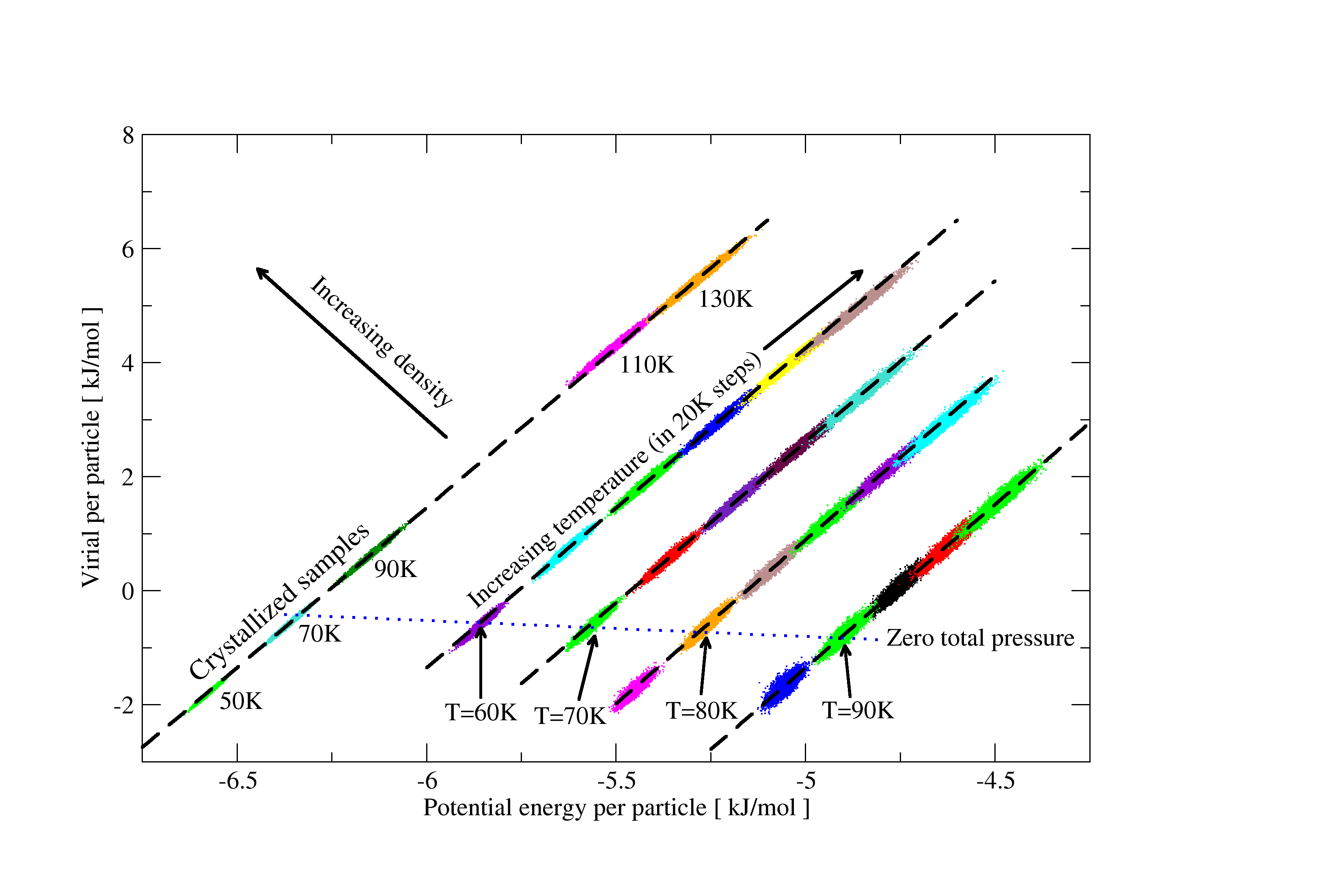
Figure 4: (Color online) Scatter plots of the configurational parts of pressure and energy – virial versus potential energy – for several state points of the single-component Lennard-Jones liquid (NVT). Each oval represents simulations at one particular temperature and density where each data point marks instantaneous values of virial and potential energy. The dashed lines mark constant density paths with the highest density to the upper left (densities: 39.8 mol/l, 37.4 mol/l, 36.0 mol/l, 34.6 mol/l, 32.6 mol/l). State points on the dotted line have zero average pressure. The plot includes three crystallized samples (lower left corner), discussed at the end of section III.1 and, in more detail, in Paper II [reproduced from Ref. Pedersen et al., 2008a].

Table 1: Correlation coefficients $R$ and effective slopes $\gamma$ for the single-component Lennard-Jones system (SCLJ) for the state points in Fig. 4. $p$ is the thermally averaged pressure. The last five states were chosen to approximately follow the isobar $p=0$.

$\rho$ (mol/l)	$T$(K)	p(MPa)	phase	$R$	$\gamma$
42.2	12	2.6	glass	0.905	6.02
39.8	50	-55.5	crystal	0.987	5.85
39.8	70	-0.5	crystal	0.989	5.73
39.8	90	54.4	crystal	0.990	5.66
39.8	110	206.2	liquid	0.986	5.47
39.8	150	309.5	liquid	0.988	5.34
37.4	60	-3.7	liquid	0.965	6.08
37.4	100	102.2	liquid	0.976	5.74
37.4	140	192.7	liquid	0.981	5.55
37.4	160	234.3	liquid	0.983	5.48
36.0	70	-0.7	liquid	0.954	6.17
36.0	110	90.3	liquid	0.969	5.82
36.0	150	169.5	liquid	0.977	5.63
36.0	190	241.4	liquid	0.981	5.49
36.0	210	275.2	liquid	0.982	5.44
34.6	60	-42.5	liquid	0.900	6.53
34.6	100	41.7	liquid	0.953	6.08
34.6	140	114.5	liquid	0.967	5.80
34.6	200	211.0	liquid	0.977	5.57
32.6	70	-35.6	liquid	0.825	6.66
32.6	90	-0.8	liquid	0.905	6.42
32.6	110	31.8	liquid	0.929	6.22
32.6	150	91.7	liquid	0.954	5.95
32.6	210	172.7	liquid	0.968	5.68
37.4	60	-3.7	liquid	0.965	6.08
36.0	70	-0.7	liquid	0.954	6.17
34.6	80	1.5	liquid	0.939	6.27
32.6	90	0.0	liquid	0.905	6.42
42.2	12	2.6	glass	0.905	6.02

SCLJ is the system we have most completely investigated. $W,U$-plots are shown for a range of thermodynamic state points in Fig. 4. Here the ensemble was NVT with N=864, and each simulation consisted of a 10 ns run taken after 10ns of equilibration; for all SCLJ results so-called “Argon” units are used ($\sigma=0.34$ nm, $\epsilon=0.997$ kJ/mol). Each elongated oval in Fig. 4 is a collection of $W,U$ pairs for a given state point. Varying temperature at fixed density moves the oval parallel to itself, following an almost straight line as indicated by the dashed lines. Different densities correspond to different lines, with almost the same slope. In a system with a pure inverse power-law interaction, the correlation would be exact, and moreover the data for all densities would fall on the same straight line (see the discussion immediately after Eq. (5)). Our data, on the other hand, show a distinct dependence on volume, but for a given volume, because of the strong correlation, the variation in $W$ is almost completely determined by that of $U$.

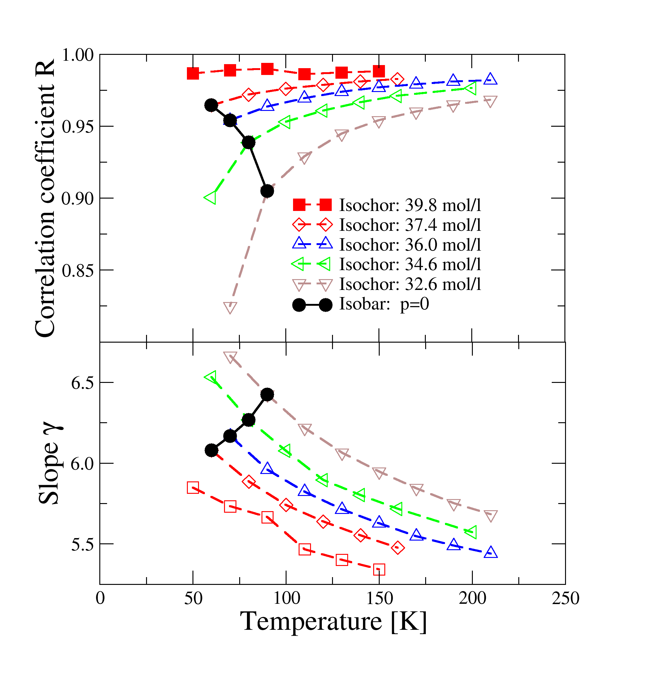
Figure 5: (Color online) Upper plot, correlation coefficient $R$ for the SCLJ system as a function of temperature for several densities (NVT). This figure makes clear the different effects of density and temperature on $R$. Lower plot, effective slope $\gamma$ as a function of $T$. Simulations at temperatures higher than those shown here indicate that the slope slowly approaches the value four as $T$ increases. This is to be expected because as collisions become harder, involving shorter distances, the effective inverse power-law exponent approaches the 12 from the repulsive term of the Lennard-Jones potential.

Values of correlation coefficient $R$ for the state points of Fig. 4 are listed in Table 1, along with the slope $\gamma$. In Fig. 5 we show the temperature dependence of both $R$ and $\gamma$ for different densities. Lines have been drawn to indicate isochores and one isobar ($p=0$). Note that when we talk of an isobar here, we mean a set of NVT ensembles with $V,T$ chosen so that the thermal average of $p$ takes on a given value, rather than fixed-pressure ensembles. This figure makes it clear that for fixed density, $R$ increases as $T$ increases, while it also increases with density for fixed temperature; the slope slowly decreases in these circumstances. In fact it eventually reaches four, the value expected for a pure $r^{-12}$ interaction (e.g., at $\rho=34.6$ mol/l, $T=1000$ K, $\gamma=4.61$, see Ref. Pedersen et al., 2008a). This is consistent with the idea that the repulsive part, characterized by an effective inverse power-law, dominates the fluctuations: increasing either temperature or density increases the frequency of short-distance encounters while reducing the typical distances of such encounters. On the other hand, along an isobar, these two effects work against each other, since as $T$ increases, the density decreases. The density effect “wins” in this case, which is equivalent to a statement about the temperature and volume derivative of $R$: Our simulations imply that

$$\left(\frac{\partial R}{\partial T}\right)_{p}=\left(\frac{\partial R}{\partial T}\right)_{V}+\left(\frac{\partial R}{\partial V}\right)_{T}\left(\frac{\partial V}{\partial T}\right)_{p}<0$$ (14)

which is equivalent to

$$\left(\frac{\partial R}{\partial T}\right)_{V}<-\left(\frac{\partial R}{\partial V}\right)_{T}V\alpha_{p}=\rho\left(\frac{\partial R}{\partial\rho}\right)_{T}\alpha_{p}$$ (15)

where $\alpha_{p}\equiv(\partial V/\partial T)_{p}/V$ is the thermal expansivity at constant pressure and $\rho$ is the particle density. This can be recast in terms of logarithmic derivatives (valid whenever $(\partial R/\partial\rho)_{T}>0$) as follows

$$\frac{\left(\frac{\partial R}{\partial\ln(T)}\right)_{V}}{\left(\frac{\partial R}{\partial\ln(\rho)}\right)_{T}}<T\alpha_{p}.$$ (16)

Thus what we observe in the simulations, namely that the correlation becomes stronger as temperature is reduced at fixed pressure, is a priori more to be expected when the thermal expansivity is large (since then the right hand side of Eq. (16) is large). This has particular relevance in the context of supercooled liquids, which we discuss in paper II, because these are usually studied by lowering temperature at fixed pressure. On the other hand if the expansivity becomes small, as for example, when a liquid passes through the glass transition, the inequality (16) is a priori less likely to be satisfied. We have in fact observed this in a simulation of OTP: upon cooling through the (computer) glass transition, the correlation became weaker with further lowering of temperature at constant pressure.

Remarkably, the correlation persists when the system has crystallized, as seen in the data for the highest density—the occurrence of the first-order phase transition can be inferred from the gap between the data for 90K and 110K, but the data fall on the same line above and below the transition. One would not expect the dynamical fluctuations of a crystal, which are usually assumed to be well-described by a harmonic approximation, to resemble those of the high-temperature liquid. In fact for a one-dimensional crystal of particles interacting with a harmonic potential $v(r)=\frac{1}{2}k(r-r_{m})^{2}$ it is easy to show (Paper II) that there is a negative correlation with slope equal to -2/3. To investigate whether the harmonic approximation ever becomes relevant for the correlations, we prepared a perfect FCC crystal of SCLJ particles at zero temperature and simulated it at increasing temperatures, from 0.02K to 90K in Argon units, along a constant density path. The results are shown in Fig. 6. Clearly the correlation is maintained right down to zero temperature. The harmonic approximation is therefore useless for dealing with the pressure fluctuations even as $T\rightarrow 0$, because the slope is far from -2/3. The reason for this is that the dominant contribution to the virial fluctuations comes from the third order term, as shown in Paper II.

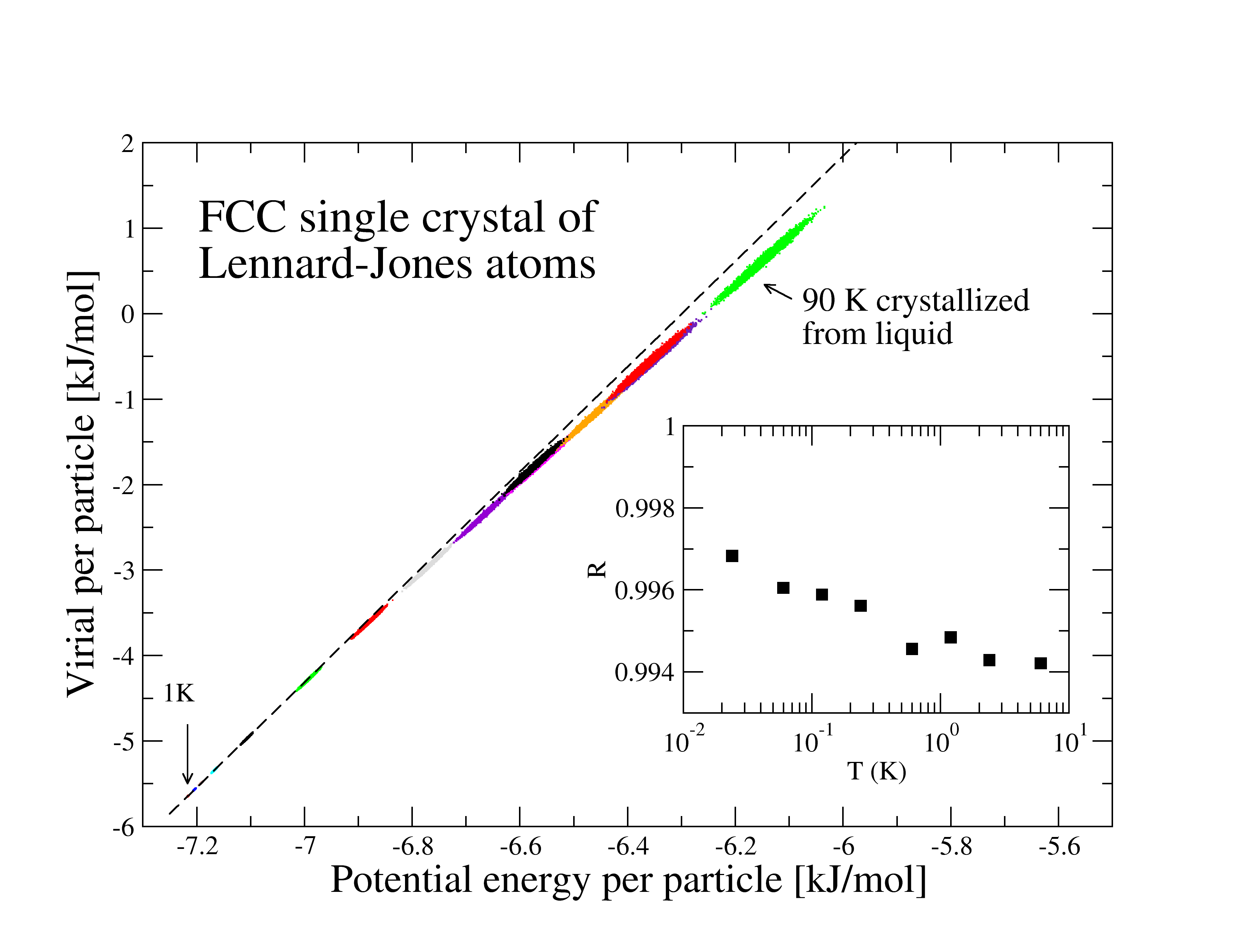
Figure 6: (Color online) Scatter-plot of the $W,U$ correlations for a perfect face-centered cubic (FCC) crystal of Lennard-Jones atoms at temperatures 1K, 2K, 3K, 5K, 10K, 20K, 30K, 40K, 50K, 60K, 70K and 80K, as well as for defective crystals (i.e., crystallized from the liquid) at temperatures 50K, 70K and 90K (NVT). The dashed line gives the best fit to the (barely visible) lowest-temperature data ($T=1$ K). The inset shows the temperature dependence of $R$ at very low temperatures. The crystalline case is examined in detail in Paper II, where we find that $R$ does not converge to unity at $T=0$, but rather to a value very close to unity.

III.2 A case with little correlation: the Dzugutov system

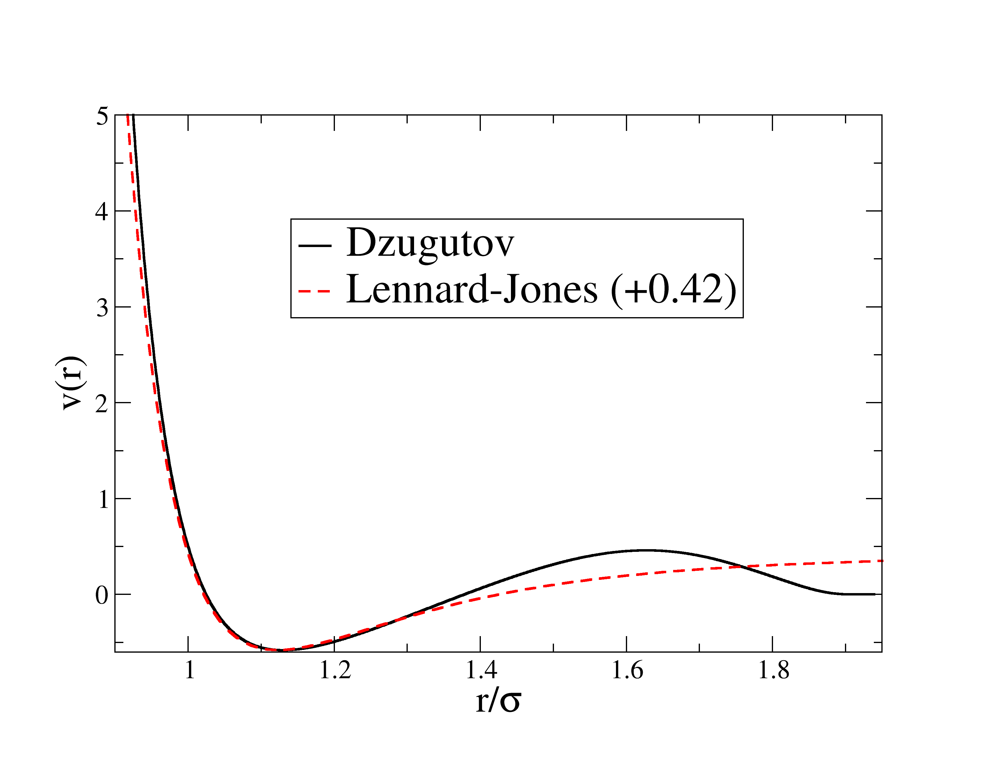
Figure 7: (Color online) A plot of the Dzugutov pair potential, with the Lennard-Jones potential (shifted by a constant) shown for comparison.

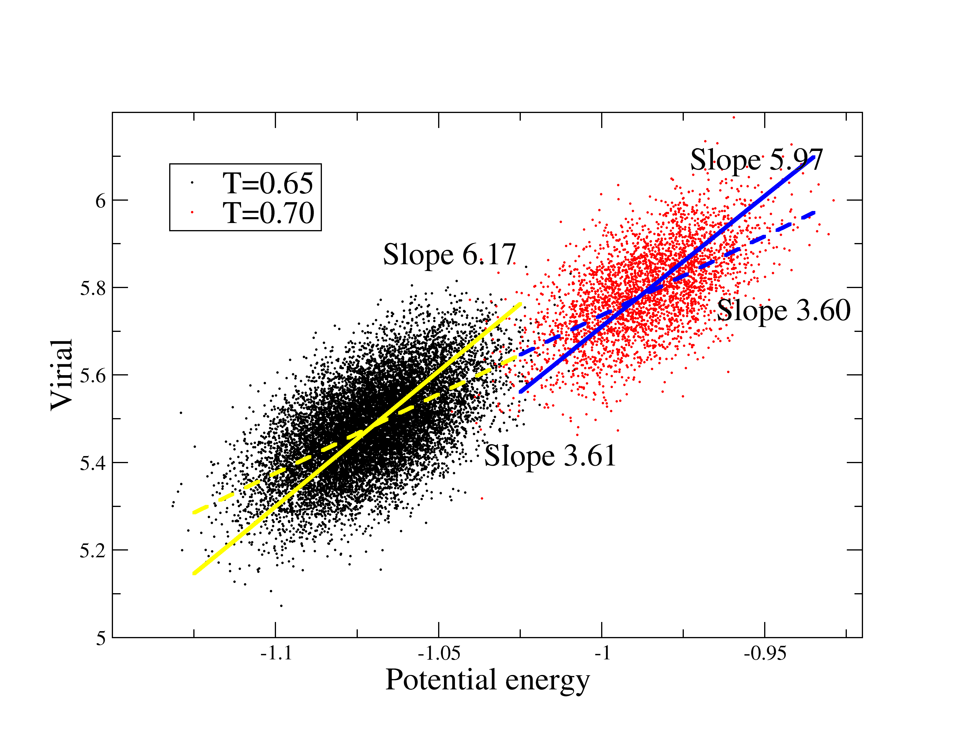
Figure 8: (Color online) Scatter-plot of $W,U$ correlations for the Dzugutov system at density 0.88 and temperatures 0.65 and 0.70 (NVE). The dashed lines indicate the best-fit line using linear regression. These are consistent with the temperature dependence of the mean values of $\langle W\rangle$ and $\langle U\rangle$, as they should be (see appendix B), but they clearly do not represent the direction of greatest variance. The full lines have slopes equal to the ratio of standard deviations of the two quantities (Eq. (7)). The correlation coefficient is 0.585 and 0.604 for $T=0.65$ and $T=0.70$, respectively.

Before presenting data for all the systems studied, it is useful to see what it means for the correlation not to hold. In this subsection we consider the Dzugutov system,Dzugutov (1992) whose potential contains a peak at the second-neighbor distance, (Fig. 7, see appendix A for details) whose presence might be expected to interfere with the effectiveness of an inverse power-law description. In the next subsection we show how in a specific model of water the lack of correlation can be explicitly seen to be the result of competing interactions. Fig. 8 shows $W,U$ plots for the Dzugutov system for two nearby temperatures at the same density. The ovals are much less elongated than was the case for SCLJ, indicating a significantly weaker correlation—the correlation coefficients here are 0.585 and 0.604, respectively. In paper II it is shown explicitly that the weak correlation is due to contributions arising from the second peak. Note that the major axes of the ovals are not aligned with the line joining the state points, given by the mean values of $W$ and $U$, here identifiable as the intersection of the dashed and straight lines. On the other hand, the lines of best fit from linear regression, indicated by the dashed lines in each case, do coincide with the line connecting state points. This holds generally, a fact which follows from statistical mechanics (appendix B). The interesting thing is rather that the major axes point in different directions, whereas in the SCLJ case they are also aligned with the state-point line. The linear-regression slope, being equal to $\langle\Delta U\Delta W\rangle/\langle(\Delta U)^{2}\rangle$, treats $W$ and $U$ in an asymmetric manner by involving $\langle(\Delta U)^{2}\rangle$, but not $\langle(\Delta W)^{2}\rangle$. This is because a particular choice of independent and dependent variables is made. If instead we plotted $U$ against $W$, we would expect the slope to be simply the inverse of the slope in the $W,U$ plot, but in fact the new slope is $\langle\Delta U\Delta W\rangle/\langle(\Delta W)^{2}\rangle$. This equals the inverse of the original slope only in the case of perfect correlation, where $\langle\Delta U\Delta W\rangle^{2}=\langle(\Delta W)^{2}\rangle\langle(\Delta U)^{2}\rangle$. For our purposes a more symmetric estimate of the slope is desired, one which agrees with the linear regression slope in the limit of perfect correlation. We use simply the ratio of standard deviations $\sqrt{\langle(\Delta W)^{2}\rangle}/\sqrt{\langle(\Delta U)^{2}\rangle}$ (Eq. (7)). This slope was used to plot the dashed line in Fig. 2(a) and the full lines in Fig. 8, where it clearly represents the orientation of the data better.

III.3 When competition between van der Waals and Coulomb interactions kills the correlation: TIP5P water

As we shall see in the next section, the systems which show little correlation include several which involve both van der Waals and Hydrogen bonding, modeled by Lennard-Jones and Coulomb interactions respectively. As noted already, the latter, being a pure inverse power-law ($n=1$), by itself exhibits perfect correlation with slope $\gamma=1/3$, while the Lennard-Jones part has near perfect correlation. But the significant difference in slopes means that no strong correlation is seen for the full interaction. To check explicitly that this is the reason the correlation is destroyed we have calculated the correlation coefficients for the Lennard-Jones and Coulomb parts separately in a model of water. Water is chosen because the density of Hydrogen bonds is quite high. Simulations were done with the TIP5P model of water Mahoney and Jorgensen (2000) which has the feature that the density maximum is reasonably well reproduced. This existence of the density maximum is in fact related to pressure and energy becoming uncorrelated, as we shall see.

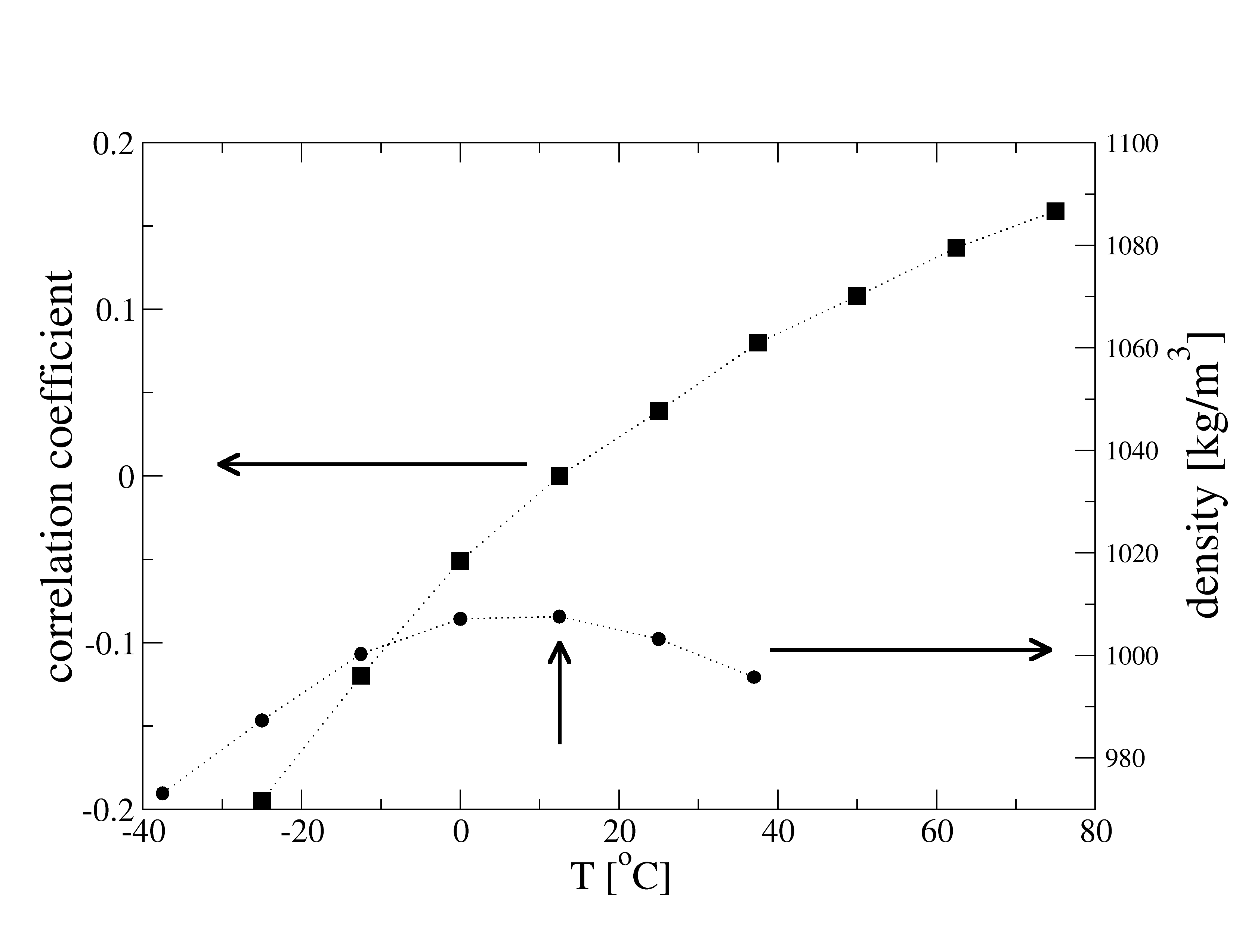
Figure 9: Plot of $R$ for TIP5P water in NVT simulations with densities chosen to give an average pressure of one atmosphere. Not only is the magnitude of $R$ low (less than 0.2) in the temperature range shown, but it changes sign around the density maximum. The vertical arrow indicates the state point used for Fig. 2 (b).

Figure 9 shows the correlation coefficients and slopes for a range of temperatures; the correlation is almost non-existent, passing through zero around where the density attains its maximum value. We have separately determined the correlation coefficient of the Lennard-Jones part of the interaction; it ranges from 0.9992 at -25 ^∘C to 0.9977 at 75 ^∘C, even larger than we have seen in the SCLJ system. The reason for this is that the (attractive) Coulomb interaction forces the centers of the Lennard-Jones interaction closer together than they would be otherwise, thus the relevant fluctuations are occurring higher up the repulsive part of the Lennard-Jones pair potential. Correspondingly the slope from this interaction ranges between 4.45 and 4.54, closer to the high-$T$, high density limit of 4 than was the case for the SCLJ system. This is confirmed by inspection of the oxygen-oxygen radial distribution function in Ref. Mahoney and Jorgensen, 2000 where it can be seen that the first peak lies entirely to the left of the $v_{LJ}=0$ distance $\sigma=0.312$ nm. Finally note that the near coincidence between the vanishing of the correlation coefficient and the density maximum, which is close to the experimental value of 4^∘C, is not accidental: The correlation coefficient is proportional to the configurational part of the thermal pressure coefficient $\beta_{V}$ (Paper II). The full $\beta_{V}$ vanishes exactly at the density maximum (4^∘C), but the absence of the kinetic term means that the correlation coefficient vanishes at a slightly higher temperature ($\sim 12^{\circ}$C).

III.4 Results for all systems

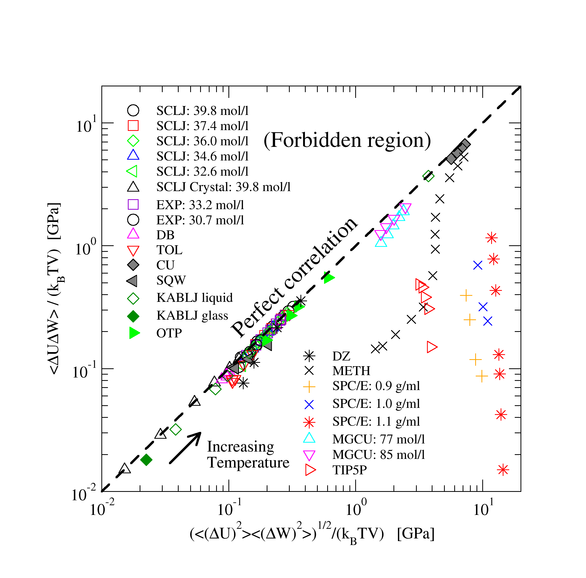
Figure 10: (Color online) $W,U$ correlations for all simulated liquids; $\left<\Delta W\Delta U\right>/(k_{B}TV)$ plotted versus $\left(\left<(\Delta W)^{2}\right>\left<(\Delta U)^{2}\right>\right)^{1/2}/(k_{B}TV)$. Both quantities correspond to a pressure, which is given in units of GPa; for model systems not specifically corresponding to real systems, such as SCLJ, KABLJ, SQW, Argon units were used to set the energy and length scales. If the correlation is perfect ($R=1$) the data fall on the diagonal marked by a dashed line. For the TIP5P model of water only temperatures with $R>0$ are included; volumes were chosen to give a pressure close to zero.

In Fig. 10 we summarize the results for the various systems. Here we plot the numerator of Eq. (6) against the denominator, including factors of $1/(k_{B}TV)$ in both cases to make an intensive quantity with units of pressure. Since $R$ cannot be greater than unity, no points can appear above the diagonal. Being exactly on the diagonal indicates perfect correlation ($R=1$), while being significantly below it indicates poor correlation. Different types of symbols indicate different systems, as well as different densities for the same system, while symbols of the same type correspond to different temperatures.

Table 2: Correlation coefficients and effective slopes at selected state points for all investigated systems besides SCLJ. Argon units were used for DZ, EXP, KABLJ and SQW by choosing the length parameter (of the larger particle when there were two types) to be 0.34 nm and the energy parameter to be 0.997 kJ/mol. The phase is indicated as liquid or glass. SQW data involves time averaging over periods 3.0, 3.0, 8.0 and 9.0, respectively, for the four listed state points. A minus sign has been included with the slope when $R<0$; note that the $\gamma$ values only really make sense as slopes when $|R|$ is close to unity. The ensemble was NVT except for CU, DZ, MGCU, and SQW, where it was NVE.

system	$\rho$(mol/L)	$T$(K)	phase	$R$	$\gamma$
CU	125.8	1500	liquid	0.907	4.55
CU	125.8	2340	liquid	0.926	4.15
DB	11.0	130	liquid	0.964	6.77
DB	9.7	300	liquid	0.944	7.45
DZ	37.2	78	liquid	0.585	3.61
EXP	30.7	96	liquid	0.908	5.98
EXP	33.2	96	liquid	0.949	5.56
KABLJ	50.7	30	glass	0.858	6.93
KABLJ	50.7	70	liquid	0.946	5.75
KABLJ	50.7	240	liquid	0.995	5.10
METH	31.5	150	liquid	0.318	22.53
METH	31.5	600	liquid	0.541	6.88
METH	31.5	2000	liquid	0.861	5.51
MGCU	85.0	640	liquid	0.797	4.74
MGCU	75.6	465	liquid	0.622	6.73
OTP	4.65	300	liquid	0.913	8.33
OTP	4.08	500	liquid	0.884	8.78
OTP	3.95	500	liquid	0.910	7.70
SPC/E	50.0	200	liquid	0.016	208.2
SPC/E	55.5	300	liquid	0.065	48.6
SQW	60.8	48	liquid	-0.763	-50.28
SQW	60.8	79	liquid	-0.833	-49.11
SQW	60.8	120	liquid	-0.938	-52.02
SQW	59.3	120	liquid	-0.815	-30.07
TIP5P	55.92	273	liquid	-0.051	-2.47
TIP5P	55.94	285.5	liquid	0.000	2.51
TOL	10.5	75	glass	0.877	7.59
TOL	10.5	300	liquid	0.961	8.27

All of the simple liquids, SCLJ, KABLJ, EXP, DB, TOL, show strong correlations, while METH, SPC/E, and TIP5P show little correlation. Values of $R$ and $\gamma$ at selected state points for all systems are listed in Table 2. What determines the degree of correlation? The Dzugutov and TIP5P cases have already been discussed. The poor correlation for METH and SPC/E is (presumably) because these models, like TIP5P, involve both Lennard-Jones and Coulomb interactions. In systems with multiple Lennard-Jones species, but without any Coulomb interaction, there is overall a strong correlation because the slope is almost independent of the parameters for a given kind of pair.

As the temperature is increased, the data for the most poorly correlated systems, which are all hydrogen-bonding organic molecules, slowly approach the perfect-correlation line. This is consistent with the idea that this correlation is observed when fluctuations of both $W$ and $U$ are dominated by close encounters of pairs of neighboring atoms; at higher temperature there are increasingly many such encounters, which therefore come to increasingly dominate the fluctuations. Also because the Lennard-Jones potential rises much more steeply than the Coulomb potential, the latter becomes less important as short distances dominate more. Although not obvious in the plot, we find that increasing the density at fixed temperature generally increases the degree of correlation, as found in the SCLJ case; this is also consistent with the increasing relevance of close encounters or collisions.

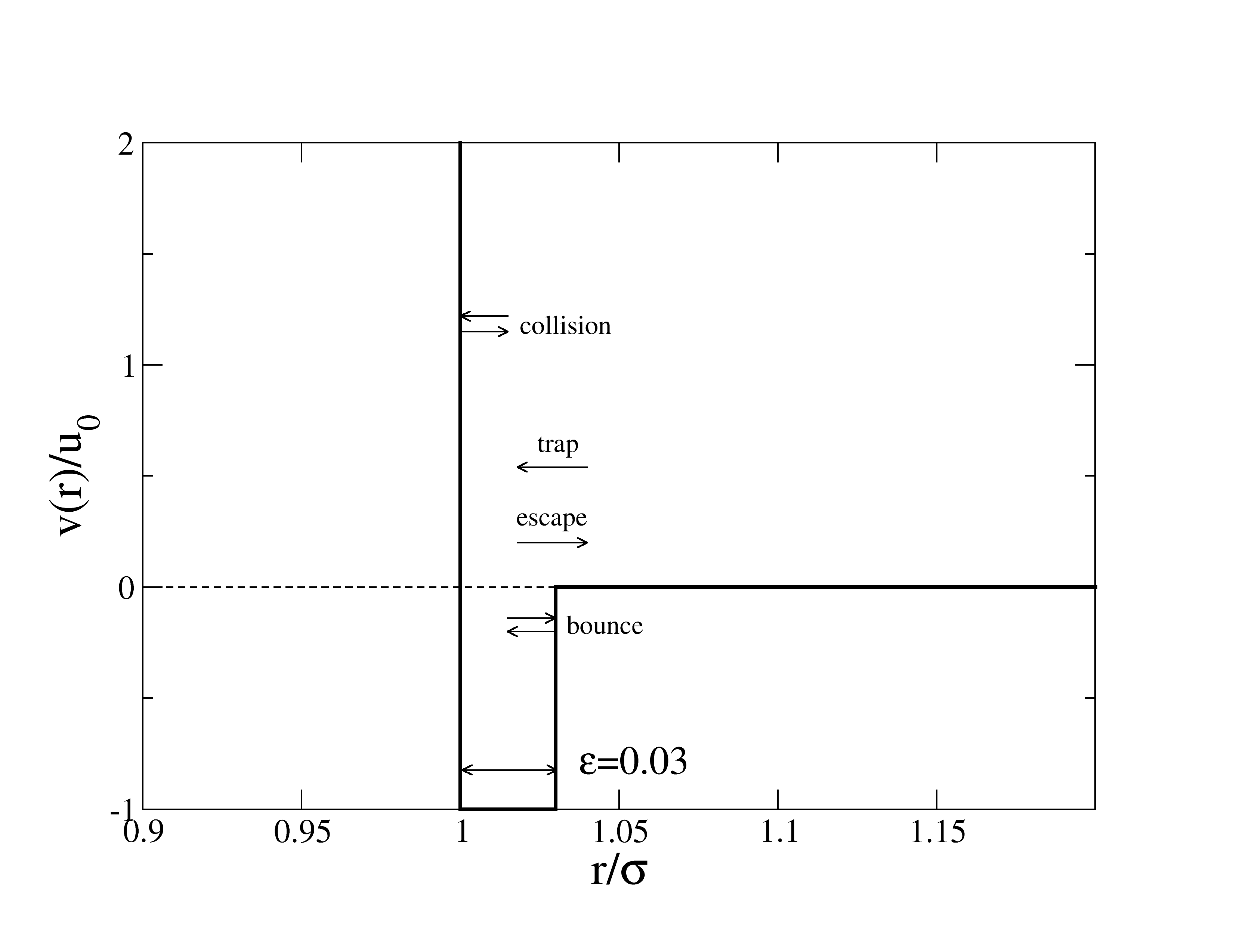
Figure 11: Illustration of the square-well potential, indicating the four microscopic processes which contribute to the virial.

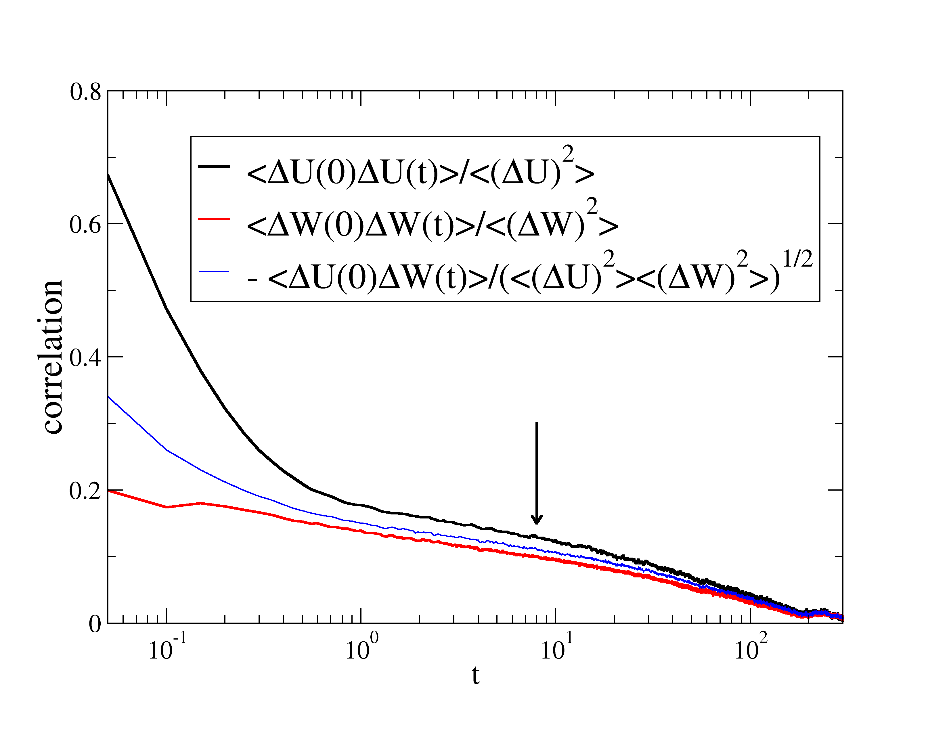
Figure 12: (Color online) Energy-energy, virial-virial, and energy-virial correlation functions for SQW at packing fraction $\phi=0.595$ and temperature $T=1.0$ (normalized to unity at $t=0$). The cross correlation has been multiplied by -1. The arrow marks the time $t=8$, roughly 1/10 of the relaxation time (determined from the long-time part of the energy-virial cross-correlation function). This time was used for averaging.

A system quite different from the others presented so far is the binary square-well system, SQW, with a discontinuous potential combining hard-core repulsion and a narrow attractive well (Fig. 11; see appendix A for details). Such a potential models attractive colloidal systems,Zaccarelli et al. (2002) one of whose interesting features, predicted from simulations and theory, is the existence of two different glass phases, termed the “repulsive” and “attractive” glasses. Sciortino (2002) The discontinuous potential not only makes the simulations substantially different from a technical point of view, but there are also conceptual differences—in particular, the instantaneous virial is a sum of delta-functions in time. The dynamical algorithm employed in the simulations is “event-driven”, where events involve a change in the relative velocity of a pair of particles due to hitting the hard-core inner wall of the potential or crossing the potential-step. The algorithm must detect the next event, advance time by the appropriate amount, and adjust the velocities of all particles appropriately. There are four kinds of events (illustrated in Fig. 11): (1) “collisions”, involving the inner repulsive core; (2) “bounces”, involving bouncing off the outer (attractive) wall of the potential; (3) “trapping”, involving the separation going below the range of the outer wall and (4) “escapes”, involving the separation increasing beyond the outer wall. To obtain meaningful values of the virial a certain amount of time-averaging must be done—we can no longer consider truly instantaneous quantities. As shown in appendix C the time-averaged virial may be written as the following sum over all events which take place in the averaging interval $t_{\textrm{av}}$:

$$\bar{W}=\frac{1}{3t_{\textrm{av}}}\sum_{\textrm{events}\,e}m_{r,e}\mathbf{r}_{e}\cdot\Delta\mathbf{v}_{e}$$ (17)

Here $\mathbf{r}_{e}$ and $\mathbf{v}_{e}$ refer to the relative position and velocity for the pair of particles participating in event $e$, while $\Delta$ indicates the change taking place in that event. Positive contributions to $\bar{W}$ come from collisions; the three other event types involve the outer wall, which, as is easy to see, always gives a negative contribution. The default $t_{\textrm{av}}$ in the simulation was 0.05. Strong correlations emerge only at longer averaging times, however. An appropriate $t_{\textrm{av}}$ may be chosen by considering the correlation functions (auto- and cross-) for virial and potential energy, plotted in Fig. 12, where the “instantaneous” values $E(t)$ and $W(t)$ correspond to averaging over 0.05 time units. We choose $t_{\textrm{av}}\simeq\tau_{\alpha}/10$, where $\tau_{\alpha}$ is the relaxation time determined from the cross-correlation function $\langle\Delta U(0)\Delta W(t)\rangle$. Data for a few state points are shown in Table 2. Remarkably, this system, so different from the continuous potential systems, also exhibits strong $W,U$-correlations, with $R=0.94$ in the case $T=1.0,\phi=0.595$ (something already hinted at in Fig. 12 in the fact that the curves coincide). There is a notable difference, however, compared to continuous systems: The correlation is negative.

The reason for the negative correlation is that at high density, most of the contributions to the virial are from collisions: a particle will collide with neighbor 1, recoil and then collide with neighbor 2 before there is a chance to make a bounce event involving neighbor 1. The number of collisions that occur in a given time interval is proportional to the number of bound pairs which is exactly anti-correlated with the energy. The effective slope $\gamma$ has a large (negative) value of order -50, which does not seem to depend strongly on temperature. This example is interesting because it shows that strong pressure-energy correlations can appear in a wider range of systems that might first have been guessed. Note, however, that the ordinary hard-sphere system cannot display such correlations, since potential energy does not exist as a dynamical variable in this system, i.e., it is identically zero. The idea of correlations emerging when quantities are averaged over a suitable time interval is one we shall meet again in Paper II in the context of viscous liquids.

IV Summary

We have demonstrated a class of model liquids whose equilibrium thermal fluctuations of virial and potential energy are strongly correlated. We have presented detailed investigations of the presence or absence of such correlations in various liquids, with extra detail presented for the standard single-component Lennard-Jones case. One notable aspect is how widespread these correlations are, appearing not just in Lennard-Jones potentials or potentials which closely resemble the Lennard-Jones one, but also in systems involving many-body potentials (CU, MGCU) and discontinuous potentials (SQW). We have seen how the presence of different types of terms in the potential, such as Lennard-Jones and Coulomb interactions, spoil the correlations, even though each by itself would give rise to a strongly correlating system. Most simulations were carried out in the NVT ensemble; $R$ is ensemble dependent, but the $R\rightarrow 1$ limit is not.

Several of the hydrocarbon liquids studied here were simulated using simplified “united-atom” models where groups such as methyl-groups or even benzene rings were represent by Lennard-Jones spheres. These could also be studied using more realistic “all-atom” models, where every atom (including hydrogen atoms) is included. It would be worth investigating whether the strength of the correlations is reduced by the associated Coulomb terms in such cases.

In paper II we provide a detailed analysis for the single-component Lennard-Jones case, including consideration of contributions beyond the effective inverse power-law approximation and the $T\rightarrow 0$ limit of the crystal. There we also discuss some consequences, including a direct experimental verification of the correlations for supercritical Argon and consequences of strong pressure-energy correlations in highly viscous liquids and biomembranes.

Appendix A Details of interatomic potentials

Here we give more detailed information about the interatomic potentials used. These details have been published elsewhere as indicated, except for the case of EXP and TOL.

CU

Pure liquid Cu simulated using the many-body potential derived from effective medium theory (EMT). Jacobsen et al. (1987, 1996) This is similar to the embedded atom method of Daw and Baskes,Daw and Baskes (1984) where the energy of a given atom $i$, $E_{i}$ is some nonlinear function (the “embedding function”) of the electron density due to the neighboring atoms. In the EMT, it is given as the energy of an atom in an equivalent reference system, the “effective medium”, plus a correction term, $E_{i}=E_{C,i}(n_{i})+\frac{1}{2}\left[\sum_{j\neq i}v_{ij}(r_{ij})-\sum_{j\neq i}^{\textrm{ref}}v_{ij}(r_{ij})\right]$. Specifically, the reference system is chosen as an FCC crystal of the given kind of atom, and “equivalent” means that the electron density is used to choose the lattice constant of the crystal. The correction term is an ordinary pair potential involving a simple exponential, but notice that the corresponding sum in the reference system is subtracted (guaranteeing that the correct reference energy is given when the configuration is fact, the reference configuration). The parameters were $E_{0}$=-3.510 eV; $s_{0}$=1.413Å; $V_{0}$=2.476 eV; $\eta_{2}$= 3.122Å^-1; $\kappa$=5.178; $\lambda$=3.602; $n_{0}$=0.0614 Å^-3.

DB

Asymmetric “dumb-bell” molecules,Pedersen et al. (2008b) consisting of two unlike Lennard-Jones spheres, labelled P and M, connected by a rigid bond. The parameters were $\epsilon_{p}$=5.726 kJ/mol, $\sigma_{p}=$0.4963 nm, $m_{p}$=77.106 u; $\epsilon_{m}$=0.66944 kJ/mol, $\sigma_{m}=$0.3910 nm, $m_{m}$=15.035 u; the bond length was $d$=0.29 nm. Cross interactions, $\epsilon_{pm}$ and $\sigma_{pm}$, were set equal to the geometric and arithmetic means of the $p$ and $m$ parameters, respectively (Lorentz-Berthelot mixing ruleHansen and McDonald (1969)).

DZ

A monatomic liquid introduced by Dzugutov as a candidate for a monatomic glass-forming system.Dzugutov (1992) The potential is a sum of two parts, $v(r)=v_{1}(r)+v_{2}(r)$, with $v_{1}(r)=A(r^{-m}-B)\exp(c/(r-a))$ for $r<a$ and zero otherwise, and $v_{2}(r)=B\exp(d/(r-b))$ for $r<b$, zero otherwise. The parameters are chosen to match the location and curvature of the Lennard-Jones potential: $m=16$, $A=5.82$, $c=1.1$, $a=1.87$, $B=1.28$, $d=0.27$, $b=1.94$.

EXP

A system interacting with a pair potential with exponential repulsion $U(r)=\frac{\epsilon}{8}\left[6\exp(-14(r/\sigma-1))-14(\sigma/r)^{6}\right]$. Note that the attractive term has the same form as the Lennard-Jones potential.

KABLJ

The Kob-Andersen binary Lennard-Jones liquidKob and Andersen (1994), a mixture of two kinds of particles A and B, with A making 80% of the total number. The energy and length parameters are $\epsilon_{AA}=1.0$, $\epsilon_{BB}=0.5$, $\epsilon_{AB}=1.5$, $\sigma_{AA}=1.0$, $\sigma_{BB}=0.88$, $\sigma_{AB}=0.8$. The masses are both equal to unity. We use the standard density $\rho=1.2\sigma_{AA}^{-3}$.

METH

The Gromos 3-site model for methanol.van Gunsteren et al. (1996) The sites represent the methyl (M$\equiv$CH₃) group ($m=15.035$ u), the O atom ($m=15.999$ u), and the O-bonded H atom ($m=1.008$ u). The charges for Coulomb interactions are respectively 0.176 e, -0.574 e, and 0.398 e. The M and O groups additionally interact via Lennard-Jones forces, with parameters $\epsilon_{MM}=0.9444$ kJ/mol, $\epsilon_{OO}=0.8496$ kJ/mol, $\epsilon_{MO}=0.9770$ kJ/mol, $\sigma_{MM}=0.3646$ nm, $\sigma_{OO}=0.2955$ nm, and $\sigma_{MO}=0.3235$ nm. Lennard-Jones interactions are smoothly cutoff between 0.9 nm and 1.1 nm. The M-O and O-H distance is fixed at 0.136 nm and 0.1 nm, respectively, while the M-O-H bond angle is fixed at 108.53^∘.

MGCU

A model of the metallic alloy Mg₈₅Cu₁₅, simulated by EMT with parameters as in Ref. Bailey et al., 2004. In this potential there are seven parameters for each element. However, some of the Cu parameters were allowed to vary from their original values in the process of optimizing the potential for the Mg-Cu system. The parameters for Cu were $E_{0}$=-3.510 eV; $s_{0}$=1.413Å; $V_{0}$=1.994 eV; $\eta_{2}$= 3.040Å^-1; $\kappa$=4.944; $\lambda$=3.694; $n_{0}$=0.0637 Å^-3, while those for Mg were $E_{0}$=-1.487 eV; $s_{0}$=1.766Å; $V_{0}$=2.230 eV; $\eta_{2}$= 2.541Å^-1; $\kappa$=4.435; $\lambda$=3.293; $n_{0}$=0.0355 Å^-3. It should be noted that there is an error in Ref. Bailey et al., 2004: The parameter $s_{0}$ for Cu is given in units of bohr instead of Å.

OTP

The Lewis-Wahnström three-site model of orthoterphenylLewis and Wahnström (1994) consisting of three identical Lennard-Jones spheres located at the apices A B, and C of an isosceles triangle. Sides AB and BC are 0.4830 nm long, while the ABC angle is 75^∘. The Lennard-Jones interaction parameters are $\epsilon=4.989$ kJ/mol, $\sigma=0.483$ nm, while the mass of each sphere, not specified in Ref. Lewis and Wahnström (1994), was taken as one third of the mass of an OTP molecule, $m=76.768$ u.

SCLJ

The standard single-component Lennard-Jones system with potential given by Eq. (11).

SPC/E

The SPC/E model of water,Berendsen et al. (1987) in which each molecule consists of three rigidly bonded point masses, with an OH distance of 0.1 nm and the HOH angle equal to the tetrahedral angle. Charges on O and each H are equal to -0.8476 e and +0.4238 e, respectively. O atoms interact with each other via a Lennard-Jones potential with $\epsilon$=2.601 kJ/mol and $\sigma$=0.3166 nm.

SQW

A binary model with a pair interaction consisting of an infinitely hard core and an attractive square well: Zaccarelli et al. (2002, 2004) $v_{ij}(r)=\infty$, $r<\sigma_{ij}$, $v_{ij}(r)=-u_{0}$, $\sigma_{ij}<r<\sigma_{ij}(1+\epsilon)$, $v_{ij}(r)=0$, $r>\sigma_{ij}(1+\epsilon)$. The radius parameters are $\sigma_{AA}=1.2$, $\sigma_{BB}=1$, $\sigma_{AB}=1.1$, while $\epsilon=0.03$ and $u_{0}=1$. The composition was equimolar, and the masses of both particles were equal to unity.

TIP5P

In this water modelMahoney and Jorgensen (2000) there are five sites associated with a single water molecule. One for the O atom, one for each H, and two to locate the centers of negative charge corresponding to the electron lone-pairs on the O. The OH bond length, and HOH bond angle are fixed at the gas-phase experimental values, $r_{OH}=0.09572$ nm and $\theta_{HOH}=104.52^{\circ}$. The negative charge sites are located symmetrically along the lone-pair directions at distance $r_{OL}=0.07$ nm and with an intervening angle $\theta_{LOL}=109.47^{\circ}$. A charge of +0.241 $e$ is located on each Hydrogen site, while charges of equal magnitude and opposite sign are placed on the lone-pair sites. O atoms on different molecules interact via the Lennard-Jones potential with $\sigma_{O}=0.312$ nm and $\epsilon_{O}=0.669$ kJ/mol.

TOL

A 7-site united-atom model of toluene, consisting of six “ring” C atoms and a methyl group (H atoms are not explicitly represented). In order to handle the constraints more easily, only three mass points were used; one at the ring C attached to the methyl group ($m=40.065$ u), and one at each of the two “meta” C atoms ($m=26.038$) (note that with this mass distribution, the moment of inertia is not reproduced correctly). Parameters were derived from the information in Ref. Jorgensen et al., 1984: $\epsilon_{ring}$=0.4602 kJ/mol, $\epsilon_{methyl}$=0.6694 kJ/mol, $\sigma_{ring}$=0.375 nm, $\sigma_{methyl}$=0.391 nm. The Lorentz-Berthelot rule was used for cross-interactions.Hansen and McDonald (1969)

Appendix B Connecting fluctuations to thermodynamic derivatives

If $A$ is a dynamical quantity which depends only on the configurational degrees of freedom, then its average in the canonical ensemble (NVT) is given by (where, for convenience, we use a discrete-state notation, with $A_{i}$ referring to the value of $A$ in the $i$th micro-state, etc.)

$$\langle A\rangle=\frac{\sum_{i}A_{i}\exp(-\beta U_{i})}{\sum_{i}\exp(-\beta U_{i})}=\frac{\sum_{i}A_{i}\exp(-\beta U_{i})}{Q}$$ (18)

where $\beta=1/k_{B}T$ and $Q$ is the configurational partition function. Then the inverse temperature derivative of $\langle A\rangle$ can be written in terms of equilibrium fluctuations:

$$\left(\frac{\partial\langle A\rangle}{\partial\beta}\right)_{V}= -\frac{\sum_{i}A_{i}\exp(-\beta U_{i})U_{i}}{Q}$$ (19)

$$+\frac{\sum_{i}A_{i}\exp(-\beta U_{i})\sum_{j}\exp(-\beta U_{j})U_{j}}{Q^{2}}$$

$$= -\left(\langle AU\rangle-\langle A\rangle\langle U\rangle\right)$$ (20)

$$= -\langle\Delta A\Delta U\rangle.$$ (21)

Now taking $A=W$ and $A=U$ successively we find that

$$\left(\frac{\partial\langle W\rangle}{\partial T}\right)_{V}/\left(\frac{\partial\langle U\rangle}{\partial T}\right)_{V} =\left(\frac{\partial\langle W\rangle}{\partial\beta}\right)_{V}/\left(\frac{\partial\langle U\rangle}{\partial\beta}\right)_{V}$$

$$=\frac{\langle\Delta W\Delta U\rangle}{\langle(\Delta U)^{2}\rangle}.$$ (22)

This last expression is precisely the formula for the slope obtained by linear-regression when plotting $W$ against $U$.

Consider now volume derivatives. Because volume dependence comes in through the micro-state values, $A_{i}$ and $U_{i}$, and the volume derivatives of these are not necessarily related in a simple way, the corresponding expression is not as simple: The derivative of $\langle W\rangle$ with respect to volume at fixed temperature is given by

$$\left(\frac{\partial\langle W\rangle}{\partial V}\right)_{T} =\frac{\partial}{\partial V}\Bigl{(}\langle p\rangle V-Nk_{B}T\Bigr{)}_{T}$$ (23)

$$=\langle p\rangle+V\left(\frac{\partial\langle p\rangle}{\partial V}\right)_{T}=\langle p\rangle-K_{T},$$ (24)

where $K_{T}$ is the isothermal bulk modulus. The derivative of $U$ can be obtained by writing pressure as the derivative of Helmholtz free energy $F$ ($K$ is kinetic energy):

$$\langle p\rangle =-\left(\frac{\partial F}{\partial V}\right)_{T}=-\left(\frac{\partial(\langle U\rangle+\langle K\rangle-TS)}{\partial V}\right)_{T}$$ (25)

$$=-\left(\frac{\partial\langle U\rangle}{\partial V}\right)_{T}+T\left(\frac{\partial S}{\partial V}\right)_{T}.$$ (26)

Then using the thermodynamic identity $\left(\frac{\partial S}{\partial V}\right)_{T}=\left(\frac{\partial\langle p\rangle}{\partial T}\right)_{V}\equiv\beta_{V}$, we obtain the ratio of volume derivatives of $\langle W\rangle$ and $\langle U\rangle$

$$\left(\frac{\partial\langle W\rangle}{\partial V}\right)_{T}/\left(\frac{\partial\langle U\rangle}{\partial V}\right)_{T}=-\frac{K_{T}-\langle p\rangle}{T\beta_{V}-\langle p\rangle}$$ (27)

which becomes $-K_{T}/(T\beta_{V})$ when the pressure is small compared to the bulk modulus. As discussed in Paper II, $\beta_{V}$ can be expressed in terms of $\langle\Delta U\Delta W\rangle$ again, but the fluctuation expression for $K_{T}$ is more complicated. Thus we cannot simply identify the lines of constant $T$, varying $V$, on a $\langle W\rangle,\langle U\rangle$ plot, as we could with lines of fixed $V$, varying $T$, by examining the fluctuations at fixed $V,T$.

Appendix C Virial for square-well system

Here we derive the expression for the time-averaged virial, Eq. (17), as a convenience for the reader. The idea is to replace the step $u_{0}$ in the potential with a a finite slope $u_{0}/\delta$ over a range $\delta$, and take the limit $\delta\rightarrow 0$. We start by replacing a two-body interaction in three dimensions with the equivalent one-dimensional, one-body problem using the radial separation $r$ and the reduced mass $m_{r}$. Let the potential step be at $r=r_{s}$ and define $x=r-r_{s}$ (see Fig. 13). We consider an “escape event” over a positive step, so that an initial (relative) velocity $v_{0}$ becomes a final velocity $v_{1}$ and $r$ goes from a value less than $r_{0}$ to a value greater than $r_{0}+\delta$. The resulting formula also applies for the other kinds of events.

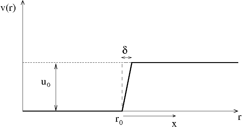
Figure 13: Illustration of replacement of discontinuous step by a finite slope for the square well potential for the purpose of calculating the virial. The limit $\delta\rightarrow 0$ is taken at the end.

The contribution to the time integral of the virial from this event is given by

$$\Delta=\int_{0}^{t_{\delta}}\frac{(r_{0}+x)}{3}Fdt=-\int_{0}^{t_{\delta}}\frac{(r_{0}+x)u_{0}}{3\delta}dt$$ (28)

where $F$ is the (constant) force in the region $0<x<\delta$ and $t_{\delta}$ is the time taken for the ’particle’ (the radial separation) to cross this region. The trajectory $x(t)$ is given by the standard formula for uniform acceleration

$$x(t)=v_{0}t-\frac{1}{2}\frac{u_{0}}{\delta m_{r}}t^{2},$$ (29)

which by setting $x(t_{\delta})=\delta$ gives the following expression for $t_{\delta}$:

$$t_{\delta}=\delta\left(\frac{m_{r}v_{0}}{u_{0}}-\sqrt{\left(\frac{m_{r}v_{0}}{u_{0}}\right)^{2}-\frac{2m_{r}}{u_{0}}}\right);$$ (30)

here we have taken the negative root, appropriate for a positive $u_{0}$ (we want the smallest positive $t_{\delta}$). Returning to $\Delta$, it can be split into two parts as follows

$$\Delta=-\int_{0}^{t_{\delta}}\frac{r_{0}u_{0}}{3\delta}dt-\int_{0}^{t_{\delta}}\frac{x(t)u_{0}}{3\delta}dt$$ (31)

Consider the second term: using the expression for $x(t)$ from Eq. (29), we see that the result of the integral will involve a term proportional to $t_{\delta}^{2}$ and one proportional to $t_{\delta}^{3}$. Using Eq. (30) to replace $t_{\delta}\propto\delta$, and noting the $\delta$ in the denominator, the terms will have linear and quadratic dependence on $\delta$, respectively. Thus they will vanish in the limit $\delta\rightarrow 0$. On the other hand, the first term gives

$$\Delta=-\frac{r_{0}u_{0}}{3\delta}t_{\delta} =-\frac{r_{0}u_{0}}{3}\left(\frac{m_{r}v_{0}}{u_{0}}-\sqrt{\left(\frac{m_{r}v_{0}}{u_{0}}\right)^{2}-\frac{2m_{r}}{u_{0}}}\right)$$

$$=\frac{r_{0}m_{r}}{3}\left(\sqrt{v_{0}^{2}-2u_{0}/m_{r}}-v_{0}\right).$$ (32)

This expression can be simplified by writing it in terms of the change of velocity $\Delta v\equiv v_{1}-v_{0}$. In the one-body problem conservation of momentum does not hold, and $v_{1}$ is given by energy conservation:

$$\frac{1}{2}m_{r}v_{0}^{2}=\frac{1}{2}m_{r}v_{1}^{2}+u_{0}$$ (33)

from which $\Delta v$ is obtained as

$$\Delta v\equiv v_{1}-v_{0}=\sqrt{{v_{0}}^{2}-2u_{0}/m_{r}}-v_{0},$$ (34)

thus the expression for $\Delta$ becomes

$$\Delta=\frac{r_{0}m_{r}}{3}\Delta v=\frac{m_{r}}{3}\mathbf{r}\cdot\Delta\mathbf{v}$$ (35)

where in the last expression a switch to three-dimensional notation was made, recognizing that for central potentials $\Delta\mathbf{v}$ will be parallel to the displacement vector between the two particles. This expression, derived for escape events, must also hold for capture events since these are time-reverses of each other, and the virial is fundamentally a configurational quantity, independent of dynamics (the above expression is time-reversal invariant because the change in the radial component of velocity is the same either way, since although the “initial” and “final” velocities are swapped, they also have opposite sign). Bounce and collision events may be treated by dividing the event into two parts at the turning point (where the relative velocity is zero), noting that each may be treated exactly as above, then adding the results back together. If we now consider all events that take place during an averaging time $t_{\textrm{av}}$), we get the time-averaged virial as

$$\bar{W}=\frac{1}{3t_{\textrm{av}}}\sum_{\textrm{events}\,e}m_{r,e}\mathbf{r}_{e}\cdot\Delta\mathbf{v}_{e}$$ (36)

References

- Landau and Lifshitz (1980) L. D. Landau and E. M. Lifshitz, Statistical Physics, Part I (Pergamon Press, London, 1980).
- Hansen and McDonald (1986) J. P. Hansen and I. R. McDonald, Theory of Simple Liquids (Academic Press, New York, 1986), 2nd ed.
- Reichl (1998) L. E. Reichl, A Modern Course in Statistical Physics (Wiley, New York, 1998), 2nd ed.
- Allen and Tildesley (1987) M. P. Allen and D. J. Tildesley, Computer Simulation of Liquids (Oxford University Press, 1987).
- Bailey et al. (2008) N. P. Bailey, U. R. Pedersen, N. Gnan, T. B. Schrøder, and J. C. Dyre (2008), to appear in J. Chem. Phys.
- Lennard-Jones (1931) J. E. Lennard-Jones, Proc. Phys. Soc. London 43, 461 (1931).
- Weeks et al. (1971) J. D. Weeks, D. Chandler, and H. C. Andersen, J. Chem. Phys. 54, 5237 (1971).
- Ben-Amotz and Stell (2003) D. Ben-Amotz and G. Stell, J. Chem. Phys. 119, 10777 (2003).
- Pedersen et al. (2008a) U. R. Pedersen, N. P. Bailey, T. B. Schrøder, and J. C. Dyre, Phys. Rev. Lett. 100, 015701 (2008a).
- Landau and Binder (2005) D. P. Landau and K. Binder, A Guide to Monte Carlo Simulations in Statistical Physics (Cambridge University Press, 2005), 2nd ed.
- Zaccarelli et al. (2002) E. Zaccarelli, G. Foffi, K. A. Dawson, S. V. Buldyrev, F. Sciortino, and P. Tartaglia, Phys. Rev. E 66, 041402 (2002).
- Berendsen et al. (1995) H. J. C. Berendsen, D. van der Spoel, and R. van Drunen, Comp. Phys. Comm. 91, 43 (1995).
- Lindahl et al. (2001) E. Lindahl, B. Hess, and D. van der Spoel, J. Mol. Mod. 7, 306 (2001).
- (14) Asap, Asap home page, https://wiki.fysik.dtu.dk/asap, URL https://wiki.fysik.dtu.dk/asap.
- Bailey et al. (2006) N. P. Bailey, T. Cretegny, J. P. Sethna, V. R. Coffman, A. J. Dolgert, C. R. Myers, J. Schiøtz, and J. J. Mortensen (2006), eprint cond-mat/0601236.
- Jacobsen et al. (1987) K. W. Jacobsen, J. K. Nørskov, and M. J. Puska, Phys. Rev. B 35, 7423 (1987).
- Jacobsen et al. (1996) K. W. Jacobsen, P. Stoltze, and J. K. Nørskov, Surf. Sci. 366, 394 (1996).
- Pedersen et al. (2008b) U. R. Pedersen, T. Christensen, T. B. Schrøder, and J. C. Dyre, Phys. Rev. E 77, 011201 (2008b).
- Dzugutov (1992) M. Dzugutov, Phys. Rev. A 46, R2984 (1992).
- Kob and Andersen (1994) W. Kob and H. C. Andersen, Phys. Rev. Lett. 73, 1376 (1994).
- Scott et al. (1999) W. R. P. Scott, P. H. Hunenberger, I. G. Tironi, A. E. Mark, S. R. Billeter, J. Fennen, A. E. Torda, T. Huber, P. Kruger, and W. van Gunsteren, J. Phys. Chem. A 103, 3596 (1999).
- Bailey et al. (2004) N. P. Bailey, J. Schiøtz, and K. W. Jacobsen, Phys. Rev. B 69, 144205 (2004).
- Lewis and Wahnström (1994) L. J. Lewis and G. Wahnström, Phys. Rev. E 50, 3865 (1994).
- Berendsen et al. (1987) H. J. C. Berendsen, J. R. Grigera, and T. P. Straatsma, J. Phys. Chem. 91, 6269 (1987).
- Zaccarelli et al. (2004) E. Zaccarelli, F. Sciortino, and P. Tartaglia, J. Phys.: Condens. Matt. 16, 4849 (2004).
- Mahoney and Jorgensen (2000) M. W. Mahoney and W. L. Jorgensen, J. Chem. Phys. 112, 8910 (2000).
- Sciortino (2002) F. Sciortino, Nature Mater. 1, 145 (2002).
- Daw and Baskes (1984) M. R. Daw and M. I. Baskes, Phys. Rev. B 29, 6443 (1984).
- Hansen and McDonald (1969) J. P. Hansen and I. R. McDonald, Liquid and Liquid Mixtures (Butterworths, London, 1969).
- van Gunsteren et al. (1996) W. F. van Gunsteren, S. R. Billeter, A. A. Eising, P. H. Hünenberger, P. Krüger, A. E. Mark, W. R. P. Scott, and I. G. Tironi, Biomolecular Simulation: The GROMOS96 manual and user guide (Hochschulverlag AG an der ETH Zürich, Zürich, Switzerland, 1996).
- Jorgensen et al. (1984) W. L. Jorgensen, J. D. Madura, and C. J. Swenson, J. Am. Chem. Soc. 106, 6638 (1984).
- Esbensen et al. (2002) K. H. Esbensen, D. Guyot, F. Westad, and L. P. Houmøller, Multivariate Data Analysis - In practice (Camo, Oslo, 2002), 5th ed.