.
A study of heuristic guesses for adiabatic quantum computation
Abstract
Adiabatic quantum computation (AQC) is a universal model for quantum computation which seeks to transform the initial ground state of a quantum system into a final ground state encoding the answer to a computational problem. AQC initial Hamiltonians conventionally have a uniform superposition as ground state. We diverge from this practice by introducing a simple form of heuristics: the ability to start the quantum evolution with a state which is a guess to the solution of the problem. With this goal in mind, we explain the viability of this approach and the needed modifications to the conventional AQC (CAQC) algorithm. By performing a numerical study on hard-to-satisfy 6 and 7 bit random instances of the satisfiability problem (3-SAT), we show how this heuristic approach is possible and we identify that the performance of the particular algorithm proposed is largely determined by the Hamming distance of the chosen initial guess state with respect to the solution. Besides the possibility of introducing educated guesses as initial states, the new strategy allows for the possibility of restarting a failed adiabatic process from the measured excited state as opposed to restarting from the full superposition of states as in CAQC. The outcome of the measurement can be used as a more refined guess state to restart the adiabatic evolution. This concatenated restart process is another heuristic that the CAQC strategy cannot capture.
pacs:
03.67.Lx, 03.67.Ac, 03.65.-wI Introduction
Adiabatic quantum computation (AQC) Farhi2000 is a promising paradigm of quantum computation because of its robustness childs01 ; lidar08 , and its intuitive mapping from NP-complete and NP-hard problems to potentially realizable Hamiltonians Farhi2000 ; Farhi2001 ; hogg03 ; young08 . Adiabatic quantum computing is attractive because relevant optimization problems such as lattice models for protein folding can be readily formulated perdomo08 .
AQC algorithms involve the specification of a time-dependent Hamiltonian,
| (1) |
This Hamiltonian has three important functions: (1) The initial Hamiltonian, , encodes a ground state that is easy to prepare and that is used as the initial state for the quantum evolution. (2) The driving Hamiltonian, , is responsible for mediating the transformation of the initial ground state to any of other state. (3) The final Hamiltonian, , is problem dependent and its ground state encodes the solution, , to the computational problem. In the ideal case of a process being fully adiabatic, evolution under will keep the quantum state, , in the ground state of throughout . If this condition is met, the final state at should coincide with the ground state of the final Hamiltonian, , i.e., , if the process is adiabatic. The measurement at will provide the solution to the computational problem.
Since the original proposal by Farhi et al Farhi2000 , a significant amount of progress has been made towards the design of final Hamiltonians for different computationally intractable problems such as NP-complete problems. For example, in this paper we provide a detailed description of the construction of final Hamiltonian for the 3-SAT problem. In previous work, we described the respective construction of the final Hamiltonian for an NP-hard problem of interest in biology, the protein folding problem, which consists of finding the minimum energy configuration of a chain of interacting amino acids in a lattice perdomo08 . Several choices for have been suggested. Farhi et al Farhi2000 proposed what we call in this work the conventional form used for : a linear ramp,
| (2) |
In Farhi et al’s scheme the term can be defined as , namely, the term serves as the initial Hamiltonian when its intensity is completely turned on at , and drives the quantum evolution until it is completely turned off at . The final Hamiltonian is turned on with the functional form . Scheduling the adiabatic evolution with this linear interpolation is not compulsory, thus different proposals have been studied such as the use of non-linear time-profile for auxiliary Hamiltonians farhi_quantum_2002 and optimal geodesic paths rezakhani_quantum_2009 .
The question of whether AQC, or in general quantum computers, can be used for efficiently solving NP-complete problems is a difficult open question. Lessons that have been learned farhi_to_2008 include that a poor choice of the initial Hamiltonian such as the one-dimensional projector as selected in Refs. roland_quantum_2002 and znidaric_exponential_2006 , will lead inefficient AQC algorithms. Therefore, it is important to consider different strategies which might allow an escape from bottlenecks or trap states which might limit the use of AQC amin2008 .
When attempting to tackle combinatorial and optimization problems with classical computers, a common approach to cope with intractability and NP-complete problems garey79 ; sipser05 , is to employ heuristic algorithms as an alternative to exhaustive search which scales exponentially with system size. In quantum computation, Hogg hogg_highly_1998 ; hogg_quantum_2000 introduced heuristic techniques in quantum algorithms. He showed that using information about the structure of the problem as a heuristic guide can be used to enhance the performance of quantum search compared to the scheme proposed by Grover grover_quantum_1997 . Hogg’s proposal was suggested for the gate model for quantum computation, but to our knowledge, there are no studies of heuristics in AQC. The purpose of this paper is to examine the following questions: How can we incorporate heuristics in AQC? Is there any advantage by doing so? What are the modifications to CAQC proposal from an algorithmic and experimental point of view?
Initial state selection.
The simplest form of heuristics we could think of is to start the quantum evolution from a quantum state which is a guess to the solution, but this possibility is not available in any of the proposals for AQC. Physical intuition as well as constraints within the problem can be used to make an educated guess. To illustrate our idea, let’s use a lattice model for protein folding perdomo08 as an example. For this model, an educated guess for the initial state would be to choose a bit string which encodes an initial position for the amino acids in the spatial lattice such that no two amino acids are on top of each other, and that they are connected according to the sequence defining the protein to be folded. Conversely, CAQC would begin the computation with a quantum superposition of all possible states of the computational basis. This choice of initial state contains absurd configurations like all amino acids on top of each other, or assignments referring to configurations of amino acids which are fully disconnected or not properly linked according to the protein sequence. We conjecture here that the presence of these “non-sensical” states might act as trap states, making a smooth transition towards the desired final ground state more difficult and therefore increasing the time required for an adiabatic evolution. In other fields of computer science, physics and chemistry, one might also use classical methods or a mean field approach to find approximate solutions to be employed as educated guesses. For example, in the context of quantum simulation, a Hartree-Fock solution may be used as the initial state for an adiabatic preparation of an exact molecular wave function Aspuru-Guzik2005 ; ward_preparation_2009 ; wang_quantum_2008 ; wang_efficient_2009 .
In quantum mechanics, preparing a desired state is not a trivial task kohen_quantum_1993 ; aharonov_adiabatic_2003 and it is not always possible to deterministically prepare a state from a superposition state by measurement. For NP-complete classical problems, like the 3-satisfiability problem (3-SAT) garey79 ; sipser05 studied here, the simplest guess for the initial state is that of choosing one of the possible assignments from the solution space. We present a strategy which allows to design experimentally-realizable initial Hamiltonians whose ground state corresponds to the desired guess as the initial quantum state. This is essential for studying the importance of choosing a guess state instead of having full superposition of states as in CAQC Farhi2000 . In an algorithm like the one proposed here, both the initial guess and the final solution will be states of the computational basis. Therefore, the overlap between them is zero, unless one has guessed the right solution or the guess is included in the subspace of solutions, which is very unlikely. Regardless of this counterintuitive choice, , we show that using this kind of heuristics can be of advantage. Even in the case of choosing the initial state by random guessing there is potential for outperforming CAQC.
Restarting the evolution.
Notice that the method described here not only allows to begin the evolution from a guess state, but also allows for the possibility of restarting a failed AQC calculation from the measured state. This state can be used as a refined guess to restart the adiabatic evolution. An adiabatic processes is an idealized concept because real experiments have to be run in finite time and therefore there will always be probability of measuring a non-desired excited state which does not encode the solution to the computational task. The possibility of restarting the quantum evolution using the measured state as a guess is a feature which is not available in any of the AQC proposals to date, to our knowledge.
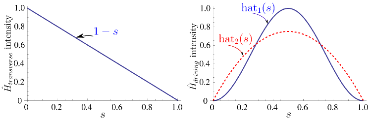
The incorporation of heuristics in AQC essentially involves two modifications to CAQC. We address both changes; the first modification involves the design of initial Hamiltonians for arbitrary guess states. The second modifications involves the change of the time profile of the driving Hamiltonian from the linear ramp to a non-linear time dependence with a “sombrero-like” time profile (see Fig. 1). Note that this second change is not the main point of the paper since non-linear paths had been proposed before farhi_quantum_2002 . Also, it is not our purpose to explore what is the optimal selection for the driving term. It must be emphasized that the “sombrero-like” time profile is an essential feature needed if one is interested in the kind of heuristics we describe here, but this is not the case in the conventional way of doing AQC where it was used for auxiliary Hamiltonian terms farhi_quantum_2002 . Because of this distinctive feature and with the purpose of differentiating our heuristic strategy proposed with CAQC, we will refer to our method as Sombrero Adiabatic Quantum Computation (SAQC). The name should be associated with the algorithmic strategy (selection of initial guess, design of initial Hamiltonian and sombrero-like profile for the driving Hamiltonian) which aims to incorporate heuristics in AQC, not only to the use of non-linear paths in AQC.
The paper is divided as follows: in Section II, we review the CAQC approach. Section III introduces the basic elements of the new implementation, SAQC. Finally, in Section IV, we present numerical calculations comparing the performance of both the CAQC and the SAQC algorithms based on the minimum gap, , of their respective time-dependent Hamiltonians driving their corresponding time evolutions.
II Conventional adiabatic quantum computation (CAQC)
The goal of AQC algorithms is that of transforming an initial ground state into a final ground state , which encodes the answer to the problem. This is achieved by evolving the corresponding physical system according to the Schrödinger equation with a time-dependent Hamiltonian . The AQC algorithm relies on the quantum adiabatic theorem Messiah ; marzlin_inconsistency_2004 ; tong_sufficiency_2007 ; wei2007 ; zhao2008 ; amin_inconsistency_2008 ; mackenzie_validity_2007 ; ambainis_elementary_2004 ; jansen_bounds_2007 ; wu_adiabatic_2007 ; chen_invariant_2007 , which states that if the quantum evolution is initialized with the ground state of the initial Hamiltonian, the time propagation of this quantum state will remain very close to the instantaneous ground state for all , whenever varies slowly throughout the propagation time . This holds under the assumption that the ground state manifold does not cross the energy levels which lead to excited states of the final Hamiltonian. Here, we denote by ground state manifold the first curves associated with the lowest eigenvalue of the time-dependent Hamiltonian for , where is the degeneracy of the final Hamiltonian ground state. An example of , is shown in Fig. 5 of Ref. perdomo08 .
Conventionally the adiabatic evolution path is the linear sweep of , where :
| (3) |
(see Eq. 9 below) is usually chosen such that its ground state is a uniform superposition of all possible computational basis vectors, for the case of an qubit system. Here, we choose the spin states {}, which are the eigenvectors of with eigenvalues +1 and -1, respectively, as the basis vectors. Then the initial ground state is . Such an initial ground state is usually assumed to be easy to prepare, for example, by imposing a global transverse field. Since each state encodes a possible solution, this initial state assigns equal probability to all possible solutions to the computational problem.
III Sombrero adiabatic quantum computation (SAQC)
For SAQC, the time-dependent Hamiltonian can be written as:
| (4) |
We want the non-degenerate ground state of the initial Hamiltonian to encode a guess to the solution, and the driving term, , to couple the states in the computational basis. The function is zero at the beginning and end of the adiabatic path; therefore acts only in the range in a “sombrero-like” time dependence (see Fig. 1), which allows () to be fully turned on at the beginning (end) of the computation.
III.1 Design of the initial Hamiltonian for the guess state
As preparing an arbitrary initial non-degenerate ground state for adiabatic evolution is not a trivial task, we focus on easy to prepare initial guesses that consist of one of the states in the computational basis. The strategy proposed builds initial Hamiltonians such that the initial guess corresponds to the non-degenerate ground state of the initial Hamiltonian, as it is required by AQC. Additionally, this ground state would be non-degenerate.
Let us denote the states of the computational basis of an qubit system as where . The proposed initial Hamiltonian, whose ground state corresponds to an arbitrary initial guess state of the form , can be written as
| (5) |
where each is a boolean variable, , while is a quantum operator acting on the -th qubit of the multipartite Hilbert space . The operator is given by
| (6) |
where is placed in the th position and the identity operators act on the rest of the Hilbert space.
The states constituting the computational basis, and , are eigenvectors of with eigenvalues and , and therefore they are also eigenstates of the operator with eigenvalues 0 and 1 respectively. The logic behind the initial Hamiltonian in Eq. 5 then is clear: if , then but in the case of , then .
As an example, suppose one has a four qubit system, and one wishes to initialize the adiabatic computation with the state which one may choose either randomly or as an educated guess to the solution. According to Eq. 5, the initial Hamiltonian for the guess state should be constructed as
| (7) |
and, clearly
| (8) |
In general, the states of the computational basis are all eigenstates of , and it can be easily verified that the spectrum of are energies contained in . As required, the ground state is also nondegenerate. The other states will have an eigenenergy which equals their Hamming distance to the ground state of the initial Hamiltonian.
III.2 Driving Hamiltonian
The encoding of an educated or a random guess into (Eq. 5) makes both and (Eq. 4) diagonal in the computational basis. Therefore, connecting and with a linear ramp (as in Eq. 3), namely, omitting the operator in the quantum evolution, would yield zero probability of obtaining the state that encodes the unknown solution to the problem starting from the initial guess state. To avoid such a situation, must introduce non-diagonal terms in (see Eq. 4) that allows the initial state to transform from any arbitrary guess into the solution.
In order to make a fair comparison between CAQC and SAQC (see Eq. 3 and Eq. 4), we set
| (9) |
in Eq. 4, where stands for the quantum operator acting on the th qubit of the multipartite Hilbert space . The operator is given by , where the operator has been placed in the th position, and the ’s are identity operators. From a physical point of view, the Hamiltonians and can be related to a transverse magnetic field. The intensity of these Hamiltonians is tuned by varying the parameter. If we set to be the same for both adiabatic algorithms, all the dependence of the transverse field intensity lies on functions in Eq. 3 and in Eq. 4. A reasonable requirement for a fair comparison between CAQC and SAQC is that they both provide the same average intensity of the transverse magnetic field in . A choice of with the same average , is .
Even though nonlinear evolutions have been proposed in previous articles farhi_quantum_2002 ; andrecut2004 ; siu2007 , our hat function can be as simple or as complicated as desired, as long as is fulfilled. There is plenty of room to optimize the performance by choosing a more convenient hat for the adiabatic evolution, we emphasize that the additional advantage of SAQC is the possibility of choosing an initial guess. In the next section we present some results obtained based on one of the simple nonlinear function and discuss the performance of both CAQC and SAQC for random 3-SAT instances.
IV Hamiltonians for 3-SAT, numerical calculations and discussion
In order to provide a proof of concept for SAQC and to test the potential usefulness of both random and educated guesses in adiabatic evolution, we performed a numerical study on hard-to-satisfy 6- and 7-variable instances of the 3-SAT problem and compared our results with the CAQC approach. Let us now provide a succinct introduction to the 3-SAT problem as well as to briefly discuss its relevance in the fields of theoretical and applied computer science.
IV.1 Construction of final Hamiltonians for satisfiability problems and design of numerical calculations
The K-SAT Problem. Let be a set of Boolean variables and their negations . Let us now construct a logical proposition , defined as , where , i.e. P is a conjunction of clauses over the set , where each clause consists of the disjunction of literals. Proposition is a K-SAT instance and the solution of the K-SAT problem, for instance , consists of finding a set of values for those binary variables upon which has been built (i.e. a bitstring), so that replacement of such binary variables for their corresponding binary values makes , namely, proposition is satisfied. 3-SAT is a particular case of K-SAT for K=3.
For example, let us examine the following instance of the 3-SAT problem. Let be a set of binary variables, and therefore the set of literals is . Consider a 3-SAT instance specified by the proposition,
As this example suggests, finding solutions of even a modest 3-SAT instance can become difficult quite easily (in this case, has only one solution: .)
3-SAT is an NP-complete problem garey79 ; sipser05 , as opposed to 2-SAT which can be efficiently solved using a classical computer. Consequently, studying the properties of 3-SAT is an important area of research, not only because a polynomial-time solution to 3-SAT would imply P = NP, but also because 3-SAT (due to its polynomial equivalence with K-SAT) may be used to model problems and procedures in theoretical computer science acharyya2007 as well as in several areas of applied computer science and engineering like artificial intelligence gent99 ; mezard02 .
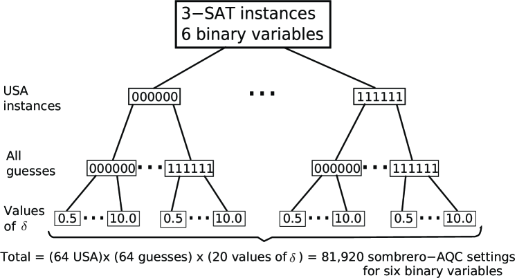
For the purpose of simplifying our discussion, and without loss of generality, we randomly generated 3-SAT instances with a unique satisfying assignment (USA) and their number of clauses to number of variables ratio . This value of corresponds to the phase transition region where hard-to-satisfy instances are expected to be found achlioptas05 ; mezard05 . For completeness and to avoid any kind of bias in selecting this pool of instances, we selected different instances for every variable case studied. More precisely, to exhaustively study the impact of different initial guesses with respect to unique solutions in the behavior of SAQC, we considered all 64 possible initial Hamiltonians (using Eq. 5) for each one of the 64 randomly generated 6-variable USA instances. Similarly, we built 128 initial Hamiltonians for each 7-variable instance, one per possible initial guess (see Fig. 2). The instances were selected in such a way that their solutions had not only a USA, but also that there was no two instances with the same solution.
The generation of our USA 3-SAT instances took several steps, being the first one using the SAT instance generator developed by watanabe . Unfortunately, as this generator does not warranty the production of 3-SAT instances with unique solutions, we took all generated 3-SAT instances and determined, by exhaustive bitstring substitution, whether such instances were USA or not. We iterated this process until we computed all 6-variable and 7-variable 3-SAT instances we needed.
The number of qubits used in our simulations is smaller than state-of-the-art calculations for AQC, such as those carried out by quantum Monte Carlo young08 ; farhi_quantum_2009 . Here we trade off carrying out few large calculations on many qubits for carrying out many calculations on fewer qubits. We wish to answer the question: What is the the impact of the initial guess in the spectral properties of the time-dependent Hamiltonian? To answer this, we explored the space of initial guesses in an exhaustive manner for the case of 6-variable and 7-variable SAT instances. We run a total of 81,920 and 327,680 for 6- and 7- variables respectively (see Fig. 2). As shown in the same figure, we also numerically explored the importance of the strength of the transverse external field for the performance of the algorithm.
Final Hamiltonians are instance-dependent, i.e. the structure of each final Hamiltonian depends on the particular structure (conjunction of clauses) of each 3-SAT USA instance. Our final Hamiltonians comply with the property that it must encode, in its ground state, the solution to the particular 3-SAT USA instance it was designed for Farhi2000 ; znidaric2005a . The design of the final Hamiltonian involves an intermediate step, where a classical cost or energy function is constructed for the particular instance of interest. Once this energy function is expressed in terms of binary variables, it can be easily transformed into a quantum Hamiltonian by performing the mapping indicated by Eq. 6, where each classical binary variable, , is transformed into a quantum operator, . The energy function, , associated with the final Hamiltonian, , can be constructed as a sum of other energy functions, which involve only variables associated with one clause at a time,
| (10) |
Each is designed such that it is equal to 1 if clause is unsatisfied and 0 if the clause is satisfied. Notice that the functions contribute to the count of unsatisfied clauses which defines the spectrum of possible values for , with when all clauses are satisfied.
Formally, suppose is a set of binary variables and their corresponding negations, is a 3-SAT USA instance given by , and each is a disjuction of three elements of , i.e. with and indices are natural numbers, not necessarily consecutive. Finally, let be a set of bits to be substituted in instance . Then, is given by
To construct such a function for any arbitrary clause , it is useful to note that the only assignment for which is when , , and . Therefore, the function by construction, should be 1 when , , and , and 0 otherwise. It can be easily checked that
| (11) |
equals 1 when , , and and 0 otherwise. Recall that each represents a literal and therefore it could be representing the negation of a variable. One can always use the identity to eliminate any , and obtain both and in terms of the .
Consider for example the construction of the energy function required for clause , i.e. is a conjunction of three negated binary variables. In this case, is satisfied by all possible 3-bit bitstrings except for and, according to Eq. 11, the energy function assumes the form .
As a last example consider a clause of the form , where is a conjunction of three non-negated binary variables taken from set . It is clear that will be satisfied by all possible 3-bit bitstrings except for . According to Eq. 11, the energy function for this clause is given by . From the first equality of the previous equation, one can easily check that for all possible 3-bit combinations except for , as expected.
Once we have the final expression for the final classical energy function of Eq. 10, the final Hamiltonians can be obtained using the mapping of Eq. 6, which relates the classical binary variables with quantum operators. Since we selected only USA instances for our study, each has a non-degenerate ground state encoding the unique solution of one of our 3-SAT instances with corresponding ground eigenvalue equal to zero. The final Hamiltonians are the same for both strategies, CAQC and SAQC.
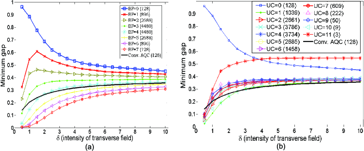
The numerical results on the dependence of the minimum-gap value, , as a function of are shown in Fig. 3. Curves were computed by taking the median of all bit strings that fulfilled the criteria specified in the legend boxes; namely either to produce unsatisfied clauses (UC=) when substituting the initial guess bit string in its corresponding instance, or to be bit flips away from the solution (BF=). BF represents the well known Hamming distance between the solution and the initial guess state. We focused on UC and BF because, in principle, the notion of closeness of an initial guess to the actual solution may be defined with either parameter. Data corresponding to a fixed value of is a statistical representation (median) of typical values that would be expected for hard 3-SAT instances if the guess state belonged to a definite number of UCs or BFs under an experimental setup using SAQC. Such curves are compared with the minimum gap expected for CAQC.
IV.2 Effects of the variation in the transverse field intensity on the minimum energy gap
The dependence of values as a function of the transverse field intensity leaves open some important questions regarding the efficiency of adiabatic quantum algorithms, whether CAQC or SAQC. For example, what is the optimum value of which minimizes the running time of an adiabatic algorithm? How transferable is this optimum value among computational problems? Although we do not intend to do a thorough study of this question in this paper, we would like to give some insight into this question and provide a qualitative discussion of what kind of results might be expected.
Following closely the notation from Farhi et al Farhi2000 , consider , with instantaneous values of defined by
| (12) |
with
| (13) |
where is the dimension of the Hilbert space, and the number of qubits or equivalently the number of binary variables in the SAT instance. According to the adiabatic theorem, if the gap between the two lowest levels, , is greater than zero for all , and taking,
| (14) |
with the minimum gap, , defined by,
| (15) |
and given by,
| (16) |
then we can make the normed overlap
| (17) |
arbitrarily close to 1. In other words, the existence of a nonzero gap guarantees that remains very close to the ground state of for all , if is sufficiently large.
Even though we are aware of the new and more stringent conditions for adiabaticity marzlin_inconsistency_2004 ; tong_sufficiency_2007 ; wei2007 ; zhao2008 ; amin_inconsistency_2008 ; mackenzie_validity_2007 ; ambainis_elementary_2004 ; jansen_bounds_2007 ; wu_adiabatic_2007 ; chen_invariant_2007 and that Eq. 14 is just one of the inequalities to guarantee adiabatic evolution (though there is still lack of a sufficient and necessary condition according to Ref. du2008 ), we will base our discussion on Eq. 14 to illustrate that there is nothing anomalous in employing the additional Hamiltonian term in the full time-dependent Hamiltonian for SAQC. As well as in CAQC, the algorithmic complexity relies again in avoiding an exponentially narrowing of . Along the way we find an important observation about the scaling of the running time as a function of the parameter .
Let us first determine an upper bound for in Eq. 14. Consider the Hamiltonian in Eq. 4 with hat since this was the functional form used for our numerical calculations. We already discussed, at the end of Sec. III.1, that the spectrum of is contained in and, similarly, it can be easily shown that the spectrum of (see Eq. 9) is contained in . On the other hand, the spectrum of the final Hamiltonian, , is instance dependent, and its construction guarantees that the maximum eigenvalue would be which denotes the total number of clauses. This eigenvalue would only appear in case we had an assignment which violates all of the clauses. Using these spectra upper bounds, we can establish an upper bound for in Eq. 14, i.e,
| (18) |
Where we have used the triangle and Schwartz inequality and also the fact that , with close to 4.26 in this particular study. We can see that in the worst case scenario, scales linearly with the number of variables , and linearly with the intensity of the magnetic field, = . A similar analysis gives also that = , and therefore, we showed that for SAQC, not surprisingly, the algorithmic complexity also relies on the scaling of .
An interesting observation arise by analyzing the linear scaling of with and using the numerical results for the dependence of the typical minimum gap values as a function of . There seem to be at least two distinguishable regimes for the dependence of on for both CAQC and SAQC (Fig. 3). For relatively small values of , scales approximately linearly with and therefore . Since the running time is given by Eq. 14, and , the running time decays inversely proportional to within this linear regime. However, for large values of , in the ‘stationary’ regime where is almost constant, increasing field intensity through would make both algorithms less efficient as running time would increase roughly linearly with .
Both CAQC and SAQC would benefit from an increase in the transverse field for small values of , but notice that values for SAQC are more sensitive to , and soon become better on average than those for CAQC (Fig. 3). According to the previous discussion about running time as a function of , it would be ideal to choose near the end of the linear regime; in our calculations, somewhere in the interval (1,2). Further studies concerning the optimum value of as a function of the number of binary variables are needed, but we chose for our analysis on the performance in SAQC and CAQC described in the following section.
IV.3 Performance comparison between SAQC and CAQC
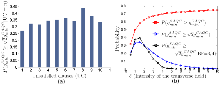
The data sorted with respect to BFs and UCs shows an increase of the minimum gap, , as the Hamming distance from the initial guess to the solution decreases; the trend for UC is less apparent (see Fig. 3). Computing the number of UCs produced by a given initial guess can be done in polynomial time on a classical computer. Unfortunately there is no way to determine a priori how many bit flips the guess is from the solution, as that requires knowledge of the solution itself. Additionally, Fig. 4(a) shows that the SAQC implementation, using as defined in Eq. 9, does not necessarily favor states with low values of UC, but rather gives a homogenously distributed success probability between 25-45%, for . This is in accordance to the observation that solving 3-SAT hard instances is not necessarily guided by minimizing the number of UCs kautz07 . Given the above scenario, we analyzed the likelihood of better performance by choosing initial guesses at random.
In the following discussion, we use the term significantly better initial guess to mean an initial condition that leads a SAQC algorithm to be at least twice as fast as CAQC, i.e. running times for CAQC, , and SAQC, , are such that or, equivalently, , assuming .
For , choosing an initial state at random yields a probability greater than of having (squares) as shown in Fig. 4(b). Moreover, the probability of significantly better performance, i.e. is (triangles). With the intention of predicting the performance of the SAQC protocol in the limit of large , the third curve (circles) was produced using the following rationale: for USA instances, the number of bit configurations with a given value of follows a binomial distribution . In the limit of large , the likelihood of choosing a state in the central region of the binomial distribution is the highest. This observation led us to concentrate on the performance of the most populated instance subsets, those that correspond to BF for 7 variables. Here, the probability of significantly better performance is close to .
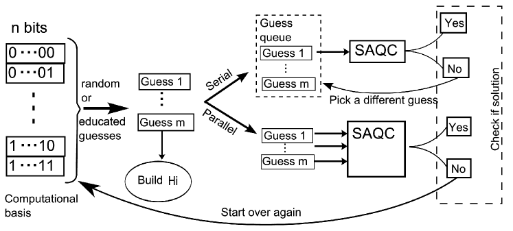
Finally, we propose an algorithm based on SAQC. An initial guess is chosen either at random or by applying expert-domain knowledge and then encoded into the initial ground state of (Eq. 5). An adiabatic passage based on SAQC is then performed either in serial or in parallel, depending on the availability of quantum hardware resources (see Fig. 5.). As an example of the potential usefulness of our algorithm, recall from Fig. 4 that the probability of significantly better performance using SAQC is for .
One way to employ the probabilities we obtained from our numerical simulations in a more concrete scenario is: suppose one is assigned the task of using an adiabatic quantum computer and assume one uses Eq. 14 or any of the more stringent conditions for adiabaticity marzlin_inconsistency_2004 ; tong_sufficiency_2007 ; wei2007 ; zhao2008 ; amin_inconsistency_2008 ; mackenzie_validity_2007 ; ambainis_elementary_2004 ; jansen_bounds_2007 ; wu_adiabatic_2007 ; chen_invariant_2007 to estimate for how long one may need to run an algorithm under the CAQC paradigm. Moreover, suppose that this estimated running time required to remain in the ground state with a high success probability is 2 days. Using the numerical results presented in this paper, one can opt for performing the same task using SAQC as follows: suppose we have absolutely no information about the problem as it was in the case of this numerical study with random 3-SAT USA instances. Instead of running the CAQC algorithm for 2 days, pick a guess state at random from all the possible assignments and then use it as initial state for SAQC and run the algorithm with 1 day. According to Fig. 4, the probability of having picked a state whose performance is as good as CAQC is 39%, for . If after measurement at the end of the first day the result is not a solution, we still can pick another state at random and let it run for one more day. By now the probability of having picked a state with the same performance as the CAQC in the two trials equals 63%. Note that in this simple probability calculations we are not taking into account the fact that even in the case where the state selected for the first run was not one of the ‘ideal’ ones (states corresponding to the 39 % of guesses for the results presented in Fig. 4), we still have a very good chance that the ‘non-ideal’ state still delivers a right answer after the first measurement. This probabability will depend of course on how close is the chosen state from the set of ‘ideal’ ones.
Consequently, the execution of two SAQC algorithms in serial would take at most as much time as the execution of only one CAQC algorithm. By allowing us to choose two guesses to run in the same time as one case in CAQC, the probability of choosing a significantly better initial guess in these two SAQC executions increases from 39% to 63%. Furthermore, even when no significantly better initial guess is chosen and the process is not guaranteed to be fully adiabatic, there is still some probability that we measure the correct solution at the end of both executions.
V Conclusions
In summary, we propose an algorithmic strategy which incorporates heuristics in adiabatic quantum computation. In particular, we study one of the most basic heuristic strategies consisting of initializing the computation with a desired initial state chosen by physical intuition, an educated guess, classical preprocessing of the problem, and/or by randomly choosing one of the possible assignments. This method allows to bridge powerful classical techniques such as heuristic optimization routines and/or mean-field calculations to obtain approximated solutions of the problem and use them as initial guess states for SAQC. The strategy presented allows for a parallel and/or a concatenated scheme. The parallel setup might be helpful if several adiabatic quantum platforms are available in which several guesses can be run simultaneously, one guess to run in each one of the adiabatic processing units. The idea of the concatenated scheme is to restart a failed adiabatic evolution with the measured excited state. Assuming a near-adiabatic trajectory, the measured excited state can be taken as a refined guess from which the quantum evolution is restarted. Notice this is not possible in the conventional approach which would restart the evolution from the full superposition, attributing equal probability to all the states, therefore “erasing” the information gained in the previous near-adiabatic evolution. Neither of the two features proposed above are possible in any of the different adiabatic quantum computation proposals to date. In addition, all the modifications proposed related to different adiabatic paths, auxiliary perturbations farhi02 can also be explored in the context of SAQC, which is also suitable to study quantum problems kempe_complexity_2006 ; bravyi_efficient_2006 ; oliveira_complexity_2008 ; aharonov07 ; mizel07 .
The numerical study performed in this paper is a proof-of-principle to explore the importance and consequences of starting the adiabatic evolution with a guess state and to illustrate that incorporating this kind of heuristics in AQC is possible and might be advantageous. Our numerical simulations show that starting the adiabatic evolution with a guess state which has a zero-overlap with the solution, , is not a big concern. On the contrary, even when there is no hope to make an educated guess and selection of the initial state at random is the only available alternative, we obtain that approximately 40% of states might allow running the quantum algorithm at least twice as fast when compared to CAQC. This possibility of running the algorithm for shorter times but with several trials brings also additional advantages of getting the right answer in any intermediate measure. Moreover, these shorter runs would be less affected by decoherence effects.
Even though the procedure used for the performance comparison, CAQC vs. SAQC, is “reasonable” since it is based on the widely-used minimum gap criteria and its connection with the algorithm run-time (see Eq. 14), we are aware of the limitations of this analysis marzlin_inconsistency_2004 ; tong_sufficiency_2007 ; wei2007 ; zhao2008 ; amin_inconsistency_2008 ; mackenzie_validity_2007 ; ambainis_elementary_2004 ; jansen_bounds_2007 ; wu_adiabatic_2007 ; chen_invariant_2007 . We want to stress that the present numerical results are only encouraging indicators that heuristics in AQC might be a valuable algorithmic strategy for AQC, given the strong dependence of the value of the minimum gap as a function of the initial guess chosen. It is not our purpose to claim superiority of SAQC but to introduce the approach and the motivation behind it. For a more rigorous comparison of both schemes, CAQC and SAQC, we suggest numerical experiments which are not meant to be exhaustive but preferably involving larger size instances, and to explore different problems other than random 3-SAT. For example, we are interested in performing these studies for relevant instances of our recently developed AQC proposal for protein folding perdomo08 and for adiabatic preparation of molecular ground states Aspuru-Guzik2005 where we expect the mean-field (Hartree-Fock) solution to be a better guess than a full superposition. Numerical propagation of the time-dependent Schrödinger equation, instead of inspection of the minimum gap after the Hamiltonian diagonalization, for these cases will provide a realistic simulation of the quantum computation.
Open questions to be explored further is the connections between SAQC, quantum phase transitions schutzhold06 ; latorre_adiabatic_2004 , entanglement ors_universality_2004 and the effect of local minima amin2008 . The performance of the adiabatic algorithm in the limit of large is still an open question farhi_quantum_2009 ; young_2009 which needs to be explored in the context of SAQC. It is not obvious that the same observations and conclusions/observations mentioned above for CAQC will hold for SAQC as well. For example, we think that SAQC might be a strategy to avoid the local minima traps described in Ref. amin2008 . From the study of the spectral properties of the random 3-SAT instances studied, we found that some initial states have a considerably larger gap and while others show a considerably smaller gap when compared with CAQC. Since the initial state in CAQC is a full superposition of all the possible states or solutions, including the ones with a large gap and others with small gap, we conjecture here that having a full superposition will not necessarily be the best choice, given that the presence of the states with small gaps could slow down the quantum evolution. An analysis beyond the gap criteria would be needed to test this conjecture. Solving the time-dependent Schrödinger equation for the entire evolution is the most straightforward, yet numerically-challenging approach. In SAQC, the probability of obtaining these trap states can be avoided and even in the case of a failed evolution, the concatenated scheme may help to restart using a better guess. In contrast, in CAQC, the full superposition including states with considerably small gap might result in a bottleneck for the dynamics towards a successful computation. Further studies need to be done to verify this is indeed the case.
Acknowledgements.
All authors thank E. Farhi and S. Gutmann for useful discussions the led to Fig. 4 and related analysis. S.V.A. gratefully acknowledges P. Grasa and R. Rueda for their support, and Tecnológico de Monterrey Campus Estado de México for funding. A.P. and A.A.G gratefully acknowledge funding from D-Wave Systems and Harvard’s Institute for Quantum Science and Engineering. A.A.G. thanks the Army Research Office under contract W911NF-07-0304.References
- (1) E. Farhi, J. Goldstone, S. Gutmann, and M. Sipser, quant-ph/0001106 (2000).
- (2) A. M. Childs, E. Farhi, and J. Preskill, Physical Review A 65, 012322.
- (3) D. A. Lidar, Physical Review Letters 100, 160506 (2008).
- (4) E. Farhi, J. Goldstone, S. Gutmann, J. Lapan, A. Lundgren, and D. Preda, Science 292, 472 (2001).
- (5) T. Hogg, Physical Review A 67, 022314 (2003).
- (6) A. P. Young, S. Knysh, and V. N. Smelyanskiy, Physical Review Letters 101, 170503 (2008).
- (7) A. Perdomo, C. Truncik, I. Tubert-Brohman, G. Rose, and A. Aspuru-Guzik, Physical Review A 78, 012320 (2008).
- (8) E. Farhi, J. Goldstone, and S. Gutmann, quant-ph/0208135 (2002).
- (9) A. T. Rezakhani, W. Kuo, A. Hamma, D. A. Lidar, and P. Zanardi, Physical Review Letters 103, 080502 (2009).
- (10) E. Farhi, J. Goldstone, S. Gutmann, and D. Nagaj, International Journal of Quantum Information 06, 503 (2008).
- (11) J. Roland and N. J. Cerf, Physical Review A 65, 042308 (2002).
- (12) M. Znidaric and M. Horvat, Physical Review A 73, 022329–5 (2006).
- (13) M. H. S. Amin, Physical Review Letters 100, 130503–4 (2008).
- (14) M. Garey and D. Johnson, Computers and Intractability. A Guide to the Theory of NP-Completeness, W.H. Freeman and Co., NY, 1979.
- (15) M. Sipser, Introduction to the Theory of Computation, PWS Publishing Co., 2005.
- (16) T. Hogg, Physical Review Letters 80, 2473 (1998).
- (17) T. Hogg, Physical Review A 61, 052311 (2000).
- (18) L. K. Grover, Physical Review Letters 79, 325 (1997).
- (19) A. Aspuru-Guzik, A. D. Dutoi, P. J. Love, and M. Head-Gordon, Science 309, 1704 (2005).
- (20) N. J. Ward, I. Kassal, and A. Aspuru-Guzik, The Journal of Chemical Physics 130, 194105 (2009).
- (21) H. Wang, S. Kais, A. Aspuru-Guzik, and M. R. Hoffmann, Physical Chemistry Chemical Physics 10, 5388 (2008).
- (22) H. Wang, S. Ashhab, and F. Nori, Physical Review A 79, 042335 (2009).
- (23) D. Kohen and D. J. Tannor, The Journal of Chemical Physics 98, 3168 (1993).
- (24) D. Aharonov and A. Ta-Shma, Adiabatic quantum state generation and statistical zero knowledge, in Proceedings of the thirty-fifth annual ACM symposium on Theory of computing, pp. 20–29, San Diego, CA, USA, 2003, ACM.
- (25) A. Messiah, Quantum Mechanics (Physics), Dover Publications, 1999.
- (26) K. Marzlin and B. C. Sanders, Physical Review Letters 93, 160408 (2004).
- (27) D. M. Tong, K. Singh, L. C. Kwek, and C. H. Oh, Physical Review Letters 98, 150402 (2007).
- (28) Z. Wei and M. Ying, Physical Review A 76, 024304 (2007).
- (29) Y. Zhao, Physical Review A 77, 032109 (2008).
- (30) M. H. S. Amin, 0810.4335 (2008).
- (31) R. MacKenzie, A. Morin-Duchesne, H. Paquette, and J. Pinel, Physical Review A 76, 044102 (2007).
- (32) A. Ambainis and O. Regev, quant-ph/0411152 (2004).
- (33) S. Jansen, M. Ruskai, and R. Seiler, Journal of Mathematical Physics 48, 102111 (2007).
- (34) J. da Wu, M. sheng Zhao, J. lan Chen, and Y. de Zhang, 0706.0264 (2007).
- (35) J.-L. Chen, M. sheng Zhao, J. da Wu, and Y. de Zhang, 0706.0299 (2007).
- (36) M. Andrecut and M. K. Ali, International Journal of Theoretical Physics 43, 925–931 (2004).
- (37) M. S. Siu, Physical Review A 75, 062337–5 (2007).
- (38) S. Acharyya, Journal on Satisfiability, Boolean Modeling and Computation 4, 33 (2007).
- (39) I. Gent and T. Walsh, Internal report, department of computer science, University of Strathclyde (1999).
- (40) M. Mezard, G. Parisi, and R. Zecchina, Science 297, 812 (2002).
- (41) D. Achlioptas, A. Naor, and Y. Peres, Nature 435, 759 (2005).
- (42) M. Mezard, T. Mora, and R. Zecchina, Physical Review Letters 94, 197205 (2005).
- (43) Watanabe research group of Dept. of Math. and Computing Sciences, Tokyo Inst. of Technology, http://www.is.titech.ac.jp/ watanabe/gensat/.
- (44) E. Farhi, J. Goldstone, D. Gosset, S. Gutmann, H. Meyer, and P. Shor, (2009), arxiv.org/abs/0909.4766.
- (45) M. Žnidaric, Physical Review A 71, 062305.
- (46) J. Du, L. Hu, Y. Wang, J. Wu, M. Zhao, and D. Suter, Physical Review Letters 101, 060403 (2008).
- (47) H. Kautz and B. Selman, Discrete Applied Mathematics 155, 1514 (2007).
- (48) E. Farhi, J. Goldstone, and S. Gutmann, quant-ph/0208135 (2002).
- (49) J. Kempe, A. Kitaev, and O. Regev, SIAM Journal on Computing 35, 1070–1097 (2006).
- (50) S. Bravyi, quant-ph/0602108 (2006).
- (51) R. Oliveira and B. M. Terhal, Quantum Information and Computation 8, 0900 (2008).
- (52) D. Aharonov and A. Ta-Shma, SIAM Journal on Computing 37, 47 (2007).
- (53) A. Mizel, D. A. Lidar, and M. Mitchell, Physical Review Letters 99, 070502 (2007).
- (54) R. Schutzhold and G. Schaller, Physical Review A 74, 060304 (2006).
- (55) J. Latorre and R. Orus, Physical Review A 69, 062302 (2004).
- (56) R. Orus and J. I. Latorre, Physical Review A 69, 052308 (2004).
- (57) A.P. Young, S. Knysh, and V. N. Smelyanskiy, (2009), arXiv:0910.1378v1.