Cosmic microwave background bispectrum on small angular scales

Abstract

This article investigates the non-linear evolution of cosmological perturbations on sub-Hubble scales in order to evaluate the unavoidable deviations from Gaussianity that arise from the non-linear dynamics. It shows that the dominant contribution to modes coupling in the cosmic microwave background temperature anisotropies on small angular scales is driven by the sub-Hubble non-linear evolution of the dark matter component. The perturbation equations, involving in particular the first moments of the Boltzmann equation for photons, are integrated up to second order in perturbations. An analytical analysis of the solutions gives a physical understanding of the result as well as an estimation of its order of magnitude. This allows to quantify the expected deviation from Gaussianity of the cosmic microwave background temperature anisotropy and, in particular, to compute its bispectrum on small angular scales. Restricting to equilateral configurations, we show that the non-linear evolution accounts for a contribution that would be equivalent to a constant primordial non-Gaussianity of order $f_{{}_{\rm NL}}\sim 25$ on scales ranging approximately from $\ell\sim 1000$ to $\ell\sim 3000$.

I Introduction

The cosmic microwave background (CMB) offers a unique window on the physics of the early Universe, and in particular on inflationary models. The angular power spectrum of the CMB anisotropies has been extensively used to set constraints on the shape of the inflationary potentials; see e.g. Ref. Komatsu et al. (2008). The statistical properties of the temperature anisotropies and polarisation depend both on the inflationary period during which they were created and on the physics at play after Hubble-radius crossing and during the recombination. At linear order in metric perturbations, those latter physical processes amount to affect the metric perturbations by a multiplicative transfer function. The characteristic features observed in the temperature anisotropy spectrum originate from the development of acoustic oscillations that this transfer function encodes. The overall amplitude of the metric perturbation and its scale dependence are however determined by the inflationary phase.

At linear order, the calculation of the transfer function - and hence the detailed shape of the temperature power spectra - for generic inflationary models requires the identification of the relevant degrees of freedom during inflation (see e.g. Refs. Bardeen (1980); Mukhanov et al. (1992); Sasaki and Stewart (1996)), as well as a full resolution of the dynamics up to recombination time. All these aspects are now fully understood (see e.g. Refs. Uzan and Peter (2005); Bernardeau (2007) and references therein).

At this level of description, the metric perturbations are linearised so that the non-linear couplings that are inherently present in the Einstein equations are ignored. Therefore models that predict Gaussian initial metric fluctuations are expected to induce cosmic fields with Gaussian statistical properties. This is a priori the case for generic models of inflation. It has to be contrasted to models with active topological defects - such as cosmic strings - that have soon been recognised as a source of large non-Gaussianities Pen et al. (1994); Gangui and Mollerach (1996); Durrer et al. (2000); Perivolaropoulos (1993). The current data however clearly favor only mild non-Gaussianities although those might be larger than those induced by pure gravity couplings. This is not the case for single field slow-roll inflation for which it has been unambiguously shown in Ref. Maldacena (2003) that it can produce only very weak non-Gaussian signals, that are bound to be overridden by the gravity induced couplings. It has however been realised that some models of inflation might produce significant deviation from Gaussianity in the context of multiple-field inflation Komatsu (2002); Bartolo et al. (2002); Bernardeau and Uzan (2002, 2003); Lyth and Wands (2002); Bartolo et al. (2004a, b); Bernardeau et al. (2006); Bernardeau and Uzan (2004) or with non-standard kinetic terms Alishahiha et al. (2004). The question of the observation of primordial non-Gaussianities is largely open.

In general however, primordial deviations from Gaussianity are in competition with the couplings induced during the non-linear evolution of the cosmic fields. It has triggered general studies aiming at characterising the bispectrum to be expected in the observation of the cosmic microwave background temperature anisotropies and polarisations whether it arises from inflation or from subsequent effects.

This task is multi-fold. It requires a proper identification of the mode couplings (at the quantum level) during the inflationary phase - so taking into account the usual gauge freedom - as well as a second order treatment of the post-inflationary evolution. While the former has been set on firm ground Maldacena (2003); Weinberg (2005), the latter issue is still largely unexplored. This article proposes both numerical and analytical insights into it.

Hereafter, we assume that on super-Hubble scales, the only significant scalar perturbations are adiabatic and that they obey a nearly Gaussian statistics . To be more precise, they are described in Fourier space by a single variable $\zeta_{0}(\textbf{k})$, k being a comoving wave-number, that satisfies

$$\langle\zeta_{0}(\textbf{k}_{1})\zeta_{0}(\textbf{k}_{2})\rangle=\delta_{\rm D}(\textbf{k}_{1}+\textbf{k}_{2})\ P_{\zeta}(k_{1})$$ (1)

and

$$\langle\zeta_{0}(\textbf{k}_{1})\zeta_{0}(\textbf{k}_{2})\zeta_{0}(\textbf{k}_{3})\rangle=2\delta_{\rm D}(\textbf{k}_{1}+\textbf{k}_{2}+\textbf{k}_{3})\ f_{{}_{\rm NL}}^{\zeta}(\textbf{k}_{1},\textbf{k}_{2})P_{\zeta}(k_{1})P_{\zeta}(k_{2})+{\hbox{sym.}}\ ,$$ (2)

where “sym.” stands for the two other terms obtained by permutation of the wave-numbers. This defines the primordial power spectrum $P_{\zeta}(k)$ and the primordial mode coupling amplitude  $f_{{}_{\rm NL}}^{\zeta}$. Considering an observable quantity $\theta$ related to the perturbation variables, the effect of evolution can generically be recapped  as

$$\theta(\textbf{k}) = {\cal T}_{\theta}^{(1)}(k)\,\zeta_{0}(\textbf{k})+\int\frac{{\rm d}^{3}\textbf{k}_{1}{\rm d}^{3}\textbf{k}_{2}}{(2\pi)^{3/2}}\,\delta_{\rm D}(\textbf{k}\!-\!\textbf{k}_{1}\!-\!\textbf{k}_{2}){\cal T}_{\theta}^{(2)}(\textbf{k}_{1},\textbf{k}_{2})\,\zeta_{0}(\textbf{k}_{1})\zeta_{0}(\textbf{k}_{2})+\dots\ ,$$ (3)

where ${\cal T}_{\theta}^{(1)}(k)$ is the linear transfer function and ${\cal T}_{\theta}^{(2)}(\textbf{k}_{1},\textbf{k}_{2})$ is the second order transfer function. $\theta$ can be thought as being e.g. the observed temperature anisotropies, but it could also stand for the CMB polarisation, or even cosmic shear surveys. When computing the bispectrum of $\theta$ there will be a contribution from the mode couplings induced by the second order transfer function ${\cal T}^{(2)}$ and the possible initial non-Gaussianities,

$$\langle\theta(\textbf{k}_{1})\theta(\textbf{k}_{2})\theta(\textbf{k}_{3})\rangle = 2\delta_{\rm D}(\textbf{k}_{1}+\textbf{k}_{2}+\textbf{k}_{3})\left[f_{{}_{\rm NL}}^{\zeta}(\textbf{k}_{1},\textbf{k}_{2})+f_{{}_{\rm NL}}^{\theta}(\textbf{k}_{1},\textbf{k}_{2})\right]{\cal T}_{\theta}^{(1)}(k_{1}){\cal T}_{\theta}^{(1)}(k_{2}){\cal T}_{\theta}^{(1)}(k_{3})\ P_{\zeta}(k_{1})P_{\zeta}(k_{2})$$ (4)

$$\qquad\qquad+{\hbox{sym.}}$$

where $f_{{}_{\rm NL}}^{\theta}$ is related to the second order transfer function by

$${\cal T}_{\theta}^{(2)}(\textbf{k}_{1},\textbf{k}_{2})\equiv f_{{}_{\rm NL}}^{\theta}(\textbf{k}_{1},\textbf{k}_{2})\,{\cal T}_{\theta}^{(1)}(|\textbf{k}_{1}+\textbf{k}_{2}|)\ .$$ (5)

The full derivation of the details of ${\cal T}_{\theta}^{(2)}$ is a fantastic task. It requires an understanding of the metric fluctuations behaviour at second order, from radiation dominated super-Hubble scales to matter dominated era at sub-Hubble scale, as well as a comprehension of the physics of recombination - through the Boltzmann equation - at a similar order. Such a task has been undertaken by several authors  and the multitude of effects at play needs to be sorted out. So, the goal of this article is not to provide an end to end calculation of ${\cal T}_{\theta}^{(2)}$, but to show that on small scales one can extract the dominant terms in order to get an insight into this physics at second order.

Modes coupling due to gravitational clustering is, by far, not a novel subject. It can be traced back to early works by Peebles Peebles (1980) where the function ${\cal T}^{(2)}$ for the non-linear sub-Hubble evolution of cold dark matter field (CDM) during a matter dominated era was derived. General modes coupling effects, within the same regime, has been extensively studied in the eighties and nineties where a whole corpus of results has been obtained (see e.g. Ref. Bernardeau et al. (2002) for an exhaustive review). On sub-Hubble scales, the second order mode coupling function for the gravitational potential reads

$$f_{{}_{\rm NL}}^{\Phi}(\textbf{k}_{1},\textbf{k}_{2})=\frac{k_{1}^{2}\,k_{2}^{2}}{\frac{3}{2}\,H^{2}\,a^{2}\,|\textbf{k}_{1}+\textbf{k}_{2}|^{2}}$$

$$\quad\times\left(\frac{5}{7}+\frac{1}{2}\frac{\textbf{k}_{1}\cdot\textbf{k}_{2}}{k_{1}^{2}}+\frac{1}{2}\frac{\textbf{k}_{1}\cdot\textbf{k}_{2}}{k_{2}^{2}}+\frac{2}{7}\frac{(\textbf{k}_{1}\cdot\textbf{k}_{2})^{2}}{k_{1}^{2}k_{2}^{2}}\right)$$ (6)

in the particular case of an Einstein-de Sitter universe (here $a$ is the scale factor and $H$ the Hubble parameter). This well-established result proved to be useful for observational cosmology. The angular modulation it exhibits has indeed been observed in actual data sets; see e.g. Ref. Scoccimarro et al. (2001).

The fact that on sub-Hubble scales, that is $k^{2}\gg H^{2}\,a^{2}$, the non-Gaussianity is driven by the non-linearities of the CDM sector, and that they can start developing even before equality is one of the leading ideas of the present study. Indeed temperature anisotropies on small angular scales – i.e. beyond the first acoustic peak – mostly trace the gravitational potential  long after it has entered a sub-Hubble evolution and already during the matter dominated era. It is then natural to expect that the temperature anisotropies should be substantially determined by a form close to that of Eq. (I).

The goal of this paper is to evaluate how close we are from the behaviour (I) depending on scales, to which extent the temperature anisotropies trace this form and finally to estimate the amplitude of the temperature bispectrum on small angular scales. In this work two approaches will be compared: a full numerical integration of the second-order equations presented in § II, where the main approximation lies in the modelisation of the Compton scattering collision term at second order, see Eq. (30), and an approximate analytical resolution discussed in § III.

The bottom line of our analysis is that on small angular scales, the density perturbation of the cold dark matter starts to dominate the Poisson equation so at the time of decoupling we can assume that the system is split in (1) the evolution of CDM and (2) the evolution of the photons-baryons plasma which develops acoustic oscillations in the gravitational potential determined by the CDM component. As we shall demonstrate, at second order the dominant term of the temperature fluctuations is driven by the second order gravitational potential. Our approximation requires to consider a regime in which the Silk damping is efficient, that is wave-modes larger than the damping scales, hence corresponding to multipoles roughly larger that 2000. This picture will be shown to be in agreement with the numerical estimation (see § III.4). We then proceed in § IV by a computation of the bispectrum in which we show that, for equilateral configurations, the non-linear dynamics has an amplitude equivalent to that of a primordial non-Gaussianity with constant $f_{{}_{\rm NL}}$ of order 25. A back-of-the-envelop argument allows us to understand the magnitude of this number.

II Perturbation theory

This section is devoted to the presentation of the perturbation equations, up to second order, and of the initial conditions used in our study. We set the main notation and describe the background dynamics in § II.1, and we define the perturbation variables in § II.2. The perturbation equations and initial conditions are then presented in § II.3 and II.4 respectively.

II.1 The background dynamics

The background space-time is described by a Friedmann-Lemaître metric with scale factor $a$ and cosmic time $t$. It is convenient to rescale the scale factor such that

$$y\equiv\rho_{\rm m}/\rho_{\rm r}\ ,$$

where $\rho_{\rm m}$ and $\rho_{\rm r}$ are the background matter and radiation energy densities respectively. The matter energy density can be decomposed as the sum of a cold dark matter component, that does not interact with normal matter, and a baryonic component, that can be coupled to radiation by Compton scattering prior to decoupling. We thus set $\rho_{\rm m}=\rho_{\rm c}+\rho_{\rm b}$ where $\rho_{\rm c}$ and $\rho_{\rm b}$ refers to CDM and baryons respectively. It follows that

$$\rho_{\rm m}=\frac{\rho_{\rm c}}{1-f_{{}_{\rm b}}}$$

with $f_{{}_{\rm b}}\equiv\Omega_{{\rm b}0}/\Omega_{{\rm m}0}\approx 0.18$. The Friedmann equation then takes the simple form

$$\mathcal{H}^{2}=\mathcal{H}_{\mathrm{eq}}^{2}\frac{1+y}{2y^{2}}$$ (7)

when we neglect the contributions of the spatial curvature and of the cosmological constant, which are negligible for the whole history of the Universe but very recently. $\mathcal{H}\equiv a^{\prime}/a$ is the conformal Hubble parameter and a prime refers to a derivative with respect to the conformal time $\eta$ defined by ${\rm d}t=a{\rm d}\eta$. $\mathcal{H}_{\mathrm{eq}}$ is the value of the $\mathcal{H}$ at equality, that is when $y=1$.

The equation of state of the background fluid, composed of a mixture of non-relativistic matter and radiation, is $w=1/[3(1+y)]$ and the density parameters of matter and radiation are

$$\Omega_{\rm m}=\frac{y}{1+y},\quad\Omega_{\rm r}=\frac{1}{1+y}\$$ (8)

and indeed $\Omega_{\rm c}=\Omega_{\rm m}(1-f_{{}_{\rm b}})$.

Equality takes place at $y=1$, from which we deduce that

$$y_{0}=1+z_{\mathrm{eq}}=3612\,\Theta_{2.7}^{-4}\left(\frac{\Omega_{{\rm m}0}h^{2}}{0.15}\right),$$ (9)

where $\Theta_{2.7}\equiv T_{0}/2.7$ K is the temperature of the CMB today, and $h$ the value of the Hubble constant in units of 100 km/s/Mpc. Equation (7) evaluated today implies that $\mathcal{H}_{\mathrm{eq}}\sim\mathcal{H}_{0}\sqrt{2y_{0}}$ so that

$$\mathcal{H}_{\mathrm{eq}}\sim 0.072\ \Omega_{{\rm m}0}h^{2}\,\mathrm{Mpc}^{-1}.$$ (10)

The last scattering surface corresponds to a redshift Komatsu et al. (2008)

$$1+z_{\mathrm{LSS}}=1090\pm 1=y_{0}/y_{\mathrm{LSS}},$$ (11)

and is mildly dependent of $\Omega_{{\rm c}0}$ and $\Omega_{{\rm b}0}$. This implies that $y_{\mathrm{LSS}}\sim 3.3$.

In Fourier space, a mode is super-Hubble when $k\eta\ll 1$ and sub-Hubble otherwise. The mode becoming sub-Hubble at equality corresponds to a comoving wavelength of

$$k_{\mathrm{eq}}^{-1}=\mathcal{H}_{\mathrm{eq}}^{-1}=\frac{14}{\Omega_{{\rm m}0}h^{2}}\,\mathrm{Mpc}$$ (12)

if we choose units such that $a_{0}=1$.

We also introduce the parameter

$$R=\frac{3}{4}\frac{\rho_{\rm b}}{\rho_{\rm r}}=\frac{3}{4}f_{{}_{\rm b}}\ y\ ,$$ (13)

which will be useful to describe the physics of the baryons-photons plasma.

II.2 Perturbation variables

We focus on the dynamics of scalar perturbations (see e.g. Refs Osano et al. (2007); Lu et al. (2008); Baumann et al. (2007) for analysis of vector and tensor modes generation at second order). In Newtonian gauge, we can expand the metric as

$${\rm d}s^{2}=a^{2}(\eta)\left[-(1+2\Phi){\rm d}\eta^{2}+(1-2\Psi)\delta_{ij}{\rm d}x^{i}{\rm d}x^{j}\right]\,,$$ (14)

where $\Phi$ and $\Psi$ are the two Bardeen potentials.

The various fluids contained in the universe will be described at the perturbation level by their density contrast $\delta$ and their velocity field. For the latter, we decompose the time-like tangent vector to the fluid worldlines according to

$$u^{\mu}=\frac{1}{a}(\delta^{\mu}_{0}+v^{\mu})\ ,$$

where the first term accounts for the background Hubble flow. The perturbation $v^{\mu}$ is further decomposed as $v^{\mu}=(v^{0},v^{i})$ with $v^{i}=\partial^{i}v$ and $v^{0}$ is constrained by the normalisation $u_{\mu}u^{\mu}=-1$.

When dealing with perturbations beyond first order, we assume that the perturbation variables are expanded according to

$$X=X^{(1)}+\frac{1}{2}X^{(2)}\,,$$ (15)

where $X^{(1)}$ satisfies the first order field equations while the second order equations will involve purely second order terms, e.g. $X^{(2)}$ as well as terms quadratic in the first-order variables, e.g. $[X^{(1)}]^{2}$. Thus, there shall never be any ambiguity about the order of perturbation variables involved as long as we know the order of the equation considered, and consequently we will usually omit the superscprit $(1)$ or $(2)$ which specifies the order of the perturbation. For a general discussions on second order perturbations and gauge issues, we forward to Refs. Pitrou (2007); Nakamura (2007); Bruni et al. (1997)

II.3 Perturbation equations

In this article we shall focus on the CDM-radiation-baryons system. Each component has a constant equation of state, that is $P=w\rho$ with $w^{\prime}=0$ so that $c_{s}^{2}=w$. Non-relativistic matter is described by a pressureless fluid with $w_{\rm m}=w_{\rm b}=w_{\rm c}=0$ and radiation satisfies $w_{\rm r}=\frac{1}{3}$.

In full generality, the evolution of each component can be obtained from the Boltzmann equation satisfied by the distribution function $f_{a}(x^{\mu},p_{\nu})$ for this matter component. The stress-energy tensor can then be defined by integrating over momentum as

$$T^{\mu\nu}_{a}(x^{\alpha})=\int f_{a}(x^{\alpha},p_{\beta})\,p^{\mu}p^{\nu}\pi_{+}(p)\ ,$$

where $\pi_{+}(p)$ is the volume element on the tangent space in $x^{\alpha}$ such that $p^{\mu}$ is non-spacelike and future directed (see e.g. Refs Uzan (1998); Pitrou (2007))

The first moment of the Boltzmann equation then gives a conservation equation of the form Uzan (1998)

$$\nabla_{\mu}T^{\mu\nu}_{a}=F^{\nu}_{a}\ ,$$ (16)

where $F^{\nu}_{a}$ describes the force acting on the fluid labelled by $a$ and satisfy $F^{\nu}_{a}u_{\nu}=0$ and $\sum_{a}F^{\nu}_{a}=0$, which is nothing but the action-reaction law (equivalently obtained from the Bianchi identity). Projecting along and perpendicular to $u^{\mu}$, we can extract respectively the continuity and Euler equations.

II.3.1 Linear order

Linear order calculations are used in particular to set the source terms of the second order equations. We closely follow the standard calculations and the main ingredients are recalled here. At linear order, the continuity equation for a fluid labelled by $a$ takes the form Uzan and Peter (2005); Bernardeau (2007); Mukhanov et al. (1992)

$$\delta_{a}^{\prime}+3\mathcal{H}(c_{s,a}^{2}-w_{a})\delta_{a}+(1+w_{a})\left(\Delta v_{a}-3\Psi^{\prime}\right)=0\ ,$$ (17)

while the Euler equation

$$v_{a}^{\prime}+\mathcal{H}(1-3c_{s,a}^{2})v_{a}+\Phi+\frac{c_{s,a}^{2}}{1+w_{a}}\delta_{a}=\mathcal{F}_{a}-\frac{1}{6}\Delta\pi_{a}\ ,$$ (18)

where $\pi_{a}$ is the contribution of the anisotropic pressure. In deriving Eq. (18), we have decomposed the force term as $F_{i}=\partial_{i}F=\partial_{i}[(\rho+P)\mathcal{F}]$ and $F_{0}=0$. Since $F^{\mu}_{a}$ vanishes at the background level, $\mathcal{F}_{a}$ is gauge invariant. $w_{a}$ and $c_{s,a}$ are respectively the equation of state and sound speed of the component $a$.

In our analysis, we consider three components. Dark matter (label ${\rm c}$) is described by a perfect fluid with $w_{\rm c}=0$ and $\pi_{\rm c}=0$ interacting only through gravity ($\mathcal{F}_{\rm c}=0$). Baryons and photons are coupled through Compton scattering so that $\mathcal{F}_{\rm b}$ and $\mathcal{F}_{\rm r}$ do not vanish. The action-reaction law (or equivalently the conservation of the total stress-energy tensor of matter) implies that $F_{\rm r}=-F_{\rm b}$, from which we deduce that

$$\mathcal{F}_{\rm r}=-R\mathcal{F}_{\rm b}\ .$$ (19)

At linear order, it is easily shown that

$$\mathcal{F}_{\rm r}=\tau^{\prime}(v_{\rm b}-v_{\rm r})\ ,$$ (20)

where

$$\tau^{\prime}\equiv an_{e}\sigma_{T}\ ,$$ (21)

with $n_{e}$ being the free electrons number density and $\sigma_{T}$ the Thomson scattering cross-section. It follows that baryons will be described by a fluid ($w_{\rm b}=0=\pi_{\rm b}=0$) interacting with radiation. In general radiation enjoys a non-vanishing anisotropic pressure ($\pi_{\rm r}\not=0$) and should actually be describe by the full Boltzmann hierarchy. For the linear order calculations we choose to extend the fluid description by including the eight first moments of this hierarchy, including polarisation (see Appendix A for these equations). Our choices for the modelisation of the matter sector are summarised in table 1.

Component	$w$	$\mathcal{F}$	$\pi$	description
CDM (${\rm c}$)	0	0	0	fluid
Baryons (${\rm b}$)	0	$\mathcal{F}_{\rm b}$	0	fluid
Photons (${\rm r}$)	$\,\,\frac{1}{3}\,\,$	$\,\,\mathcal{F}_{\rm r}\,\,$	$\,\,\pi_{\rm r}\,\,$	kinetic
				(8 moments)

Table 1: Summary of the properties and descriptions of the matter components considered in our analysis.

The Einstein equations reduce to the set

$$\Delta\Psi-3\mathcal{H}\Psi^{\prime}-3\mathcal{H}^{2}\Phi-\frac{3}{2}\mathcal{H}^{2}\sum_{a={\rm r},{\rm m}}\Omega_{a}\delta_{a}=0\ ,$$ (22)

$$\Psi^{\prime\prime}+\mathcal{H}^{2}\Phi+\frac{1}{3}\Delta(\Phi-\Psi)+\mathcal{H}\Phi^{\prime}+2\mathcal{H}\Psi^{\prime}$$

$$\quad\quad\quad+2\mathcal{H}^{\prime}\Phi-\frac{1}{2}\mathcal{H}^{2}\Omega_{\rm r}\delta_{\rm r}=0\ ,$$ (23)

$$\Psi-\Phi=\Omega_{\rm r}\mathcal{H}^{2}\pi_{\rm r}\ ,$$ (24)

$$\Psi^{\prime}+\mathcal{H}\Phi+\frac{3}{2}\mathcal{H}^{2}\sum_{a={\rm r},{\rm m}}\Omega_{a}(1+w_{a})v_{a}=0\ .$$ (25)

When the anisotropic pressure can be neglected, and in particular in the tight coupling regime discussed below, Eq. (24) implies that $\Phi=\Psi$. Note that in this analysis we actually ignore the neutrinos the effect of which is thought to be marginal on the qualitative results we will obtain.

II.3.2 Second order

At second order, any first order equation, schematically written as $\mathcal{D}[X^{(1)}]=0$, of the first order perturbation variables $X^{(1)}$ will take the general form

$$\mathcal{D}[X^{(2)}]=S$$

where $S$ is a source term quadratic in the first order variables.

For the continuity and Euler equations respectively read

$$S_{c,a} = 2(1+w_{a})\left\{6\Psi\Psi^{\prime}-\Phi\Delta v_{a}-\partial_{i}v_{a}\left[(1-3c_{s,a}^{2})\mathcal{H}\partial^{i}v_{a}+2\partial^{i}v_{a}^{\prime}+2\partial^{i}\Phi-3\partial^{i}\Psi\right]\right\}$$ (26)

$$+2(1+c_{s,a}^{2})\left[3\delta_{a}\Psi^{\prime}-\partial_{i}(\partial^{i}v_{a}\delta_{a})\right]+\frac{(c_{s,a}^{2})^{\prime}}{1+w_{a}}\delta_{a}^{2}\ ,$$

$$\partial_{i}S_{e,a} = -2\frac{1+c_{s,a}^{2}}{1+w_{a}}\left[(\delta_{a}\partial_{i}v_{a})^{\prime}+\mathcal{H}(1-3w_{a})\delta_{a}\partial_{i}v_{a}+\delta_{a}\partial_{i}\Phi\right]+2\mathcal{H}(1-3c_{s,a}^{2})(\Phi+2\Psi)\partial_{i}v_{a}$$ (27)

$$+2\Phi\partial_{i}v_{a}^{\prime}+4\Phi\partial_{i}\Phi+10\Psi^{\prime}\partial_{i}v_{a}+4\Psi\partial_{i}v_{a}^{\prime}-2\partial_{j}\left(\partial^{j}v_{a}\partial_{i}v_{a}\right)+2\frac{(c_{s,a}^{2})^{\prime}}{1+w_{a}}\left[\frac{\delta_{a}\partial_{i}\delta_{a}}{3\mathcal{H}(1+w_{a})}-\delta_{a}\partial_{i}v_{a}\right]\ .$$

As long as CDM is concerned, these source terms and Eqs. (17-18) gives the full second order evolution of the fluid. As already seen at first order, the fluid equations for the baryons and photons must include interaction terms, that is $\mathcal{F}^{(2)}_{\rm r}$ and $\mathcal{F}^{(2)}_{\rm b}$, that derive from the Compton scattering collision term entering the Boltzmann equation for the radiation.

In the baryon rest-frame, this collision term includes only two types of contributions Bartolo et al. (2006); Dodelson and Jubas (1995); Pitrou (2008). First, there is a term involving first order perturbation quantities and whose form is

$$\frac{1}{2}C^{(2)}\propto C^{(1)}\left(\frac{\delta n_{e}}{n_{e}}+\frac{\partial x_{e}}{\partial T}\frac{\delta T^{(1)}}{x_{e}}\right)\ ,$$ (28)

where $C^{(1)}$ is the first order collision term. This contribution involves the fluctuation of the visibility function, that is of the electron density $n_{e}$ and of the ionisation fraction $x_{e}$. It accounts for the fact that a hotter or denser region decouples later. Its typical magnitude is of order $4C^{(1)}\delta n_{e}/n_{e}$. Second, there is a term involving second order perturbation variables and whose form is

$$\frac{1}{2}C^{(2)}\propto C^{(1)}\left[X^{(2)}\right]\ .$$ (29)

The forces derived from these two terms will satisfy by construction the action-reaction law (19), and this holds in any reference frame and at any order. This explains why the computation is easily carried out in the baryons rest-frame Pitrou (2008).

Then, when changing frame from the baryons rest-frame to the cosmological frame, where the computations are actually carried out, a second series of terms appears. They are of the form $\tau^{\prime}f^{(0)}\times[v^{(1)}]^{2}$ and $\tau^{\prime}f^{(1)}\times[v^{(1)}]$, where $f^{(0)}$ and $f^{(1)}$ are the background and first order distribution functions as well as similar terms for the polarisation (see Ref. Pitrou (2008) for the exact form of these terms.).

Now, the contribution (28) is proportional to the collision term at first order. This implies that it will thus be negligible as long as tight coupling between baryons and photons is maintained at first order, i.e. as long as $\tau^{\prime}/k\gg 1$. We are thus left only with the contribution (29). This term thus enforces the tight coupling regime at second order. Then, as long as tight coupling is effective, it is obvious that the second series of terms arising from the change of frames should compensate each other to give a vanishing contribution. We shall thus model the interaction term entering the Euler equations by

$$\mathcal{F}^{(2)}=\mathcal{F}^{(1)}[X^{(2)}]\ ,$$ (30)

that is by assuming that it keeps the same functional form as at first order. In conclusion, the continuity and Euler equations for baryons and photons with the interaction term (30) are the exact fluid limit of the full Boltzmann equation at second order as long as tight coupling is effective. This implies that at second order, and similarly as at first order, the two tightly coupled fluids are equivalent to a single perfect fluid; see section III.1. Again, this stems from the action-reaction law which implies that Eq. (19) has to hold at any order and in any reference frame and that there cannot appear any external force acting on the resulting effective fluid since it is only coupled to other matter components through gravitation.

When $\tau^{\prime}/k$ becomes of order unity, tight coupling stops being effective. But thanks to Silk damping, the terms of the form $\tau^{\prime}f^{(0)}\times[v^{(1)}]^{2}$ and $\tau^{\prime}f^{(1)}\times[v^{(1)}]$, will still be negligible compared to the one we kept to obtain Eq. (30).

Let us now turn to the Einstein equations (22-25). Their source terms read respectively

$$S_{1} = -8\Psi\Delta\Psi-3\partial_{i}\Psi\partial^{i}\Psi-3\Psi^{\prime 2}+3\mathcal{H}^{2}\sum_{a={\rm r},{\rm c},{\rm b}}\Omega_{a}(1+w_{a})\partial_{i}v_{a}\partial^{i}v_{a}-12\mathcal{H}^{2}\Psi^{2}\ ,$$ (31)

$$S_{2} = 4\mathcal{H}^{2}\Psi^{2}+\frac{7}{3}\partial_{i}\Psi\partial^{i}\Psi+\frac{8}{3}\Psi\Delta\Psi+8\mathcal{H}\Psi\Psi^{\prime}+8\mathcal{H}^{\prime}\Psi^{2}+\Psi^{\prime 2}+\mathcal{H}^{2}\sum_{a={\rm r},{\rm c},{\rm b}}\Omega_{a}(1+w_{a})\partial_{i}v_{a}\partial^{i}v_{a}\ ,$$ (32)

$$S_{3} = -4\Psi^{2}-\Delta^{-1}\left[2\partial_{i}\Psi\partial^{i}\Psi+3\mathcal{H}^{2}\sum_{a={\rm r},{\rm c},{\rm b}}\Omega_{a}(1+w_{a})\partial_{i}v_{a}\partial^{i}v_{a}\right]$$ (33)

$$\qquad\qquad\qquad\qquad+3(\Delta\Delta)^{-1}\partial_{i}\partial_{j}\left[2\partial^{i}\Psi\partial^{j}\Psi+3\mathcal{H}^{2}\sum_{a={\rm r},{\rm c},{\rm b}}\Omega_{a}(1+w_{a})\partial^{i}v_{a}\partial^{j}v_{a}\right]\ ,$$

$$S_{4} = 2\mathcal{H}\Psi^{2}-4\Psi\Psi^{\prime}+2\partial_{i}^{-1}(\Psi^{\prime}\partial_{i}\Psi)+3\mathcal{H}^{2}\sum_{a={\rm r},{\rm c},{\rm b}}\Omega_{a}\partial_{i}^{-1}\left[(1+w_{a})\Psi\partial_{i}v_{a}-(1+c_{s,a}^{2})\delta_{a}\partial_{i}v_{a}\right]\ .$$ (34)

This provides all the source terms appearing at second order.

II.3.3 Note on our conventions

Since the first and second order equations are conveniently solved in Fourier space, the quadratic terms in the source terms can be written as a convolution on the wave-numbers $\mathbf{k}_{1}$ and $\mathbf{k}_{2}$ such that $\mathbf{k}_{1}+\mathbf{k}_{2}=\mathbf{k}$. For simplicity of notations we will write the integral factor of the convolution as

$$\mathcal{C}\equiv\int\frac{{\rm d}^{3}\mathbf{k}_{1}{\rm d}^{3}\mathbf{k}_{2}}{(2\pi)^{3/2}}\,\delta_{\rm D}(\mathbf{k}_{1}+\mathbf{k}_{2}-\mathbf{k})\ .$$

We also define $\mu=\mathbf{k}_{1}\cdot\mathbf{k}_{2}/(k_{1}k_{2})$. Unless explicitly specified, we choose the convention of the Fourier transform in which the factors of $(2\pi)^{n/2}$ are symmetric for the Fourier transform and its inverse, $n$ being the dimension of space.

II.4 Initial conditions

To integrate this system of equations, we need to set the initial conditions both for the first and second order variables deep in the radiation era for super-Hubble modes at the initial time $\eta_{\textrm{init}}$, that is modes such that $k\eta_{\textrm{init}}\ll 1$.

II.4.1 First order

At first order, we rely on the comoving curvature perturbation which is constant on super-Hubble scales. It is well-known Uzan and Peter (2005); Bernardeau (2007) that for a perfect fluid with a time-dependent equation of state ($c_{s}^{2}\neq w$), the comoving curvature perturbation, defined by

$$\mathcal{R}^{(1)}=\Psi^{(1)}+\frac{2}{3(1+w)\mathcal{H}}\left[\Psi^{\prime(1)}+\mathcal{H}\Phi^{(1)}\right]\ ,$$ (35)

is conserved on super-Hubble scales for adiabatic perturbations. Inflationary models predict the initial power spectrum of $\mathcal{R}^{(1)}$ on those super-Hubble scales from which one can deduce the power spectrum of the gravitational potential. If we choose $\eta_{\textrm{init}}$ such that the decaying mode is negligible and $\Psi^{(1)}$ is constant on super-Hubble scales then, still neglecting the anisotropic pressure,

$$\mathcal{R}^{(1)}(\textbf{k},\eta_{\textrm{init}})=\frac{5+3w}{3+3w}\Psi^{(1)}(\textbf{k},\eta_{\textrm{init}})\ .$$ (36)

Deep in the radiation era, this implies that

$$\Psi^{(1)}(\textbf{k},\eta_{\textrm{init}})=\Phi^{(1)}(\textbf{k},\eta_{\textrm{init}})=\frac{2}{3}\mathcal{R}^{(1)}(\textbf{k},\eta_{\textrm{init}})\ ,$$

for modes such that $k\eta_{\textrm{init}}\ll 1$. Since the density contrast of the total fluid

$$\delta=\frac{1}{1+y}\delta_{\rm r}+\frac{y}{1+y}\delta_{\rm m}\ ,$$ (37)

$\delta\simeq\delta_{\rm r}$ deep in the radiation era. From Eq. (22) we deduce that

$$\delta^{(1)}_{\rm r}(\textbf{k},\eta_{\textrm{init}})=-2\Phi(\textbf{k},\eta_{\textrm{init}})\ .$$

Now, assuming adiabatic initial perturbations, we must have

$$\delta^{(1)}_{\rm c}(\textbf{k},\eta_{\textrm{init}})=\delta^{(1)}_{\rm b}(\textbf{k},\eta_{\textrm{init}})=\frac{3}{4}\delta^{(1)}_{\rm r}(\textbf{k},\eta_{\textrm{init}})\ .$$

Since baryons and photons are tightly coupled deep in the radiation era, we deduce that

$$kv_{\rm r}^{(1)}(\textbf{k},\eta_{\textrm{init}}) = kv_{\rm b}^{(1)}(\textbf{k},\eta_{\textrm{init}})=kv_{\rm c}^{(1)}(\textbf{k},\eta_{\textrm{init}})$$

$$= -\frac{1}{2}\Phi(\textbf{k},\eta_{\textrm{init}})\ .$$

This completely fixes the initial conditions for the set of first order perturbation equations.

II.4.2 Second order

At second order the previous procedure can be generalised Malik and Wands (2004); Vernizzi (2005). It was shown that on super-Hubble scales and for adiabatic perturbations, the variable

$$\mathcal{R}^{(2)} = \Psi^{(2)}+\frac{2}{3(1+w)\mathcal{H}}\left(\Psi^{\prime(2)}+\mathcal{H}\Phi^{(2)}-4\mathcal{H}\Psi^{2}-\frac{\Psi^{\prime 2}}{\mathcal{H}}\right)+\left(1+3c_{s}^{2}\right)\left[\frac{\delta}{3(1+w)}\right]^{2}+\frac{4}{3(1+w)}\delta\Psi\ ,$$ (38)

is a conserved quantity on super-Hubble scales for adiabatic perturbations. Once the decaying modes are negligible so that $\Phi^{(2)}$ and $\Psi^{(2)}$ are constant, we can express them in terms of $\mathcal{R}^{(2)}$ as

$$\Psi^{(2)} = \frac{1}{5+3w}\Bigg{\{}3(1+w)\mathcal{R}^{(2)}+4\frac{5+3w}{3(1+w)}\Psi^{(1)2}-2\Delta^{-1}\left[\frac{10+6w}{3(1+w)}\partial_{i}\Psi^{(1)}\partial^{i}\Psi^{(1)}\right]$$ (39)

$$\qquad\qquad+6\Delta^{-2}\partial^{j}\partial_{i}\left[\frac{10+6w}{3(1+w)}\partial_{j}\Psi^{(1)}\partial^{i}\Psi^{(1)}\right]\Bigg{\}}\ ,$$

$$\Phi^{(2)} = \Psi^{(2)}+4\Psi^{(1)2}+\Delta^{-1}\left[\frac{10+6w}{3(1+w)}\partial_{i}\Psi^{(1)}\partial^{i}\Psi^{(1)}\right]-3\Delta^{-2}\partial^{j}\partial_{i}\left[\frac{10+6w}{3(1+w)}\partial_{j}\Psi^{(1)}\partial^{i}\Psi^{(1)}\right]\ .$$ (40)

In the case where the initial perturbations have been generated during a phase of one field inflation in slow-roll, it has been shown Maldacena (2003) that, for the variable defined in Eq. (38), $\mathcal{R}^{(2)}\simeq-2\mathcal{R}^{(1)2}+\mathcal{O}(\textrm{slow-roll parameters})$. Under this hypothesis, we can use the constancy of $\mathcal{R}^{(2)}$ on super-Hubble scales and Eqs. (39-40) to derive the initial conditions satisfied by the two Bardeen potentials at second order at an initial time $\eta_{\textrm{init}}$ deep in the radiation era. Up to small corrections of the order of the slow-roll parameters, they are given by

$$\Psi^{(2)}(\eta_{\textrm{init}}) = -2\Psi^{(1)2}(\eta_{\textrm{init}})-\Delta^{-1}\left[\partial_{i}\Psi^{(1)}\partial^{i}\Psi^{(1)}\right]_{\eta=\eta_{\textrm{init}}}+3\Delta^{-2}\partial^{j}\partial_{i}\left[\partial_{j}\Psi^{(1)}\partial^{i}\Psi^{(1)}\right]_{\eta=\eta_{\textrm{init}}}\ ,$$ (41)

$$\Phi^{(2)}(\eta_{\textrm{init}}) = +2\Psi^{(1)2}(\eta_{\textrm{init}})+2\Delta^{-1}\left[\partial_{i}\Psi^{(1)}\partial^{i}\Psi^{(1)}\right]_{\eta=\eta_{\textrm{init}}}-6\Delta^{-2}\partial^{j}\partial_{i}\left[\partial_{j}\Psi^{(1)}\partial^{i}\Psi^{(1)}\right]_{\eta=\eta_{\textrm{init}}}\ .$$ (42)

We also need to determine the initial conditions for the energy density contrasts and the velocities of the different matter components. Again, we assume adiabatic initial conditions, which means that the total fluid behaves like a single fluid. While at linear order the pressure and density perturbations are simply related by the sound speed

$$\delta P^{(1)} = c_{s}^{2}\delta\rho^{(1)}\ ,$$ (43)

at second order we have

$$\delta P^{(2)} = c_{s}^{2}\delta\rho^{(2)}+\frac{(c_{s}^{2})^{\prime}}{\bar{\rho}^{\prime}}(\delta\rho)^{2}\ .$$ (44)

This implies that the adiabaticity conditions at second order reads

$$\frac{\delta_{\rm m}^{(2)}}{3} = \frac{\delta_{\rm r}^{(2)}}{4}-\left(\frac{\delta_{\rm r}^{(1)}}{4}\right)^{2}=\frac{\delta_{\rm r}^{(2)}}{4}-\left(\frac{\delta_{\rm m}^{(1)}}{3}\right)^{2}\ ,$$ (45)

where use of the first order adiabaticity condition was made to get the last equality. It can also be shown from the perturbation equations that the condition (45) remains valid on super-Hubble scales, hence giving a conservation of the baryon-photon entropy on large scales, exactly as at linear order.

Following the same procedure as at first order, we first use the Poisson equation (22) and Eq. (25) at second order to get that

$$\delta_{\rm r}^{(2)}(\eta_{\textrm{init}})=-2\Phi^{(2)}(\eta_{\textrm{init}})+8\Phi^{(1)}(\eta_{\textrm{init}})\Phi^{(1)}(\eta_{\textrm{init}})\ ,$$

and

$$kv_{\rm r}^{(2)}(\textbf{k},\eta_{\textrm{init}}) = \frac{1}{2}k\eta_{\textrm{init}}\left[-\Phi^{(2)}(\textbf{k})\right.$$

$$+\left.\Phi^{(1)}(\textbf{k}_{1})\Phi^{(1)}(\textbf{k}_{2})\left(2-3\frac{\textbf{k}}{k}\cdot\left(\frac{\textbf{k}_{1}}{k_{1}}+\frac{\textbf{k}_{2}}{k_{2}}\right)\right)\right]_{\eta_{\textrm{init}}}.$$

Then using Eq. (45) we conclude that

$$v^{(2)}_{\rm c}(\eta_{\textrm{init}}) = v^{(2)}_{\rm b}(\eta_{\textrm{init}})=v^{(2)}_{\rm r}(\eta_{\textrm{init}})\ ,$$

$$\delta^{(2)}_{\rm c}(\eta_{\textrm{init}}) = \delta^{(2)}_{\rm b}(\eta_{\textrm{init}})=\frac{3}{4}\left[\delta^{(2)}_{\rm r}-\Phi^{(1)}\Phi^{(1)}\right]_{\eta_{\textrm{init}}}\ .$$ (46)

This completely fixes the initial conditions for the set of second order perturbation equations.

II.5 Integrating the evolution equations

Working in Fourier space, we first integrate the first order equations, that is

• Eqs. (17-18) for CDM and baryons assuming a source term of the form (20) for baryons;

• the first eight moments of the Boltzmann equation for the radiation including the contribution of the polarisation. These equations are detailed in Appendix A;

• the Einstein equations (22-25).

The initial conditions are detailed in § II.4.1. Technically, we have recast all these equations in order to use $y$ as time variable and we remind that the time of decoupling is of the order of $y=3$. We also remind that the modes of interest, that is $k>k_{\rm eq.}$, becomes sub-Hubble at $y<1$. This first integration thus allows us determine all the first order perturbations as a function of time and wave-number. An example of the results of the first order integration is presented on Fig.7 (Appendix C).

Now, at second order, we integrate the same system of equations but supplemented by the source terms which are determined by the solutions of the previous integration. We thus solve

• Eqs. (17-18) for CDM and baryon with the source terms (26) and (27) respectively. We recall our main hypothesis which states that the coupling of baryons to radiation can be described by the interaction term (30);

• radiation is described by the first four moments of the Boltzmann equation with the hypothesis (30) for the collision term;

• the Einstein equations (22-25) with the source terms (31-34).

The initial conditions are detailed in § II.4.2 so that we are finally able to compute the evolution of the perturbation variables with $y$ for any wave-number.

Figure 1: Evolution of the two second order gravitational potentials, $\phi^{(2)}(\textbf{k}_{1},\textbf{k}_{2})$ and $\psi^{(2)}(\textbf{k}_{1},\textbf{k}_{2})$ for $k_{1}=k_{2}=10k_{\mathrm{eq}}$ (top panel) or $k_{1}=k_{2}=20k_{\mathrm{eq}}$ (bottom panel) and $\textbf{k}_{1}\cdot\textbf{k}_{2}=0$.

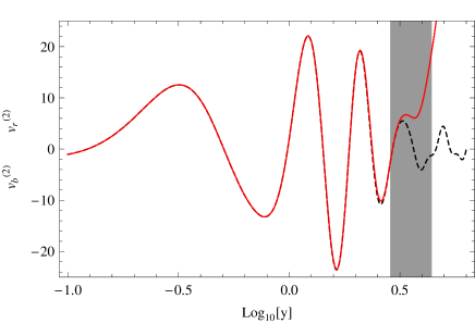
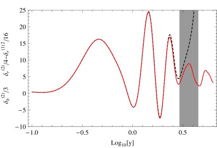
Figure 2: Top: Comparison of the baryons and photons velocity perturbation at order 2 for $k_{1}=k_{2}=10k_{\mathrm{eq}}$ and $\textbf{k}_{1}\cdot\textbf{k}_{2}=0$. It shows that $v_{\rm r}^{(2)}=v_{\rm b}^{(2)}$ with a good approximation until decoupling. Bottom: l.h.s and r.h.s of Eq. (45) for the adiabaticity condition at order 2. It can be seen that this adiabaticity condition holds until recombination, hence justifying the approximation of § III.

Fig. 1 shows the evolution of the two second order gravitational potentials. In particular, it shows that the solution is driven, as expected, toward $\Phi^{(2)}=\Psi^{(2)}$. It is to be noted that the convergence takes place before equivalence, at $y\equiv 1$, as stressed in the following. On the other hand Fig. 2 depicts the evolution of the velocities and density contrasts and shows that the photons-baryons plasma can safely be described as a single fluid, almost until the decoupling (shaded area on the figure).

III Analytical insight

Before we proceed to describing the outcome of our numerical integrations, and in order to gain some insight into the physics of this intricate system, we present some analytic descriptions of its solutions.

III.1 Heuristic argument and hypothesis

Let us first assume that $f_{\rm b}\ll 1$ so that the universe is mainly dominated by non-interacting cold dark matter and radiation components. When, in the radiation era, the CDM component is completely negligible the gravitational potential is determined by the density contrast of radiation. The latter however develops oscillations after Hubble-radius crossing while those in the CDM fluid increases. It follows that, while still formally in the radiation era ($\rho_{\rm r}>\rho_{\rm c}$), the cold dark matter component is actually driving the gravitational potential. It then acts as an external driving term in the evolution equation of radiation. In such a scenario we then expect non-linearities that develop in the CDM sector to be transferred first to the gravitational potential and then to the radiation density fluctations.

To make this heuristic argument more quantitative we will thus assume that

• we can first study the CDM-plasma system to determine the gravitational potential at second order where for simplicity the plasma is assumed to be radiation dominated;

• then study the acoustic oscillations of the baryon-photon plasma driven by the gravitational potential derived this way, both at first and second order in the perturbations.

For the sake of simplicity we will work in the tight coupling approximation. We recall that the time of decoupling is both the time at which this tight coupling regime ceases to be valid and the time at which the radiation temperature is observed.

The tight coupling approximation amounts to saying that the coupling terms $\mathcal{F}_{\rm r}$ and $\mathcal{F}_{\rm b}$ are so large that radiation and baryons behave as single fluid. It ensures that the two fluids have the same peculiar velocity ($v_{\rm r}=v_{\rm b}$) and implies that the anisotropic pressure of radiation vanishes ($\pi_{\rm r}=0$).

From Eq. (17), it implies that

$$\delta_{\rm b}=\frac{3}{4}\delta_{\rm r}\ .$$ (47)

At linear order, eliminating $\mathcal{F}_{a}$ in Eq. (18) for radiation and baryons leads for the photons-baryons plasma to the continuity equation

$$\delta_{{\rm pl}}^{\prime}+3\mathcal{H}(c^{2}_{s,{\rm pl}}-w_{{\rm pl}})\delta_{{\rm pl}}+(1+w_{{\rm pl}})(\Delta v_{{\rm pl}}-3\Psi^{\prime})=0\ ,$$ (48)

and the Euler equation

$$v_{{\rm pl}}^{\prime}+\mathcal{H}(1-3c^{2}_{s,{\rm pl}})v_{{\rm pl}}+\Phi+\frac{c^{2}_{s,{\rm pl}}}{1+w_{\rm pl}}\delta_{{\rm pl}}=0\ ,$$ (49)

where we have introduced the density contrast of the plasma $\delta_{\rm pl}=\delta\rho_{\rm pl}/\rho_{\rm pl}$ with

$$\delta\rho_{\rm pl}=\delta\rho_{\rm r}+\delta\rho_{\rm b}\ ,\quad\rho_{\rm pl}=\rho_{\rm r}+\rho_{\rm b}\ .$$ (50)

In the particular case at hand, it reduces to

$$\delta_{\rm pl}=\frac{1+R}{1+\frac{4}{3}R}\delta_{\rm r}$$

and the velocity perturbation are given by

$$v_{{\rm pl}}=v_{\rm r}=v_{\rm b}\ .$$

The equation of state and sound speed of the plasma are easily obtained from the fact that $P_{{\rm pl}}=P_{\rm r}$. They are explicitly given by

$$w_{\rm pl}=\frac{1}{3+4R}\ ,\quad c^{2}_{s,{\rm pl}}=\frac{1}{3(1+R)}\ ,$$ (51)

and are time-dependent quantities (simply because the relative contribution of the two components changes with time).

At second order, the density contrast and velocity perturbation of the plasma are given by

$$\delta^{(2)}_{\rm pl}=\frac{(1+R)\delta^{(2)}_{\rm r}-\frac{R}{4}\delta_{\rm r}^{(1)2}}{1+\frac{4}{3}R},\quad v^{(2)}_{{\rm pl}}=v^{(2)}_{\rm r}=v^{(2)}_{\rm b}\ .$$

It can be checked that the plasma follows the equation (48) and (49) but supplemented with the source terms

$$S_{c,{\rm pl}}=S_{c,a={\rm pl}}\,\qquad S_{e,{\rm pl}}=S_{e,a={\rm pl}},$$ (52)

where $S_{c,a={\rm pl}}$ and $S_{e,a={\rm pl}}$ stand for $S_{c,a}$ and $S_{e,a}$ in which we take the fluid to be the plasma, that is $\delta_{a}=\delta_{\rm pl},\,\,w_{a}=v_{\rm pl}$, etc.

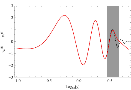
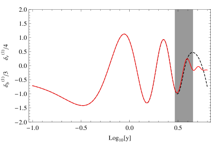
Figure 8: Left: Comparison of the baryons and photons velocity perturbation at first order for $k=10k_{\mathrm{eq}}$. It shows that $v_{\rm r}^{(1)}=v_{\rm b}^{(1)}$ with a good approximation until decoupling. Right: Comparison of $\frac{1}{4}\delta_{\rm r}^{(1)}$ and $\frac{1}{3}\delta_{\rm r}^{(1)}$. It can be seen that the adiabaticity condition holds until recombination, hence justifying the approximation of § III.

The validity of the tight coupling approximation at first and second order can be checked from our numerical integration (which indeed does not make this assumption) respectively on Fig. 2 and Fig. 8 for the second and first orders.

III.2 CDM-radiation system

III.2.1 First order

Deep in the radiation era, the gravitational potential is mainly determined by the radiation density contrast and decays on sub-Hubble scales. The contribution of matter is negligible in the Poisson equation and it follows that the potential is given by

$$\Phi(k,\eta)=3\Phi(k,\eta_{\textrm{init}})\frac{j_{1}(c_{s,{\rm r}}x)}{c_{s,{\rm r}}x},$$ (53)

where $j_{1}$ is a spherical Bessel function of order 1 and $x=k\eta$. The density contrast of radiation is given by $\delta_{\rm r}=-2\Phi$ on super-Hubble scales (see § II.4.1).

Let us now turn to the evolution of the CDM fluid during the radiation era. In terms of the variable $y$ the continuity and Euler equations lead to

$$\ddot{\delta}_{c}+\frac{2+3y}{2y(1+y)}\dot{\delta}_{c}=S_{\Phi}(y)\ ,$$ (54)

with a driving force determined by the gravitational potential

$$S_{\Phi}(y)=3\ddot{\Phi}+\left[\frac{6+9y}{2y(1+y)}\right]\dot{\Phi}-\frac{2}{1+y}\left(\frac{k}{k_{\mathrm{eq}}}\right)^{2}\Phi\ ,$$ (55)

where a dot stands for a derivative with respect to $y$. The general solution of Eq. (54) is of the form $\delta_{c}(k,\eta)=A+B\ln x+\delta_{\rm part}$ where $\delta_{\rm part}$ is a particular solution given by

$$\delta_{\rm part}=\int_{\eta_{\textrm{init}}}^{\eta}S_{\Phi}(k,\eta^{\prime})\,\eta^{\prime}\ln\left(\frac{\eta}{\eta^{\prime}}\right){\rm d}\eta^{\prime}\ ,$$

where $S_{\Phi}$ is given by Eq. (53) as long as $\delta\rho_{\rm c}\ll\delta\rho_{\rm r}$. For $y\ll 1$, the contribution of the particular solution is negligible so that $A\simeq-\frac{3}{2}\Phi(\eta_{\textrm{init}})$ and $B\simeq 0$. The solution (53) shows that $\Phi$ vary mainly when $\eta\sim k^{-1}$ so that $\delta_{\rm part}\sim A+B\ln x$. $A$ and $B$ can be obtained semi-analytically and are well approximated by $A\simeq 6$ and $B\simeq-9$ so that $\delta_{\rm c}\simeq\Phi(k,\eta_{\textrm{init}})(-4.5+9\ln x)$.

This solution is valid as long as $\delta\rho_{c}\ll\delta\rho_{r}$ in the Poisson equation. However, on sub-Hubble scales $\delta_{\rm r}$ remains constant while, as we just saw, $\delta_{c}$ grows logarithmically. Their contribution in the Poisson equation then become to be of the same order when $y\sim y_{\star}(k)$, where $y_{\star}$ is solution of $y_{\star}[-4.5+9\ln(\sqrt{2}y_{\star}k/k_{\mathrm{eq}})]\sim 6/(1-f_{{}_{\rm b}})$, where use has been made of $x=\sqrt{2}ky/k_{\mathrm{eq}}$ as long as $y\ll 1$,. The solution of this equation is depicted on Fig. 3. For most of the scales of interest, i.e. for $k\gg k_{\rm eq.}$, the contribution of the CDM in the Poisson equation is dominant before equality, i.e. $y_{\star}<1$).

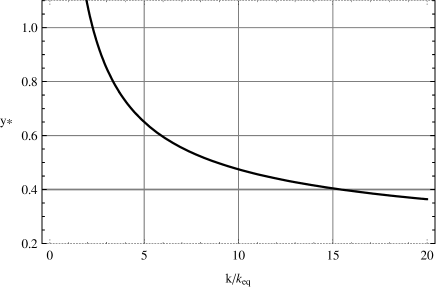
Figure 3: The time at which the contribution of cold dark matter and of radiation are comparable in the Poisson equation as a function of $k/k_{\mathrm{eq}}$. $k_{\mathrm{eq}}$ is the wave-number of the mode that becomes sub-Hubble at the time of quality. For most of the scales of interest, i.e. for $k\gg k_{\rm eq.}$, the contribution of CDM in the Poisson equation is dominant before equality, i.e. $y_{\star}<1$).

For these modes, which became sub-Hubble during the radiation era, we shall consider that CDM dominates in the Poisson equation and neglect the contribution of the radiation density perturbation, so that the Poisson equation takes the form

$$k^{2}\Phi=-\frac{3(1-f_{{}_{\rm b}})}{4y}k_{\mathrm{eq}}^{2}\delta_{\rm c}\ .$$ (56)

Neglecting the contribution of baryons, since their density contrast cannot grow because they are tightly coupled to the radiation, Eq. (54) then takes the form of the Mészáros equation Mészáros (1974)

$$\ddot{\delta}_{\rm c}+\frac{2+3y}{2y(1+y)}\dot{\delta}_{\rm c}-\frac{3}{2y(y+1)}\delta_{\rm c}=0\ .$$ (57)

Its two solutions are a growing mode

$$D_{+}(y)=y+2/3$$ (58)

and the decaying mode

$$D_{-}(y)=-2\sqrt{(1+y)}+D_{+}(y)\ln\left(\frac{\sqrt{1+y}+1}{\sqrt{1+y}-1}\right)\ .$$ (59)

III.2.2 Second order

At second order, as at first order, while deep in the radiation era the gravitational potential generated by the density contrast of radiation decays when a mode becomes sub-Hubble. At this order the gravitational potential satisfies

$$\Psi^{\prime\prime}+4\mathcal{H}\Psi^{\prime}-\frac{1}{3}\Delta\Psi = S_{r}\ ,$$ (60)

with

$$S_{r}=S_{2}-\frac{1}{3}S_{1}+\frac{1}{3}\Delta S_{3}+\mathcal{H}S_{3}^{\prime}\ ,$$

where the source terms are given by Eqs. (31-34). Up to a fast decaying solution, the general solution is

$$\Psi(\eta)=3\Psi(k,\eta_{\textrm{init}})\frac{j_{1}(c_{s,{\rm r}}x)}{c_{s,{\rm r}}x}+\int_{\eta_{\textrm{init}}}^{\eta}G_{r}(k,\eta,\eta^{\prime})S_{r}(\eta^{\prime}){\rm d}\eta^{\prime}\ ,$$ (61)

with the Green function

$$G_{r}(k,\eta,\eta^{\prime}) = -\frac{\eta^{\prime}}{c_{s,{\rm r}}^{3}x^{3}}\Big{\{}\left(c_{s,{\rm r}}^{2}xx^{\prime}+1\right)\sin\left[c_{s,{\rm r}}(x-x^{\prime})\right]$$ (62)

$$-c_{s,{\rm r}}(x-x^{\prime})\cos\left[c_{s,{\rm r}}(x-x^{\prime})\right]\Big{\}}\ .$$

On sub-Hubble scales, the leading terms in $S_{r}$ are those quadratic in the first order velocity, of the form $\propto\mathcal{H}^{2}\partial^{i}v\partial_{i}v\sim\eta^{-2}$, which behave as $\eta^{-2}$. All other terms in $S_{r}$ behave, at best, as $k^{-2}\eta^{-4}$. Using the first order solution, the second order gravitational potential asymptotically behaves as

$$\Psi^{(2)}_{S}(k,\eta) \simeq -\frac{81}{2}\mathcal{C}\frac{\Psi^{(1)}(k_{1},\eta_{\textrm{init}})\Psi^{(1)}(k_{2},\eta_{\textrm{init}})}{k^{2}\eta^{2}(1-\mu^{2})}$$ (63)

$$\times\left[1+2\left(\frac{1}{k_{1}^{2}}+\frac{1}{k_{2}^{2}}\right)\mathbf{k}_{1}\cdot\mathbf{k}_{2}+3\left(\frac{\mathbf{k}_{1}\cdot\mathbf{k}_{2}}{k_{1}k_{2}}\right)^{2}\right]$$

$$\times\left[\cos\left(c_{s,{\rm r}}k_{1}\eta\right)\cos\left(c_{s,{\rm r}}k_{2}\eta\right)-\cos\left(c_{s,{\rm r}}k\eta\right)\right.$$

$$\qquad\qquad\left.-\mu\sin\left(c_{s,{\rm r}}k_{1}\eta\right)\sin\left(c_{s,{\rm r}}k_{2}\eta\right)\right]\ ,$$

and it can be checked that this term is indeed regular in $\mu^{2}=1$. Taking the homogeneous solution into account, $\Psi^{(2)}$ decays as $(k\eta)^{-2}$ on sub-Hubble scales.

Now, the evolution of the density contrast of CDM follows, using $y$ as the time variable, the evolution equation

$$\ddot{\delta}_{c}^{(2)}+\frac{2+3y}{2y(1+y)}\dot{\delta}_{c}^{(2)}$$ (64)

$$-3\ddot{\Psi}^{(2)}-\left[\frac{6+9y}{2y(1+y)}\right]\dot{\Psi}^{(2)}+\frac{2}{1+y}\left(\frac{k}{k_{\mathrm{eq}}}\right)^{2}\Phi^{(2)}=S_{\delta_{c}}\ ,$$

where the source term is given by

$$S_{\delta_{c}}\equiv\frac{1}{k_{\mathrm{eq}}}\sqrt{\frac{2}{1+y}}\left(\dot{S}_{c}+\frac{S_{c}}{y}\right)+\frac{2}{1+y}\left(\frac{k}{k_{\mathrm{eq}}}\right)^{2}S_{e}\ .$$

As in the previous section for the first order perturbations, CDM density perturbations grow faster than those of radiation so that, for any mode $k$ that became sub-Hubble before $\eta_{\mathrm{eq}}$, there exists a time of order $y_{\star}[k]$ such that for $y>y_{\star}[k]$ the gravitational potential at second order is determined by the cold dark matter. Whereafter, even though we are still in the radiation era, we can neglect the contribution of the density perturbation of radiation so that the Poisson equation becomes

$$k^{2}\Phi^{(2)}\simeq k^{2}\Psi^{(2)}\simeq-\frac{3(1-f_{{}_{\rm b}})}{4y}k_{\mathrm{eq}}^{2}\delta^{(2)}_{c}\ .$$ (65)

In this regime, the evolution of the density contrast of CDM at second order can be derived from a second order Mészáros-like equation, in a similar way as at first order. Using Eq. (65) and the fact that the main contributions in $S_{\delta_{c}}$ in this regime come from

$$S_{c}\simeq-2\partial_{i}\left(\delta\partial^{i}v\right),\quad\partial_{i}S_{e}\simeq-2\left(\partial_{j}v\partial^{j}\partial_{i}v\right)\ ,$$ (66)

Eq. (64) takes the form

$$\ddot{\delta}_{c}^{(2)}+\frac{2+3y}{2y(1+y)}\dot{\delta}_{c}^{(2)}-\frac{3(1-f_{{}_{\rm b}})}{2y(1+y)}\delta_{c}^{(2)}=S_{M}\ ,$$ (67)

with

$$S_{M} = \mathcal{C}\Bigg{\{}\left[2\delta_{c}\ddot{\delta}_{c}+2\dot{\delta}_{c}^{2}+\frac{\delta_{c}\dot{\delta}_{c}}{y(1+y)}\right]+2\frac{\mathbf{k}_{1}\cdot\mathbf{k}_{2}}{k_{1}^{2}k_{2}^{2}}\dot{\delta}_{c}^{2}$$

$$+\left[\delta_{c}\ddot{\delta}_{c}+2\dot{\delta}_{c}^{2}+\frac{\delta_{c}\dot{\delta}_{c}}{2y(1+y)}\right]\mathbf{k}_{1}\cdot\mathbf{k}_{2}\left(\frac{1}{k_{1}^{2}}+\frac{1}{k_{2}^{2}}\right)\Bigg{\}}\,.$$

Now we shall neglect the effect of baryons, that is $f_{\rm b}$. This equation could then be called the second order Mészáros equation and describes a growth of CDM density perturbation in a regime where radiation dominates the dynamics of the background while its density perturbations are negligible in the Poisson equation.

The Green function associated to this equation is obtained to be

$$G(y,y^{\prime}) = \frac{3}{2}y^{\prime}\sqrt{1+y^{\prime}}(2+3y)(2+3y^{\prime})\times$$ (69)

$$\left[\frac{\sqrt{1+u}}{2+3u}-\frac{1}{6}\ln\frac{\sqrt{1+u}+1}{\sqrt{1+u}-1}\right]_{u=y^{\prime}}^{u=y}\ ,$$

so that the general solution of Eq. (67) is

$$\delta_{c}^{(2)}=C_{1}D_{+}(y)+C_{2}D_{-}(y)+\int_{0}^{y}G(y,y^{\prime})S_{M}(y^{\prime}){\rm d}y^{\prime}\ .$$

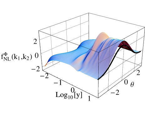
Figure 4: (solid line) The second order potential computed in the tight coupling limit as a function of time $y$ and of $\theta$, angle between the wave vectors. It is compared to its expected late time behaviour (72). It is to be noted that the convergence toward this solution is extremely rapid and takes place as soon as equality is reached, e.g. $y=1$. The results correspond to $k_{1}=6k_{\mathrm{eq}}$ and $k_{2}=12k_{\mathrm{eq}}$. The difference in the amplitude of the function is due to the fact that the baryons component has been neglected in the derivation of Eq. (72)

.

In the limit where $y\gg 1,\,y^{\prime}\gg 1$, the Green function behaves as

$$G(y,y^{\prime})\simeq\frac{2}{5}y\left[1-\left(\frac{y^{\prime}}{y}\right)^{5/2}\right],$$

and the source term as

$$S_{M}\simeq 7\mathcal{C}K(\mathbf{k}_{1},\mathbf{k}_{2})\frac{\delta(k_{1})\delta(k_{2})}{y^{2}}\ ,$$

with the Kernel

$$K(\mathbf{k}_{1},\mathbf{k}_{2})\equiv\left[\frac{5}{7}+\frac{1}{2}\mathbf{k}_{1}\cdot\mathbf{k}_{2}\left(\frac{1}{k_{1}^{2}}+\frac{1}{k_{2}^{2}}\right)+\frac{2}{7}\frac{(\mathbf{k}_{1}\cdot\mathbf{k}_{2})^{2}}{k_{1}^{2}k_{2}^{2}}\right]\ .$$ (70)

In the limit $y\gg 1$, the particular solution dominates and our solution converges toward

$$\frac{1}{2}\delta^{(2)}(k)\simeq\mathcal{C}K(\mathbf{k}_{1},\mathbf{k}_{2})\delta_{c}(k_{1})\delta_{c}(k_{2})\ ,$$ (71)

that is toward the standard result (I) describing the collapse of cold dark matter in a matter dominated era. The second order gravitational potential is then obtained from the Poisson equation

$$\frac{1}{2}\Phi^{(2)}(k,\eta)\simeq-\mathcal{C}\frac{1}{6}K(\mathbf{k}_{1},\mathbf{k}_{2})\left(\frac{k_{1}k_{2}\eta}{k}\right)^{2}\Phi(k_{1})\Phi(k_{2}),$$ (72)

up to terms of order $\mathcal{O}(f_{\rm b})$. The convergence towards the solution (72) is explicitly depicted on Fig. 4 where the behaviour of the exact (numerically integrated) second order potential as a function of time (and angle) is compared to its expected late time behaviour (72). As detailed above, this solution is a better approximation for larger wave-numbers and at large $y$ since we converge to this solution for $y>y_{\star}(k)$. On this figure it can be observed that the convergence is extremely rapid and that the full kernel structure, including its angular dependence in (72), is indeed to be observed in $\Phi^{(2)}$.

III.3 Baryons-radiation system

We now want to understand the behaviour of the baryons-photons plasma, and in particular of its acoustic oscillation, in the regime in which the gravitational potential is determined by the solutions of the previous section.

We restrict our analysis to the tight coupling regime. And since it occurs for $y<y_{\mathrm{LSS}}$, our solution will gain in accuracy when the period between CDM domination, $y=y_{\star}(k)$, and the last scattering surface, $y=y_{\mathrm{LSS}}$, is large, that is on the smallest scales.

III.3.1 First order

The computation at first order is well known Hu and Sugiyama (1996) and we review its main steps to compare to the more unexplored second order case.

In the fluid limit, the baryons and photons both obey a continuity and conservation equations (17-18) with a source term and in which the anisotropic stress of radiation can be neglected because of the tight-coupling approximation. As discussed in § III.1, in the tight coupled regime, that is for $k/\tau^{\prime}\ll 1$, it leads to the wave equation

$$\left(\frac{\delta_{\rm r}}{4}-\Psi\right)^{\prime\prime}+\frac{R^{\prime}}{1+R}\left(\frac{\delta_{\rm r}}{4}-\Psi\right)^{\prime}+k^{2}c_{s}^{2}\left(\frac{\delta_{\rm r}}{4}-\Psi\right)$$

$$\qquad\qquad\simeq\frac{-k^{2}}{3}\left[\Phi\left(1+\frac{1}{1+R}\right)\right]\ ,$$ (73)

where $R$ is defined in Eq. (13), the sound speed is given by Eq. (51). This is a wave equation with a forcing term on the r.h.s. which describes the oscillations of the plasma.

For small wavelength modes, the variation of $R$ and $\Phi$ is small compared to the period of the wave so that we can construct an adiabatic solution by resorting on a WKB approximation; see e.g. Ref. Hu and Sugiyama (1996) for details. Defining

$$\Theta_{\text{SW}}\equiv\frac{1}{4}\delta_{\rm r}+\Phi$$

and the sound horizon

$$r_{s}(\eta)\equiv\int_{0}^{\eta}\frac{1}{\sqrt{3[1+R(\eta^{\prime})]}}{\rm d}\eta^{\prime}\ ,$$

the WKB solution takes the form

$$\Theta_{SW}(k,\eta)=\frac{\left[\Theta_{SW}(0)+R\Phi\right]}{(1+R)^{1/4}}\cos[kr_{s}(\eta)]-R\Phi\ .$$ (74)

The velocity field, $v_{\rm r}=v_{\rm b}$ can then be determined from the Euler equation (49).

This solution neglects the Silk damping effect that can be described by adding terms in $k^{2}/\tau^{\prime}$ in Eq. (III.3.1) so that the solution is exponentially suppressed by a factor

$$\mathcal{D}(k,\eta)=\exp\left(-\frac{k^{2}}{k_{D}^{2}}\right)$$

where

$$k_{D}^{-2}(\eta)\sim\frac{1}{6}\int_{0}^{\eta}\frac{1}{1+R(\eta^{\prime})}\left[\frac{16}{15}+\frac{R^{2}(\eta^{\prime})}{1+R(\eta^{\prime})}\right]\frac{{\rm d}\eta^{\prime}}{\tau^{\prime}(\eta^{\prime})}\ ,$$

so that

$$\Theta_{SW}+R\Phi\propto\exp\left({-\frac{k^{2}}{k_{D}^{2}}}\right)\ ,$$ (75)

where the damping scale is of the order of $k_{D}\sim 15k_{\mathrm{eq}}$. Since $\Phi$ decreases as $(k/k_{\mathrm{eq}})^{-2}$, we conclude that for large wavenumber, $\Theta_{SW}(k,\eta)$ goes rapidly to zero.

III.3.2 Second order

The former approach can be generalised at second order, but the behaviour of $\Theta_{SW}$ will change mainly because the second order version of Eq (III.3.1) has a r.h.s. which is steadily growing in the range of interest, i.e. after $\eta_{\mathrm{eq}}$ and on large $k$.

At second order, Eq. (III.3.1) will also contain terms coming from the second order Liouville equation Pitrou (2007) of the form

$$S_{\rm pl}=\frac{1}{4}\left(S_{c,{\rm r}}^{\prime}+\frac{R^{\prime}}{1+R}S_{c,{\rm r}}\right)+\frac{k^{2}}{3}S_{e,{\rm pl}}\,.$$

This source term involves terms which are quadratic in the fluid perturbation variables ($\delta,v$) and the potentials ($\Phi,\Psi$). The former are exponentially suppressed due to Silk damping and the latter decrease as $(k/k_{\mathrm{eq}})^{-2}$. We can thus neglect this source term as long as we focus on small scales. Defining,

$$\Theta_{SW}^{(2)}\equiv\frac{\delta_{\rm r}^{(2)}}{4}+\Phi^{(2)}\ ,$$ (76)

the solution for $\Theta_{SW}^{(2)}$ will be similar to Eq. (75). When Silk damping is taken into account, $\Theta_{SW}^{(2)}+R\Phi^{(2)}$ is exponentially suppressed, exactly as at first order. The main difference with first order arises from the fact that the second order gravitational potentials are driven toward $\Psi^{(2)}\simeq\Phi^{(2)}\sim(k\eta)^{2}$ after equivalence ($y>y_{\mathrm{eq}}$) so that we expect that

$$\Theta_{SW}^{(2)}\equiv\frac{\delta_{\rm r}^{(2)}}{4}+\Phi^{(2)}\simeq-R\Psi^{(2)}\ .$$ (77)

Now, the velocity of radiation is given by

$$\left[(1+R)v_{\rm r}^{(2)}\right]^{\prime}=-\frac{\delta^{(2)}_{\rm r}}{4}-(1+R)\Phi^{(2)}\ .$$ (78)

Since $\Theta_{SW}^{(2)}+R\Phi^{(2)}$ is exponentially suppressed due to the Silk damping, we expect that the Doppler contribution is also negligible.

The equations (72) and (77) are the central results of the analytic insight of the non-linear regimes of the photons-baryons-CDM system at second order. They give the behaviour of the second order gravitational potentials at the time of decoupling together with the response of the photon-electron plasma. We also conclude that we expect $\Theta_{SW}^{(2)}=-R\Phi^{(2)}$ to dominate the CMB temperature anisotropies on small angular scales (see Appendix B for a discussion of the integrated Sachs-Wolfe contribution).

The bottom line of our analytic estimates is that on small angular scales, i.e. $k/k_{\mathrm{eq}}\gg 1$, the density perturbation of CDM starts to dominate the Poisson equation from $y_{\star}(k)$ so that from this time to decoupling we can assume that the system is split in (1) the evolution of CDM and (2) the evolution of the photons-baryons plasma which develops acoustic oscillations in the gravitational potential determined by the CDM component. Because of Silk damping, $\Theta_{SW}+R\Phi$ dies out on small scales. At first order this implies that $\Theta_{SW}^{(1)}\sim-R\Phi^{(1)}$ which is suppressed by a factor $k_{\mathrm{eq}}^{2}/k^{2}$ due to its evolution in the radiation era prior to $y_{\star}(k)$. At second order however, we still have for the same reason that $\Theta_{SW}^{(2)}\sim-R\Phi^{(2)}$ but now this term roughly grows as $(k\eta)^{2}$. Note that since $k_{D}$ is of order $15k_{\mathrm{eq}}$ and that $k_{\mathrm{eq}}$ roughly corresponds to a multipole $\ell\sim 160$, we expect our analysis to give a good description of the system for $\ell\gtrsim 2400$.

III.4 Comparison to numerics

We now turn to the description of the numerical solutions of the system described in § II.5. Its solutions will be described in the light of the analytic description we just developed.

Fig. 5 shows the result of numerical integrations for second order quantities of interest. They are compared to our approximate formula that, we recall, is expected to be valid in the tight coupling regime. It shows indeed that modes with $k>k_{\mathrm{eq}}$ relax temporarily toward the solution (77). The exact solution exhibits though large oscillations that are thought to be due to the acoustic oscillations that are present in the plasma at first order, but their average turns out to coincide with the proposed analytic formula (long dashed lines) as long as a strong coupling is ensured. The Silk damping effect is observed to play a key role to actually damping the oscillations. This effect is all the more important that $k$ is large. Note that the impact of the oscillations on the observational quantities will also be damped by the finite width of the last scattering surface. The wave-number corresponding to this width is of order of $10k_{\mathrm{eq}}$ which is smaller than the damping scale.

When the coupling becomes loose, $\log_{10}(y)$ approaching $0.6$, the numerical solution departs from the expected solution (and it converges toward 0) as the full Boltzmann hierarchy is now at play. We also depict the velocity term which can be checked to be negligible, as expected.

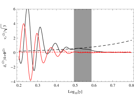
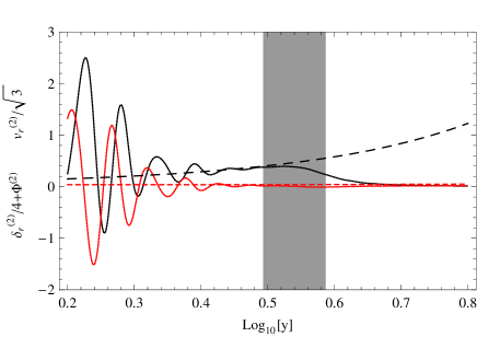
Figure 5: Behavior of $\Theta_{SW}^{(2)}$ (black) and $kv_{\rm r}^{(2)}/\sqrt{3}$ (red). The numerical integration is depicted with solid lines while the analytical estimates is plotted in dashed lines. From top to bottom, we have $k_{1}=k_{2}=30\,k_{\rm eq.}$ and $k_{1}=k_{2}=40\,k_{\rm eq.}$. The vertical grey zone represents the “surface” of last scattering.

From these set of results we can then argue that the approximate analytic solution described in (77) captures the physics of the dominant terms of the CMB anisotropies on small angular scales. Here we have explicitly checked that this form is consistent with the physics of recombination when the collision effects are taken into account. We limit though the collision effects to their first order expression. We expect nonetheless that an exact calculation, up to second order, would not significantly alter our conclusions, the collision physics playing a role only during a limited period of time. Although this is certainly desirable to do such a calculation, this is beyond the scope of this paper whose goal is to estimate the order of magnitude of the non-Gaussianity on these scales.

In the following we explore the observational consequence of such a finding on the temperature bispectrum at small scale.

IV Signature in the cosmic microwave background

IV.1 Flat sky approximation

Since our approximations hold on small angular scales, it is amply sufficient to treat the sky as flat to compute the properties of the CMB anisotropies. We thus decompose the CMB temperature anisotropies in 2D-Fourier space as

$$\Theta(\mathbf{n})=\int\frac{{\rm d}^{2}\mathbf{l}}{2\pi}\Theta(\mathbf{l})\,\hbox{e}^{\textrm{i}\mathbf{l}\cdot\mathbf{n}}\ ,$$ (79)

so that

$$\Theta(\mathbf{l})=\int\frac{{\rm d}^{2}\mathbf{n}}{2\pi}\Theta(\mathbf{n})\,\hbox{e}^{\textrm{-i}\mathbf{l}\cdot\mathbf{n}}\ .$$ (80)

On the other hand $\Theta(\mathbf{n})$ can be expanded in Fourier modes as

$$\Theta(\mathbf{n})=\int\frac{{\rm d}\mathbf{k}}{(2\pi)^{3/2}}\bar{\Theta}(\mathbf{k},\eta_{\mathrm{LSS}})\hbox{e}^{\textrm{i}(k_{r}\eta_{\mathrm{LSS}}+D_{\mathrm{LSS}}\mathbf{k_{\perp}}\cdot\mathbf{n})}\ ,$$ (81)

where $D_{\mathrm{LSS}}$ is the angular distance of the last scattering surface given by $D_{\mathrm{LSS}}=\int_{y_{LSS}}^{y_{0}}1/(H[u]u){\rm d}u$. $\mathbf{k}_{\perp}$ is the projection of $\mathbf{k}$ on the sky, ı.e. $\mathbf{k}=k_{r}\mathbf{e}+\mathbf{k_{\perp}}$ where $\mathbf{e}$ is the direction of the (flat) sky.

In Eq. (81) we refer to $\bar{\Theta}(\textbf{k},\eta_{\mathrm{LSS}})$ as

$$\bar{\Theta}(\textbf{k},\eta_{\mathrm{LSS}})=\int{\rm d}\eta\Theta(\mathbf{k},\eta)v(\eta,\eta_{\mathrm{LSS}})\ ,$$ (82)

considering the observed CMB anisotropies as a superposition of spheres of temperature anisotropy weighted by the visibility function $v(\eta,\eta_{\mathrm{LSS}})$ which peaks at $\eta_{\mathrm{LSS}}$. The angular power spectrum is nothing but the two dimensional power spectrum of $\Theta(\mathbf{l})$,

$$\langle\Theta(\mathbf{l})\Theta(\mathbf{l}^{\prime})\rangle=\delta^{(2)}(\mathbf{l}+\mathbf{l}^{\prime})C_{l}\ .$$ (83)

We now need to determine $\Theta(\textbf{k},\eta)$ in terms of the perturbation variables. The CMB temperature anisotropies are usually split as an intrinsic Sachs-Wolfe effect, a Doppler effect and an integrated Sachs-Wolfe contribution. As discussed in Appendix B the integrated Sachs-Wolfe contribution is expected to be negligible on the scales of interest in our study.

At first order, the Fourier component of temperature anisotropy for a mode $\mathbf{k}$, in a direction $\mathbf{e}$ emitted at a comoving distance $\eta_{0}-\eta$ is dominated by the Sachs-Wolfe and Doppler terms,

$$\Theta^{(1)}(\mathbf{k},\eta) = \Theta^{(1)}_{SW}(\mathbf{k},\eta)+\Theta^{(1)}_{\rm Dop}(\mathbf{k},\eta)$$ (84)

$$\equiv g^{(1)}(\mathbf{k},\eta)\Phi^{(1)}_{k}(0)\ .$$

The Sachs-Wolfe term is related to the perturbation variables by

$$\Theta^{(1)}_{SW}(\mathbf{k},\eta)=\frac{\delta^{(1)}_{r}}{4}(\mathbf{k},\eta)+\Phi^{(1)}(\mathbf{k},\eta)\ ,$$ (85)

while the Doppler term is given $\Theta_{\text{Dop}}\equiv-v\mathbf{k}.\mathbf{e}$ so that

$$\Theta^{(1)}_{\rm Dop}(\mathbf{k},\eta) = \textrm{i}k_{r}v^{(1)}_{r}(\mathbf{k},\eta)\ ,$$ (86)

with $k_{r}=\textbf{k}\cdot\mathbf{e}$. Using Eq.(81), we deduce thus that

$$\Theta^{(1)}(\mathbf{l}) = \frac{1}{\sqrt{2\pi}D_{\mathrm{LSS}}^{2}}\int{\rm d}k_{r}\hat{g}^{(1)}(\mathbf{k})\hbox{e}^{\textrm{i}k_{r}\eta_{\mathrm{LSS}}}\ ,$$ (87)

with

$$\hat{g}^{(1)}(\mathbf{k})=\int{\rm d}\eta v(\eta)g^{(1)}(\mathbf{k},\eta)\Phi^{(1)}(\textbf{k},0)\$$ (88)

and where $\textbf{k}_{\perp}=\mathbf{l}/D_{\mathrm{LSS}}$. Using the definition of the initial power spectrum $\langle\Phi(\textbf{k},0)\Phi(\textbf{k}^{\prime},0)\rangle=\delta^{(3)}(\mathbf{k}+\textbf{k}^{\prime})P(k)$, we finally get that $C_{l}$ is given by

$$C_{l}\simeq\frac{1}{2\pi D_{\mathrm{LSS}}^{2}}\int{\rm d}k_{r}P\left(\sqrt{k_{r}^{2}+\frac{l^{2}}{D_{\mathrm{LSS}}^{2}}}\right)\left|\hat{g}^{(1)}(\mathbf{k})\right|^{2}.$$ (89)

This reproduces the main features of the CMB angular power spectrum, as checked on Fig. 9.

At second order, and for the scales of interest ($k\gg k_{eq}$ and $k>k_{D}$), we stress again that the knowledge of the exact expression of the terms quadratic in the first order variables in the second order Sachs-Wolfe effect are not needed since they are suppressed because of the Silk damping or because of the decaying of the potential during the radiation era. The analysis of § III.3.2 shows that the Doppler term is much smaller than the intrinsic Sachs Wolfe term of Eq. (77). Thus, the main contribution to the second order temperature anisotropy is well approximated by

$$\Theta^{(2)}(\textbf{k},\eta) \simeq \Theta^{(2)}_{SW}(\textbf{k},\eta)\ ,$$ (90)

$$\simeq \frac{\delta^{(2)}_{\rm r}(\textbf{k},\eta)}{4}+\Phi^{(2)}(\textbf{k},\eta)\simeq-R\Phi^{(2)}\ .$$

We deduce that

$$\Theta^{(2)}(\mathbf{l}) = \frac{1}{\sqrt{2\pi}D_{\mathrm{LSS}}^{2}}\int{\rm d}k_{r}\hat{g}^{(2)}(\mathbf{k})\hbox{e}^{\textrm{i}k_{r}\eta_{\mathrm{LSS}}}\ ,$$ (91)

with

$$\hat{g}^{(2)}(\mathbf{k})=\int{\rm d}\eta\,v(\eta)\,\Theta^{(2)}(\textbf{k},\eta).$$ (92)

It can be rewritten in terms of the initial first order gravitational potential as

$$\hat{g}^{(2)}(\mathbf{k})=2\mathcal{C}\ f_{{}_{\rm NL}}^{(\Theta)}(\textbf{k}_{1},\textbf{k}_{2})\Phi^{(1)}(\textbf{k}_{1},0)\Phi^{(1)}(\textbf{k}_{2},0)\ ,$$ (93)

hence defining $f_{{}_{\rm NL}}^{(\Theta)}$.

IV.2 Bispectrum

In the flat sky approximation, the reduced bispectrum $b_{l_{1}l_{2}l_{3}}$ is defined from the 3-point function as

$$\langle\Theta({\bf l}_{1})\Theta({\bf l}_{2})\Theta({\bf l}_{3})\rangle=(2\pi)^{-1}\delta^{(2)}({\bf l}_{1}+{\bf l}_{2}+{\bf l}_{3})b_{l_{1}l_{2}l_{3}}\ ;$$ (94)

see e.g. Ref. Komatsu (2002). With the previous definitions, it can be expressed as

$$b_{l_{1}l_{2}l_{3}} = \frac{1}{2\pi D_{\mathrm{LSS}}^{4}}\int{\rm d}k_{r1}{\rm d}k_{r2}\left[f_{{}_{\rm NL}}^{(\Theta)}(-\mathbf{k}_{1},-\mathbf{k}_{2})\hat{g}^{(1)}(\mathbf{k}_{1})\hat{g}^{(1)}(\mathbf{k}_{2})P\left(\sqrt{k_{r1}^{2}+\frac{\textbf{k}_{\perp 1}^{2}}{D_{\mathrm{LSS}}^{2}}}\right)P\left(\sqrt{k_{r2}^{2}+\frac{\textbf{k}_{\perp 2}^{2}}{D_{\mathrm{LSS}}^{2}}}\right)\right]$$ (95)

$$\qquad\qquad+\left(\mathbf{l_{1}}\rightarrow\mathbf{l_{2}}\rightarrow\mathbf{l_{3}}\rightarrow\mathbf{l_{1}}\right)+\left(\mathbf{l_{1}}\rightarrow\mathbf{l_{3}}\rightarrow\mathbf{l_{2}}\rightarrow\mathbf{l_{1}}\right)\ .$$

IV.3 Numerical computation

In order to perform the previous integrals, we need to specify the initial power spectrum. We assume that the power spectrum is scale invariant and we normalize it using the results of WMAP, that is

$$P(k)=2\pi^{2}\frac{25}{9}A_{s}^{2}\left(\frac{k_{\mathrm{eq}}}{k}\right)^{3}\frac{1}{k_{\mathrm{eq}}^{3}}$$ (96)

with

$$A_{S}^{2}=3.33\times 10^{-10}\ .$$ (97)

We then compute the bispectrum of an equilateral configuration for which all momentums are equals; $l_{1}=l_{2}=l_{3}$. The only free parameter for such configuration is the norm $l$ of the three vectors.

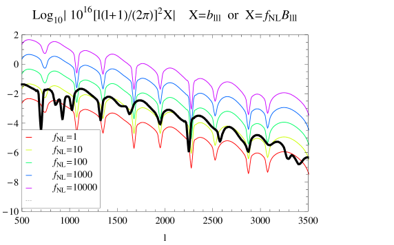
Figure 6: Black: the bispectrum for the equilateral configuration computed in the flat sky limit. The thin colored lines represents the bispectrum that would be obtained by assuming a constant initial $f_{{}_{\rm NL}}^{\Phi}$ and a linear transfer function, that is neglecting the non-linear dynamics. From bottom to top we have plotted $f_{{}_{\rm NL}}^{\Phi}=1,10,100,1000,10000$.

The result is depicted on Fig. 6 and is compared to the bispectrum one would obtain from a initial constant $f_{{}_{\rm NL}}^{\Phi}$ assuming a linear transfer function. It appears that on scales that range from $l=1000$ to $l=3000$ the bispectrum resembles that of an effective constant primordial $f_{{}_{\rm NL}}^{\Phi}$ of order 25.

The order of magnitude of the amplitude of the bispectrum can be understood from the following rule of thumb for modes larger than $k_{D}$. According to our analysis, considering the equilateral configuration where $k_{1}=k_{2}=k$, the second order temperature anisotropy on the last scattering surface is of order

$$\frac{1}{2}\Theta^{(2)}(\textbf{k},\eta_{\mathrm{LSS}}) \simeq -\frac{1}{2}R_{\mathrm{LSS}}\Phi^{(2)}(\textbf{k},\eta_{\mathrm{LSS}})$$

$$\simeq -R_{\mathrm{LSS}}\frac{2y_{\mathrm{LSS}}}{3}\frac{k^{2}}{k_{\mathrm{eq}}^{2}}\left[\Phi^{(1)}(k,0){\cal T}_{\theta}^{(1)}(k)\right]^{2}$$

where we have assumed that, on average, the Kernel $K(\mathbf{k}_{1},\mathbf{k}_{2})$ is of order unity. Now, assuming a constant primordial $f_{{}_{\rm NL}}$ evolved with the linear transfer function, the second order temperature anisotropy would roughly be of order

$$\frac{1}{2}\Theta^{(2)}(\textbf{k},\eta_{\mathrm{LSS}})\simeq-R_{\mathrm{LSS}}f_{\text{NL}}\left[\Phi^{(1)}(k,0)\right]^{2}{\cal T}_{\theta}^{(1)}(k)$$ (98)

since, for these modes, the integral on the visibility function keeps only the average of the Sachs-Wolfe contribution. The ratio of the contribution of the non-linear dynamics compared to a primordial non-Gaussianity is

$$\frac{2}{3}\frac{y_{\mathrm{LSS}}}{f_{{}_{\rm NL}}}\left(\frac{k}{k_{\mathrm{eq}}}\right)^{2}{\cal T}_{\theta}^{(1)}(k)\ .$$ (99)

Since for large modes the gravitational potential has been decaying as $(k\eta)^{-2}$ in the radiation dominated era, and growing logarithmically when the potential started to be determined by the cold dark matter component(see the analysis of section III.2.1), we deduce that the first order transfer function is typically given by

$${\cal T}_{\theta}^{(1)}(k)\simeq A(k)\left(\frac{k_{\mathrm{eq}}}{k}\right)^{2}\ ,$$ (100)

where $A(k)$ is a steadily growing function. At the Silk damping scale we find numerically $A(k_{D})\simeq 10$. We thus conclude that in the bispectrum, the evolution for $l\simeq k_{D}D_{\mathrm{LSS}}\simeq 2400$ is equivalent to a primordial

$$f_{{}_{\rm NL}}\simeq\frac{2}{3}y_{\mathrm{LSS}}A(k_{D})\simeq 25$$

evolved linearly. This estimates of the order of magnitude is in complete agreement with Fig. 6 where it can be read that for multipole ranging from 2000 to 3000 the amplitude of the bispectrum is comparable with the one that would be obtained from a constant $f_{{}_{\rm NL}}$ ranging between 10 and 50.

There is no guarantee however that for arbitrary geometries the shape dependence of the temperature bispectrum would be that of a constant $f_{{}_{\rm NL}}$. It is rather determined by the kernel shape of the form (77).

V Conclusion

This article investigates the non-Gaussianity that arises in the CMB temperature anisotropies due to the post-inflationary non-linear dynamics during the radiation and matter dominated era. More specifically it aims at identifying the leading mechanisms and leading terms that determine the shape of the CMB bispectrum on small angular scales.

The driving idea that we have pursued throughout the paper is that at small angular scales the second order CMB anisotropies trace the second order gravitational potential as it is shaped by the CDM component during its sub-Hubble evolution. To give support to this picture, we have developed both analytical insights into the joint evolution of the density potentials and the temperature fluctuations and numerical tools.

We have thus solved numerically the joint evolution equations of the cosmic fluids up to second order. We have been able to check that at the time of decoupling, the second order potential indeed traces its expected shape. This conclusion is summarised and illustrated on Fig. 4. At this stage, and as long as one restricts these results to the tight coupling regime, no approximations have been made. The accuracy with which the $k$-dependence of the matter dominated mode coupling kernel, i.e. Eq. (I), is recovered is truly remarkable. We stress that this is due to the fact that for the physics at work at small scales, i.e. $k/k_{\mathrm{eq}}\gg 1$, the density perturbations of the CDM component start to dominate the Poisson equation much before equality. This implies that the non-linearities developed by the CDM can be transferred very efficiently to the gravitational potential even before the beginning of the matter era.

Determining exactly how this mode coupling kernel is actually transferred to the source term of the CMB anisotropies relies on further numerical integrations through the recombination era. At this stage, the only approximation we make concerns the Compton scattering collision term entering the Boltzmann equation for radiation at second order. We did not use its full second order expression but we argue that it can be reduced to its formal first order form, namely to Eq. (30). Such an assumption is clearly valid in the tight coupling regime. Actually this is the only term appearing in the collision term in the baryons rest-frame as long as tight coupling at first order is efficient. We then argue that when the coupling drops, Silk damping effects effectively suppress all other contributions.

This leads to the behaviour depicted on Fig. 5 for the main source term of the temperature anisotropies. In particular $\Theta_{SW}^{(2)}$, the monopole of the second order source term, is found to be attracted toward a non-vanishing and non-oscillatory term, $-R\Phi^{(2)}$, where we recall that $R$ is the baryon to radiation ratio, while the dipole contribution, and thus the Doppler effect, vanishes. As a result the main contribution to the CMB temperature anisotropies at second order is found to be directly proportional to the second order gravitational potential. It has to be noted that the efficiency with which the second order term converges to this form is considerably accelerated by the Silk damping effects which efficiently suppress the oscillatory parts of the solution. This results are clearly illustrated on Fig. 5. We argued from order of magnitude arguments that, because the damping scale is typically of order $15k_{\mathrm{eq}}$, our description shall be valid for $l\gtrsim 2400$. This observation is the basis of the main result of this paper. Actually,as Fig. 6 tends to show, it seems that this description may be valid at lower multipoles.

Finally we explore the consequence on the CMB bispectrum. For obvious reasons we use the small angle approximation to perform the numerical integrations. The bispectrum for equilateral configurations is illustrated on Fig. 6. We show that for these configurations, its amplitude corresponds to what a primordial non-Gaussian potential of $f_{{}_{\rm NL}}^{\Phi}$ of order 25 would have given (also for an equilateral configuration). As shown in the text, this number can easily be recovered from back-of-the-envelop calculations. The first lesson that can be drawn from this result is that it gives a signal larger than what a model with a primordial $f_{{}_{\rm NL}}$ of order unity would give! The second lesson is that the $l$-dependence of the bispectrum is expected to be different from the one induced by primordial mode couplings. It is expected to have a specific shape as encoded in the CDM kernel expression.

In conclusion, this work offers a breakthrough insight into the physics of CMB in the non-linear regime and on small angular scales. It identifies what is, as we argued, the main small scale contribution of the bispectrum, hence filling the gap with the standard results that have been obtained in the weakly non-linear regime of gravitational clustering of dark matter. We did not check this result against a (yet non-existing) full second order Boltzmann code, and this is probably desirable, but we argue that, given the amplitude of the effects, all other contributions will be subdominant. With such a large signal, detection of this bispectrum should be easily within reach of future CMB experiments!

Acknowledgements: We thank J. Martin-Garcia for his help in using the tensorial perturbation calculus package xPert Martin-Garcia (2006) that was used to derive the second order expressions of this paper. We also thank G. Faye, Y. Mellier, S. Prunet, D. Spergel and N. Aghanim for many discussions.

Appendix A Description of radiation

To describe the evolution of radiation, we use the first moments of the Boltzmann hierarchy (see e.g. Refs. Hu and White (1997)) including polarisation. The hierarchy reads

$$\Theta_{\ell}^{\prime} = k\left[\frac{\ell}{2\ell-1}\Theta_{\ell-1}-\frac{\ell+1}{2\ell+3}\Theta_{\ell+1}\right]$$ (101)

$$-\tau^{\prime}\left[\Theta_{\ell}-\delta_{\ell 2}\frac{1}{10}\left(\Theta_{2}-\sqrt{6}E_{2}\right)\right]$$

$$E_{\ell}^{\prime} = k\left[\frac{\sqrt{\ell^{2}-4}}{2\ell-1}E_{\ell-1}-\frac{\sqrt{(\ell+1)^{2}-4}}{2\ell+3}E_{\ell+1}\right]$$ (102)

$$-\tau^{\prime}\left[E_{\ell}+\delta_{\ell 2}\sqrt{6}\left(\Theta_{2}-\sqrt{6}E_{2}\right)\right]$$

where the first moments are related to the fluid variables by

$$\Theta_{0}=\frac{1}{4}\delta_{\rm r}\ ,\quad\Theta_{1}=-kv_{\rm r}\ ,\quad\Theta_{2}=\frac{5}{12}k^{2}\pi_{\rm r}\ .$$

The Boltzmann hierarchy is infinite and we truncated it after the multipole $\ell=8$, when computing the first order and after $\ell=3$ when computing the second order. In order to cut the hierarchy without numeric reflection Ma and Bertschinger (1995), we use the free-streaming solution of this hierarchy, and use it to express in the last equation the multipole $\ell+1$ in function of the multipoles for $\ell$ and $\ell-1$. Explicitly, the closure relation reads

$$\Theta_{\ell+1} = \frac{2\ell+3}{k\eta}\Theta_{\ell}-\frac{2\ell+3}{2\ell-1}\Theta_{\ell-1}$$ (103)

$$E_{\ell+1} = \frac{(2\ell+3)\sqrt{\ell+1}}{k\eta\sqrt{\ell-1}}E_{\ell}-\frac{(2\ell+3)\sqrt{(\ell+3)(\ell+2)}}{(2\ell-1)\sqrt{(\ell-1)(\ell-2)}}E_{\ell-1}\,.$$

Appendix B The Integrated Sachs-Wolfe effect contribution to the small scale bispectrum

At linear order, the contribution of the integrated Sachs-Wolfe effect on small scales is usually small because the time dependence of the potential vanishes in the matter dominated era. This is no more the case at second order. It is thus legitimate to investigate the impact of the time dependence of the second order gravitational potential on the amplitude of the bispectrum.

At linear order the expression of the temperature anisotropies is

$$\Theta^{(1)}(\mathbf{l})=\frac{\sqrt{2\pi}}{D_{\mathrm{LSS}}^{2}}\int\hat{g}(\mathbf{k})\,{\rm d}k_{r}$$ (104)

while at second order an extra source term should be included. It is formally given by

$$\Theta^{(2)}_{\rm ISW}(\mathbf{l})=\int_{0}^{\eta_{\mathrm{LSS}}}{\rm d}\eta\frac{{\rm d}}{{\rm d}\eta}\left\{\Psi^{(2)}[\textbf{x}(\eta),\eta]+\Phi^{(2)}[\textbf{x}(\eta),\eta]\right\}\,\,\,\,$$ (105)

assuming instantaneous recombination at $\eta=\eta_{\mathrm{LSS}}$. To estimate the magnitude of this effect, we assume that $\Psi^{(2)}=\Phi^{(2)}$ and that the time dependence is the one otained in Eq. (72),

$$\Psi^{(2)}(\eta)=\frac{\eta^{2}}{\eta_{\mathrm{LSS}}^{2}}K_{NL}(\textbf{k}_{1},\textbf{k}_{2},\eta_{\mathrm{LSS}})\ ,$$ (106)

where the time dependence has been explicited. Obviously, expression (105) gives an extra term contributing to the bispectrum. Consistently with our former analysis, let us evaluate this contribution in the small angle approximation. This leads to

$$b_{\textbf{l}_{1}\textbf{l}_{2}\textbf{l}_{3}}^{\rm ISW} = 4\int_{-\infty}^{\infty}{\rm d}k_{r_{1}}{\rm d}k_{r_{2}}\,P(k_{1})\,P(k_{2})\,K_{NL}(\textbf{k}_{1},\textbf{k}_{2},\eta_{\mathrm{LSS}})$$ (107)

$$\times\int_{0}^{\eta_{\mathrm{LSS}}}{\rm d}\eta_{1}v(\eta_{1})\,{\rm d}\eta_{2}v(\eta_{2})\,\frac{{\rm d}\eta\ \eta}{\eta_{\mathrm{LSS}}^{2}}g(\textbf{k}_{1},\eta_{1})g(\textbf{k}_{2},\eta_{2})$$

$$\times\exp\left[{\rm i}k_{r_{1}}\eta_{\mathrm{LSS}}+{\rm i}k_{r_{2}}\eta_{\mathrm{LSS}}\right]+{\hbox{sym.}}$$

that has to be compared with  Eq.(95). The integral over $\eta$ can then be performed to give

$$b_{\textbf{l}_{1}\textbf{l}_{2}\textbf{l}_{3}}^{\rm ISW} \approx 4\int_{-\infty}^{\infty}{\rm d}k_{r_{1}}{\rm d}k_{r_{2}}\,P(k_{1})\,P(k_{2})\,K_{NL}(\textbf{k}_{1},\textbf{k}_{2},\eta_{\mathrm{LSS}})$$ (108)

$$\times\int_{0}^{\eta_{\mathrm{LSS}}}{\rm d}\eta_{1}v(\eta_{1})\,{\rm d}\eta_{2}v(\eta_{2})\,g(\textbf{k}_{1},\eta_{1})g(\textbf{k}_{2},\eta_{2})$$

$$\times w(k_{r_{1}}+k_{r_{2}},\eta_{\mathrm{LSS}})+{\hbox{sym.}}$$

with

$$w(k,\eta_{\mathrm{LSS}})=\frac{1-{\rm i}k\eta_{\mathrm{LSS}}-\exp({\rm i}k\eta_{\mathrm{LSS}})}{k^{2}\,\eta_{\mathrm{LSS}}^{2}}\ .$$ (109)

If one examines the UV convergence properties of this expression (for the integrals over $k_{r}$), it appears that the integral over $k_{r_{1}}+k_{r_{2}}$ converges at a scale given by the inverse of $\eta_{\mathrm{LSS}}$, e.g.

$$\int_{-\infty}^{\infty}{\rm d}k\ w(k,\eta_{\mathrm{LSS}})=\frac{\pi}{\eta_{\mathrm{LSS}}}\ ,$$ (110)

due to the oscillatory behaviour of $w$, whereas the integral over $k_{r_{1}}-k_{r_{2}}$ converges because of the power spectrum shape and therefore at a scale which is of the order of $l_{1}/\eta_{\mathrm{LSS}}$ or $l_{2}/\eta_{\mathrm{LSS}}$ (whichever is smaller).

Thus if the power spectrum is approximated by a power law,

$$P_{\Phi}(k)\sim k^{n_{s}-4}\ ,$$ (111)

where the spectral index $n_{s}$ varies a priori from $1$ (at very large scale) to $-3$ at very small ones – it is a priori of the order of say $-2$ at the scales of interest – then the integral over $k_{r_{1}}-k_{r_{2}}$ leads to the factor,

$$\int_{-\infty}^{\infty}{\rm d}k\,P_{\Phi}^{2}(\sqrt{k_{r}^{2}+l^{2}/\eta_{\mathrm{LSS}}^{2}}) =$$ (112)

$$\frac{l^{2(n_{s}-3)-1}\sqrt{\pi}\eta_{\mathrm{LSS}}^{7-2n_{s}}\Gamma\left(\frac{7}{2}-n_{s}\right)}{\Gamma(4-n_{s})}$$

that is $63\pi/256\ (\eta_{\mathrm{LSS}}/l)^{11}$ for $n_{s}=-2$.

This is to be compared with the amplitude of the intrinsic effects we have computed. The latter differs in Eq. (95) because of the absence of filtering function $w$. The amplitude of the bispectrum is then roughly given by,

$$b_{\textbf{l}_{1}\textbf{l}_{2}\textbf{l}_{3}}^{\rm LSS} \approx 2R\,\int_{-\infty}^{\infty}{\rm d}k_{r_{1}}{\rm d}k_{r_{2}}\,P_{\Phi}(k_{1})\,P_{\Phi}(k_{2})$$ (113)

$$\quad\times K_{NL}(\textbf{k}_{1},\textbf{k}_{2},\eta_{\mathrm{LSS}})$$

so that its amplitude is dominated by the square of

$$\int_{-\infty}^{\infty}{\rm d}k_{r}P_{\Phi}(\sqrt{k_{r}^{2}+l^{2}/\eta_{\mathrm{LSS}}^{2}}) =$$ (114)

$$\frac{\eta_{\mathrm{LSS}}^{3-n_{s}}l^{2\left(\frac{n_{s}}{2}-1\right)-1}\sqrt{\pi}\Gamma\left(\frac{3}{2}-\frac{n_{s}}{2}\right)}{\Gamma\left(2-\frac{n_{s}}{2}\right)}\ ,$$

which is equal to $(3\pi/8)^{2}\ (\eta_{\mathrm{LSS}}/l)^{10}$ for $n_{s}=-2$. The ratio of the two contributions scales then as $1/(Rl)$ in favor of the intrinsic effect.

Appendix C Check of the numerical integration

We report in this appendix the results of the first order numerical integration. We first report in Figs. 7 and 8 the evolution of the perturbed quantities where it can be seen that for $y>y_{\star}(k)$ the gravitational potential tends to be determined by the cold dark matter density perturbation. We also report the angular power spectrum obtained from the flat sky approximation using the expression (89). The linear dynamics is then used to calculate the bispectrum arising from a constant primordial $f_{{}_{\rm NL}}$ evolved linearly. It can be checked that the form obtained on Fig. 9 is completely consistent with the literature (see e.g. Ref. Komatsu (2002)).

Figure 7: From top to bottom, left to right: evolution of the Bardeen potential, $\Phi$, and the density contrast $\delta$ for respectively radiation, baryons and cold dark matter. The solid line corresponds to $k=10k_{\mathrm{eq}}$ and the dashed line corresponds to $k=20k_{\mathrm{eq}}$.

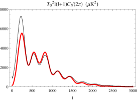
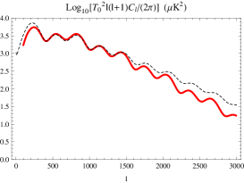
Figure 9: Left: in solid red line, the angular power spectrum using our code and the flat sky approximation (which does not includes the late ISW). The black dashed line represents the spectrum obtained using CAMB, which also takes into account the late ISW, but no reionisation. Middle: The precision on small scale depends highly on the computation of the visibility function. On small scales, our transfer function is approximately $30\%$ smaller than the one predicted by CAMB and is thus a good approximation. Right: the bispectrum obtained from a primordial constant $f_{{}_{\rm NL}}=100$ evolved linearly.

References

- Komatsu et al. (2008) E. Komatsu et al. (WMAP) (2008), eprint 0803.0547.
- Bardeen (1980) J. M. Bardeen, Phys. Rev. D 22, 1882 (1980).
- Mukhanov et al. (1992) V. F. Mukhanov, H. A. Feldman, and R. H. Brandenberger, Phys. Rept. 215, 203 (1992).
- Sasaki and Stewart (1996) M. Sasaki and E. D. Stewart, Progress of Theoretical Physics 95, 71 (1996), eprint astro-ph/9507001.
- Uzan and Peter (2005) J.-P. Uzan and P. Peter, Cosmologie primordiale (Belin, 2005).
- Bernardeau (2007) F. Bernardeau, Cosmologie, des fondements théoriques aux observations (Editions du CNRS et EDP Sciences, 2007).
- Gangui and Mollerach (1996) A. Gangui and S. Mollerach, Phys. Rev. D54, 4750 (1996), eprint astro-ph/9601069.
- Durrer et al. (2000) R. Durrer, R. Juszkiewicz, M. Kunz, and J.-P. Uzan, Phys. Rev. D62, 021301 (2000), eprint astro-ph/0005087.
- Perivolaropoulos (1993) L. Perivolaropoulos, Phys. Rev. D48, 1530 (1993), eprint hep-ph/9212228.
- Pen et al. (1994) U.-L. Pen, D. N. Spergel, and N. Turok, Phys. Rev. D 49, 692 (1994).
- Maldacena (2003) J. Maldacena, Journal of High Energy Physics 5, 13 (2003), eprint astro-ph/0210603.
- Komatsu (2002) E. Komatsu, ArXiv Astrophysics e-prints (2002), eprint astro-ph/0206039.
- Bartolo et al. (2002) N. Bartolo, S. Matarrese, and A. Riotto, Phys. Rev. D 65, 103505 (2002), eprint hep-ph/0112261.
- Bernardeau and Uzan (2002) F. Bernardeau and J.-P. Uzan, Phys. Rev. D 66, 103506 (2002), eprint hep-ph/0207295.
- Bernardeau and Uzan (2003) F. Bernardeau and J.-P. Uzan, Phys. Rev. D 67, 121301 (2003), eprint astro-ph/0209330.
- Lyth and Wands (2002) D. H. Lyth and D. Wands, Physics Letters B 524, 5 (2002), eprint hep-ph/0110002.
- Bartolo et al. (2004a) N. Bartolo, E. Komatsu, S. Matarrese, and A. Riotto, Phys. Rept. 402, 103 (2004a), eprint astro-ph/0406398.
- Bartolo et al. (2004b) N. Bartolo, S. Matarrese, and A. Riotto, Journal of High Energy Physics 4, 6 (2004b), eprint arXiv:astro-ph/0308088.
- Bernardeau et al. (2006) F. Bernardeau, T. Brunier, and J.-P. Uzan, AIP Conf. Proc. 861, 821 (2006), eprint astro-ph/0604200.
- Bernardeau and Uzan (2004) F. Bernardeau and J.-P. Uzan, Phys. Rev. D 70, 043533 (2004), eprint astro-ph/0311421.
- Alishahiha et al. (2004) M. Alishahiha, E. Silverstein, and D. Tong, Phys. Rev. D 70, 123505 (2004), eprint hep-th/0404084.
- Weinberg (2005) S. Weinberg, Phys. Rev. D 72, 043514 (2005), eprint hep-th/0506236.
- Peebles (1980) P. J. E. Peebles, The large-scale structure of the universe (Research supported by the National Science Foundation. Princeton, N.J., Princeton University Press, 1980. 435 p., 1980).
- Bernardeau et al. (2002) F. Bernardeau, S. Colombi, E. Gaztañaga, and R. Scoccimarro, Phys. Rept. 367, 1 (2002).
- Scoccimarro et al. (2001) R. Scoccimarro, H. A. Feldman, J. N. Fry, and J. A. Frieman, Astrophys. J. 546, 652 (2001), eprint arXiv:astro-ph/0004087.
- Osano et al. (2007) B. Osano, C. Pitrou, P. Dunsby, J.-P. Uzan, and C. Clarkson, JCAP 0704, 003 (2007), eprint gr-qc/0612108.
- Lu et al. (2008) T. H.-C. Lu, K. Ananda, and C. Clarkson, Phys. Rev. D77, 043523 (2008), eprint 0709.1619.
- Baumann et al. (2007) D. Baumann, P. J. Steinhardt, K. Takahashi, and K. Ichiki, Phys. Rev. D76, 084019 (2007), eprint hep-th/0703290.
- Pitrou (2007) C. Pitrou, Class. Quant. Grav. 24, 6127 (2007), eprint 0706.4383.
- Nakamura (2007) K. Nakamura, Prog. Theor. Phys. 117, 17 (2007), eprint gr-qc/0605108.
- Bruni et al. (1997) M. Bruni, S. Matarrese, S. Mollerach, and S. Sonego, Class. Quant. Grav. 14, 2585 (1997), eprint gr-qc/9609040.
- Uzan (1998) J.-P. Uzan, Class. Quant. Grav. 15, 1063 (1998), eprint gr-qc/9801108.
- Bartolo et al. (2006) N. Bartolo, S. Matarrese, and A. Riotto, Journal of Cosmology and Astro-Particle Physics 6, 24 (2006), eprint astro-ph/0604416.
- Pitrou (2008) C. Pitrou, (2008), eprint 0809.3036.
- Dodelson and Jubas (1995) S. Dodelson and J. M. Jubas, Astrophys. J. 439, 503 (1995), eprint astro-ph/9308019.
- Malik and Wands (2004) K. A. Malik and D. Wands, Classical and Quantum Gravity 21, L65 (2004), eprint arXiv:astro-ph/0307055.
- Vernizzi (2005) F. Vernizzi, Phys. Rev. D 71, 061301 (2005), eprint arXiv:astro-ph/0411463.
- Mészáros (1974) P. Mészáros, Astron. Astrophys. 37, 225 (1974).
- Hu and Sugiyama (1996) W. Hu and N. Sugiyama, Astrophys. J. 471, 542 (1996), eprint arXiv:astro-ph/9510117.
- Martin-Garcia (2006) J. Martin-Garcia, “xAct and xPert” (2006), eprint http://metric.iem.csic.es/Martin-Garcia/xAct/.
- Bernardeau et al. (2004) F. Bernardeau, T. Brunier, and J.-P. Uzan, Phys. Rev. D 69, 063520 (2004), eprint astro-ph/0311422.
- Maartens et al. (1999) R. Maartens, T. Gebbie, and G. F. R. Ellis, Phys. Rev. D59, 083506 (1999), eprint astro-ph/9808163.
- Bartolo et al. (2007) N. Bartolo, S. Matarrese, and A. Riotto, Journal of Cosmology and Astro-Particle Physics 1, 19 (2007), eprint astro-ph/0610110.
- Hu and White (1997) W. Hu and M. J. White, Phys. Rev. D56, 596 (1997), eprint astro-ph/9702170.
- Ma and Bertschinger (1995) C.-P. Ma and E. Bertschinger, Astrophys. J. 455, 7 (1995), eprint astro-ph/9506072.
- Komatsu (2002) E. Komatsu (2002), eprint astro-ph/0206039.