How edge states are destroyed in disordered mesoscopic samples?

Abstract

We report theoretical investigations on how edge states are destroyed in disordered mesoscopic samples by calculating a “phase diagram” in terms of energy versus disorder strength $(E,W)$, and magnetic field versus disorder strength $(B,W)$, in the integer quantum Hall regime. It is found that as the disorder strength $W$ increases, edge states are destroyed one by one if transmission eigen-channels are used to characterize the edge states. Near the insulating regime, transmission eigen-channels are closed one by one in the same order as edges states are destroyed. To identify those edge states which have survived disorder, we introduce a generalized current density that can be calculated and visualized.

When a two-dimensional mesoscopic sample is subjected to external magnetic field, peculiar electronic states — edge states, may be established at the boundaries of the sampleHelperin82 ; buttiker88 . Classically, Lorentz force pushes electrons toward the sample boundary and electron trajectories become skipping orbits. Edge states can be considered as the quantum version of skipping orbitsbuttiker88 . Importantly, edge states in mesoscopic samples provide necessary density of states (DOS) between the Landau levels, integer quantum Hall effect (IQHE) can therefore occur in the clean sample limitbuttiker88 . In contrast, for infinitely large samples, a degree of disorder in the sample appears necessary which provides DOS in between Landau levels to stablize the Fermi energy for IQHEprange-book . Nevertheless, increasing disorder will eventually destroy IQHE and how does this happen has been an important issue attracting numerous studies.

Here we address the disorder issue for mesoscopic samples, namely how edge states are destroyed by disorder in the IQHE regime and, at a fixed filling factor $\nu>1$, are edge states destroyed all at once or one by one. These important questions provide insight to the IQHE phase diagram for mesoscopic samples, and may shed light to similar problems in samples of infinite size. We address these questions by extensive calculations on a mesoscopic graphene system and a square lattice model (see inset of Fig.1a) to map out a “phase diagram” of edge states in the presence of disorder. Here the “phases” in the “phase diagram” denote quantum states and no phase transitions are implied between these states. We use transmission eigen-channels to characterize edge states (see below), and we found that they are destroyed one by one. At large enough disorder, the system becomes an insulator and transmission eigen-channels are closed one by one in the same order as the edge states are destroyed.

We begin by discussing our definition of edge states as well as the way to visualize them. In transport theory, for each incoming channel of a semi-infinite lead $\alpha$ whose wave function is $|W_{\alpha,m}>$ where $m=1,2,\cdots N$ denotes one of the $N$ channels, one solves a scattering problem. $|W_{\alpha,m}>$ is an eigen-channel of lead-$\alpha$ but not the entire device. To find the eigen-channels of the entire device, we diagonalizebuttiker1 the transmission matrix ${\cal T}$ by a unitary transformation $U$, for a two probe device having scattering matrix $S_{RL}$, ${\cal T}=S^{\dagger}_{RL}S_{RL}$. Mathematically, this means acting $U$ on the incoming channels $|W_{\alpha,m}>$ (which is a column vector with N components) to obtain a new set of orthogonal incoming modes $|{\bar{W}}_{\alpha m}>=\sum_{n}|W_{\alpha,n}>U_{nm}$. Once done, $|{\bar{W}}_{\alpha,m}>$ is an eigen-state of the entire device (leads plus scattering region). In other words, if an incoming electron comes at state $|{\bar{W}}_{\alpha,m}>$, it will traverse the entire device without mixing with any other eigen-state $|{\bar{W}}_{\alpha,m^{\prime}}>$. This way, the resulting transmission matrix ${\bar{\cal T}}=U^{\dagger}{\cal T}U$ is diagonal. In the presence of a strong magnetic field $B$, it is therefore natural to identify $|{\bar{W}}_{\alpha m}(B)>$ as edge states because they are the eigen-states or eigen-channels of the entire device sample. How to visualize edge states in the IQHE regime? This may be achieved by plotting the current density in real space. The subtle issues of current density in IQHE has been discussed in Ref.Hirai, . In our work where there are disorder in the sample, the eigen-channels provide a convenient way to define a generalized current density for each channel — since the eigen-channels do not mix. Clearly, the total transport current is obtained by integrating current density along any cross-section perpendicular to the transport direction.

The total transmission coefficient is obtained from the $N\times N$ Hermitian transmission matrix ${\cal T}=\{t_{ij}\}$. Applying an unitary transformation $U$buttiker1 , we obtain ${\bar{\cal T}}=U^{\dagger}{\cal T}U=\{t_{i}\delta_{ij}\}$, which is diagonal with elements $t_{i}$. The transmission coefficient $t_{i}$ of eigen-channel $i$ is a linear combination of $t_{ij}$. Using conventional current density ${\bf J}_{ii}=(ie\hbar/2m)(\psi_{i}\nabla\psi_{i}^{*}-\psi^{*}_{i}\nabla\psi_{i})-(e^{2}/m){\bf A}|\psi_{i}|^{2}$ with $i=1,2,\cdots N$, it is easy to show $(e^{2}/h)~{}t_{ii}=\int{\bf J}_{ii}\cdot d{\bf s}$ in the linear bias regime, where $t_{ii}$ is the diagonal element of matrix ${\cal T}$. In order to find an eigen-current density ${\bf J}_{i}$ such that

$$\frac{e^{2}}{h}~{}t_{i}=\int{\bf J}_{i}\cdot d{\bf s}\ ,$$ (1)

we define a generalized complex current density ${\bf J}_{ij}$ so that $(e^{2}/h)~{}t_{ij}=\int{\bf J}_{ij}\cdot d{\bf s}$. The unitary transformation on the incoming wave function $|W_{\alpha,m}>$ suggests the following definition:

$${\bf J}_{ij}=\frac{ie\hbar}{2m}(\psi_{j}\nabla\psi_{i}^{*}-\psi^{*}_{i}\nabla\psi_{j})-\frac{e^{2}}{m}{\bf A}\psi_{j}\psi^{*}_{i}$$ (2)

where $\psi_{i}$ is the wave function in the scattering region due to the incoming state $|W_{\alpha,i}>$. From this definition, we can prove the relationship $(e^{2}/h)~{}t_{ij}=\int{\bf J}_{ij}\cdot d{\bf s}$, as follows. It is not difficult to show that the following ${\bf J}_{i}$ satisfies Eq.(1): ${\bf J}_{i}=(ie\hbar/2m)({\bar{\psi}}_{i}\nabla{\bar{\psi}}_{i}^{*}-{\bar{\psi}}^{*}_{i}\nabla{\bar{\psi}}_{i})-(e^{2}/m){\bf A}|{\bar{\psi}}_{i}|^{2}$ where ${\bar{\psi}}_{i}=\sum_{j}\psi_{j}U_{ji}$. Using this ${\bf J}_{i}$, Eq.(1) becomes

$$\frac{e^{2}}{h}~{}t_{i}=\int\sum_{jk}U_{ji}U^{*}_{ki}{\bf J}_{kj}\cdot d{\bf s}\ .$$ (3)

Denoting ${\cal J}_{G}$ the generalized current density matrix with matrix elements ${\bf J}_{ij}$, Eq.(3) is equivalent to

$$\frac{e^{2}}{h}~{}{\bar{\cal T}}=U^{\dagger}\int{\cal J}_{G}\cdot d{\bf s}U~{}~{}{\rm or}~{}~{}\frac{e^{2}}{h}~{}{\cal T}=\int{\cal J}_{G}\cdot d{\bf s}\ .$$ (4)

We have also confirmed Eq.(4) numerically using specific examples including that shown in the inset of Fig.1a. Therefore, to obtain eigen-current density matrix, we first diagonalize the transmission matrix ${\cal T}$ to find the unitary matrix $U$; we then calculate the generalized current density ${\cal J}_{G}$ according to Eq.(2). The eigen-current density matrix is finally obtained by ${\cal J}_{\rm eigen}=U^{\dagger}{\cal J}_{G}U$ and plotted for visualization.

Can eigen-channels be measured experimentally? To answer this question, as an example let’s consider a two-probe device having two eigen-channels or two edge states in the presence of magnetic field. Assume one can perform two experiments: (i) measurement of conductance and (ii) measurement of shot noise. Clearly, conductance is given by $G=\frac{e^{2}}{h}(t_{1}+t_{2})$. The shot noise is given bybuttiker1 $S=\frac{e^{2}}{h}[t_{1}(1-t_{1})+t_{2}(1-t_{2})]$. From these $t_{1}$ and $t_{2}$ can be determined. In the case of three eigen-channels, one needs to experimentally measure an additional quantityreulet , for instance the third cumulant of current $Y=<\Delta{\hat{I}(t_{1})}\Delta{\hat{I}(t_{2})}\Delta{\hat{I}(t_{3})}>$. In the linear regime, $Y=(e^{2}/h)\sum_{i}t_{i}(1-t_{i})(1-2t_{i})$beenakker . Hence by measuring $G$, $S$, and $Y$, one can determine $t_{1,2,3}$. Therefore, the transmission eigen-channels are physical quantities measurable experimentally.

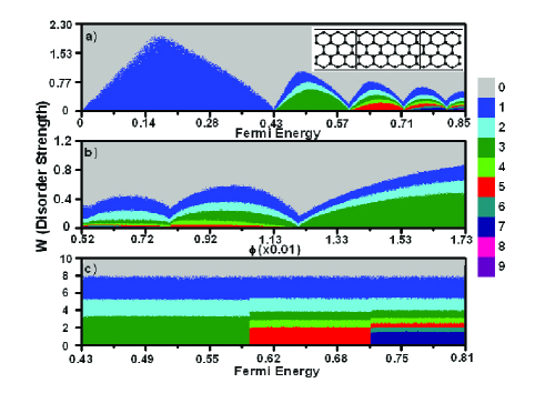
Figure 1: (color online) (a,b) are “Phase diagram” of edge states of graphene for energies near the Fermi level (Dirac electrons): (a) in the $(E,W)$ plane; (b) in the $(B,W)$ plane. (c) The order of closing of eigen-channels at large disorder. Color coding are for number of eigen-channels.

Having prepared analytical tools, we now present numerical calculations on how the edge states are destroyed by increasing degrees of disorder. In the tight-binding representation, the Hamiltonian of 2D honeycomb lattice of graphene can be written as:

$$H = \sum_{i}{\epsilon_{i}c^{\dagger}_{i}c_{i}}-t\sum_{<ij>}{e^{i{2\pi}{\phi}_{ij}}}c^{\dagger}_{i}c_{j}$$ (5)

where $c^{\dagger}_{i}$ ($c_{i}$) is the creation (annihilation) operator for an electron on site ${i}$. The first term in $H$ is the on-site single particle energy where diagonal disorder is introduced by drawing $\epsilon_{i}$ randomly from a uniform distribution in the interval $[-W/2,W/2]$ where $W$ measures the disorder strength. The second term in $H$ is due to nearest neighbor hopping that includes the effect of a magnetic field. Here the phase ${\phi_{ij}=\int{\bf A}{\cdot}d{l}/\phi_{0}}$ and $\phi_{0}=h/e$ is the flux quanta. We fix gauge so that ${\bf A}=(By,0,0)$; and current flows in the x-direction. Transmission coefficient is given by $T={\rm Tr}[{\cal T}]$ where the transmission matrix ${\cal T}$ is obtained from ${\cal T}=\Gamma_{R}G^{r}\Gamma_{L}G^{a}$ with $G^{r,a}$ being the retarded and advanced Green functions of the disordered scattering region. Quantities $\Gamma_{\alpha}$ ($\alpha=L,R$) are the line width functions obtained by calculating self-energies $\Sigma^{r}$ due to the semi-infinite leadslopez84 . The numerical data are mainly obtained from systems with ${32\times}56$ sites. In the calculations, energy and disorder strength are measured in unit of coupling strength $t$.

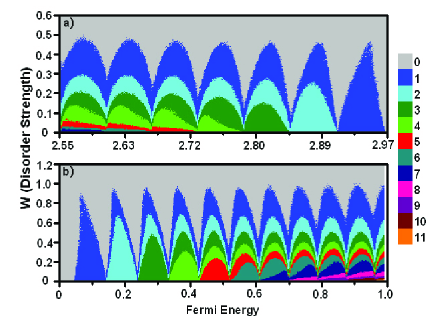
Figure 2: (color online) Phase diagram of edge states in $(E,W)$ plane for: (a) hole-like charge carriers in graphene; (b) electrons in a square lattice. The main difference between the two phase diagrams is due to opposite charges of hole and electron.

Numerically, an edge state is identified if transmission coefficient of an eigen-channel is $T\geq 0.999$; if $T\leq 0.001$, the eigen-channel is said to be closed. In addition, an edge state is said to be “destroyed” by disorder and becomes a regular eigen-channel if its transmission $T$ drops to below $0.999$. Fig.1a plots the phase diagram of edge states of graphene in the $(E,W)$ plane with $\phi=0.0173$ and energy range $[0,0.85]$ where band dispersion is linear (Dirac electrons). A mesh of $600\times 480$ points are scanned in $(E,W)$ plane and up to 200 disorder configurations are averaged at each point. Several observations are in order. First, the edge states are destroyed one by one as $W$ is increased. For instance, at $E=0.5$ the $\nu=3$ edge state is destroyed when $W=0.5$. Very importantly, we emphasize that at this disorder, there are still three transmission eigen-channels although only two are edge states and the third being a regular eigen-channel having $T<0.999$. In other words, the third eigen-channel is still there to participate transport although it is no longer an edge state. Increasing disorder to $W=0.7$, the $\nu=2$ edge state is destroyed; finally when $W=1$, all three edge states are destroyed. We note that edge states would be destroyed all at once if we had used the usual transmission coefficient for each channel $t_{ii}$ to characterize the edge states. Second, upon further increasing $W$, an insulating state is reached where all eigen-channels are closed. The order of channel closing is also one by one, in the same order as how edge states are destroyed. This is shown in Fig.1c. For instance, at $E=0.5$ there are three eigen-channels to start with, and at large disorder $W=3.1$, one of them is closed leaving only two regular eigen-channels. Third, the edge states are easily destroyed at the subband edges while at the subband center they are most robust against disorder. This is because the energy of Landau levels is located at the subband edge. In the presence of disorder, the Landau level is broadened with a finite widthHelperin82 . Hence the edge state that is close to one Landau level can easily relax toward it. Forth, it is more difficult to destroy an edge state at smaller energies. For Dirac electrons, the density of states is proportional to $\sqrt{E}$ so that the level spacing of lower Landau levels is larger than the upper ones. For electrons with smaller energy it is farther away from nearby Landau level than electrons with larger energy. Hence a larger disorder is needed to relax the electrons to the nearby Landau level. Finally, Fig.1b plots a “phase diagram” of edge states in the $(B,W)$ plane for Dirac electrons. Once again, the edge states are destroyed one by one, similar to the phase diagram in the $(E,W)$ plane.

Fig.2a depicts the “phase diagram” of edge states of graphene in $(E,W)$ plane for higher energies in the range $E=[2.545,2.97]$, where hole-like behavior occurs and band dispersion is non-linear (non-Dirac electrons). Again, edge states are destroyed one by one. While the “phase diagram” topology is similar to that for Dirac electrons (Fig.1), here the band dispersion is quadratic with equal energy spacing between the Landau levels. Due to this reason, the values of $W$ that are needed to destroy the last edge state at different subband centers are almost the same. We have also calculated the “phase diagram” of edge states of a square lattice in the $(E,W)$ plane using the same numerical method, results are shown in Fig.2b which are rather similar Fig.2a. In particular, it is more difficult to destroy edge states at low filling factor $\nu$, consistent with the result of Ref.sheng, .

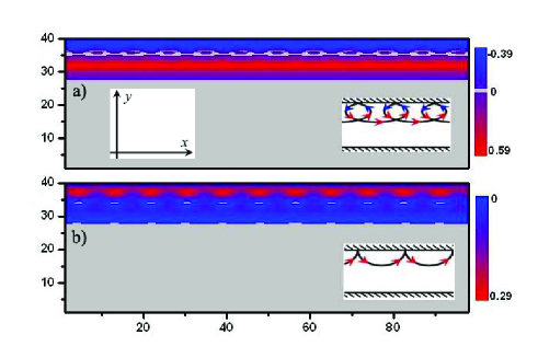
Figure 3: (color online) Current density of two edge states flowing from left to right along x-direction, for a square lattice of $100\times 40$ sites in the absence of disorder. Here $E=0.4$ and $\phi=0.052$. Note that the color scale is different for the two panels. Insets: classical skipping orbits.

Next, we examine the nature of those edge states that have survived disorder by calculating current density from Eqs.(2) and (4) and plotting it along the propagating direction (x-direction). Fig.3 shows the current density of two edge states in the absence of disorder for the square lattice model. Edge states are clearly seen. Since the two transmission eigen-channels have different longitudinal energies or effective velocities along the propagating direction, it gives two different transmission patterns that correspond to two different skipping orbits of classical trajectorybeenakker1 . In Fig.3a, current flows in the negative direction (blue region) near the sample boundary and in the positive direction (red region) away from it. There is a region between these opposite flows where the current density is very small. The classical trajectory of an electron under Lorentz force is depicted in the inset, showing a nearly completed circular motion before colliding with the sample boundary. There is an one-to-one correspondence between the classical and quantum motion: near the sample boundary the flow is from right to left, while it flows opposite away from the boundary. Similar one-to-one correspondence is also seen in Fig.3b. For the same square lattice model, Fig.4 plots the current density of two eigen-channels for a particular disorder configuration $W=1$ where the eigen transmission coefficients are $T_{1}=0.9999$ and $T_{2}=0.3385$, respectively. In the numerical calculation, we have confirmed that the integral of ${\bf J}_{i}$ over any cross-section area along the propagating direction gives the same value that is equal to $(e^{2}/h)t_{i}$. From Fig.4a, it is obvious that $T_{1}=0.9999$ is an edge state that survived this degree of disorder. Compare to Fig.3, the pattern of current density with disorder scattering is clearly different. For the eigen-channel with $T_{2}=0.3385$, it is clearly a non-edge state (Fig.3b): there is a circulating patten with large current density in the middle of the scattering region, caused by the disorder scattering. Finally, we have also calculated current density for edge states in disordered graphene, and similar behaviors are observed as that of Fig.4.

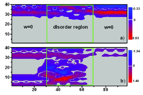
Figure 4: (color online) Current density along x-direction for the square lattice model as that of Fig.3, with disorder strength $W=1$, energy $E=0.4$ and magnetic field $\phi=0.052$. (a) For an edge state that has survived disorder; (b) edge state that has been destroyed by disorder.

In summary, we have investigated the nature of edge states in disordered mesoscopic samples in the IQHE regime. Our results show that edge states are destroyed one by one as disorder strength is increased. In the insulating regime, all transmission eigen-channels are closed and the closing is also one by one in the same order as the edge states were destroyed. For graphene and the square lattice model, the “phase diagrams” have similar topology but with some differences due to band dispersions. We have introduced a quantity which is the generalized current density, using it the current density of each eigen-channel can be calculated in the presence of disorder, giving us a vivid physical picture on how edge states are destroyed. Since transmission coefficients of individual eigen-channels for mesoscopic samples can be determined experimentally in the IQHE regime — as we discussed in the paper, our conclusions on how edge states are destroyed by disorder should be testable experimentally.

We note in passing that how to generalize our results to the large sample limit is an interesting problem requiring further investigation. In particular, based on the picture of Khmelnitskiikhmel and Laughlinlaughlin , a global phase diagram of quantum Hall effect in the $(B,W)$ plane was proposed by Kivelsonet.alkivelson for large samples which attracted considerable attention both theoreticallyref1 ; sheng and experimentallyexp1 . According to it, an integer quantum Hall state with a fixed filling factor $\nu$ will float up in energy as the disorder strength increaseskhmel ; laughlin . In the context of mesoscopic sample, this idea would mean the following. Consider Fermi level $E=E_{f}$, at the mesoscopic sample boundary there are, say, $\nu$ edge states whose eigen-values cut this energy $E_{f}$. The “float up” idea means that when disorder is increased, the energies of edge states increase to higher values, i.e. they float up. Hence, at large enough disorder there will only be $\nu-1$ edge states cutting $E_{f}$. This way, the system undergoes a series of transitions between $\nu$ to $\nu-1$ states etc.. Our results presented above, however, indicate that for mesoscopic samples edge states do not float up by disorder, they are destroyed to become regular transmission eigen-channels which participate transport.

References

- (1) B.I. Helperin, Phys. Rev. B 25, 2185 (1982).
- (2) M. Büttiker, Phys. Rev. B 38, 9375 (1988).
- (3) See, for example, articles in The Quantum Hall Effect, Eds. R.E. Prange and S.M. Girvin (Springer-Verlag, New York, 1987).
- (4) M. Buttiker, Phys. Rev. B 46, 12485 (1992).
- (5) S. Komiyama and H. Hirai, Phys. Rev. B 54, 2067 (1996).
- (6) B. Reulet et al, Phys. Rev. Lett. 91, 196601 (2003).
- (7) M. Kindermann, Yu. V. Nazarov, and C.W.J. Beenakker, Phys. Rev. Lett. 90, 246805 (2003).
- (8) M.P. López-Sancho, J.M. López-Sancho, and J. Rubio, J. Phys. F 14 1205 (1984).
- (9) D.N. Sheng and Z.Y. Weng, Phys. Rev. Lett. 78, 318 (1997).
- (10) C.W.J. Beenakker and H. van Houten, Solid State Physics 44, 1 (1991).
- (11) D.E. Khmelnitskii, Phys. Lett. A, 106, 182 (1984).
- (12) R.B. Laughlin, Phys. Rev. Lett. 52, 2304 (1984).
- (13) S. Kivelson, D.H. Lee, and S.C. Zhang, Phys. Rev. B 46, 2223(1992).
- (14) D.Z. Liu, X.C. Xie, and Q. Niu, Phys. Rev. Lett. 76, 975 (1996); Th. Koschny et. al, Phys. Rev. Lett. 86, 3863 (2001); H. Song et.al, Phys. Rev. B 76, 132202 (2007).
- (15) J. Glozman et.al, Phys. Rev. Lett. 74, 594 (1995); T. Okamoto et.al, Phys. Rev. B 52, 11109 (1995); S.V. Kravchenko et.al, Phys. Rev. Lett. 75, 910 (1995); S.H. Song et.al, Phys. Rev. Lett. 78, 2200 (1997); C.H. Lee et.al, Phys. Rev. B 58, 10629 (1998); M. Hilke et.al, Phys. Rev. B 62, 6940 (2000).