Matrix representation of the stationary measure
for the multispecies TASEP

Abstract

In this work we construct the stationary measure of the $N$ species totally asymmetric simple exclusion process in a matrix product formulation. We make the connection between the matrix product formulation and the queueing theory picture of Ferrari and Martin. In particular, in the standard representation, the matrices act on the space of queue lengths. For $N>2$ the matrices in fact become tensor products of elements of quadratic algebras. This enables us to give a purely algebraic proof of the stationary measure which we present for $N=3$.

Keywords Totally asymmetric simple exclusion process, multi-species systems, Stationary states, matrix representation

PACS 05.70.Fh 02.50.Ey 64.60.-i

1 Introduction

Models of diffusing particles with hard core interactions were first considered in the mathematical literature [1] and the name exclusion process was first coined by Spitzer [2]. In the totally asymmetric simple exclusion process (TASEP) particles jump only to the right on a one-dimensional lattice but cannot occupy the same site. Mathematical achievements include categorising the stationary measures for the process on ${\mathbb{Z}}$ and many results are summarised in the books by Liggett [3, 4].

Since the early 1990s the TASEP has been of considerable interest within the physics community as a prototypical model of nonequilibrium behaviour where, in the steady state, a current of particles is supported. In particular the model has been studied on the ring ${\mathbb{Z}}_{L}$ and also on a lattice of length $L$ with open boundary conditions where particles enter at the left boundary and leave at the right boundary. Notable achievements have been the use of the Bethe ansatz to determine spectral properties of the transition rate matrix [5, 6, 7, 8] and the determination of the stationary state in the open boundary case within a matrix product formulation [9].

A generalisation of the TASEP is to the case of several species of particle. In the two-species exclusion process containing first-class particles and second-class particles [12] both first and second-class particles hop to the right with rate 1. However if the site to the right of a first-class particle is occupied by a second-class particle the first and second-class particle exchange places with rate 1. Thus a second-class particle behaves as a hole from the point of view of a first-class particle but behaves as a particle from the point of view of a hole. The introduction of such a second class particle is a useful tool to study the microscopic structure of shocks [10, 11, 12]. Besides, the second-class particle problem arises naturally from coupling two TASEPs with different densities of particles [13]: the excess particles in the system with higher density acquire the dynamics of second-class particles. The stationary state of a system containing second and first-class particles has been obtained using the matrix product formulation by Derrida et al. [12]. Based on this work, Ferrari, Fontes and Kohayakawa [14] introduced a probabilistic construction of the measure. Angel [15] improved this construction providing a combinatorial description of the stationary state. In [16, 17], Ferrari and Martin showed that Angel’s work could be interpreted as a queueing system and they generalized it to the ${N}$ species case, for arbitrary ${N}$.

In the physics literature, the exclusion process with ${N}$ species of particles was considered by Mallick, Mallick and Rajewsky [18] and studied for the case ${N}=3$. This model, which we refer to as the ${N}$-TASEP, is defined by having site variables $\tau_{i}$ which may take values $0,1\ldots,N$ where ${N}$ is the number of species. (Note that one could alternatively consider the state $\tau_{i}=0$ (a hole) as a species which would imply a total of ${N}+1$ species; we choose instead to use the more common convention.) The dynamics is defined as follows: each bond between neighbouring lattice sites has a bell which rings with rate 1. When the bell at bond $i,i+1$ rings the site variables at $i$ and $i+1$ are exchanged provided $\tau_{i+1}=0,\tau_{i}>0$ or $\tau_{i+1}>\tau_{i}\geq 1$. This is equivalent to the following exchanges occurring with rate 1

$$K\ 0\to 0\ K \qquad\mbox{for}\quad{N}\geq K\geq 1$$ (1)

$$K\ J\to J\ K \qquad\mbox{for}\quad{N}\geq J>K\geq 1\;.$$ (2)

The construction of Ferrari and Martin [16, 17] couples ${N}$ realizations of the TASEP in a special way, called the ${N}$-line process. To the ${N}$ configurations in the ${N}$-line system one associates a configuration of the ${N}$-TASEP. Furthermore, each dynamical event of the ${N}$-line process corresponds precisely to a dynamical event in the ${N}$-TASEP. The steady state measure of the ${N}$-line system is just a uniform distribution of particles. This implies that one may sample the ${N}$-TASEP configurations with their stationary state probability by a two step procedure: (a) uniformly sampling a configuration of the ${N}$-line system of particles and (b) finding the associated configuration of the ${N}$-TASEP.

Our aim in this work is to invert this construction to obtain direct expressions for the steady state probabilities which generalise those already obtained for the two species case [12] and the three species case [18]. In doing so we shall see how the matrix product formulation generalises into a tensor product.

The paper is structured as follows. In section 2 we review the known results on the stationary measure of the 2-TASEP and show how the matrix product representation [12] is related to the queueing representation [17]. In Section 3 we consider the ${N}$-TASEP and deduce a procedure for computing the stationary state probabilities. In section 4 we construct a matrix product representation of the 3-TASEP stationary measure. In section 5 we show how matrix product representations of the ${N}$-TASEP may be obtained recursively and we conclude in section 6.

2 Two Species TASEP

In this section, we review the known solution of the two species TASEP. We also illustrate the equivalence between the matrix product solution of Derrida et al., the construction of Angel and the queueing process interpretation of Ferrari and Martin.

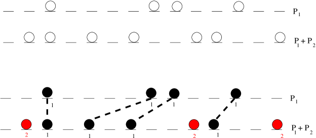
Figure 1: Graphical representation of the construction for two species.

2.1 Construction of Angel that generates the Stationary State

We begin by considering the construction of Angel for the two species TASEP on the ring ${\mathbb{Z}}_{L}$. (Note that we often use a different notation to [15] in order to avoid a clash with some standard notation from the matrix product formulation.) The construction is to consider a two-line configuration of particles (see Figure 1). On line 1 there are $P_{1}$ particles distributed randomly (with at most one particle per site) and on line 2 there are $P_{1}+P_{2}$ particles distributed randomly. Working from right to left we associate to each particle in line 1, the nearest particle, at the same site or to the left, in line 2 that has not been associated to another particle. The associated particles in line 2 are then labelled 1 and the remaining $P_{2}$ unassociated particles are labelled 2. The empty sites of line 2 are labelled 0 thus each site of line 2 is labelled 0, 1 or 2. In this way a configuration of the two species TASEP containing $P_{1}$ first-class and $P_{2}$ second-class particles has been generated through the construction. Since we consider periodic boundary conditions, the site at which we begin this procedure (chosen as the furthest site to the right in Figure 1) does not affect the two species TASEP configuration that is generated, but the particular particle in line 2 associated to a given particle in line 1 may depend on the initial starting point; for instance, if in Figure 1 one starts with the third particle from the right in line 1, then it would be associated to the fourth particle from the right in line 2, while the second particle from the right in line 1 would be associated to the fifth particle from the right in line 2. As noted in the introduction, uniformly sampling the 2-line configurations generates 2-TASEP configurations according to their stationary measure.

Angel showed that by uniformly sampling the two-line configurations, the configurations of the two-species TASEP, which we denote ${\cal C}$, are sampled with the following probabilities.

$${\rm P}({\cal C})=\frac{\prod_{j=1}^{P_{2}}\omega(B_{j})}{Z(L,P_{1},P_{2})}$$ (3)

Here $\omega(B_{j})$ is the weight of the binary string $B_{j}$ of 0,1 separating the second-class particles indexed by $j$ and $j+1$ (here $j\in{\mathbb{Z}}_{P_{2}}$ indexes the second class particles). The normalization

$$Z(L,P_{1},P_{2})={{L}\choose{P_{1}}}{{L}\choose{P_{1}+P_{2}}}$$ (4)

just counts the number of possible 2-line configurations. Note that the form of the measure (3) implies a factorization of the stationary state about the positions of the second-class particles. The reason for the factorisation is, as can be seen from Figure 1, that all 2-line configurations associated with a given 2-TASEP configuration must have the following properties: consider a site $i$, such that there is a particle labelled 2 at $i$ in line 2, then $i$ must be empty on line 1; moreover, no particle in line 1 to the right of $i$ can be associated to a particle in line 2 to the left of $i$. This factorization property, which appeared in the matrix product formulation of Derrida et al [12], was used in the construction of the stationary weights by [14].

The weights $\omega(B)$ are given by the following algorithm which we shall refer to as the pushing procedure: given the binary string $B$, one enumerates the number of strings which can be obtained from it by pushing the 1s to the right, in addition to the original string. For example from the string $110$ one obtains $110$, $101$, $011$. Thus $\omega(110)=3$. Similarly, one can obtain from $1010$ the strings $1010$, $0110$, $1001$, $0101$, $0011$. Thus $\omega(1010)=5$.

The measure given by (3) is stationary under the dynamics of the 2 species TASEP [12, 14, 15, 19]. Two key properties of this measure are i) the factorisation of the probabilities of the 2-TASEP configurations about the position of the second class particles ii) the weights $\omega(B)$ are given by the pushing procedure described above.

2.2 Matrix Product Solution of Derrida et al.

The matrix product formulation has been used to write down the stationary probabilities of various interacting particle models, thus allowing models to be solved through the explicit computation of physical quantities of interest such as currents, density profiles, correlation functions. It was first used to solve the TASEP on a lattice of length $L$ with open boundary conditions [9]. It has been extended to the 2-TASEP on the ring ${\mathbb{Z}}_{L}$ [12], partially asymmetric processes and more general reaction-diffusion systems (for a review see [20]). In this matrix product formulation properties of the stationary measure manifest themselves in algebraic relations amongst the matrices involved. Some of these relations have been classified as quadratic algebras [21].

It is important to note that the measure (3), along with the calculation of the weights $\omega(B)$, is equivalent to that first obtained within the matrix product approach, as we now show. We recall that we use the variable $\tau_{i}=0,1,2$ which implies that site $i$ is empty, contains a first-class particle or contains a second-class particle, respectively. Let us denote by ${\cal C}=(\tau_{1},\dots,\tau_{L})$, a configuration of the system. In the matrix product formulation [12] it has been proved that the stationary measure may be written as

$${\rm P}({\cal C})=Z^{-1}W({\cal C})\;,$$ (5)

where the weight of the configuration is given by

$$W({\cal C})=\mbox{Tr}\left[\prod_{i=1}^{L}X_{\tau_{i}}\right]$$ (6)

and Tr means the trace of the product of matrices $X_{\tau_{i}}$. The normalization $Z=Z(L,P_{1},P_{2})$ is chosen so that the sum of all the probabilities is equal to 1. The matrices $X_{\tau_{i}}$ are given by

$$X_{0}=E\;,\quad X_{1}=D\;,\quad X_{2}=A\;,$$ (7)

that is: if the site is empty we write a matrix $E$; if the site contains a first-class particle we write a matrix $D$; if the site contains a second-class particle we write a matrix $A$.

The matrices $D,E,A$ obey the algebraic rules

$$DE = D+E$$ (8)

$$DA = A$$ (9)

$$AE = A\;.$$ (10)

The only remaining condition to satisfy is that representations of $E$,$D$,$A$ may be found which give well-defined values for the traces appearing in (5). This may be achieved as follows. Let $|n\rangle$ and $\langle n|$ be the column, respectively row, vector having a 1 in the $n$th coordinate and 0 in the other ones, $n=0,1,2,\dots\;$. Let $A$ be the projector matrix

$$A=|0\rangle\langle 0|$$ (11)

then $D$,$E$ may be chosen to be bidiagonal semi-infinite matrices

$$D = \sum_{n=0}^{\infty}|n\rangle\langle n|+|n\rangle\langle n+1|$$ (12)

$$E = \sum_{n=0}^{\infty}|n\rangle\langle n|+|n+1\rangle\langle n|\;.$$ (13)

Writing out the matrices explicitly we have

$$D=\left(\begin{array}[]{ccccc}1&1&0&0&\dots\\ 0&1&1&0&\ddots\\ 0&0&1&1&\ddots\\ 0&0&0&1&\ddots\\ \vdots&\ddots&\ddots&\ddots&\ddots\end{array}\right)\;,\qquad E=\left(\begin{array}[]{ccccc}1&0&0&0&\dots\\ 1&1&0&0&\ddots\\ 0&1&1&0&\ddots\\ 0&0&1&1&\ddots\\ \vdots&\ddots&\ddots&\ddots&\ddots\end{array}\right)\;,$$ (24)

$$A=\left(\begin{array}[]{ccccc}1&0&0&0&\dots\\ 0&0&0&0&\ddots\\ 0&0&0&0&\ddots\\ 0&0&0&0&\ddots\\ \vdots&\ddots&\ddots&\ddots&\ddots\end{array}\right)\;.$$ (30)

Due to the form of $A$, (5) reduces to

$${\rm P}(\left\{\tau_{i}\right\})=Z^{-1}\prod_{j=1}^{P_{2}}\omega(B_{j})$$ (31)

where $B_{j}$ is as in (3), and $\omega(B_{j})$ is now given by

$$\omega(B_{j})=\langle 0|\prod_{i=1}^{l}X_{\tau_{i}}|0\rangle$$ (32)

where $l$ is the length of the binary string $B_{j}$ and $i$ labels the entries in that string; $X_{\tau_{i}}$ is either a matrix $D$ or a matrix $E$ according to whether the entry $\tau_{i}$ in the string is 1 or 0.

The algebraic rules (9,10) imply immediately that the weight of a string comprising a segment of consecutive zeros followed by a segment of consecutive ones is equal to 1. In other words, a string where any 0s are all to the left and any 1s are all to the right has weight 1:

$$\omega(0\cdots 01\cdots 1)=\langle 0|E\cdots ED\cdots D|0\rangle=\langle 0|0\rangle=1\;.$$ (33)

Using rule (8) all binary strings can be reduced to strings of the above type and the weight of any string is easily computed. For example,

$$\omega(10)=\langle 0|DE|0\rangle=\langle 0|D|0\rangle+\langle 0|E|0\rangle=2$$ (34)

$$\omega(110)=\langle 0|DDE|0\rangle=\langle 0|DD|0\rangle+\langle 0|DE|0\rangle=1+2=3$$

$$\omega(1010)=\langle 0|DEDE|0\rangle=\langle 0|DDE|0\rangle+\langle 0|EDE|0\rangle=3+\langle 0|DE|0\rangle=5\;.$$

This reduction procedure gives precisely the same result as the pushing procedure of Angel. In fact Lemma 2.3 of [14] proves that when $\omega$ is defined via the pushing procedure, the following relation holds

$$\omega(B10B^{\prime})=\omega(B1B^{\prime})+\omega(B0B^{\prime})$$ (35)

for arbitrary finite binary sequences $B,\,B^{\prime}$. But this is the same reduction formula that holds for the matrix representation:

$$\omega(B10B^{\prime}) = \langle 0|XDEX^{\prime}|0\rangle$$ (36)

$$= \langle 0|XDX^{\prime}|0\rangle+\langle 0|XEX^{\prime}|0\rangle$$ (37)

where $X$, $X^{\prime}$ are the matrix representation of the binary sequences $B$, $B^{\prime}$, respectively. This shows that the definition of $\omega$ by the matrix formulation and that by the pushing procedure coincide.

The weights $W$ of 2-TASEP configurations are computed from the weights $\omega$ of binary strings as follows. Recalling that $N$-TASEP configurations are translationally invariant under the periodic boundary conditions we have:

$$W(0210)\,=\,W(2100)\,=\,\omega(100)\,=\,3,$$ (38)

$$W(0211021)\,=\,W(1021102)\,=\,\omega(10)\omega(110)\,=\,6,$$ (39)

and the corresponding probabilities are given by

$${\rm P}(0210)\,=\,{\rm P}(2100)\,=\,\frac{W(0210)}{Z(4,1,1)}\,=\,\frac{3}{24},$$ (40)

$${\rm P}(0211021)\,=\,{\rm P}(1021102)\,=\,\frac{W(1021102)}{Z(7,3,2)}\,=\,\frac{6}{735},$$ (41)

where $Z$ is defined in (4).

2.3 Queueing Interpretation of Ferrari and Martin

Ferrari and Martin used ${N}$-line configurations to generate ${N}$-TASEP configurations in terms of queueing processes. Here, we recall the interpretation in the case of the 2-species TASEP in terms of queueing processes and make the connection with the matrix product representation of the stationary measure.

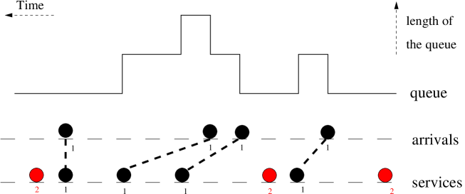
Figure 2: Queueing picture for the two species case. Here time $t(i)=L-i$ increases from right to left, where $i$ is site number.

We recall (see e.g. Figure 2) that a 2-line configuration generates a 2-TASEP configuration. Since, as described above, the stationary state factorises about the positions of the second-class particles we only need to consider a binary string $B$ of 1s and 0s between two 2s in a 2-TASEP configuration. There are several 2-line configurations which generate the string $B$. Those 2-line configurations must satisfy two conditions: (a) both lines 1 and 2 must contain the same number of particles, equal to the number of 1s in $B$ and (b) line 2 coincides with $B$. The possibilities for line 1 are then generated from line 2 by pushing particles to the right. For example, the lower line of Figure 2 has three strings of type $B$ delimited by the three second class particles: $B_{0}=0$, $B_{1}=1010100$ and $B_{2}=100$. The upper-line string $1000011$ is one of the strings producing $B_{1}$, the string $010$ is one of the strings producing $B_{2}$ and the string $0$ is the only string producing $B_{0}$.

Given a 2-line configuration one can associate to it the trajectory of the length of a queue. Consider the labels of the particles of line 2 as first or second class particles as given by Angel’s algorithm (illustrated in Figure 1). Time for the queue runs from right to left: at each site $i$ it is assigned a time $t(i)=L-i$. The queue has length zero at the times corresponding to the positions of second class particles in line 2 (unused service times), a particle in line 1 represents an arrival time and a first class particle in line 2 represents a service time. At a given time $t(i)$ the length of the queue (constrained to be non-negative) increases by one when a particle is present at site $i$ in line 1 but not in line 2 (a new arrival occurs and is not serviced); the length of the queue decreases by one when a particle is present in line 2 but not in line 1 (a service occurs with no new arrival). If no particles are present in lines 1 and 2 (no service or new arrival occurs) or when particles are present in both lines 1 and 2 (a new arrival occurs and is serviced) the queue remains at the same length. The weight of a 2-TASEP string is then given by all possible queue trajectories, consistent with following constraints i) the queue has length zero at the positions of the second class particles ii) the effective service times of the queue are fixed by the positions of the first class particles. Since the full 2-line configuration can be retrieved by knowing the 2-TASEP configuration and the trajectory of the queue, to enumerate the ancestors of a 2-TASEP configuration it is enough to enumerate the queue trajectories compatible with it.

We now illustrate how the product of matrices $A$, $D$, $E$ defined in (11,12,13) precisely enumerates the possible trajectories of the queue giving rise to a given 2-TASEP configuration. The right hand vector $|0\rangle$ represents an initial queue length of 0. At each service time of the queue we have a matrix $D$ and at each non-service time a matrix $E$. A vector $|n\rangle$ represents the length of the queue. If the length of the queue just before a service time is $n>0$ the action of $D$ on $|n\rangle$ is

$$D|n\rangle=|n\rangle+|n-1\rangle\;.$$ (42)

The two terms represent the two possibilities at the service time: the first represents the service of a new arrival at that time, the second represents a service and no new arrival. If $n=0$,

$$D|0\rangle=|0\rangle$$ (43)

which implies that a new arrival has to be serviced at this time, otherwise there would be an unused service which is forbidden.

Similarly, if the length of the queue is $n\geq 0$ just before a non-service time, the action of $E$ on $|n\rangle$ is

$$E|n\rangle=|n\rangle+|n+1\rangle\;.$$ (44)

The first term represents no new arrival at that time, the second term represents a new arrival at that time.

The projector $|0\rangle\langle 0|$ at the left end of the string ensures that only trajectories of the queue which finish at length 0 are counted and the queue length is set to 0 for the start of the next string.

Remarks

1. An alternative way to determine the queue length $n$ at a given time $t(i)=L-i$ is the following. In Figure 2 each particle in line 1 is associated to a particle in line 2 by a dashed black line. The length of the queue at $t(i)$ is given by the number of dashed black lines intersecting a vertical segment passing through $i^{-}$, i.e. just to the left of site $i$; vertical dashed black lines do not affect the queue length.

2. The trajectory of the length of the queue in the queueing process with constraints described above is precisely a Motzkin path. This allows one to represent matrix product calculations in terms of ensembles of Motzkin paths see e.g. [22, 23, 24].

3 The ${N}$-Species TASEP

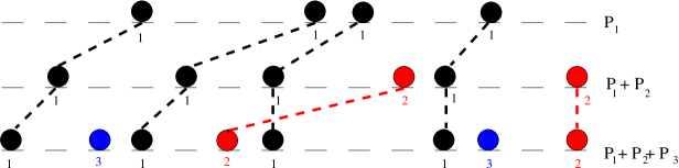
Figure 3: Graphical representation of Ferrari-Martin’s algorithm.

3.1 Construction for ${N}$ Species of Particle

In this section we review how the construction for the 2-species case is extended to the ${N}$-species case [17]. For ${N}$ species of particle we consider ${N}$-line configurations of particles. The first line comprises $P_{1}$ particles distributed randomly (with at most one particle per site). The second line comprises $P_{1}+P_{2}$ particles distributed randomly and so on until the ${N}$th line which comprises $P_{1}+P_{2}\cdots+P_{N}$ particles distributed randomly. Initially, in this ${N}$-line configuration, particles are not differentiated into species. In the following we define the construction by which a species label is attributed to each of the particles. Once this has been done the ${N}$th line is identified with an ${N}$-TASEP configuration.

We start with line 1 and associate each particle in line 1 to a particle in line 2 as in Section 2.1. This is done by beginning with a particle in line 1 and associating it with the nearest particle, at the same site or to the left, in line 2. We then take the next particle to the left in line 1 and associate it in the same way to the first unassociated particle in line 2. This process is continued until each of the particles in line 1 is associated with one particle in line 2. These $P_{1}$ particles in line 2 are then labelled 1 and the remaining $P_{2}$ unassociated particles in line 2 are labelled 2. The resulting labels do not depend on which particle we began with in line 1, as commented in Section 2.1.

We now proceed to associate the particles in line 2 with those in line 3. First we use the same procedure as described above to associate the particles labelled 1 in line 2 each to a particle in line 3. The $P_{1}$ associated particles in line 3 are then labelled 1. We then proceed to associate the particles labelled 2 in line 2 to $P_{2}$ of the unassociated particles in line 3 (ignoring the particles already labelled 1 in line 3). These particles in line 3 are then labelled 2 and the remaining $P_{3}$ unassociated particles in line 3 are labelled 3.

The procedure is then repeated up to line ${N}$ and results in $P_{K}$ of the particles in line ${N}$ having label $K$ where $1\leq K\leq{N}$. The construction is illustrated by an example in the three species case in Fig. 3. Starting from the random distributions of particles in the ${N}$ lines, one obtains a configuration of the ${N}$ species TASEP with $P_{K}$ particles of species $K$. The probability of the ${N}$-TASEP configuration so obtained is equal to its stationary probability under the ${N}$-TASEP dynamics. This was proven in [17]; in Section 4.4 we shall give an alternative proof, based on the matrix formulation, for the 3-TASEP.

Our aim is now to invert this construction. That is, for a given ${N}$-TASEP configuration, we wish to compute the probability that it is generated by the above procedure. This amounts to the combinatorial problem of counting the number of ways particles may be distributed in the ${N}$-line configuration such that the construction will lead to the desired ${N}$-TASEP configuration.

As has been discussed in Section 2.1, for the 2 species case Angel [15] gave such a construction and this is equivalent to the matrix product approach of Derrida et al [12] (see section 2.2). We showed this by using the queueing representation of Ferrari and Martin. In the following we first provide an algorithm, generalising the pushing procedure of Section 2 by which the probabilities can be computed. We then construct explicit matrices which compute the ${N}$-TASEP weights by book-keeping the generalized pushing procedure.

3.2 Ferrari and Martin’s Construction and the Reverse Algorithm

As described above, in the ${N}$-species procedure of Ferrari and Martin a configuration of the ${N}$-TASEP is obtained from an ${N}$-line configuration, where each of the ${N}$ lines consists of a single species TASEP configuration. The procedure may be viewed in the following way: from line 1 (a configuration of the single species TASEP) and line 2 one obtains a uniquely defined configuration of the 2-TASEP; from that configuration of the 2-TASEP and line 3 one constructs a configuration of the 3-TASEP and so on, until one reaches a configuration of the ${N}$-TASEP. Therefore, a given configuration of the ${N}$-TASEP arises from a whole set of (${N}-1$)-TASEP configurations that we shall call its ancestors; each of these (${N}-1$)-TASEP configurations arises in turn from a whole set of (${N}-2$)-TASEP ancestors etc…

The stationary weight of the initial ${N}$-TASEP configuration is then given (but for an overall normalization constant) by the sum of the weights of the (${N}-1$)-TASEP configurations that lead to it (its ancestors). Applying this procedure recursively, we observe that this stationary weight is given by the sum of the weights of its (${N}-2$)-TASEP ancestor configurations. Finally, because the single species TASEP has a uniform steady state, the weight of any ${N}$-TASEP configuration is nothing but the total number of configurations of the single species TASEP from which it derives. Therefore, to calculate the weight of a given ${N}$-TASEP configuration we must determine the total number of 1-TASEP configurations that are its ancestors.

In the following we shall give a recursive algorithm to determine all the $({N}-1)$-TASEP ancestors of a given ${N}$-TASEP configuration. Iterating this algorithm it is possible to obtain the total number of 1-TASEP ancestors of a given ${N}$-TASEP configuration; this number corresponds to the stationary weight of the ${N}$-TASEP configuration.

In order to simplify our discussion we shall first present this algorithm for the case of a 3-TASEP configuration, i.e. for a string of particles of classes 1, 2, 3 and holes (denoted by 0). We start from an initial 3-TASEP configuration.

1. Freeze the positions of the 2s and the 3s. Construct all possible configurations obtained by pushing the 1s through the holes towards the right, until they hit a 2 or a 3 (i.e. a 1 can cross neither a 2 nor a 3). $\rightarrow$ This procedure leads to many 3-TASEP configurations with various positions of the 1s. From now on the sites where the 1s are located will be passive.

2. Keep the positions of the 3s frozen and start moving the 2s. For each configuration obtained above, construct all possible configurations obtained by pushing the 2s through the holes towards the right, until they hit a 3. Note that the sites occupied by 1s are spectators and the 2s hop over them as if they do not exist. $\rightarrow$ This procedure leads to many 3-TASEP configurations in which the positions of the 1s and the 2s are fixed.

3. Replace all the 3s by holes. We thus have obtained the complete set of 2-TASEP ancestors of the initial 3-TASEP configuration we started with.

4. The stationary weight of the initial 3-TASEP configuration (up to a global normalization constant) is the sum of the weights of its 2-TASEP ancestors.

Let us illustrate the algorithm with the explicit example of the string 2103

1. By pushing 1s to the right we obtain the strings 2103, 2013

2. By pushing 2s to the right (through the 1s), from 2103 we obtain 2103 and 0123 and from 2013 we obtain 2013 and 0213

3. We replace 3s by 0s to obtain the strings 2100, 0120, 2010, 0210

4. The weight of string 2103 in the 3-TASEP in terms of 2-TASEP weights is given by

   $$W(2103)\,=\,W(2100)+W(0120)+W(2010)+W(0210),$$

   which we may calculate, for example by using the matrix ansatz for the 2-TASEP (8–10) and (38), as $W(2103)=3+1+2+3=9$.

It is easy to generalise to the ${N}$-species case and compute the weight of a ${N}$-TASEP configuration in terms of the weights of $({N}{-}1)$-TASEP configurations

1. Freeze the positions of the species $2,\ldots,K$. Construct all possible configurations obtained by pushing the 1s through the holes towards the right (a 1 cannot cross any species of particle).

2. Now in turn for $K=2,\ldots,N-1$ push species $K$ to the right keeping the positions of species $K+1,\ldots,N$ frozen and with species $1,\ldots,K-1$ spectators. i.e. For each configuration obtained from step 1, construct all possible configurations obtained by pushing the 2s through the holes to the right, allowing the 2s to hop over 1s; then push 3s to the right allowing 3s to hop over 2s and 1s, and so on until species $K-1$ have been pushed to the right, hopping over all other species except $K$.

3. In all of the ${N}$-TASEP configurations generated in step (ii), replace all the ${N}$s by holes. We thus have obtained a whole set of $({N}{-}1)$-TASEP configurations: this is the complete set of ancestors of the initial ${N}$-TASEP configuration we started with.

4. The sum of the stationary weight of all these $({N}{-}1)$-TASEP ancestor configurations gives the stationary weight of the ${N}$-TASEP configuration.

We saw that ‘the pushing procedure’ of Angel is naturally implemented by the $D,E$ and $A$ matrices. The algorithm given above is also based on recursive pushing procedures and as we shall show in section 4.2 can be encoded by a matrix ansatz; in this case the matrices for the ${N}$-TASEP are built by using the matrices for the $({N}{-}1)$-TASEP as elements.

3.3 Queueing Interpretation of ${N}$-Species Construction

Ferrari and Martin also proposed a queueing interpretation for the multiline construction. The ${N}$ lines of the ${N}$-species construction correspond to ${N}-1$ queues. The first line represents arrival times to the queue 1. The second line represents service times for queue 1. We continue using the convention that the queue time runs from right to left, so that the time $t(i)$ associated to site $i$ is given by $t(i)=L-i$. As we have seen in section 2.3, unused service times of queue 1 become second-class particles. Then when the particles of line 2 have been labelled either first or second-class, they represent the arrivals for queue 2. The arrivals are distinguished into first and second-class and the queue is a priority queue: at the service times (given by the particles in line 3) the highest priority waiting customer is always serviced first. That is, in queue 2 first-class arrivals are served before second-class arrivals. The ouput of these service times then become the arrival times for queue 3 with unused service times in queue 2 providing third-class arrivals to queue 3. This construction is iterated until the particles in line ${N}-1$, labelled $1,\ldots{N}-1$ provide the arrivals for queue ${N}-1$ and the particles in line ${N}$ provide the service times for queue ${N}-1$. When the particles in line ${N}$ are labelled $1\ldots{N}$ they become the output of queue ${N}-1$, which corresponds to the ${N}$-TASEP configuration.

4 The Matrix Product Formulation

In this section, we show how the recursive construction for the ${N}$-TASEP, described in Section 3.2, can be encoded within the matrix product formulation, described in Section 2.2.

4.1 Definition of the Matrix Product Ansatz and Simple Examples

The matrix ansatz [9] provides a solution to the stationary master equation of the ${N}$-TASEP (made explicit later in (101)), as follows. First consider non-commuting matrices $X_{0},X_{1},\ldots,X_{N}$, where $X_{K}$ is associated to particles of class $K$ (in particular $X_{0}$ is associated to holes, $X_{1}$ is associated to first-class particles etc…). The ansatz represents the stationary probability ${\rm P}({\cal C})$ of a ${N}$-TASEP configuration ${\cal C}=(\tau_{1},\dots,\tau_{L})$ (where $\tau_{i}$ is equal to $K$ if site $i$ is occupied by a particle of class $K$) as a statistical weight $W({\cal C})$ divided by a normalization $Z$

$${\rm P}({\cal C})=\frac{1}{Z}W({\cal C})$$ (45)

where the weight is given by the trace of the product of $L$ matrices, as follows

$$W({\cal C})={\rm Tr}(X_{\tau_{1}}...X_{\tau_{L}})\;.$$ (46)

Here $X_{\tau_{i}}$ is equal to $X_{K}$ if site $i$ is occupied by a particle of class $K$ $(K=0,1,\ldots,N)$ in configuration ${\cal C}$. The normalization factor $Z$ (that depends on $L$ and on all the $P_{K}$’s where $P_{K}$ represents the total number of particles of class $K$) ensures that $\sum_{\cal C}{\rm P}({\cal C})=1$. We emphasize that the matrix formulation depends on the number of species. For example the matrices that represents first-class particles in the 2-TASEP and the 3-TASEP are not the same.

If the system contains only first-class particles and holes, it is well known that the stationary measure is uniform. Thus the particles and the holes may both be represented by one (a scalar) and the matrix ansatz reduces here to a trivial form.

For the 2-TASEP holes, first-class and second-class particles are represented respectively by the matrices $X_{0}=E$, $X_{1}=D$ and $X_{2}=A$ (in the notation of [9, 12]) which satisfy (8,9,10). It is convenient to introduce matrices $\epsilon$ and $\delta$ defined by

$$E={\bf 1}+\epsilon,\,\,\,\,\,\,D={\bf 1}+\delta\,\,$$ (47)

where ${\bf 1}$ is the identity matrix. Then, by (8,9,10), the matrices $\epsilon,A,\delta$ generate the following quadratic algebra:

$$\delta\epsilon = {\bf 1}$$

$$\delta A = 0$$

$$A\epsilon = 0\;.$$ (48)

4.2 Matrix Ansatz for 3-TASEP

We now present the matrix product formulation of the stationary state of the 3-TASEP.

$$X_{1} = {\bf 1}\otimes{\bf 1}\otimes D+\delta\otimes\epsilon\otimes A+\delta\otimes{\bf 1}\otimes E$$ (49)

$$X_{2} = A\otimes{\bf 1}\otimes A+A\otimes\delta\otimes E$$ (50)

$$X_{3} = A\otimes A\otimes E$$ (51)

$$X_{0} = {\bf 1}\otimes{\bf 1}\otimes E+{\bf 1}\otimes\epsilon\otimes A+\epsilon\otimes{\bf 1}\otimes D\,.$$ (52)

Note that the matrices are generally sums of tensor products of three semi-infinite matrices used in the matrix product representation of the stationary state of the 2-TASEP. From the usual representation of the matrices $A,\delta$ and $\epsilon$ given in [9, 12] we obtain explicit expressions for the above matrices: they all have a block structure that is bidiagonal. Defining matrices $F$, $G$, $H$ and ${R}$ as

$$F=\left(\begin{array}[]{ccccc}D&0&0&0&\dots\\ 0&D&0&0&\ddots\\ 0&0&D&0&\ddots\\ 0&0&0&D&\ddots\\ \vdots&\ddots&\ddots&\ddots&\end{array}\right)\qquad G=\left(\begin{array}[]{ccccc}E&0&0&0&\dots\\ A&E&0&0&\ddots\\ 0&A&E&0&\ddots\\ 0&0&A&E&\ddots\\ \vdots&\ddots&\ddots&\ddots&\end{array}\right)$$ (63)

$$H=\left(\begin{array}[]{ccccc}A&E&0&0&\dots\\ 0&A&E&0&\ddots\\ 0&0&A&E&\ddots\\ 0&0&0&A&\ddots\\ \vdots&\ddots&\ddots&\ddots&\end{array}\right)\qquad{R}=\left(\begin{array}[]{ccccc}E&0&0&0&\dots\\ 0&0&0&0&\ddots\\ 0&0&0&0&\ddots\\ 0&0&0&0&\ddots\\ \vdots&\ddots&\ddots&\ddots&\end{array}\right)$$ (74)

the matrix representation of (49–52) reads

$$X_{1}=\left(\begin{array}[]{ccccc}F&G&0&0&\dots\\ 0&F&G&0&\ddots\\ 0&0&F&G&\ddots\\ 0&0&0&F&\ddots\\ \vdots&\ddots&\ddots&\ddots&\end{array}\right)\qquad X_{2}=\left(\begin{array}[]{ccccc}H&0&0&0&\dots\\ 0&0&0&0&\ddots\\ 0&0&0&0&\ddots\\ 0&0&0&0&\ddots\\ \vdots&\ddots&\ddots&\ddots&\end{array}\right)$$ (85)

$$X_{3}=\left(\begin{array}[]{ccccc}{R}&0&0&0&\dots\\ 0&0&0&0&\ddots\\ 0&0&0&0&\ddots\\ 0&0&0&0&\ddots\\ \vdots&\ddots&\ddots&\ddots&\end{array}\right)\qquad X_{0}=\left(\begin{array}[]{ccccc}G&0&0&0&\dots\\ F&G&0&0&\ddots\\ 0&F&G&0&\ddots\\ 0&0&F&G&\ddots\\ \vdots&\ddots&\ddots&\ddots&\end{array}\right)$$ (96)

All these matrices are triply infinite dimensional because their coefficients are themselves infinite dimensional matrices with elements $D$, $A$ and $E$ (which are also infinite dimensional matrices).

4.3 Matrices as Priority Queue Matrices

We now explain in the case ${N}=3$ how these matrices may be obtained from the ${N}$-species queueing interpretation of the ${N}$-line configuration discussed in section 3.3. In this case we have a 3-line configuration that represents two queues in tandem. Queue 1 has one type of customer which are considered to be first-class: Line 1 represents the arrival times of (first-class) customers in queue 1 and line 2 gives the service times of queue 1. The particles of line 2 are labelled 1 or 2 according to whether a service time is used or unused. Once labelled, the particles of line 2 become the arrival times to queue 2. Queue 2 is a priority queue containing first and second-class customers: any first-class customer is served before the second-class customers waiting in the queue. The particles of line 3 are the service times for queue 2. They are labelled by which class of customer is served; if a service is unused it is labelled 3.

We now consider the possible trajectories of the queue system. To do this we require 3 integer counters $l,m,n$: $l$ is the number of first-class customers waiting in queue 2; $m$ is the number of second-class customers waiting in queue 2; $n$ is the number of first-class customers waiting in queue 1 (i.e. the length of queue 1). The three counters indicate the state of the system at each queue time $t(i)=L-i$ (which runs from right to left). The counters are therefore indexed by the times $t(i)$ associated to sites $i$, but we omit this in our notation.

Remark: The values of the counters can be obtained directly from figure 3 as follows: for each site $i$, the counter $l$ with index $t(i)$ represents the number of black dashed lines crossing a vertical segment passing through $i^{-}$ between lines $2$ and $3$; $m$ represents the number of red dashed lines crossing the same segment and $n$ represents the number of black dashed lines crossing the segment between lines $1$ and $2$; vertical dashed lines are not counted at all. The queue counters do not register (a) second class particles served at their arrival time, (b) first class particles served in both queues at their arrival time and (c) unused services in the third line. However, a 3-TASEP configuration and the trajectories of the three queues uniquely determine the 3-line configuration generating it. This implies that it is enough to enumerate the set of queues trajectories compatible with the 3-TASEP configuration we are computing the weight of.

The queue counters $l,m,n$ can be represented by a state vector $|l\,m\,n\rangle$

$$|l\,m\,n\rangle\equiv|l\rangle\otimes|m\rangle\otimes|n\rangle$$ (97)

where $|l\rangle=0$ for $l<0$. We show now that the matrix product using $X_{0},X_{1},X_{2},X_{3}$ defined in (49–52) precisely enumerate the possible trajectories of the state of the tandem queues giving rise to a given configuration $(\tau_{1},\dots,\tau_{L})$.

We list the possible updates of the counters $l,m,n$ at a given site (or time), according to the line 3 label of that site, i.e. the site variable $\tau_{i}$ in the ${N}$-TASEP configuration. Then from each possible update of the queue lengths we deduce the necessary action of the matrices $X_{i}$, $i=0,1,2,3$, on the state vector $|l\,m\,n\rangle$. Finally we can check from the definitions (49–52) of the actions of $D$,$E$,$A$ (42,43,44) that $X_{i}|l\,m\,n\rangle$ produces the required update of the queue counters.

$\tau_{i}=3$

In this case there is an unused service in queue 2 which implies $l=m=0$. In queue 1 there may or may have not been an arrival therefore $n\to n$ or $n\to n+1$. Thus, the action of $X_{3}$ must be

$$X_{3}|l\,m\,n\rangle=\delta_{l,0}\delta_{m,0}|0\rangle\otimes|0\rangle\otimes\left[|n\rangle+|n+1\rangle\right]=A\otimes A\otimes E|l\,m\,n\rangle$$ (98)

which recovers the matrix expression for $X_{3}$, (51).

$\tau_{i}=2$

In this case a second-class service occurs in queue 2 which implies that the number of first-class customers $l=0$ and there is no first-class arrival in queue 2. If there were a second-class arrival in queue 2 so that $m\to m$, it would imply $n=0$ as there would have to be an unusued service in queue 1. On the other hand, if there were no second-class arrival at queue 2 so that $m\to m-1$ then there might or might not be a first-class arrival at queue 1 and $n\to n$ or $n\to n+1$. Thus, the action of $X_{2}$ must be

$$X_{2}|l\,m\,n\rangle =\delta_{l,0}|0\rangle\otimes\left[\,\delta_{n,0}|m\rangle\otimes|0\rangle+|m-1\rangle\otimes\left[|n\rangle+|n+1\rangle\right]\,\right]$$ (99)

$$=\left[A\otimes{\bf 1}\otimes A+A\otimes\delta\otimes E\right]|l\,m\,n\rangle$$ (100)

which recovers the matrix expression for $X_{2}$, (50).

$\tau_{i}=1$

In this case a first-class service occurs in queue 2. If there is also a first-class arrival at queue 2 then $l\to l$, $m\to m$ and $n\to n-$1 or $n$ since there is a first-class service and possibly a first-class arrival at queue 1. If there is instead a second-class arrival at queue 2 (a second-class service in queue 1) then there must be no first-class customers in queue 1 and so $l\to l-1$, $m\to m+1$ and $n=0$. Finally, if there is no arrival to queue 2 then there is no departure from queue 1 and there may or may not be an arrival at queue 1. Therefore $l\to l-1$, $m\to m$ and $n\to n$ or $n+1$.

Thus, the action of $X_{1}$ must be

$$X_{1}|l\,m\,n\rangle = |l\rangle\otimes|m\rangle\otimes\left[|n\rangle+|n-1\rangle\right]+|l-1\rangle\otimes|m+1\rangle\otimes|0\rangle\delta_{n,0}$$

$$+|l-1\rangle\otimes|m\rangle\otimes\left[\,|n\rangle+|n+1\rangle\,\right]$$

$$= |l\rangle\otimes|m\rangle\otimes D|n\rangle+\delta|l\rangle\otimes\epsilon|m\rangle\otimes A|n\rangle+\delta|l\rangle\otimes|m\rangle\otimes E|n\rangle$$

$$= \left[{\bf 1}\otimes{\bf 1}\otimes D+\delta\otimes\epsilon\otimes A+\delta\otimes{\bf 1}\otimes E\right]|l\,m\,n\rangle$$

which recovers the matrix expression for $X_{1}$, (49).

$\tau_{i}=0$

In this case there is no service at queue 2. If there is first-class arrival at queue 2 $l\to l+1$, $m\to m$ and $n\to n-1$ or $n$ since there is a first-class service and possibly a first-class arrival at queue 1. If there is instead a second-class arrival at queue 2 (a second-class service in queue 1) then there must be no first-class customers in queue 1 and so $l\to l$, $m\to m+1$ and $n=0$. Finally, if there is no arrival at queue 2 then there is no departure from queue 1 and there may or may not be an arrival at queue 1. Therefore $l\to l$, $m\to m$ and $n\to n$ or $n+1$. Thus, the action of $X_{1}$ must be

$$X_{0}|l\,m\,n\rangle = |l+1\rangle\otimes|m\rangle\otimes\left[\,|n\rangle+|n-1\rangle\,\right]+|l\rangle\otimes|m+1\rangle\otimes|0\rangle\delta_{n,0}$$

$$+|l\rangle\otimes|m\rangle\otimes\left[\,|n\rangle+|n+1\rangle\,\right]$$

$$= \epsilon|l\rangle\otimes|m\rangle\otimes D|n\rangle+|l\rangle\otimes\epsilon|m\rangle\otimes A|n\rangle+|l\rangle\otimes|m\rangle\otimes E|n\rangle$$

$$= \left[\epsilon\otimes{\bf 1}\otimes D+{\bf 1}\otimes\epsilon\otimes A+{\bf 1}\otimes{\bf 1}\otimes E\right]|l\,m\,n\rangle$$

which recovers the matrix expression for $X_{0}$, (52).

4.4 Algebraic Proof of the Matrix Product Ansatz

The matrix product ansatz may be proved independently of the queueing representation in an algebraic way. We shall use the technique of “hat matrices” to prove the ansatz (see e.g., [20, 25, 26] for more details).

We first recall the stationarity condition to be satisfied. The dynamics of the system can be encoded in a Markov matrix ${Q}$ of size $\Omega\times\Omega$ where $\Omega$ is the total number of configurations of the system. The coefficient ${Q}({\cal C},{\cal C}^{\prime})$ of this matrix represents the rate of transition from a configuration ${\cal C}^{\prime}$ to a different configuration ${\cal C}$; $-{Q}({\cal C},{\cal C})$ is the total rate of exit from a given configuration ${\cal C}$. (Notice that this is the transpose of the usual generator matrix used in probability.) Thus the stationary probabilities must satisfy the stationary master equation

$$\sum_{{\cal C}^{\prime}}{Q}({\cal C},{\cal C}^{\prime}){\rm P}({\cal C^{\prime}})=0\,\,\,\,.$$ (101)

Due to the local structure of the rules (1,2), ${Q}$ can be written as a sum of local matrices that represent the transitions that take place at a bond $(i,i+1)$

$${Q}=\sum_{i=1}^{L}{Q}_{i,i+1}\,\,\,\,.$$ (102)

${Q}_{i,i+1}$ are $(N+1)^{2}\times(N+1)^{2}$ matrices whose off diagonal elements ${Q}_{i,i+1}(\tau_{i}\tau_{i+1};\tau_{i}^{\prime}\tau_{i+1}^{\prime})$ give the transition rate from configuration $\tau^{\prime}_{i}\tau^{\prime}_{i+1}$ to $\tau_{i}\tau_{i+1}$ at the bond $i,i+1$, and whose diagonal element ${Q}_{i,i+1}(\tau_{i}\tau_{i+1};\tau_{i}\tau_{i+1})$ gives minus the total transition rate out of configuration $\tau_{i}\tau_{i+1}$. Since the only transitions involved in the $N$-TASEP are exchanges at a bond, we have

$${Q}_{i,i+1}(JK,KJ)=-{Q}_{i,i+1}(KJ,KJ)=1,\; \hbox{if }K\geq 1\hbox{ and }J>K\hbox{ or }J=0\,,$$

$${Q}_{i,i+1}(K^{\prime}J^{\prime},KJ)=0,$$ otherwise,

where here $K,J$ are indices that take values from 0 to ${N}$. When the steady state probabilities are written in the matrix product form (45) the local matrix ${Q}_{i,i+1}$ acts only on the $i$th and the $(i+1)$th matrices in the product. The stationarity condition (101) then may be written

$$\sum_{i=1}^{L}{\rm Tr}(X_{\tau_{1}}\ldots X_{\tau_{i-1}}Y_{\tau_{i},\tau_{i+1}}X_{\tau_{i+2}}\ldots X_{\tau_{L}})=0$$ (103)

where

$$Y_{\tau_{i},\tau_{i+1}}=\sum_{\tau_{i}^{\prime},\tau_{i+1}^{\prime}}{Q}_{i,i+1}(\tau_{i}\tau_{i+1};\tau_{i}^{\prime}\tau_{i+1}^{\prime})X_{\tau_{i}^{\prime}}X_{\tau_{i+1}^{\prime}}\;.$$ (104)

That is,

$$\begin{array}[]{ll}Y_{KJ}=-X_{K}X_{J}&\hbox{for all}\quad K\geq 1\hbox{ and }J>K\hbox{ or }J=0\,,\\ Y_{JK}=X_{K}X_{J}&\hbox{for all}\quad K\geq 1\hbox{ and }J>K\hbox{ or }J=0\,,\\ Y_{JJ}=0&\hbox{for all}\quad J\;.\end{array}$$ (105)

The key point to prove the validity of the matrix ansatz is to show that $Y_{\tau_{i},\tau_{i+1}}$ is a divergence-like term, i.e. there exist matrices ${\hat{X}_{\tau}}$ such that

$$Y_{\tau_{i},\tau_{i+1}}=X_{\tau_{i}}{\hat{X}_{\tau_{i+1}}}-{{\hat{X}_{\tau_{i}}}}X_{\tau_{i+1}}\,.$$ (106)

Summation over $i$ leads to a global cancellation in (103), proving thereby that the stationarity condition (101) is satisfied. Combining (105,106), we obtain the conditions:

$$X_{K}X_{J} = \hat{X}_{K}X_{J}-X_{K}\hat{X}_{J}\quad\quad\hbox{for all}\quad K\geq 1\hbox{ and }J>K\hbox{ or }J=0\,,$$ (107)

$$X_{K}X_{J} = X_{J}\hat{X}_{K}-\hat{X}_{J}X_{K}\quad\quad\hbox{for all}\quad K\geq 1\hbox{ and }J>K\hbox{ or }J=0\,,$$ (108)

$$0 = X_{J}\hat{X}_{J}-\hat{X}_{J}X_{J}\quad\quad\;\,\hbox{for all}\quad J.$$ (109)

For $N=2$, it turns out to be rather easy to solve the above equations (see e.g. [20]): indeed, one finds that (107–109) may be satisfied by choosing ${\hat{X}_{\tau}}$ to be scalars so that they commute with ${X_{\tau}}$. Then (109) is immediately satisfied and (107,108) reduce to 3 conditions

$$X_{1}X_{0} = {\hat{X}_{1}}X_{0}-{\hat{X}_{0}}X_{1}$$ (110)

$$X_{1}X_{2} = {\hat{X}_{2}}X_{1}-{\hat{X}_{1}}X_{2}$$ (111)

$$X_{2}X_{0} = {\hat{X}_{2}}X_{0}-{\hat{X}_{0}}X_{2}\;.$$ (112)

Choosing ${\hat{X}_{1}}=+1$, ${\hat{X}_{0}}=-1$, ${\hat{X}_{2}}=0$ and $X_{1}=D$, $X_{0}=E$, $X_{2}=A$ recovers (8–10).

For $N=3$ it turns out that choosing ${\hat{X}_{\tau}}$ to be scalars does not allow (107–108) to be satisfied. Thus, the proof rests upon finding the $4$ matrices ${\hat{X}}_{K}$ for $K=0,1,2,3$. We now write explicit forms for the hat matrices that fulfil the above relations when $X_{K}$ are given by (49–52):

$$\hat{X}_{1} = ({\bf 1}-\delta)\otimes{\bf 1}\otimes{\bf 1}$$

$$\hat{X}_{2} = -A\otimes\delta\otimes{\bf 1}$$

$$\hat{X}_{3} = -A\otimes A\otimes{\bf 1}$$

$$\hat{X}_{0} = -X_{0}+(\epsilon-{\bf 1})\otimes{\bf 1}\otimes{\bf 1}\;.$$ (113)

It remains to verify that relations (107,108,109) are satisfied. Here we check a few relations involving $X_{1}$ and $\hat{X}_{1}$. For $J=1$ the rhs of (109) becomes

$$X_{1}\hat{X}_{1}-\hat{X}_{1}X_{1} = ({\bf 1}-\delta)\otimes{\bf 1}\otimes D+\delta({\bf 1}-\delta)\otimes\epsilon\otimes A+\delta({\bf 1}-\delta)\otimes{\bf 1}\otimes E$$

$$- ({\bf 1}-\delta)\otimes{\bf 1}\otimes D-({\bf 1}-\delta)\delta\otimes\epsilon\otimes A-({\bf 1}-\delta)\delta\otimes{\bf 1}\otimes E=0\;.$$

Thus (109) is satisfied in the case $J=1$.

Using relations (48) we find

$$X_{1}X_{2}=A\otimes{\bf 1}\otimes DA+A\otimes\delta\otimes DE=A\otimes{\bf 1}\otimes A+A\otimes\delta\otimes(D+E)\;,$$

and

$$\hat{X}_{1}X_{2}-X_{1}\hat{X}_{2} = A\otimes{\bf 1}\otimes A+A\otimes\delta\otimes E-(-A\otimes\delta\otimes D)$$

$$= X_{1}X_{2}$$

$$X_{2}\hat{X}_{1}-\hat{X}_{2}X_{1} = A({\bf 1}-\delta)\otimes{\bf 1}\otimes A+A({\bf 1}-\delta)\otimes\delta\otimes E+$$

$$-(-A\otimes\delta\otimes D-A\delta\otimes\delta\epsilon\otimes A-A\delta\otimes\delta\otimes E)\;,$$

$$= X_{1}X_{2}$$

thus (107,108) are satisfied for the case $K=1$, $J=2$. Similarly, all relations (107,108,109) may be verified.

5 Hierarchical Matrix Ansatz for the Multispecies ASEP

In this section, we generalize the previous construction to the multispecies totally asymmetric exclusion process on the ring ${\mathbb{Z}}_{L}$ with ${N}$ classes of particles for any ${N}>1$. We show that a matrix ansatz for a system containing ${N}$ classes of particles (plus holes) can be constructed recursively knowing a matrix ansatz for a system with ${N}-1$ classes of particles (plus holes). We shall simply present the results here and give some examples; we leave the algebraic proof and further generalizations to a future publication.

The matrices $X_{K}^{({N})}$ at level ${N}$ are obtained by making tensor products of the $X_{M}^{({N}-1)}$ defined at level ${N}-1$ with some matrices $a_{KM}$ constructed from $\epsilon,A,\delta$ and ${\bf 1}$. The matrix ansatz is given by

$$X_{0}^{({N})} = \sum_{M=0}^{{N}-1}a_{0M}^{({N})}\otimes X_{M}^{({N}-1)}$$ (114)

$$X_{K}^{({N})} = a_{K0}^{({N})}\otimes X_{0}^{({N}-1)}+\sum_{M=K}^{{N}-1}a_{KM}^{({N})}\otimes X_{M}^{({N}-1)}\,\,\,\,\,\hbox{ for }1\leq K\leq{N}\;.$$ (115)

We emphasize that in this section our notation for the matrix $X_{K}^{({N})}$ has two indices: the lower index $K$ denotes the class of the particle represented by the matrix, whereas the upper index ${N}$ gives the total number of classes considered in the system.

The fundamental building blocks to construct the $a_{KM}^{({N})}$ matrices are the matrices $\epsilon,A,\delta$ and ${\bf 1}$ (identity). The $a_{KM}^{({N})}$ are then given by

$$a_{00}^{({N})} = {\bf 1}^{\otimes({N}-1)}$$ (116)

$$a_{0M}^{({N})} = {\bf 1}^{\otimes(M-1)}\otimes\epsilon\otimes{\bf 1}^{\otimes({N}-M-1)}\,\,\,\hbox{ for }1\leq M\leq{N}-1\;.$$ (117)

For $K\geq 1$ we have

$$a_{K0}^{({N})} = A^{\otimes(K-1)}\otimes\delta\otimes{\bf 1}^{\otimes({N}-K-1)}\,\,\,\hbox{ for }1\leq K\leq{N}-1$$ (118)

$$a_{KK}^{({N})} = A^{\otimes(K-1)}\otimes{\bf 1}^{\otimes({N}-K)}$$ (119)

$$a_{KM}^{({N})} = A^{\otimes(K-1)}\otimes\delta\otimes{\bf 1}^{\otimes(M-K-1)}\otimes\epsilon\otimes{\bf 1}^{\otimes({N}-M-1)}\,\,\,\hbox{ for }1\leq K<M\leq{N}-1{\hskip 21.33955pt}$$ (120)

$$a_{{N}0}^{({N})} = A^{\otimes({N}-1)}\;.$$ (121)

It is understood in the formulae above that any matrix raised to a tensor-power equal to zero is equal to the scalar 1 which can be removed from the tensor product.

Note from (114,115) that the matrices $X_{K}^{({N})}$ at level ${N}$ are composed of tensor products of ${{{N}}\choose 2}$ fundamental matrices $\epsilon,A,\delta$ or ${\bf 1}$.

5.1 Some Examples

Using the hierarchical matrix ansatz given above, we study explicitly the cases ${N}\leq 3$.

For ${N}=0$, the system does not contain any particles but only holes. There is only one configuration which has probability 1. Thus, we define $X_{0}^{(0)}=1$.

For ${N}=1$, we obtain from equations (114) and (115), using the fact that $X_{0}^{(0)}=1$

$$X_{0}^{(1)}=a_{00}^{(1)}\,\,\,\hbox{ and }\,\,\,X_{1}^{(1)}=a_{10}^{(1)}\;.$$ (122)

But from equations (116) and (121) we find that $a_{00}^{(1)}=a_{10}^{(1)}=1$ and we recover the fact that for a system with only one class of particles the stationary measure is uniform and therefore the matrix ansatz is trivial.

For ${N}=2$, we find from equations (116), (117), (119) and (121), that $a_{00}^{(2)}={\bf 1}$, $a_{01}^{(2)}=\epsilon$, $a_{10}^{(2)}=\delta$, $a_{11}^{(2)}={\bf 1}$, and $a_{20}^{(2)}=A$. Then, from the recursion relations (114) and (115), and using the fact that $X_{0}^{(1)}=X_{1}^{(1)}=1$, we deduce that

$$X_{0}^{(2)}=a_{00}^{(2)}+a_{01}^{(2)}={\bf 1}+\epsilon=E,\,\,\,\,\,\,X_{1}^{(2)}=a_{10}^{(2)}+a_{11}^{(2)}={\bf 1}+\delta=D,\,\,\,\,$$ (123)

$$\hbox{ and }X_{2}^{(2)}=a_{20}^{(2)}=A\,.$$ (124)

We retrieve the fundamental matrix ansatz (47).

For ${N}=3$, using the recursion relations  (114) and (115), the definitions (116–121) and the results (123),(124), we obtain

$$X_{0}^{(3)} = a_{00}^{(3)}\otimes X_{0}^{(2)}+a_{01}^{(3)}\otimes X_{1}^{(2)}+a_{02}^{(3)}\otimes X_{2}^{(2)}$$ (125)

$$= {\bf 1}\otimes{\bf 1}\otimes E+\epsilon\otimes{\bf 1}\otimes D+{\bf 1}\otimes\epsilon\otimes A$$

$$X_{1}^{(3)} = a_{10}^{(3)}\otimes X_{0}^{(2)}+a_{11}^{(3)}\otimes X_{1}^{(2)}+a_{12}^{(3)}\otimes X_{2}^{(2)}$$ (126)

$$= \delta\otimes{\bf 1}\otimes E+{\bf 1}\otimes{\bf 1}\otimes D+\delta\otimes\epsilon\otimes A$$

$$X_{2}^{(3)} = a_{20}^{(3)}\otimes X_{0}^{(2)}+a_{22}^{(3)}\otimes X_{2}^{(2)}=A\otimes\delta\otimes E+A\otimes{\bf 1}\otimes A$$ (127)

$$X_{3}^{(3)} = a_{30}^{(3)}\otimes X_{0}^{(2)}=A\otimes A\otimes E\,,$$ (128)

and we retrieve the expressions (49–52).

6 Discussion

In this work we have considered the multispecies totally asymmetric exclusion process on the ring ${\mathbb{Z}}_{L}$ (although our results are generalisable to ${\mathbb{Z}}$). We have shown how the stationary measure may be written in a matrix product formulation, thus providing an algebraic proof of the stationary measure which we presented for the three species case ${N}=3$. For arbitrary ${N}$ we have shown how the matrix product formulation may be constructed in a hierarchical fashion, although we leave the algebraic proof of the stationary measure to a future publication.

Ferrari and Martin have constructed the stationary state of the ${N}$-TASEP as the output of $N$ queues in series with $N$ priority-classes of customers, for all ${N}$. The construction takes a ${N}$-line binary configuration sampled at random and produces a ${N}$-TASEP configuration whose resulting law is invariant for the ${N}$-TASEP. We have shown that the matrix ansatz for ${N}=2$ of Derrida et al [12] gives a mechanism to count the number of $2$-line configurations producing a given $2$-TASEP configuration; the matrices may be thought of as acting on the space of queue counters. For ${N}=2$ there is just a single queue with one type of customer and the queue counter is simply the length of the queue. We have also extended the matrix ansatz for ${N}>2$. In this case there are multiple priority queues and there are several queue counters representing the number of each class of customer in each queue. This results in the queue matrices acting on tensor product spaces and accordingly the ‘matrices’ of the matrix formulation become higher rank tensors. This relation between the matrices and queueing processes also provides us with a natural representation of the space on which the matrices act. Until now, it was believed that the matrices act on a purely formal ‘auxiliary’ space which did not have any physical interpretation.

The algebraic proof of the stationary measure for ${N}>3$ relies on the existence of ‘hat’ matrices [25, 26, 20] described in Section 4.4. This is in contrast to the ${N}=2$ case where the hat matrices were simply scalars and the relations obeyed by the matrices become a quadratic algebra, as in the ${N}=1$ open-boundaries case of [9]. For ${N}>2$ the relations between the matrices have a more complicated algebraic structure and it would be of interest to explore this further.

One advantage of the matrix product formulation of the stationary measure is that it provides a framework within which the calculation of quantities of physical interest, such as correlation functions, can be carried out. So far we have not attempted such calculations but it would be important to do so.

Finally, we mention that the multispecies TASEP may be generalised in several ways by introducing rates which differ from one or additional processes. For example, for ${N}=1$ allowing particles to carry out forward exchanges with holes with rate $p$ and backward exchanges with rate $q$ generates the partially asymmetric exclusion process for which a matrix product formulation of the steady state on the open boundary system has been fully worked out [27, 28]. In the case ${N}=2$ there are partially asymmetric generalisations which admit matrix product stationary states [12, 20]. So far, in work in progress, we have found a partially asymmetric generalization of the matrix product ansatz presented in Section 5. It would be of interest to understand how the queueing interpretation of the steady state should be modified.

References

- [1] T. E. Harris: Diffusion with collisions between particles. J. Appl. Probab, 2, 323, (1965)
- [2] F. Spitzer: Interaction of Markov processes. Adv. Math, 5, 246-290, (1970)
- [3] T. M. Liggett: Interacting particle systems. Springer (New York), (1985)
- [4] T. M. Liggett: Stochastic interacting systems: contact, voter and exclusion processes. Springer (Berlin), (1999)
- [5] D. Dhar: An exactly solved model for interfacial growth. Phase Transitions, 9, 51 (1987)
- [6] L-H. Gwa and H. Spohn: Bethe solution for the dynamical-scaling exponent of the noisy Burgers equation. Phys. Rev. A, 46 844 (1992)
- [7] O. Golinelli and K. Mallick: The asymmetric simple exclusion process: an integrable model for non-equilibrium statistical mechanics. J. Phys. A: Math. Gen. 39 12679-12705 (2006)
- [8] J. de Gier and F. H. L. Essler: Exact Spectral Gaps of the Asymmetric Exclusion Process with Open Boundaries. J. Stat. Mech. P12011 (2006)
- [9] B. Derrida, M. R. Evans, V. Hakim and V. Pasquier: Exact solution of a 1D asymmetric exclusion model using a matrix formulation. J. Phys. A: Math. Gen. 26, 1493-1517 (1993)
- [10] P. A. Ferrari, C. Kipnis, E. Saada: Microscopic Structure of Travelling Waves in the Asymmetric Simple Exclusion Process. Ann. Probab., 19, 226-244 (1991)
- [11] P. A. Ferrari: Microscopic shocks in one dimensional driven system. Ann. Inst. Henri Poinc. 55, 637 (1991)
- [12] B. Derrida, S. A. Janowsky, J. L. Lebowitz and E. R. Speer: Exact solution of the totally asymmetric simple exclusion process: Shock profiles. J. Stat. Phys. 73, 8312 (1993)
- [13] T. M. Liggett: Coupling the Simple Exclusion Process. Ann. Probab. 4 339–356, (1976)
- [14] P. A. Ferrari, L. R. G. Fontes and Y. Kohayakawa: Invariant measures for a two-species asymmetric process. J. Stat. Phys. 76, 1153 (1994)
- [15] O. Angel: The stationary measure of a 2-type totally asymmetric exclusion process. J. Comb. Theory A 113, 625 (2006)
- [16] P. A. Ferrari and J. B. Martin: Multiclass processes, dual points and M/M/1 queues. Markov Process. Related Fields 12, 175-201 (2006)
- [17] P. A. Ferrari and J. B. Martin: Stationary distributions of multi-type totally asymmetric exclusion processes. Ann. Probab. 35, 807 (2007)
- [18] K. Mallick, S. Mallick and N. Rajewsky: Exact solution of an exclusion process with three classes of particles and vacancies. J. Phys. A: Math. Gen. 32, 8399-8410 , (1999)
- [19] E. R. Speer: The two species asymmetric simple exclusion process in On three levels: micro, meso and macroscopic approaches in physics. Eds C.M. Fannes and A Verbuere (1994)
- [20] R. A. Blythe and M. R. Evans: Nonequilibrium steady states of matrix-product form: a solver’s guide. J. Phys. A: Math. Theor. 40, 333 (2007)
- [21] A. Isaev, P. Pyatov, V. Rittenberg: Diffusion algebras. J. Phys. A: Math. Gen. 34, 5815-5834 (2001)
- [22] E. Duchi and G. Schaeffer: A combinatorial approach to jumping particles. J. Comb. Theory A 110, 1 (2005)
- [23] R. Brak, S. Corteel, J. Essam, R. Parviainen, A. Rechnitzer: A combinatorial derivation of the PASEP stationary state. Electronic Journal of Combinatorics 13, R108 (2006)
- [24] R. A. Blythe, W. Janke, D. A. Johnston and R. Kenna: Dyck paths, Motzkin paths and traffic jams. J. Stat. Mech.: Theor. Exp. P10007 (2004)
- [25] H. Hinrichsen, S. Sandow, I Peschel, On matrix product ground states for reaction - diffusion models. J. Phys. A: Math. Gen. 29, 2643 (1996).
- [26] N. Rajewsky, L. Santen, A. Schadschneider, M. Schreckenberg: The asymmetric exclusion process: Comparison of update procedures. J. Stat. Phys. 92, 151-194 (1998).
- [27] T. Sasamoto: One-dimensional partially asymmetric simple exclusion process with open boundaries: orthogonal polynomials approach. J. Phys. A: Math. Gen, 32, 7109-7131 (1999)
- [28] R. A. Blythe, M. R. Evans, F. Colaiori, F. H. L. Essler: Exact solution of a partially asymmetric exclusion model using a deformed oscillator algebra. J. Phys. A: Math. Gen. 33, 2313-2332 (2000)