Optimal consumption policies in illiquid markets

Abstract

We investigate optimal consumption policies in the liquidity risk model introduced in [5]. Our main result is to derive smoothness $C^{1}$ results for the value functions of the portfolio/consumption choice problem. As an important consequence, we can prove the existence of the optimal control (portfolio/consumption strategy) which we characterize both in feedback form in terms of the derivatives of the value functions and as the solution of a second-order ODE. Finally, numerical illustrations of the behavior of optimal consumption strategies between two trading dates are given.

1)	Dipartimento di Scienze Economiche	2)	Laboratoire de Probabilités et
	ed Aziendali - Facoltà di Economia,		Modelèles Aléatoires,
	Università LUISS Guido Carli,		CNRS, UMR 7599
	viale Romania 32, 00197 Roma.		Université Paris 7,
	Email: acretarola@luiss.it,		Email: pham@math.jussieu.fr
	fgozzi@luiss.it		peter.tankov@polytechnique.org
		3)	CREST-ENSAE,
			and Institut Universitaire de France

Key words : Illiquid market, optimal consumption, integrodifferential equations, viscosity solutions, semiconcavity, sub(super) differentials, optimal control.

JEL Classification : G11

MSC Classification (2000) : 49K22, 49L25, 35F20, 91B28.

1 Introduction

We investigate the optimal consumption policies in the portfolio/consumption choice problem introduced in [5]. In this model, the investor has access to a market in which an illiquid asset (stock or fund) is traded. The price of the asset can be observed and trade orders can be passed only at random times given by an exogenous Poisson process. These times model the arrival of buy/sell orders in an illiquid market, or the dates on which the results of a hedge fund are published. More generally, these times may correspond to the dates on which the performance of certain investment projects becomes known. The investor is also allowed to consume (or distribute dividends to shareholders) continuously from the bank account and the objective is to maximize the expected discounted utility from consumption. The resulting optimization problem is a nonstandard mixed discrete/continuous time stochastic control problem, which leads via the dynamic programming principle to a coupled system of nonlinear integro-partial differential equations (IPDE).

In [6], the authors proved that the value functions to this stochastic control problem are characterized as the unique viscosity solutions to the corresponding coupled IPDE. This characterization makes the computation of value functions possible (see [5]), but it does not yield the optimal consumption policies in explicit form. In this paper, we go beyond the viscosity property, and focus on the regularity of the value functions. Using arguments of (semi)concavity and the strict convexity of the Hamiltonian for the IPDE in connection with viscosity solutions, we show that the value functions are continuously differentiable. This regularity result is obtained partly by adapting a technique introduced in [3] (see also [1, p. 80]) and partly by a kind of bootstrap argument that exploits carefully the special structure of the problem. This allows then to get the existence of an optimal control through a verification theorem and to produce two characterizations of the optimal consumption strategy: in feedback form in terms of the classical derivatives of the value functions, and as the solution of the Euler-Lagrange ordinary differential equation. We then use these characterizations to study the properties of the optimal consumption policies and to produce numerical examples, both in the stationary and in the nonstationary case.

Portfolio optimization problems with discrete trading dates were studied by several authors, but the profile of optimal consumption strategies between the trading interventions has received little attention so far. Matsumoto [4] supposes that the trades succeed at the arrival times of an exogenous Poisson process but does not allow for consumption. Rogers [8] considers an investor who can trade at discrete times and assumes that the consumption rate is constant between the trading dates. Finally, Rogers and Zane [9] allow the investor to change the consumption rate between the trading dates and derive the HJB equation for the value function but do not compute the optimal consumption policy.

The rest of the paper is structured as follows. In section 2, we rephrase the main assumptions of the liquidity risk model introduced in [5], introduce the necessary definitions, and recall the viscosity characterization of the value function. Section 3 establishes some new properties of the value function such as the scaling relation. Section 4 contains the main result of the paper, proving the regularity of the value function, which is used in section 5 to characterize and study the optimal consumption policies. Some numerical illustrations depict the behavior of the consumption policies between two trading dates. The technical proofs of some lemmas and propositions can be found in the appendix.

2 Formulation of the problem

Let us fix a probability space $(\Omega,{\mathcal{F}},{\mathbb{P}})$ endowed with a filtration $\mathbb{F}=({\mathcal{F}}_{t})_{t\geq 0}$ satisfying the usual conditions. All stochastic processes involved in this paper are defined on the stochastic basis $(\Omega,{\mathcal{F}},\mathbb{F},{\mathbb{P}})$.
We consider a model of an illiquid market where the investor can observe the positive stock price process $S$ and trade only at random times $\{\tau_{k}\}_{k\geq 0}$ with $\tau_{0}=0<\tau_{1}<\ldots<\tau_{k}<\ldots$. For simplicity, we assume that $S_{0}$ is known and we denote by

$$Z_{k}=\frac{S_{\tau_{k}}-S_{\tau_{k-1}}}{S_{\tau_{k-1}}},\quad k\geq 1,$$

the observed return process valued in $(-1,+\infty)$, where we set by convention $Z_{0}$ equal to some fixed constant.
The investor may also consume continuously from the bank account (the interest rate $r$ is assumed w.l.o.g. to be zero) between two trading dates. We introduce the continuous observation filtration $\mathbb{G}^{c}=({\mathcal{G}}_{t})_{t\geq 0}$ where:

$${\mathcal{G}}_{t}=\sigma\{(\tau_{k},Z_{k}):\tau_{k}\leq t)\},$$

and the discrete observation filtration $\mathbb{G}^{d}=({\mathcal{G}}_{\tau_{k}})_{k\geq 0}$. Notice that ${\mathcal{G}}_{t}$ s trivial for $t<\tau_{1}$.
A control policy is a mixed discrete-continuous process $(\alpha,c)$, where $\alpha=(\alpha_{k})_{k\geq 1}$ is real-valued $\mathbb{G}^{d}$-predictable, i.e. $\alpha_{k}$ is ${\mathcal{G}}_{\tau_{k-1}}$-measurable, and $c=(c_{t})_{t\geq 0}$ is a nonnegative $\mathbb{G}^{c}$-predictable process: $\alpha_{k}$ represents the amount of stock invested for the period $(\tau_{k-1},\tau_{k}]$ after observing the stock price at time $\tau_{k-1}$, and $c_{t}$ is the consumption rate at time $t$ based on the available information. Starting from an initial capital $x\geq 0$, and given a control policy $(\alpha,c)$, we denote by $X_{k}^{x}$ the wealth of investor at time $\tau_{k}$ defined by:

$$X_{k}^{x}=x-\int_{0}^{\tau_{k}}c_{t}\mathrm{d}t+\sum_{i=1}^{k}\alpha_{i}Z_{i},\quad k\geq 1,\quad X_{0}^{x}=x.$$ (2.1)

Definition 2.1.

Given an initial capital $x\geq 0$, we say that a control policy $(\alpha,c)$ is admissible, and we denote $(\alpha,c)\in{\mathcal{A}}(x)$ if

$$X_{k}^{x}\geq 0,\quad{\rm a.s.}\quad\forall k\geq 1.$$

According to [5, 6], we assume the following conditions on $(\tau_{k},Z_{k})$ stand in force from now on.

Assumption 2.2.

• $\{\tau_{k}\}_{k\geq 1}$ is the sequence of jumps of a Poisson process with intensity $\lambda$.

• (i) For all $k\geq 1$, conditionally on the interarrival time $\tau_{k}-\tau_{k-1}=t\in{\mathbb{R}}_{+}$, $Z_{k}$ is independent from $\{\tau_{i},Z_{i}\}_{i<k}$ and has a distribution denoted by $p(t,\mathrm{d}z)$.
  (ii) For all $t\geq 0$, the support of $p(t,\mathrm{d}z)$ is

  • either an interval with interior equal to $(-\underline{z},\bar{z})$, $\underline{z}\in(0,1]$ and $\bar{z}\in(0,+\infty]$;

  • or it is finite equal to $\{-\underline{z},\ldots,\bar{z}\}$, $\underline{z}\in(0,1]$ and $\bar{z}\in(0,+\infty)$.

• $\int zp(t,\mathrm{d}z)\geq 0$, for all $t\geq 0$, and there exist some $k\in{\mathbb{R}}_{+}$ and $b\in{\mathbb{R}}_{+}$, such that

  $$\int(1+z)p(t,\mathrm{d}z)\leq ke^{bt},\quad\forall t\geq 0.$$

• The following continuity condition is fulfilled by the measure $p(t,\mathrm{d}z)$:

  $$\lim_{t\to t_{0}}\int w(z)p(t,\mathrm{d}z)=\int w(z)p(t_{0},\mathrm{d}z),\quad\forall t_{0}\geq 0,$$

  for all measurable functions $w\in(-\underline{z},\bar{z})$ with linear growth condition.

The following simple but important examples illustrate Assumption 2.2.

Example 2.3.

$S$ is extracted from a Black-Scholes model: $\mathrm{d}S_{t}=bS_{t}\mathrm{d}t+\sigma S_{t}\mathrm{d}W_{t}$, with $b\geq 0$, $\sigma>0$. Then $p(t,\mathrm{d}z)$ is the distribution of

$$Z(t)=\exp\left[\left(b-\frac{\sigma^{2}}{2}\right)t+\sigma W_{t}\right]-1,$$

with support $(-1,+\infty)$ and condition c) of Assumption 2.2 is clearly satisfied, since in this case $\int(1+z)p(t,\mathrm{d}z)=\mathbb{E}\left[\exp\left((b-\sigma^{2}/2)t+\sigma W_{t}\right)\right]=e^{bt}$.

Example 2.4.

$Z_{k}$ is independent of the waiting times $\tau_{k}-\tau_{k-1}$, in which case its distribution $p(\mathrm{d}z)$ does not depend on $t$. In particular $p(\mathrm{d}z)$ may be a discrete distribution with support $\{z_{0},\ldots,z_{d}\}$ such that $\underline{z}=-z_{0}\in(0,1]$ and $z_{d}=\bar{z}\in(0,+\infty)$.

We are interested in the optimal portfolio/consumption problem:

$$v(x)=\sup_{(\alpha,c)\in{\mathcal{A}}(x)}\mathbb{E}\left[\int_{0}^{+\infty}e^{-\rho t}U(c_{t})\mathrm{d}t\right],\quad x\geq 0,$$ (2.2)

where $\rho$ is a positive discount factor and $U$ is an utility function defined on ${\mathbb{R}}_{+}$. We introduce the following assumption:

Assumption 2.5.

The function $U$ is strictly increasing, strictly concave and $C^{1}$ on $(0,+\infty)$ satisfying $U(0)=0$ and the Inada conditions $U^{\prime}(0^{+})=+\infty$ and $U^{\prime}(+\infty)=0$. Moreover, $U$ satisfies the following growth condition: there exists $\gamma\in(0,1)$ s.t.

$$U(x)\leq K_{1}x^{\gamma},\quad x\geq 0,$$ (2.3)

for some positive constant $K_{1}$. In addition, condition (4.1) of [6] is satisfied, i.e.

$$\rho>b\gamma+\lambda\left(\frac{k^{\gamma}}{\underline{z}^{\gamma}}-1\right),$$

where $\gamma\in(0,1)$ and $k,b\in{\mathbb{R}}_{+}$ are provided by Assumption 2.2.

We denote by $\tilde{U}$ the convex conjugate of $U$, i.e.

$$\tilde{U}(y)=\sup_{x>0}[U(x)-xy],\quad y\geq 0.$$

We note that $\tilde{U}$ is strictly convex under our assumptions (see Theorem 26.6, Part V in [7]).

Remark 2.6.

In [5, 6], $U$ is supposed to be nondecreasing and concave while here $U$ is strictly increasing and strictly convex. This assumption is not very restrictive, since the most common utility functions (like the ones of the CRRA type) satisfy it.
The main reason of this new hypothesis is that it implies the strict concavity of the function $\tilde{U}$, which is a key assumption to get the regularity of the value functions to our control problem.

Following [6], we consider the following version of the dynamic programming principe (in short DPP) adapted to our context

$$v(x)=\sup_{(\alpha,c)\in{\mathcal{A}}(x)}\mathbb{E}\left[\int_{0}^{\tau_{1}}e^{-\rho t}U(c_{t})\mathrm{d}t+e^{-\rho\tau_{1}}v\left(X_{1}^{x}\right)\right],\quad\tau_{1}>0.$$ (2.4)

This DPP is proved rigorously in Appendix of [6]. From the expression (2.1) of the wealth, and the measurability conditions on the control, the above dynamic programming relation is written as

$$v(x)=\sup_{(a,c)\in{\mathcal{A}}_{d}(x)}\mathbb{E}\left[\int_{0}^{\tau_{1}}e^{-\rho t}U(c_{t})\mathrm{d}t+e^{-\rho\tau_{1}}v\left(x-\int_{0}^{\tau_{1}}c_{t}\mathrm{d}t+aZ_{1}\right)\right],$$ (2.5)

where ${\mathcal{A}}_{d}(x)$ is the set of pairs $(a,c)$ with $a$ deterministic constant, and $c$ a deterministic nonnegative process s.t. $a\in[-x/\bar{z},x/\underline{z}]$ and

$$\int_{0}^{t}c_{u}\mathrm{d}u\leq x-l(a)\quad{\rm i.e.}\quad x-\int_{0}^{t}c_{u}\mathrm{d}u+az\geq 0,\quad\forall t\geq 0,\ \forall z\in(-\underline{z},\bar{z}),$$ (2.6)

where $l(a)=\max(a\underline{z},-a\bar{z})$ with the convention that $\max(a\underline{z},-a\bar{z})=a\underline{z}$ when $\bar{z}=+\infty$ (see Remark 2.3 of [5, 6] for further details). Given $a\in[-x/\bar{z},x/\underline{z}]$, we denote by ${\mathcal{C}}_{a}(x)$ the set of deterministic nonnegative processes satisfying (2.6). Moreover under conditions a) and b) of Assumption 2.2, it is possible to write more explicitly the right-hand-side of (2.5), so that:

$$v(x)=\sup_{\scriptsize\begin{array}[]{cc}a\in\big{[}-\frac{x}{\bar{z}},\frac{x}{\underline{z}}\big{]}\\ c\in{\mathcal{C}}_{a}(x)\end{array}}\int_{0}^{+\infty}e^{-(\rho+\lambda)t}\Big{[}U(c_{t})+\lambda\int v\Big{(}x-\int_{0}^{t}c_{s}\mathrm{d}s+az\Big{)}p(t,\mathrm{d}z)\Big{]}\mathrm{d}t$$

(see the details in Lemma 4.1 of [6]). Let

$${\mathcal{D}}={\mathbb{R}}_{+}\times{\mathcal{X}}\quad\mbox{with}\quad{\mathcal{X}}=\left\{(x,a)\in{\mathbb{R}}_{+}\times A\ :x\geq l(a)\right\},$$

by setting $A={\mathbb{R}}$ if $\bar{z}<+\infty$ and $A={\mathbb{R}}_{+}$ if $\bar{z}=+\infty$. Then, according to [5, 6], we introduce the dynamic auxiliary control problem: for $(t,x,a)\in{\mathcal{D}}$

$$\hat{v}(t,x,a)=\sup_{c\in{\mathcal{C}}_{a}(t,x)}\int_{t}^{+\infty}e^{-(\rho+\lambda)(s-t)}\left[U(c_{s})+\lambda\int v\left(Y_{s}^{t,x}+az\right)p(s,\mathrm{d}z)\right]\mathrm{d}s,$$ (2.7)

where ${\mathcal{C}}_{a}(t,x)$ is the set of deterministic nonnegative processes $c=(c_{s})_{s\geq t}$, such that

$$\int_{t}^{s}c_{u}\mathrm{d}u\leq x-l(a),\quad{\rm i.e.}\quad Y_{s}^{t,x}+az\geq 0,\quad\forall s\geq t,\ \forall z\in(\underline{z},\bar{z}),$$

and $Y^{t,x}$ is the deterministic controlled process by $c\in{\mathcal{C}}_{a}(t,x)$:

$$Y_{s}^{t,x}=x-\int_{t}^{s}c_{u}\mathrm{d}u,\quad s\geq t.$$

In particular if we consider the function $g:{\mathcal{D}}\longrightarrow{\mathbb{R}}_{+}$ defined by:

$$g\left(t,x,a\right):=\lambda\int v\left(x+az\right)p(t,\mathrm{d}z),$$ (2.8)

we can rewrite (2.7) as follows

$$\hat{v}(t,x,a)=\sup_{c\in{\mathcal{C}}_{a}(t,x)}\int_{t}^{+\infty}e^{-(\rho+\lambda)(s-t)}\left[U(c_{s})+g\left(s,Y_{s}^{t,x},a\right)\right]\mathrm{d}s.$$ (2.9)

We know that the original value function is related to the auxiliary optimization problem by:

$$v(x)=\sup_{a\in\left[-x/\bar{z},x/\underline{z}\right]}\hat{v}(0,x,a).$$ (2.10)

The Hamilton-Jacobi (in short HJ) equation associated to the deterministic problem (2.7) is the following Integro Partial Differential Equation (in short IPDE):

$$(\rho+\lambda)\hat{v}(t,x,a)-\frac{\partial\hat{v}(t,x,a)}{\partial t}-\tilde{U}\left(\frac{\partial\hat{v}(t,x,a)}{\partial x}\right)-\lambda\int v(x+az)p(t,\mathrm{d}z)=0,$$ (2.11)

with $(t,x,a)\in{\mathcal{D}}$. In terms of the function $g$:

$$(\rho+\lambda)\hat{v}(t,x,a)-\frac{\partial\hat{v}(t,x,a)}{\partial t}-\tilde{U}\left(\frac{\partial\hat{v}(t,x,a)}{\partial x}\right)-g(t,x,a)=0,\quad(t,x,a)\in{\mathcal{D}}.$$ (2.12)

In [6], the authors have already proved some basic properties of the value function $\hat{v}$ as finiteness, concavity, monotonicity and continuity on ${\mathcal{D}}$ (see Corollary 4.1 and Proposition 4.2). In particular the authors have characterized the value function through its dynamic programming equation by means of viscosity solutions (see Theorem 5.1).
Our aim is to prove the smoothness of the value function $\hat{v}$ in order to get a verification theorem that provides the existence (and uniqueness) of the optimal control feedback. We first prove some further properties of the value functions $(v,\hat{v})$ (as strict monotonicity, uniform continuity on ${\mathcal{D}}$: see Section 3. Then we will study the regularity in the stationary case, i.e. when $\hat{v}$ does not depend on $t$. Finally we will extend the results to the general case. In particular we will provide some regularity properties by means of semiconcavity and bilateral solutions.
It is helpful to recall the following definitions and basic results from nonsmooth analysis concerning the generalized differentials.

Definition 2.7.

Let $u$ be a continuous function on an open set $D\subset\Omega$. For any $y\in D$, the sets

$$D^{-}u(y) =\bigg{\{}p\in\Omega:\liminf_{z\in D,z\to y}\frac{u(z)-u(y)-\langle p,z-y\rangle}{|z-y|}\geq 0\bigg{\}},$$

$$D^{+}u(y) =\bigg{\{}p\in\Omega:\limsup_{z\in D,z\to y}\frac{u(z)-u(y)-\langle p,z-y\rangle}{|z-y|}\leq 0\bigg{\}}$$

are called respectively, the (Fréchet) superdifferential and subdifferential of $u$ at $y$.

The next lemma provides a description of $D^{+}u(x)$, $D^{-}u(x)$ in terms of test functions.

Lemma 2.8.

Let $u\in C(D)$, $D\subset\Omega$ open set. Then,

1. $p\in D^{+}u(y)$ if and only if there exists $\varphi\in C^{1}(D)$ such that $D\varphi(y)=p$ and $u-\varphi$ has a local maximum at $y$;

2. $p\in D^{-}u(y)$ if and only if there exists $\varphi\in C^{1}(D)$ such that $D\varphi(y)=p$ and $u-\varphi$ has a local minimum at $y$.

Proof.

See Lemma II.1.7 of [1] for the proof. ∎

As a direct consequence of Lemma 2.8, we can rewrite Definition 5.1 of [6] of viscosity solution adapted to our context, in terms of sub and superdifferentials.

Definition 2.9.

The pair of value functions $(v,\hat{v})\in C_{+}({\mathbb{R}}_{+})\times C_{+}({\mathcal{D}})$ given in (2.2)-(2.7) is a viscosity solution to (2.10)-(2.12) if:

• viscosity supersolution property: $v(x)\geq\sup_{a\in[-x/\bar{z},x/\underline{z}]}\hat{v}(0,x,a)$ and for all $a\in{\mathcal{A}}$,

  $$(\rho+\lambda)\hat{v}(t,x,a)-q-\tilde{U}(p)-g(t,x,a)\leq 0,$$ (2.13)

  for all $(q,p)\in{\mathcal{D}}_{t,x}^{-}\hat{v}(t,x,a)$, for all $(t,x,a)\in{\mathcal{D}}$.

• viscosity subsolution property: $v(x)\leq\sup_{a\in[-x/\bar{z},x/\underline{z}]}\hat{v}(0,x,a)$ and for all $a\in{\mathcal{A}}$,

  $$(\rho+\lambda)\hat{v}(t,x,a)-q-\tilde{U}(p)-g(t,x,a)\geq 0,$$ (2.14)

  for all $(q,p)\in{\mathcal{D}}_{t,x}^{+}\hat{v}(t,x,a)$, for all $(t,x,a)\in{\mathcal{D}}$.

The pair of functions $(v,\hat{v})$ will be called a viscosity solution of (2.10)-(2.12) if (2.13) and (2.14) hold simultaneously.

Hence, we can reformulate the viscosity result stated in [6].

Proposition 2.10.

Suppose Assumptions 2.2 and 2.5 stand in force. The pair of value functions $(v,\hat{v})$ defined in (2.2)-(2.7) is the unique viscosity solution to (2.10)-(2.12) in the sense of Definition 2.9.

Proof.

See Theorem 5.1 of [6] for a similar proof. ∎

3 Some properties of the value functions

In this section we discuss and prove some basic properties (strict monotonicity, uniform continuity on ${\mathcal{D}}$) of the value functions $(v,\hat{v})$. We will always suppose Assumptions 2.2 and 2.5 throughout this section.
By Proposition 4.2 of [6], we already know that $v$ is nondecreasing, concave and continuous on ${\mathbb{R}}_{+}$, with $v(0)=0$. Moreover by Corollary 4.1 of [6], $v$ satisfies a growth condition, i.e. there exists a positive constant $K$ such that

$$v(x)\leq Kx^{\gamma},\quad\forall x\geq 0.$$ (3.1)

Here we provide the following properties on the function $v$ and $g$ respectively whose proof can be found in Appendix:

Proposition 3.1.

The value function $v$ is strictly increasing on ${\mathbb{R}}_{+}$.

Now recall the function $g$ given in (2.8).

Lemma 3.2.

The function $g$ is:

• continuous in $t\in{\mathbb{R}}_{+}$, for every $(x,a)\in{\mathcal{X}}$;

• strictly increasing in $x\in[l(a),+\infty)$, for every $a\in{\mathcal{A}}$ and $t\in{\mathbb{R}}_{+}$;

• concave in $(x,a)\in{\mathcal{X}}$.

If we do not assume condition d) of Assumption 2.2, then the function $g$ is only measurable in $t$ while (ii) and (iii) still hold.

To conclude this section, we discuss a property of the value function $\hat{v}$. We already know by Proposition 4.2 of [6], that $\hat{v}$ is concave and continuous in $(x,a)\in{\mathcal{X}}$, and that has the following representation on the boundary $\partial{\mathcal{X}}$:

$$\hat{v}(t,x,a)=\int_{t}^{+\infty}e^{-(\rho+\lambda)(s-t)}g(s,x,a)\mathrm{d}s,\quad\forall t\geq 0,\quad\forall(x,a)\in\partial{\mathcal{X}}.$$ (3.2)

In addition, by Corollary 4.1 of [6], we know that there exists a constant $K$ that provides the following growth estimate:

$$\hat{v}(t,x,a)\leq K\left(e^{bt}x\right)^{\gamma},\quad\forall(t,x,a)\in{\mathcal{D}},$$ (3.3)

with $\gamma\in(0,1)$ and $b$ is the constant given in condition c) of Assumption 2.2.

Lemma 3.3.

The value function $\hat{v}$ is strictly increasing in $x$, for every $x\geq l(a)$, given $a\in A$.

Proof.

The proof follows from the same arguments of the proof of Proposition 3.1 (see Appendix), using the strict monotonicity of $U$ in $c$ and of $g$ in $x$ respectively. ∎

3.1 The scaling relation for power utility

In the case where the utility function is given by

$$U(x)=K_{1}x^{\gamma},\;\;\;0<\gamma<1,$$

using the fact that $c\in\mathcal{C}_{a}(t,x)$ if and only if $\beta c\in\mathcal{C}_{\beta a}(t,\beta x)$ for any $\beta>0$, we can easily deduce from the decoupled dynamic programming principle in  [5] a scaling relation for the value function $v$ and the auxiliary value function $\hat{v}$:

$$\hat{v}(t,\beta x,\beta a)=\beta^{\gamma}\hat{v}(t,x,a),\qquad v(\beta x)=\beta^{\gamma}v(x).$$

This shows that the value function has the same form as in the Merton model (confirmed by the graphs in [5]) and that the optimal investment strategy consists in investing a fixed proportion of the wealth into the risky asset. In the case $\bar{z}$ $=$ $\infty$, $a$ is nonnegative and we can therefore reduce the dimension of the problem and denote

$$v(x)=\vartheta_{1}x^{\gamma},\quad\hat{v}(t,x,a)=a^{\gamma}\bar{v}(t,\xi),\quad\xi=x/a$$

The equation satisfied by the auxiliary value function then becomes

$$(\rho+\lambda)\bar{v}-\frac{\partial\bar{v}}{\partial t}-\tilde{U}\left(\frac{\partial\bar{v}}{\partial\xi}\right)-\lambda\vartheta_{1}\int(\xi+z)^{\gamma}p(t,dz)=0,$$

$$\vartheta_{1}=\sup_{\xi\geq\underline{z}}\xi^{-\gamma}\bar{v}(0,\xi),$$

in the nonstationary case and

$$(\rho+\lambda)\bar{v}-\tilde{U}\left(\frac{\partial\bar{v}}{\partial\xi}\right)-\lambda\vartheta_{1}\int(\xi+z)^{\gamma}p(dz)=0,$$

$$\vartheta_{1}=\sup_{\xi\geq\underline{z}}\xi^{-\gamma}\bar{v}(\xi),$$

in the stationary case, with

$$\tilde{U}(y)=\tilde{K}_{1}y^{-\tilde{\gamma}},\quad\tilde{\gamma}=\frac{\gamma}{1-\gamma}.$$

4 Regularity of the value functions

In this section we investigate the regularity property of the value functions $(v,\hat{v})$ in order to provide a feedback representation form for the optimal strategies. Throughout the whole section we will let Assumptions 2.2 and 2.5 stand in force.

4.1 The stationary case

We start the study of the regularity with the simple case when the distribution $p(t,\mathrm{d}z)$ of the observed return process $Z_{k}$, $k\geq 1$, does not depend on $t$, i.e. $p(t,\mathrm{d}z)=p(\mathrm{d}z)$, for every $t\geq 0$, as in Example 2.4. Then $g$ and $\hat{v}$ are independent of $t$ and the IPDE (2.12) reduces to the integro ordinary differential equation (in short IODE) for $\hat{v}(x,a)$:

$$(\rho+\lambda)\hat{v}(x,a)-\tilde{U}\left(\frac{\partial\hat{v}(x,a)}{\partial x}\right)-g(x,a)=0,\quad(x,a)\in{\mathcal{X}},$$ (4.1)

where

$$\hat{v}(x,a) =\sup_{c\in{\mathcal{C}}_{a}(x)}\int_{0}^{+\infty}e^{-(\rho+\lambda)s}\left[U(c_{s})+\lambda\int v\left(Y_{s}^{x}+az\right)p(\mathrm{d}z)\right]\mathrm{d}s$$

$$=\sup_{c\in{\mathcal{C}}_{a}(x)}\int_{0}^{+\infty}e^{-(\rho+\lambda)s}\left[U(c_{s})+g(Y_{s}^{x},a)\right]\mathrm{d}s$$ (4.2)

with

$$v(x)=\sup_{a\in\left[-x/\bar{z},x/\underline{z}\right]}\hat{v}(x,a)$$ (4.3)

All the properties of the value function $\hat{v}$ discussed in the previous section still hold for its restriction on the set ${\mathcal{X}}$. In particular we have that $\hat{v}$ given in (4.2) is concave and continuous on ${\mathcal{X}}$, strictly increasing in $x\in[l(a),+\infty)$ and satisfies the growth condition

$$\hat{v}(x,a)\leq Kx^{\gamma},\quad\forall(x,a)\in{\mathcal{X}},$$

for some positive constant $K$, with $\gamma\in(0,1)$ and in particular the condition on the boundary $\partial{\mathcal{X}}$ becomes:

$$\hat{v}(x,a)=\int_{0}^{+\infty}e^{-(\rho+\lambda)s}g(x,a)\mathrm{d}s=\frac{1}{\rho+\lambda}g(x,a),\quad\forall(x,a)\in\partial X.$$

We start by proving a first smoothness result for the function $\hat{v}$.

Proposition 4.1.

The value function $\hat{v}$ defined in (4.2) is $C^{1}$ with respect to $x\in(l(a),+\infty)$, given $a\in A$. Moreover $\displaystyle\frac{\partial\hat{v}}{\partial x}(l(a)^{+},a)=+\infty$.

Proof.

We fix $a\in A$ and let us show that $\hat{v}$ is differentiable on $(l(a),+\infty)$. First we note that the superdifferential $D_{x}^{+}\hat{v}(x,a)$ is nonempty since $\hat{v}$ is concave. In view of Proposition II.4.7 (c) of [1], since $\hat{v}$ is concave in $x\in[l(a),+\infty)$, we just have to prove that for a given $a\in A$, $D_{x}^{+}\hat{v}(x,a)$ is a singleton for any $x\in(l(a),+\infty)$.
Suppose by contradiction that $p_{1}\neq p_{2}\in D_{x}^{+}\hat{v}(x,a)$. Without loss of generality (since $x>l(a)$), we can assume that $D_{x}^{+}\hat{v}(x,a)=[p_{1},p_{2}]$. Denote by ${\rm co}D_{x}^{*}\hat{v}(x,a)$ the convex hull of the set

$$D_{x}^{*}\hat{v}(x,a)=\left\{p:p=\lim_{n\to+\infty}D_{x}\hat{v}(x_{n},a),\ x_{n}\to x\right\}.$$

Since by Proposition II.4.7 (a) of [1], $D_{x}^{+}\hat{v}(x,a)={\rm co}D_{x}^{*}\hat{v}(x,a)$, there exist sequences ${x_{n}}$, ${y_{m}}$ in ${\mathbb{R}}_{+}$ where $\hat{v}$ is differentiable and such that

$$x=\lim_{n\to+\infty}x_{n}=\lim_{m\to+\infty}y_{m},\ p_{1}=\lim_{n\to+\infty}D_{x}\hat{v}(x_{n},a),\ p_{2}=\lim_{m\to+\infty}D_{x}\hat{v}(y_{m},a).$$

Since condition d) of Assumption 2.2 and Assumption 2.5 hold, by Theorem 5.1 of [6], the pair of value functions $(v,\hat{v})$ is a viscosity solution to (4.1)-(4.3); then by Proposition 1.9 (a) of [1],

$$(\rho+\lambda)\hat{v}(x_{n},a) -\tilde{U}\left(D_{x}\hat{v}(x_{n},a)\right)-g(x_{n},a)=0$$

$$(\rho+\lambda)\hat{v}(y_{m},a) -\tilde{U}\left(D_{x}\hat{v}(y_{m},a)\right)-g(y_{m},a)=0;$$

by continuity this yields

$$(\rho+\lambda)\hat{v}(x,a) -\tilde{U}\left(p_{1}\right)-g(x,a)=0$$ (4.4)

$$(\rho+\lambda)\hat{v}(x,a) -\tilde{U}\left(p_{2}\right)-g(x,a)=0.$$ (4.5)

Now let $\bar{p}=\eta p_{1}+(1-\eta)p_{2}$, for $\eta\in(0,1)$. Since $\bar{p}\in(p_{1},p_{2})$ $\subset$ $D_{x}^{+}\hat{v}(x,a)$, we have by the viscosity supersolution property of $\hat{v}$ :

$$(\rho+\lambda)\hat{v}(x,a)-\tilde{U}(\bar{p})-g(x,a)\leq 0,$$

so by (4.4)-(4.5), we get

$$\tilde{U}(\bar{p})\geq\eta\tilde{U}(p_{1})+(1-\eta)\tilde{U}(p_{2}).$$ (4.6)

On the other hand, by strict convexity of $\tilde{U}$, we get

$$\tilde{U}(\bar{p})=\tilde{U}(\eta p_{1}+(1-\eta)p_{2})<\eta\tilde{U}(p_{1})+(1-\eta)\tilde{U}(p_{2}),$$

contradicting (4.6). Hence $\hat{v}$ is differentiable at any $x\in(l(a),+\infty)$. Notice from (4.1) that for all $a\in A$, $\displaystyle\frac{\partial\hat{v}}{\partial x}$ is continuous in $x$. Now we prove the last statement. If we get $x=l(a)$ in (4.2), then

$$\hat{v}(l(a),a)=\frac{1}{\rho+\lambda}g(l(a),a).$$

Now we send $x\to l(a)$ in (4.1) (this is possible since $\hat{v}$ and $g$ are continuous in $x\in[l(a),+\infty)$ and since $\displaystyle\frac{\partial\hat{v}}{\partial x}$ is monotone in $x$) and we obtain

$$(\rho+\lambda)\hat{v}\left(l(a)^{+},a\right)-\tilde{U}\left(\frac{\partial\hat{v}\left(l(a)^{+},a\right)}{\partial x}\right)-g\left(l(a)^{+},a\right)=0.$$

Comparing the last formulas, we obtain

$$\tilde{U}\left(\frac{\partial\hat{v}\left(l(a)^{+},a\right)}{\partial x}\right)=0\ \Longleftrightarrow\ \frac{\partial\hat{v}\left(l(a)^{+},a\right)}{\partial x}=+\infty.$$ (4.7)

∎

Before the final result we provide the following lemma.

Lemma 4.2.

Let $v$ and $\hat{v}$ be the value functions given in (2.2) and (4.2) respectively. Then, given any $x>0$ and calling $a_{x}$ a maximum point of the problem (4.3), we have

$$D^{+}v(x)\subseteq D_{x}^{+}\hat{v}(x,a_{x}).$$ (4.8)

Proof.

Let $x>0$. Since $v$ is concave we have

$$D^{+}v(x)=\left\{p:v(x+h)-v(x)\leq ph,\;\forall h\mbox{ s.t. }x+h\geq 0\right\},$$

Since $v$ is concave we have $D^{+}v(x)\neq\emptyset$. Let $p\in D^{+}v(x)$. We have to prove that

$$\hat{v}(x+h,a_{x})-\hat{v}(x,a_{x})\leq ph,$$ (4.9)

for every $h$ such that $x+h\geq l(a_{x})$. We first observe that

$$\hat{v}(x+h,a_{x+h})-\hat{v}(x,a_{x})=v(x+h)-v(x)\leq ph,$$ (4.10)

for every $h$ such that $x+h\geq 0$ (here $a_{x}$ and $a_{x+h}$ are optimal for $v(x)$ and $v(x+h)$ respectively).

Now call $I(x)=\left[-\frac{x}{\bar{z}},\frac{x}{\underline{z}}\right]$ and observe that, for $0<x_{1}<x_{2}$ we have ${0}\subset I(x_{1})\subset I(x_{2})$. So if $h\geq 0$ we have that $a_{x}\in I(x+h)$, $\hat{v}(x+h,a_{x})$ is well defined and

$$\hat{v}(x+h,a_{x})\leq\hat{v}(x+h,a_{x+h})$$ (4.11)

which, together with (4.10), implies (4.9) for $h\geq 0$. Now if $x=l(a_{x})$ there is nothing more to prove. If $x>l(a_{x})$ take $h<0$ such that $x+h\geq l(a_{x})$. For such $h$ we have $a_{x}\in I(x+h)$ so we still have (4.11) and so the claim as for the case $h>0$. Hence $p\in D_{x}^{+}\hat{v}(x,a_{x})$. ∎

Now we are ready to prove the final regularity result for the stationary case.

Theorem 4.3.

Let $v$, $\hat{v}$ be the value functions given in (2.2) and (2.7) respectively. Then:

• $v\in C^{1}(0,+\infty)$ and any maximum point in (4.3) is internal for every $x>0$; moreover $v^{\prime}(0^{+})=+\infty$;

• for every $a\in A$ we have $\hat{v}(\cdot,a)\in C^{2}(l(a),+\infty)$. Finally $\displaystyle\frac{\partial\hat{v}}{\partial x}(l(a)^{+},a)=+\infty$.

Proof.

Since $v$ is concave then $D^{+}v(x)$ is nonempty at every $x>0$. This implies, by (4.8), that also $D_{x}^{+}\hat{v}(x,a_{x})$ is nonempty for every $x>0$. Since, by (4.7), $\displaystyle\frac{\partial\hat{v}}{\partial x}(l(a)^{+},a)=+\infty$ (which implies $D^{+}_{x}\hat{v}(l(a),a)=\emptyset$) we get that it must be $x>l(a_{x})$ and so any maximum point in (4.3) is internal. Moreover since, given $a\in A$ we have that $\hat{v}$ is $C^{1}$ in $x\in(l(a),+\infty)$ then the superdifferential is a single point and so from (4.8) also $D^{+}v(x)$ ia single point, which implies the wanted regularity of $v$. The statement $v^{\prime}(0^{+})=+\infty$ follows simply observing that $v(x)\geq\hat{v}(x,0)$, $v(0)=\hat{v}(0,0)=0$, and from (4.7) for $a$ $=$ $0$. Finally $\hat{v}(\cdot,a)\in C^{2}(l(a),+\infty)$ follows from (4.1) and $\displaystyle\frac{\partial\hat{v}}{\partial x}(l(a)^{+},a)=+\infty$ from Proposition 4.1. ∎

4.2 The nonstationary case

In this subsection we study the regularity of the value function $\hat{v}$ in the general case where the distribution $p(t,\mathrm{d}z)$ may depend on time. With respect to the stationary case, the value function $\hat{v}$ is in general not concave in both time-space variables, and we cannot apply directly arguments as in Proposition 4.1. Actually, we shall prove the regularity of the value function $\hat{v}$ as well as in the stationary case, by means of (locally) semiconcave functions.

First, we recall the concept of semiconcavity. Let $S$ be a subset of $\Omega$.

Definition 4.4.

We say that a function $u:S\to{\mathbb{R}}$ is semiconcave if there exists a nondecreasing upper semicontinuous function $\omega:{\mathbb{R}}_{+}\to{\mathbb{R}}_{+}$ such that $\lim_{\rho\to 0^{+}}\omega(\rho)=0$ and

$$\eta u(x_{1})+(1-\eta)u(x_{2})-u(\eta x_{1}+(1-\eta)x_{2})\leq\eta(1-\eta)|x_{1}-x_{2}|\omega(|x_{1}-x_{2}|),$$ (4.12)

for any pair $x_{1},x_{2}$ such that the segment $[x_{1},x_{2}]$ is contained in $S$ and for $\eta\in[0,1]$. In particular we call locally semiconcave a function which is semiconcave on every compact subset of its domain of definition.

Clearly, a concave function is also semiconcave. An important example of semiconcave functions is given by the smooth ones.

Proposition 4.5.

Let $u\in C^{1}(A)$, with $A$ open. Then both $u$ and $-u$ are locally semiconcave in $A$ with modulus equal to the modulus of continuity of $Du$.

Proof.

See Proposition 2.1.2 of [2] for the proof. ∎

Remark 4.6.

We should stress that the superdifferential of a locally semiconcave function is nonempty, since all the properties of superdifferential hold even locally.

We introduce an additional assumption on the measure $p(t,\mathrm{d}z)$:

Assumption 4.7.

for every $a\in{\mathcal{A}}-\{0\}$ , the map

$$(t,x)\longmapsto\lambda\int w(x+az)p(t,\mathrm{d}z)$$

is locally semiconcave for $(t,x)\in(0,+\infty)\times(l(a),+\infty)$, and for all measurable continuous functions $w$ on ${\mathbb{R}}$ with linear growth condition.

Remark 4.8.

Since it is not trivial to check the validity of Assumption 4.7, we give some conditions the guarantee it. First of all, we exclude the case $a=0$ from Assumption 4.7 since in this case we have, for every $(t,x)\in{\mathbb{R}}_{+}\times[l(a),+\infty)$

$$g(t,x)=\lambda v(x)$$

so we are in the stationary case and we already know from the previous section that $\hat{v}$ is $C^{1}$. Now, when $a\not=0$, we set the new variable $y=x+az=h_{x}(z)$ and call $\mu(t,x;\mathrm{d}y)$ the measure $(h_{x}\circ p)(t,\mathrm{d}z)$. The measure $\mu$ has the following support:

1. $(x-a\underline{z},+\infty)$, if $\bar{z}=+\infty$, and $a>0$;

2. $(x-a\underline{z},x+a\bar{z})$, if $\bar{z}<+\infty$ and $a>0$

3. $(x+a\bar{z},x-a\underline{z})$, if $\bar{z}<+\infty$ and $a<0$;

4. $\{x-a\underline{z},\ldots,x+a\bar{z}\}$, if the support of $p$ is finite and $a>0$ (in this case $\bar{z}<+\infty)$;

5. $\{x+a\bar{z},\ldots,x-a\underline{z}\}$, if the support of $p$ is finite and $a<0$ (in this case $\bar{z}<+\infty)$.

Now Assumption 4.7 can be written as: the function $g_{w}$ given by

$$(t,x)\longmapsto\lambda\int w(y)\mu(t,x;\mathrm{d}y)$$

is locally semiconcave for $(t,x)\in(0,+\infty)\times(l(a),+\infty)$, and for all measurable continuous functions $w$ on ${\mathbb{R}}$ with linear growth condition.
In this form, it is easier to find conditions that guarantee the validity of this assumption in terms of the regularity of $\mu$. For example, if we assume the measure $p(t,\mathrm{d}z)$ has a density $f(t,z)$, the integral

$$\int w(x+az)f(t,z)\mathrm{d}z$$

by the above change of variable is rewritten as:

$$\frac{1}{a}\int w(y)f\left(t,\frac{y-x}{a}\right)\mathrm{d}y.$$

Now, by Proposition 4.5, the local semiconcavity of $g_{w}$ in the interior $(0,+\infty)\times(l(a),+\infty)$ of its domain follows from its continuous differentiability.
Let us give a condition that guarantees that $g_{w}$ is $C^{1}$ in the case 1. If the density $f$ is continuously differentiable and suitable integrability conditions are satisfied, then we have: for every $a>0$,

$$\frac{\partial g_{w}(t,x)}{\partial t} =\frac{1}{a}\int_{x-a\underline{z}}^{+\infty}w(y)\frac{\partial f}{\partial t}\left(t,\frac{y-x}{a}\right)\mathrm{d}y,$$

$$\frac{\partial g_{w}(t,x)}{\partial x} =-\frac{1}{a^{2}}\int_{x-a\underline{z}}^{+\infty}w(y)\frac{\partial f}{\partial x}\left(t,\frac{y-x}{a}\right)\mathrm{d}y-\frac{1}{a}w(x-a\bar{z})f(t,\underline{z}),$$

for $(t,x)\in(0,+\infty)\times(l(a),+\infty)$. From the above expressions, it is easy to check that we can derive the continuous differentiability from the following assumptions:

• the density $f$ is continuous and for each $a\in{\mathcal{A}}$, the generalized integral

  $$\int_{x-a\underline{z}}^{+\infty}(1+|y|)f\left(t,\frac{y-x}{a}\right)\mathrm{d}y$$

  converges for every $(t,x)\in(0,+\infty)\times(l(a),+\infty)$;

• the partial derivatives $\displaystyle\frac{\partial f}{\partial t}$, $\displaystyle\frac{\partial f}{\partial x}$ are continuous and satisfy respectively the following integrability conditions: for each $a\in{\mathcal{A}}$,

  $$\int_{x-a\underline{z}}^{+\infty}(1+|y|)\frac{\partial f}{\partial t}\left(t,\frac{y-x}{a}\right)\mathrm{d}y$$

  converges uniformly with respect to $t$ $\in$ ${\mathbb{T}}$, for any compact set ${\mathbb{T}}$ of $(0,+\infty)$, for every $x\in(l(a),+\infty)$, and

  $$\int_{x-a\underline{z}}^{+\infty}(1+|y|)\frac{\partial f}{\partial x}\left(t,\frac{y-x}{a}\right)\mathrm{d}y$$

  converges uniformly with respect to $x$ $\in$ $K$, for any compact set $K$ of $(l(a),+\infty)$, for every $t\in(0,+\infty)$.

Let us check the above assumptions in the Black-Scholes model, introduced in Example 2.3. We recall that the dynamics of $S$ is given by $\mathrm{d}S_{t}=bS_{t}\mathrm{d}t+\sigma S_{t}\mathrm{d}W_{t}$, with $b\geq 0$, $\sigma>0$, so that $p(t,\mathrm{d}z)$ is the distribution of

$$Z(t)=\exp\left[\left(b-\frac{\sigma^{2}}{2}\right)t+\sigma W_{t}\right]-1,$$

with support $(-1,+\infty)$. Then, since $S$ has a lognormal distribution, the density $f_{Z}$ is given by:

$$f_{Z}(t,z)=\frac{1}{\sigma\sqrt{2\pi t}(z+1)}\exp\left[-\frac{\left(\ln(z+1)-\left(b-\frac{\sigma^{2}}{2}\right)t\right)^{2}}{2\sigma^{2}t}\right].$$

We compute the partial derivatives $\displaystyle\frac{\partial f_{Z}}{\partial t},\ \frac{\partial f_{Z}}{\partial z}$ and we get:

$$\frac{\partial f_{Z}(t,z)}{\partial t} =\frac{1}{2\sigma\sqrt{2\pi t}(z+1)}e^{-\frac{(\ln(z+1)-(b-\frac{\sigma^{2}}{2})t)^{2}}{2\sigma^{2}t}}\left[-\frac{1}{t}+\frac{1}{\sigma^{2}t}\ln^{2}(z+1)-\frac{b}{\sigma^{2}}+\frac{1}{2}\right],$$

$$\frac{\partial f_{Z}(t,z)}{\partial z} =\frac{1}{\sigma\sqrt{2\pi t}(z+1)^{2}}e^{-\frac{(\ln(z+1)-(b-\frac{\sigma^{2}}{2})t)^{2}}{2\sigma^{2}t}}\left[-\frac{1}{\sigma^{2}t}\ln(z+1)+\frac{b}{\sigma^{2}t}-\frac{3}{2}\right].$$

Hence it is not difficult to check that the assumptions described above are satisfied.

We start by proving a smoothness property for $\hat{v}$.

Proposition 4.9.

Suppose that Assumption 4.7 is satisfied. Then the value function $\hat{v}$ defined in (2.7) belongs to $C^{1}\left([0,+\infty)\times(l(a),+\infty)\right)$, given $a\in{\mathcal{A}}$. Moreover

$$\frac{\partial\hat{v}(t,l(a)^{+},a)}{\partial x}=+\infty,\ {\rm for\ every}\ t\geq 0.$$ (4.13)

Proof.

We fix $a\in{\mathcal{A}}$ and let us show that $\hat{v}$ is differentiable at any $(t,x)\in(0,+\infty)\times(l(a),+\infty)$. When $a=0$, as we noted at the beginning of Remark 4.8, $\hat{v}$ is independent of $t$ and $C^{1}$ in $x$ thanks to the results of Section 5. Take then $a\neq 0$. First, we notice from Assumption 4.7 that $g$ is (locally) semiconcave in $(t,x)\in(0,+\infty)\times(l(a),+\infty)$. Together with the concavity of $U$, this shows that $\hat{v}$ is (locally) semiconcave in $(t,x)\in(0,+\infty)\times(l(a),+\infty)$. Indeed, if we set $r=s-t$ we can rewrite (2.9) as follows:

$$\hat{v}(t,x,a) =\sup_{c\in{\mathcal{C}}_{a}(0,x)}\int_{0}^{+\infty}e^{-(\rho+\lambda)r}\left[U(c_{r})+g\left(r+t,Y_{r}^{0,x},a\right)\right]\mathrm{d}r$$

$$=\sup_{c\in{\mathcal{C}}_{a}(x)}\int_{0}^{+\infty}e^{-(\rho+\lambda)r}\left[U(c_{r})+g\left(r+t,Y_{r}^{x},a\right)\right]\mathrm{d}r.$$

For every $(t,x)\in{\mathbb{R}}_{+}\times(l(a),+\infty),\ c\in{\mathcal{C}}_{a}(x)$, we put

$$J(t,x,a;c):=\int_{0}^{+\infty}e^{-(\rho+\lambda)r}\left[U(c_{r})+g\left(r+t,Y_{r}^{x},a\right)\right]\mathrm{d}r.$$

Let $t_{1},t_{2}>0$, with $t_{1}<t_{2}$, $x_{1},x_{2}\in(l(a),+\infty)$, with $x_{1}<x_{2}$. By setting $t_{\eta}=\eta t_{1}+(1-\eta)t_{2}$, $x_{\eta}=\eta x_{1}+(1-\eta)x_{2}$, we have for all $(t,x)\in(0,+\infty)\times(l(a),+\infty)$

$$\eta J(t_{1},x_{1},a;c_{1})+(1-\eta)J(t_{2},x_{2},a;c_{2})-J(t_{\eta},x_{\eta},a;c_{\eta})$$

$$=\int_{0}^{+\infty}e^{-(\rho+\lambda)r}\left[\eta U(c_{1}(r))+(1-\eta)U(c_{2}(r))-U(c_{\eta}(r))\right]\mathrm{d}r$$

$$+\int_{0}^{+\infty}e^{-(\rho+\lambda)r}\left[\eta g\left(r+t_{1},Y_{r}^{x_{1}},a\right)+(1-\eta)g\left(r+t_{2},Y_{r}^{x_{2}},a\right)-g\left(r+t_{\eta},Y_{r}^{x_{\eta}},a\right)\right]\mathrm{d}r$$

$$<\int_{0}^{+\infty}e^{-(\rho+\lambda)r}\left[\eta g\left(r+t_{1},Y_{r}^{x_{1}},a\right)+(1-\eta)g\left(r+t_{2},Y_{r}^{x_{2}},a\right)-g\left(r+t_{\eta},Y_{r}^{x_{\eta}},a\right)\right]\mathrm{d}r,$$

by using the strict concavity of $U$. By the semiconcavity of the function $g$ and by taking the supremum of the functional $J$ over the set ${\mathcal{C}}_{a}(x)$, we can derive the semiconcavity of $\hat{v}$ for $(t,x)\in(0,+\infty)\times(l(a),+\infty)$. Hence $D_{t,x}^{+}\hat{v}(t,x,a)\neq\emptyset$, so we have just to prove that $D_{t,x}^{+}\hat{v}(t,x,a)$ is a singleton, for each $(t,x)\in(0,+\infty)\times(l(a),+\infty)$. By using the same arguments of Proposition 4.1, we get the Fréchet differentiability.
By Proposition 3.3.4 (e), pages 55-56 of [2], we get the continuity of the couple $\displaystyle\left(\frac{\partial\hat{v}}{\partial t},\frac{\partial\hat{v}}{\partial x}\right)$ for $(t,x)\in(0,+\infty)\times(l(a),+\infty)$, given $a\in{\mathcal{A}}$. Then the value function $\hat{v}$ defined in (2.7) belongs to $C^{1}((0,+\infty)\times(l(a),+\infty))$, given $a\in{\mathcal{A}}$.
To get that $\hat{v}(\cdot,\cdot,a)\in C^{1}([0,+\infty)\times(l(a),+\infty))$ it is enough to extend the datum $g$ (and so the value function $\hat{v}$) to small negative times and repeat the above arguments.

Now we prove (4.13) by using similar arguments to the ones to check the final statement of Proposition 4.1. If we get $x=l(a)$ in (2.9), then

$$\hat{v}(t,l(a),a)=\int_{t}^{+\infty}e^{-(\rho+\lambda)(s-t)}g(s,l(a),a)\mathrm{d}s,\quad\forall t\geq 0.$$

Now we send $x\to l(a)$ in (2.12) (this is possible since $\hat{v}$, $g$ and $\displaystyle\frac{\partial\hat{v}}{\partial t}$ are continuous in $x\in[l(a),+\infty)$ and since $\displaystyle\frac{\partial\hat{v}}{\partial x}$ is monotone in $x$) and we obtain

$$(\rho+\lambda)\hat{v}\left(t,l(a)^{+},a\right)-\frac{\partial\hat{v}\left(t,l(a)^{+},a\right)}{\partial t}-\tilde{U}\left(\frac{\partial\hat{v}\left(t,l(a)^{+},a\right)}{\partial x}\right)-g\left(t,l(a)^{+},a\right)=0.$$

Comparing the last formulas, we obtain

$$\tilde{U}\left(\frac{\partial\hat{v}\left(t,l(a)^{+},a\right)}{\partial x}\right)=0\ \Longleftrightarrow\ \frac{\partial\hat{v}\left(t,l(a)^{+},a\right)}{\partial x}=+\infty,\quad\forall t\geq 0.$$

∎

Lemma 4.10.

Suppose that Assumption 4.7 is satisfied. Let $v$ and $\hat{v}$ be the value functions given in (2.2) and (2.7) respectively. Then, given any $x>0$ and calling $a_{x}$ a maximum point of the problem (2.10), we have

$$D^{+}v(x)\subseteq D_{x}^{+}\hat{v}(0,x,a_{x}).$$

Proof.

It works exactly as well as in the stationary case. ∎

We come now to the final regularity result for the nonstationary case.

Theorem 4.11.

Suppose that Assumption 4.7 is satisfied. Let $v$, $\hat{v}$ be the value functions given in (2.2) and (2.7) respectively. Then:

• $v\in C^{1}(0,+\infty)$ and any maximum point in (4.3) is internal for every $x>0$; moreover $v^{\prime}(0^{+})=+\infty$;

• for every $a\in A$ we have $\hat{v}(\cdot,\cdot,a)\in C^{1}\left([0,+\infty)\times(l(a),+\infty)\right)$; finally

  $$\frac{\partial\hat{v}(t,l(a)^{+},a)}{\partial x}=+\infty,\ {\rm for\ every}\ t\geq 0.$$

Proof.

It follows as in the stationary case. ∎

Remark 4.12.

We should stress that even if the semiconcavity assumption 4.7 does not hold, the continuous differentiability in $x$ of the function $g$ given in (2.8) is still guaranteed in the case of power utility and when the density $p(t,\mathrm{d}z)$ is supposed to be “sufficiently regular” in $x$.

5 Existence and characterization of optimal strategies

Let Assumptions 2.2, 2.5 and 4.7 stand in force throughout this section.

5.1 Feedback representation form of the optimal strategies

The following result guarantees the existence and uniqueness of the optimal control for the auxiliary problem (2.7).

Proposition 5.1.

Let $\hat{v}$ be the value function given in (2.7). Fix $a\in A$. We denote by $I=(U^{\prime})^{-1}:(0,+\infty)\to(0,+\infty)$ the inverse function of the derivative $U^{\prime}$ and we consider the following nonnegative measurable function for each $a\in A$:

$$\hat{c}(t,x,a)=I\left(\frac{\partial\hat{v}(t,x,a)}{\partial x}\right)=\arg\max_{c\geq 0}\left[U(c)-c\frac{\partial\hat{v}(t,x,a)}{\partial x}\right].$$ (5.1)

Let $(t,x)\in{\mathbb{R}}_{+}\times[l(a),+\infty)$. There exists a unique optimal couple $(\bar{c}_{\cdot},\bar{Y}_{\cdot})$ at $(t,x)$ for the auxiliary problem introduced in (2.7) given by:

$$\bar{c}_{s}:=\hat{c}(s,\bar{Y}_{s},a),\quad s\geq t,$$ (5.2)

where $\bar{Y}_{s}$, $s\geq t$, is the unique solution of

$$\left\{\begin{array}[]{ll}Y^{\prime}_{s}=-\hat{c}(s,Y_{s},a),\qquad s\geq t\\ Y_{t}=x.\end{array}\right.$$ (5.3)

Note that the triplet $(s,\bar{Y}_{s},a)\in{\mathcal{D}}$, for $s\geq t$.

Proof.

A rigorous proof can be found in Appendix. ∎

Under suitable assumptions, we state the verification theorem for the coupled IPDE (2.10)-(2.12), which provides the optimal control in feedback form.

Theorem 5.2.

There exists an optimal control policy $(\alpha^{*},c^{*})$ given by

$$\alpha_{k+1}^{*} =\arg\max_{-\frac{X_{k}^{x}}{\bar{z}}\leq a\leq\frac{X_{k}^{x}}{\underline{z}}}\hat{v}(0,X_{k}^{x},a),\quad k\geq 0$$ (5.4)

$$c_{t}^{*} =\hat{c}\left(t-\tau_{k},Y^{(k)}_{t},\alpha_{k+1}^{*}\right),\quad\tau_{k}<t\leq\tau_{k+1},$$ (5.5)

where $X_{k}^{x}$ is the wealth investor at time $\tau_{k}$ given in (2.1) and $Y^{(k)}_{\cdot}$ is the unique solution of

$$\left\{\begin{array}[]{ll}Y^{\prime}_{s}=-\hat{c}(s,Y_{s},\alpha_{k+1}^{*}),\qquad\tau_{k}<s\leq\tau_{k+1}\\ Y_{\tau_{k}}=X_{k}^{x}.\end{array}\right.$$ (5.6)

Proof.

Thanks to Proposition 5.1, we can prove the existence of an optimal feedback control $(\alpha^{*},c^{*})$ for $v(x)$.
Given $x\geq 0$, consider the control policy $(\alpha^{*},c^{*})$ defined by (5.4)-(5.5). By construction, the associated wealth process satisfies for all $k\geq 0$,

$$X_{k+1}^{x} =X_{k}^{x}-\int_{\tau_{k}}^{\tau_{k+1}}c_{s}^{*}\mathrm{d}s+\alpha_{k+1}^{*}Z_{k+1}$$

$$=Y^{(k)}_{\tau_{k+1}}+\alpha_{k+1}^{*}Z_{k+1}$$

$$\geq l(\alpha_{k+1}^{*})+\alpha_{k+1}^{*}Z_{k+1}\geq 0,\ {\rm a.s.}$$

since $-\underline{z}\leq Z_{k+1}\leq\bar{z}$ a.s. Hence, $(\alpha^{*},c^{*})\in\mathcal{A}(x)$, i.e. $(\alpha^{*},c^{*})$ is admissible. By Proposition 5.1 and definition of $\alpha_{k+1}^{*}$ and $v$, we have:

$$v(X_{k}^{x})$$

$$=\hat{v}(0,X_{k}^{x},\alpha_{k+1}^{*})$$

$$=\int_{\tau_{k}}^{+\infty}e^{-(\rho+\lambda)(s-\tau_{k})}\left[U(\hat{c}_{s}(\tau_{k},Y_{s}^{(k)},\alpha_{k+1}^{*}))+g\right](s-\tau_{k},Y_{s}^{(k)},\alpha_{k+1}^{*})\mathrm{d}s$$

$$=\mathbb{E}\left[\int_{\tau_{k}}^{\tau_{k+1}}e^{-\rho(s-\tau_{k})}U(c_{s}^{*})\mathrm{d}s+e^{-(\rho+\lambda)(\tau_{k+1}-\tau_{k})}v(X_{k+1}^{x})\bigg{|}{\mathcal{G}}_{\tau_{k}}\right],$$

by Lemma 4.1 of [6]. By iterating these relations for all $k$, and using the law of conditional expectations, we obtain

$$v(x)=\mathbb{E}\left[\int_{0}^{\tau_{n}}e^{-\rho s}U(c_{s}^{*})\mathrm{d}s+e^{-\rho\tau_{n}}v(X_{n}^{x})\right],$$

for all $n$. By sending $n$ to infinity, we get:

$$v(x)=\mathbb{E}\left[\int_{0}^{+\infty}e^{-\rho s}U(c_{s}^{*})\mathrm{d}s\right],$$

which provides the required result. ∎

Remark 5.3.

In the stationary case the Assumption 4.7 is not needed to prove the existence of feedback controls, as it is automatically satisfied. Moreover we note that in the stationary case there is not an explicit dependence on $t$ of the optimal control in feedback form. Indeed, it is given by the couple $(\alpha^{*},c^{*})$, where

$$\alpha_{k+1}^{*} =\arg\max_{-\frac{X_{k}^{x}}{\bar{z}}\leq a\leq\frac{X_{k}^{x}}{\underline{z}}}\hat{v}(X_{k}^{x},a),\quad k\geq 0$$

$$c_{t}^{*} =\hat{c}\left(Y_{t}^{(k)},\alpha_{k+1}^{*}\right),\quad\tau_{k}<t\leq\tau_{k+1},$$

and in particular $\hat{c}$ is the restriction on the set ${\mathcal{X}}$ of the nonnegative measurable functions introduced in (5.1), i.e.

$$\hat{c}(x,a)=I\left(\frac{\partial\hat{v}(x,a)}{\partial x}\right)={\rm arg}\max_{c\geq 0}\left[U(c)-c\frac{\partial\hat{v}(x,a)}{\partial x}\right].$$ (5.7)

Remark 5.4.

It is not trivial to state the uniqueness of the strategy $(a^{*},c^{*})$, whose existence is proved in Theorem 5.2. We can only say that, if we prove that $a^{*}$ is unique, then also $c^{*}$ will be unique thanks to Theorem 5.2. The problem is strictly related to the behavior of the functions $\hat{v}$ and $g$ that are ex ante not strictly concave in $a$.

Remark 5.5.

>From the feedback representation given in Proposition 5.1 and in Theorem 5.2, it follows that the function $v$ is strictly concave and that the functions $g$ and $\hat{v}$ are strictly concave in $x$. Indeed, given two points $x_{1},x_{2}>l(a)$ and calling $c_{1}^{*},c_{2}^{*}$ the corresponding optimal consumption paths for the original problem, we have, for $\eta\in(0,1)$,

$$\begin{split}v(\eta x_{1}&+(1-\eta)x_{2})-\eta v(x_{1})-(1-\eta)v(x_{2})\\ \qquad&\geq\mathbb{E}\left[\int_{0}^{+\infty}e^{-\rho s}\left[U(\eta c_{1s}^{*}+(1-\eta)c_{2s}^{*})-U(\eta c_{1s}^{*})-(1-\eta)U(c_{2s}^{*})\right]\mathrm{d}s\right].\end{split}$$ (5.8)

Thanks to the feedback formulas, the two consumption rates $c_{1}^{*},c_{2}^{*}$ must be different in a set of positive measure ($\mathrm{d}t\times\mathrm{d}{\mathbb{P}}$) so the right-hand-side of (5.8) is strictly positive and we get strict concavity of $v$. Then the strict concavity of $g$ in $x$ follows directly from its definition whereas the strict concavity of $\hat{v}$ in $x$ follows from the IPDE (2.12).

5.2 Consumption policy between two trading dates

>From the regularity properties discussed in Subsection 4, we can deduce more properties of the optimal consumption policy. We discuss them separately for the stationary and the nonstationary case.

5.2.1 The stationary case

Proposition 5.6.

Let $a\in A$ and $(t,x)\in{\mathbb{R}}_{+}\times[l(a),+\infty)$. Let $(\bar{c}_{\cdot},\bar{Y}_{\cdot})$ be the optimal couple for the auxiliary problem starting at $(t,x)$. If $x=l(a)$, then $\bar{c}\equiv 0$, so $\bar{Y}\equiv l(a)$. If $x>l(a)$ then $\bar{c}$ is continuous, strictly positive and strictly decreasing while $\bar{Y}$ is strictly decreasing and strictly convex. Moreover $\lim_{t\to+\infty}\bar{c}_{t}=0$ and $\lim_{t\to+\infty}\bar{Y}_{t}=l(a)$.

Proof.

The first statement follows immediately from the setting of the auxiliary problem. We prove the second statement. Indeed, by (5.7) and Remark 5.5 it follows that the function $\hat{c}$ is strictly increasing and continuous in $x$. Since $\bar{c}_{t}=\hat{c}(\bar{Y}_{t},a)$ and $\bar{Y}$ is continuous and decreasing, then also $\bar{c}$ is decreasing. Moreover, $\bar{c}_{t}>0$ for every $t$: indeed if it becomes zero in finite time then the associated costate would have a singularity and this is impossible: see the proof of Proposition 5.10 in the non stationary case. The strict positivity of $\bar{c}$ implies that $\bar{Y}$ is strictly decreasing and so, by (5.7) that $\bar{c}$ is strictly decreasing and $\bar{Y}$ is strictly convex.

Finally, by the definition of the auxiliary control problem, $\int_{0}^{+\infty}\bar{c}_{s}\mathrm{d}s\leq x-l(a)$ which implies the limit of $\bar{c}$. If the limit of $\bar{Y}$ is $x_{1}>l(a)$, we get from the feedback formula (5.2) that

$$\lim_{t\to+\infty}\bar{c}_{t}=\hat{c}(x_{1},a)>0$$

which is impossible. ∎

The regularity results for $c$ then allow to deduce an autonomous equation for the optimal consumption policy between two trading dates.

Proposition 5.7.

Suppose that $U\in C^{2}((0,\infty))$ with $U^{\prime\prime}(x)<0$ for all $x$. Then the wealth process $Y$ between two trading dates is twice differentiable and satisfies the second-order ODE

$$\frac{\mathrm{d}^{2}Y_{t}}{\mathrm{d}t^{2}}=\frac{g^{\prime}(Y_{t})-(\rho+\lambda)U^{\prime}(c_{t})}{U^{\prime\prime}(c_{t})},\quad c_{t}=-\frac{\mathrm{d}Y_{t}}{\mathrm{d}t}.$$ (5.9)

Proof.

Differentiating equations (4.1) and (5.7) with respect to $x$ and (5.3) (restricted on ${\mathcal{X}}$) with respect to $t$, we obtain

$$\frac{\mathrm{d}^{2}Y_{t}}{\mathrm{d}t^{2}}=\frac{\partial\hat{c}(Y_{t},a)}{\partial x}c_{t},$$

$$\frac{\partial\hat{c}(x,a)}{\partial x}=I^{\prime}\left(\frac{\partial\hat{v}(x,a)}{\partial x}\right)\frac{\partial^{2}\hat{v}(x,a)}{\partial x^{2}}=\frac{1}{U^{\prime\prime}(\hat{c}(x,a))}\frac{\partial^{2}\hat{v}(x,a)}{\partial x^{2}},$$

$$(\rho+\lambda)\frac{\partial\hat{v}(x,a)}{\partial x}-\tilde{U}^{\prime}\left(\frac{\partial\hat{v}(x,a)}{\partial x}\right)\frac{\partial^{2}\hat{v}(x,a)}{\partial x^{2}}-\frac{\partial g}{\partial x}=0.$$

Using the equality $\tilde{U}^{\prime}(U^{\prime}(y))=-y$, the last equation can be rewritten in terms of $\hat{c}$:

$$(\rho+\lambda)U^{\prime}\left(\hat{c}(x,a)\right)+\hat{c}(x,a)\frac{\partial^{2}\hat{v}(x,a)}{\partial x^{2}}-\frac{\partial g}{\partial x}=0.$$

Assembling all the pieces together, we obtain the final result (5.9). ∎

The equation (5.9) is a second-order ODE similar to equations of theoretical mechanics (second Newton’s law), and it should be solved on the interval $[0,+\infty)$ with the boundary conditions $Y_{0}=x$ and $Y_{\infty}=l(a)$ (which corresponds to resetting the time to zero after the last trading date). Solving this equation does not require the auxiliary value function $\hat{v}$ but only the original value function $v$, which, in the case of power utility, can be found from the scaling relation.

The case of power utility.

In the case of power utility function $U(x)=K_{1}x^{\gamma}$, the equation (5.9) takes the form

$$\frac{\mathrm{d}^{2}Y_{t}}{\mathrm{d}t^{2}}=\frac{\rho+\lambda}{1-\gamma}c_{t}-\frac{1}{K_{1}\gamma(1-\gamma)}c^{2-\gamma}_{t}g^{\prime}(Y_{t}),\quad Y_{0}=x,\quad Y_{\infty}=l(a).$$ (5.10)

In this case, one can deduce a simple exponential lower bound on the integrated consumption, corresponding to the solution of (5.10) in the case $g\equiv 0$.

Proposition 5.8.

The process $Y$ solution of (5.10) satisfies

$$Y_{t}\geq Y^{0}_{t},$$

where $Y^{0}$ is the solution of (5.10) with $g\equiv 0$, given explicitly by

$$Y^{0}_{t}=x-(x-l(a))(1-e^{-\frac{(\rho+\lambda)t}{1-\gamma}}).$$ (5.11)

The condition $g\equiv 0$ means that the value function of the investor resets to zero (the investor dies) at a random future time. In this case it is clear that a rational agent will consume faster than in the case where more interesting investment opportunities are available. The typical shape of optimal consumption policies is plotted in Figure 1.

Proof.

The equation (5.10) can be rewritten as

$$\frac{\mathrm{d}c_{t}}{\mathrm{d}t}=-\frac{\rho+\lambda}{1-\gamma}c_{t}+f(t),\quad f(t)\geq 0.$$

>From Gronwall’s inequality we then find

$$c_{t} \geq c_{s}e^{-\frac{\rho+\lambda}{1-\gamma}(t-s)},$$

$$Y_{t} \leq Y_{s}-\frac{c_{s}(1-\gamma)}{\rho+\lambda}(1-e^{-\frac{\rho+\lambda}{1-\gamma}(t-s)}),\quad\quad t\geq s.$$

The terminal condition $Y_{\infty}=l(a)$ implies

$$l(a)\leq Y_{t}-\frac{c_{t}(1-\gamma)}{\rho+\lambda}.$$

On the other hand, the solution of the problem without investment opportunities satisfies

$$l(a)=Y^{0}_{t}-\frac{c^{0}_{t}(1-\gamma)}{\rho+\lambda}.$$

Therefore,

$$Y_{t}-\frac{c_{t}(1-\gamma)}{\rho+\lambda}\geq Y^{0}_{t}-\frac{c^{0}_{t}(1-\gamma)}{\rho+\lambda}$$

and

$$\frac{\mathrm{d}}{\mathrm{d}t}(Y^{0}_{t}-Y_{t})\leq-\frac{\rho+\lambda}{1-\gamma}(Y^{0}_{t}-Y_{t}).$$

Since $Y^{0}_{0}=Y_{0}=x$, another application of Gronwall’s inequality shows that $Y^{0}_{t}\leq Y_{t}$ for all $t$. ∎

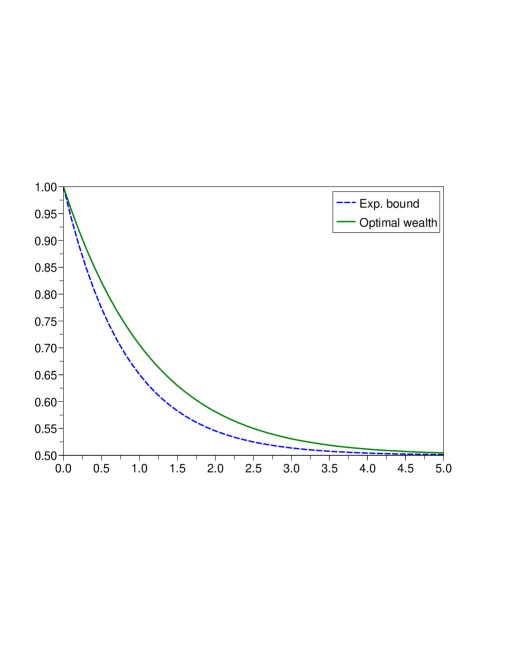
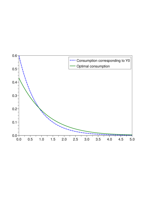
Figure 1: Left: typical profile of the optimal wealth process $Y_{t}$ and the exponential lower bound given by the proposition 5.8. Right: the corresponding consumption strategies. In the presence of investment opportunities, the agent first consumes slowly but if the investment opportunity does not appear, the agent eventually “gets disappointed” and starts to consume fast.

5.2.2 The nonstationary case

In this case the regularity results for the optimal strategies are weaker and more difficult to prove.

Proposition 5.9.

Let $a\in A$ and $(t,x)\in{\mathbb{R}}_{+}\times[l(a),+\infty)$. Let $(\bar{c}_{\cdot},\bar{Y}_{\cdot})$ be the optimal couple for the auxiliary problem starting at $(t,x)$. If $x=l(a)$, then $\bar{c}\equiv 0$, so $\bar{Y}\equiv l(a)$. If $x>l(a)$ then $\bar{c}$ is continuous, strictly positive and $\lim_{t\to+\infty}\bar{c}_{t}=0$.

Proof.

The proof is the same as in the stationary case. ∎

Note that, with respect to the stationary case here we do not have monotonicity of the optimal consumption since the behavior of $\hat{v}$ in the time variable is not known.

Moreover here the limiting property for $\bar{Y}$ is proved only under the assumption of twice continuous differentiability of $U$, as given below.

As in the stationary case we can deduce an autonomous equation for the optimal wealth process between two trading dates. However, since we have weaker regularity results the proof is different and makes use of the maximum principle.

Proposition 5.10.

Suppose that $U\in C^{2}((0,\infty))$ with $U^{\prime\prime}(x)<0$ for all $x$. Then the optimal wealth process $Y_{s}$ between two trading dates is twice differentiable, it satisfies the second-order ODE

$$\frac{\mathrm{d}^{2}Y_{s}}{\mathrm{d}s^{2}}=\frac{\frac{\partial g(s,Y_{s})}{\partial x}-(\rho+\lambda)U^{\prime}(c_{s})}{U^{\prime\prime}(c_{s})},\quad c_{s}=-\frac{\mathrm{d}Y_{s}}{\mathrm{d}s},\quad Y_{t}=x$$ (5.12)

and $\lim_{t\to+\infty}\bar{Y}_{t}=l(a)$.

Proof.

We cannot differentiate equations (2.12) and (5.1) with respect to $x$ as in the stationary case as we do not know if $\hat{v}$ is $C^{2}$. Then we follow a different approach. We use the maximum principle contained in Theorem 12 p 234 of [10]. Such theorem concerns problems with endpoint constraints but without state constraints. Due to the positivity of the consumption, our auxiliary problem (2.7) can be easily rephrased substituting the state constraint $Y_{s}\geq l(a),\forall s\geq t$ with the endpoint constraint $\lim_{s\to+\infty}Y_{s}\geq l(a)$. So we can apply the above quoted theorem that, applied to our case, states the following:

Assume that $g(\cdot,\cdot)$ and $\frac{\partial g(\cdot,\cdot)}{\partial x}$ are continuous. Given an optimal couple $(\bar{Y}_{\cdot},\bar{c}_{\cdot})$ with $\bar{c}$ continuous there exists a function $p(\cdot)\in C^{1}(t,+\infty;{\mathbb{R}})$ such that:

• $p(\cdot)$ is a solution of the equation

  $$p^{\prime}(s)=(\rho+\lambda)p(s)-\frac{\partial g(s,\bar{Y}_{s})}{\partial x};$$

• $U^{\prime}(\bar{c}_{s})=p(s)\;\leftrightarrow\;\bar{c}_{s}=I(p(s))$ for every $s\geq t$;

• $\lim_{T\to+\infty}e^{(\rho+\lambda)(s-T)}p(T)=0$, for every $t\leq s\leq T$ (transversality condition).

Since we already know (from Proposition 5.1) that there exists a unique optimal couple $(\bar{Y}_{\cdot},\bar{c}_{\cdot})$ and that $\bar{c}$ is continuous (see of Proposition 5.9) the above statements apply. Then we get that $\bar{c}_{s}>0$ for every $s\geq t$, that $\bar{c}$ is everywhere differentiable and that

$$\frac{\mathrm{d}\bar{c}_{s}}{\mathrm{d}s}=I^{\prime}(p(s))p^{\prime}(s)=\frac{1}{U^{\prime\prime}(\bar{c}_{s})}\left[(\rho+\lambda)U^{\prime}(\bar{c}_{s})-\frac{\partial g(s,\bar{Y}_{s})}{\partial x}\right]$$

which gives the claim recalling that $\bar{c}_{s}=-\displaystyle\frac{\mathrm{d}\bar{Y}_{s}}{\mathrm{d}s}$.

Concerning the limiting property of $\bar{Y}$ we argue by contradiction. Let $\lim_{s\to+\infty}\bar{Y}_{s}=x_{1}>l(a)$. We have then, by the definition of $g$, for every $s\geq t$,

$$\frac{\partial g(s,\bar{Y}_{s})}{\partial x}\leq\frac{\partial g(s,x_{1})}{\partial x}\leq\lambda v^{\prime}(x_{1}-l(a))<+\infty.$$

Then from the costate equation we get that, for $t\leq s\leq T<+\infty$

$$p(s)\leq e^{(\rho+\lambda)(s-T)}p(T)+\int_{s}^{T}e^{(\rho+\lambda)(r-T)}\lambda v^{\prime}(x_{1}-l(a))\mathrm{d}r$$

$$\leq e^{(\rho+\lambda)(s-T)}p(T)+\frac{\lambda}{\rho+\lambda}v^{\prime}(x_{1}-l(a))(1-e^{-(\rho+\lambda)T})$$

Using that $\lim_{T\to+\infty}e^{(\rho+\lambda)(s-T)}p(T)=0$ we get a uniform bound for $p(s)$. This is a contradiction as $\lim_{s\to+\infty}p(s)=\lim_{s\to+\infty}U^{\prime}(c_{s})=+\infty$. ∎

The equation (5.12) is a second-order ODE similar to equations of theoretical mechanics (second Newton’s law), and it should be solved on the interval $[0,+\infty)$ with the boundary conditions $Y_{0}=x$ and $Y_{\infty}=l(a)$ (which corresponds to resetting the time to zero after the last trading date). Solving this equation does not require the auxiliary value function $\hat{v}$ but only the original value function $v$, which, in the case of power utility, can be found from the scaling relation.

Remark 5.11.

The Maximum Principle used in the above proof holds once we know that $g(\cdot,\cdot)$ and $\frac{\partial g(\cdot,\cdot)}{\partial x}$ are continuous. As observed in Remark 4.12, this is true also in cases when the semiconcavity assumption 4.7 may fail (notably in the case of power utility and in the case of ‘regular’ density). So, also in such cases the Maximum Principle could be used to get information about the optimal strategies. Clearly, without knowing the regularity of the value function $\hat{v}$ such information would be much less satisfactory.

The case of power utility.

In the case of power utility function, the equation (5.12) can again be simplified:

$$\frac{\mathrm{d}^{2}Y_{t}}{\mathrm{d}t^{2}}=\frac{\rho+\lambda}{1-\gamma}c_{t}-\frac{\lambda\vartheta_{1}c^{2-\gamma}_{t}}{K_{1}(1-\gamma)}\int(Y_{t}+az)^{\gamma-1}p(t,\mathrm{d}z),\quad Y_{0}=x,\quad Y_{\infty}=l(a).$$

Because the second term in the right-hand side is still positive, the exponential bound of Proposition 5.8 can be established in exactly the same way as in the stationary case. Figure 2 depicts the optimal wealth process and the optimal consumption policy for the probability distribution $p(t,\mathrm{d}z)$ extracted from the Black-Scholes model with the same parameter values as in [5]: drift $b=0.4$, volatility $\sigma=1$, discount factor $\rho=0.2$, intensity $\lambda=2$ and risk aversion coefficient $\gamma=0.5$. We see that at least qualitatively, the consumption profile is similar to the one observed in the stationary model, with exponential decay. For comparison, we also plot the wealth and consumption policy for the stationary model with distribution corresponding to the Black-Scholes model in $3$ years’ time. In this case the agent consumes at a slower rate than in the nonstationary model. The explanation is that for the parameter values we chose, 3 years is a very long time horizon, because all the consumption happens, essentially, during the first 2 years after trading. During this period (first 2 years) the stationary model offers better investment opportunities, which explains the slower consumption rate.

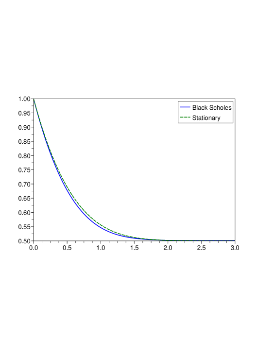
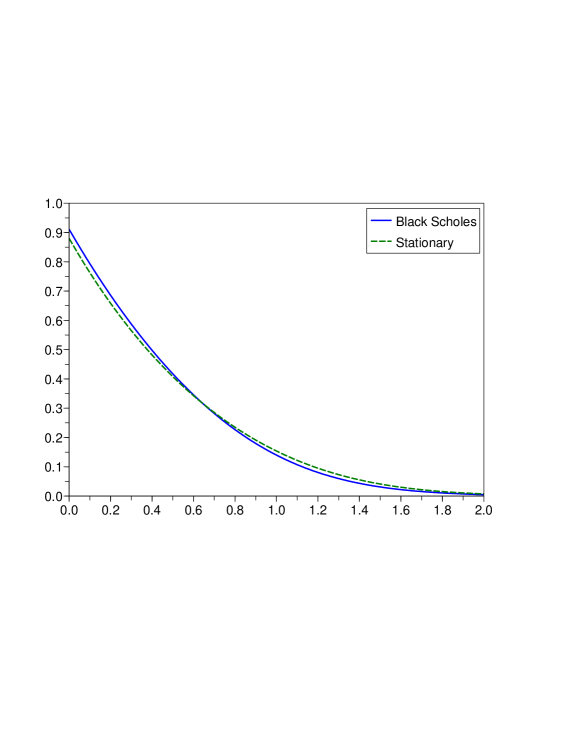
Figure 2: Optimal wealth (left) and consumption policy (right) for the probability distribution extracted from the Black-Scholes model (solid line) and from the stationary model having the same distribution as the Black-Scholes model in $3$ years’ time (dashed line).

Appendix A Appendix : Technical proofs

Proof of Proposition 3.1.

We suppose by contradiction that $v$ is not strictly increasing on ${\mathbb{R}}_{+}$ This means that it is definitely constant on ${\mathbb{R}}_{+}$ from a certain $x$ on, since $v$ is concave. Then we fix $\bar{x}\in{\mathbb{R}}_{+}$ such that $v(x)=B\in{\mathbb{R}}_{+}$, for all $x\geq\bar{x}$. Take $\epsilon>0$ and a pair $(\alpha^{\epsilon},c^{\epsilon})$ $\epsilon$-optimal at $\bar{x}$. This means that $(\alpha^{\epsilon},c^{\epsilon})\in{\mathcal{A}}(\bar{x})$, i.e.

$$X_{k}^{\bar{x}}=\bar{x}-\int_{0}^{\tau_{k}}c^{\epsilon}_{t}\mathrm{d}t+\sum_{i=1}^{k}\alpha^{\epsilon}_{i}Z_{i}\geq 0,\quad\forall k\geq 1,\quad X_{0}^{\bar{x}}=\bar{x},$$

and

$$B=v(\bar{x})<\mathbb{E}\left[\int_{0}^{+\infty}e^{-\rho t}U(c_{t}^{\epsilon})\mathrm{d}t\right]+\epsilon.$$

Now we choose $\tilde{x}>\bar{x}+1$. Then we have $v(\tilde{x})=v(\bar{x})=B$. We consider the control policy $(\alpha^{\epsilon},\tilde{c})$, where $\tilde{c}_{t}=c_{t}^{\epsilon}+\mathbb{I}_{[0,1]}(t)$, for all $t\geq 0$. Hence given $\tilde{x}>0$, we have for every $k\geq 1$,

$$X_{k}^{\tilde{x}} =\tilde{x}-\int_{0}^{\tau_{k}}\tilde{c}_{t}\mathrm{d}t+\sum_{i=1}^{k}\alpha^{\epsilon}_{i}Z_{i}=\tilde{x}-\int_{0}^{\tau_{k}}c_{t}^{\epsilon}\mathrm{d}t-(1\wedge\tau_{k})+\sum_{i=1}^{k}\alpha^{\epsilon}_{i}Z_{i}$$

$$>\bar{x}-\int_{0}^{\tau_{k}}c_{t}^{\epsilon}\mathrm{d}t+\sum_{i=1}^{k}\alpha^{\epsilon}_{i}Z_{i}\geq 0,$$

with $X_{0}^{\tilde{x}}=\tilde{x}$, so $(\alpha^{\epsilon},\tilde{c})\in{\mathcal{A}}(\tilde{x})$. Moreover we have:

$$v(\tilde{x})\geq\mathbb{E}\bigg{[}\int_{0}^{+\infty} e^{-\rho t}U(\tilde{c}_{t})\mathrm{d}t\bigg{]}=\mathbb{E}\left[\int_{0}^{1}e^{-\rho t}U(c_{t}^{\epsilon}+1)\mathrm{d}t\right]+\mathbb{E}\left[\int_{1}^{+\infty}e^{-\rho t}U(c_{t}^{\epsilon})\mathrm{d}t\right]$$

$$>\mathbb{E}\left[\int_{0}^{1}e^{-\rho t}U(c_{t}^{\epsilon})\mathrm{d}t\right]+\mathbb{E}\left[\int_{1}^{+\infty}e^{-\rho t}U(c_{t}^{\epsilon})\mathrm{d}t\right]=v(\bar{x})=B,$$

since $U$ is strictly increasing. But this is not possible, since we have assumed $v$ constant from $\bar{x}$ on. Hence the statement is proved.

$\square$

Proof of Proposition 3.2.

1. The continuity comes from condition d) of Assumption 2.2. If d) does not hold, measurability follows from condition b) of Assumption 2.2.

2. The function $g$ is strictly increasing in $x\in[l(a),+\infty)$ since $v$ is strictly increasing by Proposition 3.1.

3. This property is a direct consequence of concavity of $v$. Indeed, given $t\geq 0$, consider $(x_{\eta},a_{\eta})=(\eta x_{1}+(1-\eta)x_{2},\eta a_{1}+(1-\eta)a_{2})$, with $\eta\in(0,1)$, $x_{1}\geq l(a_{1}),x_{2}\geq l(a_{2})$. First of all, $x_{\eta}\geq l(a_{\eta})$ thanks to the convexity of the function $l$. Since $v$ is concave, we have for every $t\geq 0$:

   $$g(t,x_{\eta},a_{\eta}) =\lambda\int v\left(\eta x_{1}+(1-\eta)x_{2}+\eta a_{1}z+(1-\eta)a_{2}z\right)p(t,\mathrm{d}z)$$

   $$\geq\lambda\eta\int v\left(x_{1}+a_{1}z\right)p(t,\mathrm{d}z)+\lambda(1-\eta)\int v\left(x_{2}+a_{2}z\right)p(t,\mathrm{d}z)$$

   $$=\lambda\eta g(t,x_{1},a_{1})+\lambda(1-\eta)g(t,x_{2},a_{2}).$$

   This provides the result.

$\square$

Proof of Proposition 5.1.

In order to prove Proposition 5.1, we need the following preliminary result:

Lemma A.1.

Let $\hat{v}$ be the value function given in (2.7). Fix $a\in A$. Assume the followings:

• $\hat{v}(\cdot,\cdot,a)\in C^{1}\left({\mathbb{R}}_{+}\times(l(a),+\infty)\right)$;

• $\displaystyle\frac{\partial\hat{v}(t,l(a)^{+},a)}{\partial x}=+\infty$, for every $t\in{\mathbb{R}}_{+}$;

• $\hat{v}$ is a classical solution of the HJ equation (2.12) satisfying the growth condition (3.3) with representation (3.2) on the boundary.

Given $x\in[l(a),+\infty)$ and $t\geq 0$, for every couple $(c,Y)$ admissible at $(t,x)$ for $s\geq t$, we have the following identity: for $T>t$

$$\begin{split}&e^{-(\rho+\lambda)T}\hat{v}\left(T,Y_{T},a\right)-e^{-(\rho+\lambda)t}\hat{v}(t,x,a)=-\int_{t}^{T}e^{-(\rho+\lambda)s}\left[U(c_{s})+g(s,Y_{s},a)\right]\mathrm{d}s\\ &\quad\quad+\int_{t}^{T}e^{-(\rho+\lambda)s}\bigg{[}U(c_{s})-c_{s}\frac{\partial\hat{v}(s,Y_{s},a)}{\partial x}-\tilde{U}\left(\frac{\partial\hat{v}(s,Y_{s},a)}{\partial x}\right)\bigg{]}\mathrm{d}s,\end{split}$$ (A.1)

with the agreement that

$$\frac{\partial\hat{v}(t,l(a),a)}{\partial x}=\frac{\partial\hat{v}(t,l(a)^{+},a)}{\partial x}=+\infty,\ \mbox{so\ that}\ \tilde{U}\left(\frac{\partial\hat{v}(s,l(a),a)}{\partial x}\right)=0.$$

If $T$ goes to $+\infty$

$$\begin{split}&\hat{v}(t,x,a)=\int_{t}^{+\infty}e^{-(\rho+\lambda)(s-t)}\bigg{[}U(c_{s})+g(s,Y_{s},a)\bigg{]}\mathrm{d}s\\ &\quad-\int_{t}^{+\infty}e^{-(\rho+\lambda)(s-t)}\bigg{[}U(c_{s})-c_{s}\frac{\partial\hat{v}(s,Y_{s},a)}{\partial x}-\tilde{U}\left(\frac{\partial\hat{v}(s,Y_{s},a)}{\partial x}\right)\bigg{]}\mathrm{d}s.\end{split}$$ (A.2)

Furthermore, an admissible couple $(c,Y)$ is optimal at $(t,x)$ if and only if

$$\tilde{U}\bigg{(}\frac{\partial\hat{v}(s,Y_{s},a)}{\partial x}\bigg{)}=U(c_{s})-c_{s}\frac{\partial\hat{v}(s,Y_{s},a)}{\partial x},\quad{\rm for\ a.e.}\ s\geq t$$

such that $Y_{s}>l(a)$ and $c_{s}=0$ otherwise.

Proof.

Let $(c,Y)$ be an admissible couple for the auxiliary problem such that $Y_{s}>l(a)$, for every $s\geq t$. By applying standard differential calculus to $e^{-(\rho+\lambda)s}\hat{v}(s,Y_{s},a)$ between $s=t$ and $s=T$, we have:

$$e^{-(\rho+\lambda)T}\hat{v}(T,Y_{T},a)-e^{-(\rho+\lambda)t}\hat{v}(t,x,a)$$

$$\ =\int_{t}^{T}e^{-(\rho+\lambda)s}\left[\frac{\partial\hat{v}(s,Y_{s},a)}{\partial t}-(\rho+\lambda)\hat{v}(s,Y_{s},a)-c_{s}\frac{\partial\hat{v}(s,Y_{s},a)}{\partial x}\right]\mathrm{d}s$$

$$\quad=\int_{t}^{T}e^{-(\rho+\lambda)s}\left[-\tilde{U}\left(\frac{\partial\hat{v}(s,Y_{s},a)}{\partial x}\right)-g(s,Y_{s},a)-c_{s}\frac{\partial\hat{v}(s,Y_{s},a)}{\partial x}\right]\mathrm{d}s,$$

where in the last equation we have used the fact that $\hat{v}$ satisfies (2.12). This can be easily rewritten as (A.1) by adding and subtracting $U(c_{s})$ in the integrand. Now, from the growth condition (3.3) and since $\hat{v}$ is nondecreasing in $x$, we have

$$0\leq\hat{v}(T,Y_{T},a)\leq\hat{v}(T,x,a)\leq K(e^{bT}x)^{\gamma}\quad{\rm a.s.}$$

from which we deduce by Lemma 4.2 of [6] that

$$\lim_{T\to+\infty}e^{-(\rho+\lambda)T}\hat{v}\left(T,Y_{T},a\right)=0,\quad{\rm a.s.}$$

Hence, by sending $T$ to infinity, we can easily derive the relation (A.2). Let $(c,Y)$ be an admissible couple such that $Y_{T_{0}}=l(a)$, for a $T_{0}<+\infty$. Assume that $T_{0}$ is the first time when this happens. Then $Y_{s}=l(a)$, and $c_{s}=0$ for every $s\geq T_{0}$. Then for $T<T_{0}$ we get (A.1) as before. Calling

$$\begin{split}I_{T}:=-\int_{t}^{T}e^{-(\rho+\lambda)s}\left[U(c_{s})-c_{s}\frac{\partial\hat{v}(s,Y_{s},a)}{\partial x}-\tilde{U}\left(\frac{\partial\hat{v}(s,Y_{s},a)}{\partial x}\right)\right]\mathrm{d}s,\end{split}$$

we have that $I_{T}$ is increasing and from (A.1) that there exists its limit for $T\nearrow T_{0}$ given by:

$$-e^{-(\rho+\lambda)T_{0}}\hat{v}\left(T_{0},l(a),a\right)+e^{-(\rho+\lambda)t}\hat{v}(t,x,a)-\int_{t}^{T_{0}}e^{-(\rho+\lambda)(s-t)}\left[U(c_{s})+g(s,Y_{s},a)\right]\mathrm{d}s.$$

>From the positivity of the integrand in $I_{T}$, we then get that identity (A.1) also holds in $T_{0}$. For $T>T_{0}$ we can easily derive (A.1) using the fact that the couple $(c,Y)$ is constant after $T_{0}$ and that (ii) holds. Now, let us focus on the last statement. Let $(c,Y)$ be an admissible couple at $(t,x)$. Then $(c,Y)$ is optimal at $(t,x)$ if and only if in (A.2) we have

$$\hat{v}(t,x,a)=\int_{t}^{+\infty}e^{-(\rho+\lambda)(s-t)}\left[U(c_{s})+g(s,Y_{s},a)\right]\mathrm{d}s.$$

When $Y_{s}>l(a)$, for $s\geq t$, this is clearly equivalent to

$$\int_{t}^{+\infty}e^{-(\rho+\lambda)(s-t)}\left[U(c_{s})-c_{s}\frac{\partial\hat{v}(s,Y_{s},a)}{\partial x}-\tilde{U}\left(\frac{\partial\hat{v}(s,Y_{s},a)}{\partial x}\right)\right]\mathrm{d}s=0,$$

i.e.

$$\tilde{U}\left(\frac{\partial\hat{v}(s,Y_{s},a)}{\partial x}\right)=U(c_{s})-c_{s}\frac{\partial\hat{v}(s,Y_{s},a)}{\partial x},\quad{\rm for}\ {\rm a.e.}\ s\geq t.$$ (A.3)

When $Y_{s}>l(a)$ on $(t,T)$, we have (A.3) on $(t,T)$ and $c_{s}=0$ on $[T,+\infty)$. ∎

Now we come to the proof of the Proposition 5.1. First we observe that, thanks to Proposition 4.9 the assumptions (i)-(ii)-(iii) of the previous Lemma A.1 hold. So fix $(t,x,a)\in{\mathcal{D}}$. First we prove the existence of a solution $\bar{Y}$ of the problem (5.3). The dynamics of the system is the function $-\hat{c}(\cdot,\cdot,a):{\mathbb{R}}_{+}\times(l(a),+\infty)\to(0,+\infty)$, with (5.1), that is well-defined and continuous as composition of continuous functions on ${\mathbb{R}}_{+}\times(l(a),+\infty)$. We note that hypothesis (ii) of Lemma A.1 implies $\hat{c}(t,l(a)^{+},a)=0$, for every $t\geq 0$. Hence, we can extend the function $\hat{c}(\cdot,\cdot,a)$ to a continuous function on ${\mathbb{R}}_{+}\times(-\infty,+\infty)$ such that $\hat{c}=0$ on ${\mathbb{R}}_{+}\times(-\infty,l(a)]$. Now the Peano’s Theorem guarantees the existence of a local solution $\bar{Y}_{\cdot}$ of (5.3). We prove that $(s,\bar{Y}_{s},a)\in{\mathcal{D}}$ for every $s\geq t$, i.e. that

$$\bar{Y}_{s}\geq l(a),\quad\mbox{for}\ s\geq t.$$ (A.4)

If $x=l(a)$, we already know that $\hat{c}(s,l(a)^{+},a)=0$, for $s\geq t$, given $t$, so that $\bar{Y}_{s}=l(a)$, for all $s\geq t$.
Now we suppose $x>l(a)$. Since $-\hat{c}(s,y,a)<0$, for each $(s,y)\in[t,+\infty)\times(l(a),+\infty)$, the solution $\bar{Y}$ is strictly decreasing on the maximal interval that we denote by $(t,T)$, with $T>0$. Suppose that there exists an instant $t<t^{\prime}<T$ such that $\bar{Y}_{t^{\prime}}<l(a)$. We have that $\mathrm{d}\bar{Y}_{t^{\prime}}=0$. In particular this means that there exists an interval $[t_{0},t_{1}]\subset(t,T)$ with $\bar{Y}_{t_{0}}=l(a)$ and $\bar{Y}_{t_{1}}<l(a)$ such that for all $s\in(t_{0},t_{1}]$, $\hat{Y}_{s}<l(a)$ with $\mathrm{d}\bar{Y}_{s}(t,x,a)=0$, that it is not possible. This proves the claim (A.4), for any $x\geq l(a)$ and that $T=+\infty$.
Now call $\bar{c}_{s}=\hat{c}(s,\bar{Y}_{s},a)$ as in (5.2). Then the couple $(\bar{c},\bar{Y})$ is admissible since $\bar{c}_{s}\geq 0$, for every $s\geq t$ and $\bar{Y}_{s}\geq l(a)$, for $s\geq t$. Moreover

$$\tilde{U}\left(\frac{\partial\hat{v}}{\partial x}(s,\bar{Y}_{s},a)\right)=U(c_{s})-\bar{c}_{s}\frac{\partial\hat{v}}{\partial x}(s,\bar{Y}_{s},a),\quad\mbox{for}\ {\rm a.e.}\ s\geq t,$$

so the couple $(\bar{c},\bar{Y})$ is optimal at $(t,x)$ thanks to Lemma A.1. Hence the existence of an optimal couple for the auxiliary problem is proved.
Now we prove the uniqueness. Fix $a\in{\mathcal{A}}$, $x\geq l(a)$ and $t\geq 0$. Let $\bar{c}_{1}$, $\bar{c}_{2}$ be optimal controls at $x$. Then for $i=1,2$

$$\hat{v}(t,x,a) =\int_{t}^{+\infty}e^{-(\rho+\lambda)(s-t)}\left[U(\bar{c}_{i}(s))+g(s,\bar{Y}_{s}^{t,x}(\bar{c}_{i}),a)\right]\mathrm{d}s$$

$$=\int_{0}^{+\infty}e^{-(\rho+\lambda)s}\left[U(\bar{c}_{i}(s))+g(s+t,\bar{Y}_{s}^{x}(\bar{c}_{i}),a)\right]\mathrm{d}s,$$

where for every $c\in{\mathcal{C}}_{a}(x)$, $Y_{s}^{x}(c)=x-\int_{0}^{s}c(u)\mathrm{d}u,\ s\geq 0$. Since the function $U$ is strictly concave, we have by setting $c_{\eta}=\eta\bar{c}_{1}+(1-\eta)\bar{c}_{2}$, with $\eta\in(0,1)$,

$$U(c_{\eta}(s))=U\left(\eta\bar{c}_{1}(s)+(1-\eta)\bar{c}_{2}(s)\right)>\eta_{1}U(\bar{c}_{1}(s))+(1-\eta)U(\bar{c}_{1}(s)),\quad s\geq 0.$$

Moreover, since $\bar{Y}_{s}^{x}(c_{\eta})=\eta\bar{Y}_{s}^{x}(\bar{c}_{1})+(1-\eta)\bar{Y}_{s}^{x}(\bar{c}_{2})$, for all $s\geq 0$ and $g$ is concave in the second variable, we have

$$g(s+t,\bar{Y}_{s}^{x}(c_{\eta}),a)\geq\eta g(s+t,\bar{Y}_{s}^{x}(\bar{c}_{1}),a)+(1-\eta)g(s+t,\bar{Y}_{s}^{x}(\bar{c}_{2}),a),\quad\forall s\geq 0.$$

Then

$$\hat{v}(t,x,a)<\int_{0}^{+\infty}e^{-(\rho+\lambda)s}\left[U(c_{\eta}(s))+g(s+t,\bar{Y}_{s}^{x}(c_{\eta}),a)\right]\mathrm{d}s,$$

that implies the uniqueness of the control of the auxiliary problem.

$\square$

References

• [1] Bardi M. and Capuzzo-Dolcetta I. (1997), Optimal Control and Viscosity Solutions of Hamilton-Jacobi-Bellman Equations. Birkhäuser Boston Inc., Boston, MA.
• [2] Cannarsa P. and Sinestrari C. (2004), Semiconcave Functions, Hamilton-Jacobi Equations and Optimal Control. Progress in Nonlinear Differential Equations and their Applications, 58. Birkhäuser Boston Inc., Boston, MA.
• [3] Cannarsa P. and Soner H.M. (1989) “Generalized one-sided estimates for solutions of Hamilton-Jacobi equations and applications”, Nonlinear Analysis 13 (3), 305-323.
• [4] Matsumoto K. (2006) : “Optimal portfolio of low liquid assets with a log-utility function”, Finance and Stochastics, 10 (1), 121-145.
• [5] Pham H. and Tankov P. (2007), “A Model of Optimal Consumption under Liquidity Risk with Random Trading Times”. To appear in Mathematical Finance.
• [6] Pham H. and Tankov P. (2007), “A Coupled System of Integrodifferential Equations Arising in Liquidity Risk Model”. To appear in Applied Mathematics and Optimization.
• [7] Rockafellar R.T. (1970), Convex Analysis. Princeton University Press, Princeton.
• [8] Rogers C. (2001), “The relaxed investor and parameter uncertainty”, Finance and Stochastics, 5 (2), 131-154.
• [9] Rogers C. and Zane O. (2002) : “A simple model of liquidity effects”, in Advances in Finance and Stochastics: Essays in Honour of Dieter Sondermann, eds. K. Sandmann and P. Schoenbucher, 161–176.
• [10] Seierstad A. and Sydsaeter K. (1987), Optimal Control Theory with Economic Applications. North Holland, Amsterdam.