Large non-Gaussianity from multi-brid inflation

Abstract

A model of multi-component hybrid inflation, dubbed multi-brid inflation, in which various observable quantities including the non-Gaussianity parameter $f_{NL}$ can be analytically calculated was proposed recently. In particular, for a two-brid inflation model with an exponential potential and the condition that the end of inflation is an ellipse in the field space, it was found that, while keeping the other observational quantities within the range consistent with observations, large non-Gaussianity is possible for certain inflationary trajectories, provided that the ratio of the two masses is large. One might question whether the resulting large non-Gaussianity is specific to this particular form of the potential and the condition for the end of inflation. In this paper, we consider a model of multi-brid inflation with a potential given by an exponential function of terms quadratic in the scalar field components. We also consider a more general class of ellipses for the end of inflation than those studied previously. Then, focusing on the case of two-brid inflation, we find that large non-Gaussianity is possible in the present model even for the equal-mass case. Then by tuning the model parameters, we find that there exist models for which both the non-Gaussianity and the tensor-to-scalar ratio are large enough to be detected in the very near future.

I Introduction

The primordial non-Gaussianity has been one of the hottest topics in cosmology in recent years. The conventional, single-field slow-roll inflation predicts that the curvature perturbation is Gaussian to an extremely high accuracy Salopek:1990jq . In other words, if any primordial non-Gaussianity is detected, it strongly indicates that the dynamics of inflation is not as simple as we thought it to be.

The primordial non-Gaussianity is conveniently represented by a parameter denoted by $f_{NL}$ Komatsu:2001rj . Roughly, it is the ratio of the 3-point correlation function (or the bispectrum) to the square of the 2-point correlation function (or the square of the spectrum). It is expected that near-future experiments such as those of PLANCK will be able to detect $f_{NL}$ at a level as small as 5 Babich:2004yc .

Finding even a small deviation from Gaussianity will have profound implications on the theory of the early universe. Consequently, numerous types of inflationary models that produce detectable non-Gaussianity have been proposed and studied NGmodels1 ; NGmodels2 ; Bernardeau:2002jf ; Dvali:2003em ; Kofman:2003nx ; Lyth:2005qk ; Alabidi ; BarnabyCline ; Chambers:2007se . In terms of the nature of non-Gaussianities, most of these models can be classified into two categories; those with non-Gaussianities arising intrinsically from the quantum fluctuations, and those with non-Gaussianities due to nontrivial classical dynamics on superhorizon scales. A typical example of the former is the DBI inflation, in which the slow-roll condition can be fully violated Silverstein:2003hf . In this case, the equilateral $f_{NL}$ (denoted by $f_{NL}^{\rm equil}$) representing the amplitude of the bispectrum of the equilateral configurations, is found to play an important role DBIinflation . On the other hand, in the latter case where non-Gaussianities are produced on superhorizon scales, by causality the local $f_{NL}$ (denoted by $f_{NL}^{\rm local}$) characterizes the level of the non-Gaussianity. It is defined in terms of the coefficient in front of the second order curvature perturbation Komatsu:2001rj ,

$$\Phi=\Phi_{L}+f_{NL}^{\rm local}\Phi_{L}^{2}\,,$$ (1)

where $\Phi$ is the curvature perturbation on the Newtonian slice and $\Phi_{L}$ is its linear, Gaussian part.

In this paper, we focus on the latter case, that is, we consider models that may produce a large value of $f_{NL}^{\rm local}$, for example 10–100. More specifically, we consider hybrid inflation with multiple inflaton fields, dubbed multi-brid inflation Sasaki:2008uc . The inflaton fields are assumed to follow the slow-roll equations of motion, and their fluctuations are assumed to be Gaussian. In this case, the $\delta N$ formalism is most useful for the evaluation of the curvature perturbation and non-Gaussianity Sasaki:1995aw ; Sasaki:1998ug ; Wands:2000dp ; Lyth:2004gb ; Lyth:2005fi .

As in the conventional hybrid inflation, the inflaton fields are coupled to a water-fall field, and inflation ends when the inflaton fields satisfy a certain condition that triggers the instability of the water-fall field. However, unlike the case of a single inflaton field in which there is essentially no degree of freedom in the condition for the end of inflation, there is a substantial increase in the degree of freedom at the end of inflation in multi-brid inflation and it widens the viable range of the parameter space considerably and leads to the possibility of generating large non-Gaussianity.

As a model of multi-brid inflation, an analytically solvable two-brid inflation model was recently investigated in detail Sasaki:2008uc , where the potential was assumed to be exponential with the exponent given by a linear combination of the inflaton fields. In this paper, we consider a two-brid model with again an exponential potential but with the exponent given by a quadratic function of the inflaton fields. The potential has point symmetry about the origin of the field space, in contrast to the case of the linear exponent which has no symmetry. Thus by investigating the quadratic case, we will be able to see if the generation of large non-Gaussianity is a generic feature of multi-brid inflation or if it is due to the lack of symmetry that leads to large non-Gaussianity in the linear exponent case.

In passing, we mention that the possibility of large non-Gaussianity from loop correction terms in the perturbative expansion has recently been discussed by Cogollo et al. Cogollo:2008bi . Although such a case certainly needs further investigation, in this paper we concentrate on the case in which leading order (tree) terms dominate over loop correction terms.

This paper is organized as follows. In §2, we describe our model and derive basic formulas to be used in the proceeding sections. In §3, using the formulas derived in §2, we analytically compute the spectrum of the curvature perturbation ${\cal P}_{S}(k)$, its spectral index $n_{S}$, the tensor-to-scalar ratio $r$, and the non-Gaussianity parameter $f_{NL}^{\rm local}$. In §4, as a couple of special cases of our model, we analyze in detail the equal-mass case as well as the case of large mass ratio. We find that a large $f_{NL}^{\rm local}$ is possible in both cases. In particular, in the equal-mass case, by tuning the parameters to some extent, we find that it is possible to have both $r$ and $f_{NL}^{\rm local}$ large enough to be detected. We conclude the paper in §5. Some computational details are described in Appendix A. For comparison, we also summarize the result for the case of the linear exponent two-brid model in Appendix B. We use the Planck units where $M_{pl}^{-2}=8\pi G=1$.

II Two-brid inflation with approximately quadratic potential

We consider a two-component scalar field whose action is given by

$$S=-\int d^{4}x\sqrt{-g}\left[\frac{1}{2}g^{\mu\nu}\sum_{A=1,2}\partial_{\mu}\phi_{A}\partial_{\nu}\phi_{A}+V(\phi)\right]\,,$$ (2)

where the potential is given by

$$V=V_{0}(\chi,\phi_{1},\phi_{2})\exp\left[\frac{1}{2}\left(m_{1}^{2}\phi_{1}^{2}+m_{2}^{2}\phi_{2}^{2}\right)\right]\,,$$ (3)

with $V_{0}$ being a function of a water-fall field $\chi$ as well as of $\phi_{1}$ and $\phi_{2}$, but is assumed to be constant in time during inflation; see Eq. (13) below. The same model was previously analyzed Sasaki:2007ay . However, the condition for the end of inflation considered then was not general enough to allow the possibility of large non-Gaussianity.

The Friedmann and the field equations are

$$3H^{2}=\frac{1}{2}(\dot{\phi}_{1}^{2}+\dot{\phi}_{2}^{2})+V(\phi)\,,$$ (4)

$$\ddot{\phi}_{A}+3H\dot{\phi}_{A}+\frac{\partial V}{\partial\phi_{A}}=0\,,$$ (5)

where $H=\dot{a}/a$ and the dot $\dot{~{}}$ denotes a derivative with respect to the cosmic proper time; $\dot{~{}}=d/dt$. The slow-roll equations of motion are obtained by neglecting the kinetic term in the Friedmann equation and the second time derivative in the field equations. Thus the slow-roll equations of motion are

$$3H^{2}=V\,,\quad\frac{d\phi_{A}}{dN}=\frac{1}{V}\frac{\partial V}{\partial\phi_{A}}=m_{A}^{2}\phi_{A}\,,$$ (6)

where the number of $e$-folds counted backwards in time, $dN=-Hdt$, is used as the time variable for later convenience. Note that the effective mass squared $M_{A}^{2}$ for each $\phi_{A}$ is given by

$$M_{A}^{2}=\frac{\partial^{2}V}{\partial\phi_{A}^{2}}=m_{A}^{2}(1+m_{A}^{2}\phi_{A}^{2})V=3m_{A}^{2}(1+m_{A}^{2}\phi_{A}^{2})H^{2}\,.$$ (7)

Thus, the slow-roll condition is satisfied if $m_{A}^{2}\ll 1$ and $\phi_{A}^{2}$ are not too much larger than unity. Incidentally, since $m_{A}^{2}\phi_{A}^{2}\ll 1$ under this assumption, the difference between the present potential and a pure quadratic potential,

$$V=V_{0}+\frac{1}{2}(M_{1}^{2}\phi_{1}^{2}+M_{2}^{2}\phi_{2}^{2})\,,$$ (8)

is almost negligibly small (that is, they are equivalent to the leading order in the slow-roll approximation). An analytical solution for this separable potential model was first discussed by Starobinsky Starobinsky:1986fxa .

Introducing new field variables $q_{A}$ as

$$\ln q_{1}=\ln(q\cos\theta)=\int\frac{d\phi_{1}}{m_{1}^{2}\phi_{1}}=\frac{\ln\phi_{1}}{m_{1}^{2}}\,,\quad\ln q_{2}=\ln(q\sin\theta)=\frac{\ln\phi_{2}}{m_{2}^{2}}\,,$$ (9)

the slow-roll equations become

$$\frac{d\ln q}{dN}=1\,,\quad\frac{d\theta}{dN}=0\,.$$ (10)

Hence we immediately obtain

$$N=\ln q-\ln q_{f}=\frac{1}{2}\ln\left[\phi_{1}^{2/m_{1}^{2}}+\phi_{2}^{2/m_{2}^{2}}\right]-\frac{1}{2}\ln\left[\phi_{1,f}^{2/m_{1}^{2}}+\phi_{2,f}^{2/m_{2}^{2}}\right]\,,$$ (11)

where the number of $e$-folds is set to zero at the end of inflation and $\phi_{A,f}$ is the final value of the inflaton fields.

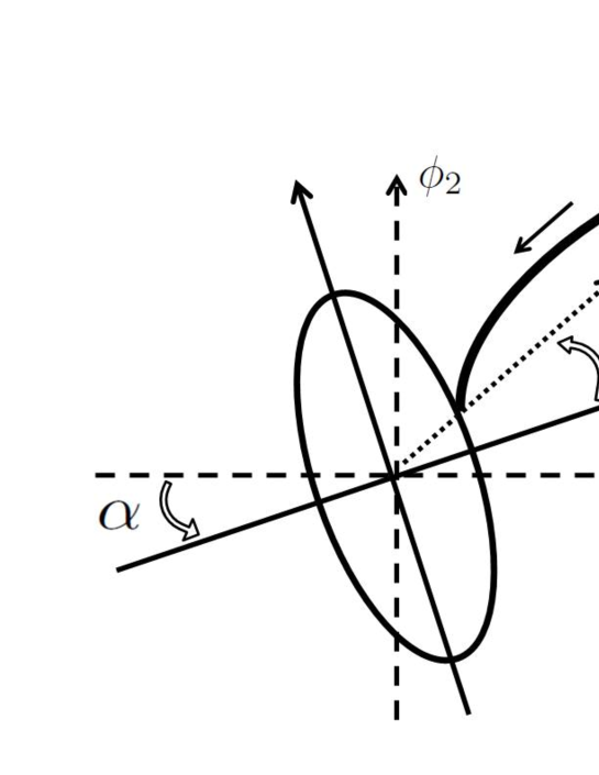
Figure 1: Definitions of parameters $\alpha$ and $\gamma$ in field space. The ellipse represents the surface of the end of inflation.

We assume that inflation ends at

$$\sigma^{2}=G(\phi_{1},\phi_{2})\equiv g_{1}^{2}(\phi_{1}\cos\alpha+\phi_{2}\sin\alpha)^{2}+g_{2}^{2}(-\phi_{1}\sin\alpha+\phi_{2}\cos\alpha)^{2}\,,$$ (12)

which is realized by the potential $V_{0}$ given by

$$V_{0}=\frac{1}{2}G(\phi_{1},\phi_{2})\chi^{2}+\frac{\lambda}{4}\left(\chi^{2}-\frac{\sigma^{2}}{\lambda}\right)^{2}.$$ (13)

We parametrize the scalar fields at the end of inflation as

$$\frac{\sigma}{g_{1}}\cos\gamma=\phi_{1,f}\cos\alpha+\phi_{2,f}\sin\alpha\,,\quad\frac{\sigma}{g_{2}}\sin\gamma=-\phi_{1,f}\sin\alpha+\phi_{2,f}\cos\alpha\,,$$ (14)

namely,

$$\phi_{1,f}=\frac{\sigma}{g_{1}g_{2}}(g_{2}\cos\alpha\cos\gamma-g_{1}\sin\alpha\sin\gamma),\quad\phi_{2,f}=\frac{\sigma}{g_{1}g_{2}}(g_{2}\sin\alpha\cos\gamma+g_{1}\cos\alpha\sin\gamma).$$ (15)

Figure 1 shows the definitions of the angles $\alpha$ and $\gamma$. The ellipse describes the surface at the end of inflation, defined by Eq. (12). The angle $\alpha$ describes the amount of rotation of the ellipse relative to the $\phi_{1}$ and $\phi_{2}$ axes. The angle $\gamma$ describes the position of the inflaton trajectory at the end of inflation.

Since $\theta$ is a constant of motion, we have

$$\ln\left[\frac{q_{1}}{q_{2}}\right] = \frac{1}{m_{1}^{2}}\ln\phi_{1}-\frac{1}{m_{2}^{2}}\ln\phi_{2}$$ (16)

$$= \frac{1}{m_{1}^{2}}\ln\frac{\sigma}{g_{1}g_{2}}(g_{2}\cos\alpha\cos\gamma-g_{1}\sin\alpha\sin\gamma)-\frac{1}{m_{2}^{2}}\ln\frac{\sigma}{g_{1}g_{2}}(g_{2}\sin\alpha\cos\gamma-g_{1}\cos\alpha\sin\gamma).$$ (17)

This equation determines the parameter $\gamma$ in terms of $\phi_{1}$ and $\phi_{2}$: $\gamma=\gamma(\phi_{1},\phi_{2})$. Hence, from Eq. (15), $\phi_{1,f}$ and $\phi_{2,f}$ become functions of $\phi_{1}$ and $\phi_{2}$,

$$\phi_{1,f}=\phi_{1,f}(\phi_{1},\phi_{2})\,,\quad\phi_{2,f}=\phi_{2,f}(\phi_{1},\phi_{2})\,.$$ (18)

With this understanding, the number of $e$-folds given by Eq. (11) becomes a function of $(\phi_{1},\phi_{2})$. It is then straightforward to obtain $\delta N$ to full nonlinear order. It can be straightforwardly calculated as

$$\delta N=N(\phi_{1}+\delta\phi_{1},\phi_{2}+\delta\phi_{2})-N(\phi_{1},\phi_{2})\,.$$ (19)

Before closing this section, let us make a small comment. As mentioned in Sasaki:2008uc , the above formula for $\delta N$ neglects the fact that the surface at the end of inflation, determined by Eq. (12), is not an equipotential surface. This will give rise to an additional correction to the final $\delta N$. Nevertheless, it turns out that the correction is small and can be neglected, as discussed in Sasaki:2008uc .

III Curvature perturbation and non-Gaussianity

In this section, we compute the curvature perturbation of our model explicitly, and evaluate the curvature perturbation spectrum ${\cal P}_{S}$, the spectral index $n_{S}$, the tensor-to-scalar ratio $r$, and the non-Gaussianity parameter $f_{NL}^{\rm local}$.

We expand the $\delta N$ formula Eq. (19) to the second order in $\delta\phi$ for $N(\phi_{1},\phi_{2})$ given in Eq. (11). Note that $\delta\gamma$ must be expressed in terms of $\delta\phi$ with second-order accuracy. Details are deferred to Appendix A. The result is

$$\delta N = \frac{\displaystyle-\frac{W}{Z}\frac{\delta\phi_{1}}{\phi_{1}}+\frac{Y}{X}\frac{\displaystyle\delta\phi_{2}}{\phi_{2}}}{\displaystyle m_{2}^{2}\frac{Y}{X}-m_{1}^{2}\frac{W}{Z}}$$ (22)

$$+\frac{1}{2}\frac{\displaystyle\frac{W}{Z}\left(\frac{\delta\phi_{1}}{\phi_{1}}\right)^{2}-\frac{Y}{X}\left(\frac{\delta\phi_{2}}{\phi_{2}}\right)^{2}}{\displaystyle m_{2}^{2}\frac{Y}{X}-m_{1}^{2}\frac{W}{Z}}-\frac{1}{2}\frac{\displaystyle\left(1-\frac{Y}{X}\frac{W}{Z}\right)\left(\displaystyle\frac{W}{Z}-\frac{Y}{X}\right)\left(\frac{\displaystyle m_{2}^{2}}{\phi_{1}}\delta\phi_{1}-\frac{\displaystyle m_{1}^{2}}{\phi_{2}}\delta\phi_{2}\right)^{2}}{\left(\displaystyle m_{2}^{2}\frac{Y}{X}-m_{1}^{2}\frac{W}{Z}\right)^{3}}+\cdots\,,$$

where we have introduced the quantities and defined as

$$g=\sqrt{g_{1}^{2}+g_{2}^{2}}\,,\quad g_{1}=g\cos\beta\,,\quad g_{2}=g\sin\beta\,,$$

$$X=\frac{1}{g}(g_{2}\cos\alpha\cos\gamma-g_{1}\sin\alpha\sin\gamma)\propto\phi_{1,f}\,,\quad Y=\frac{1}{g}(g_{2}\cos\alpha\sin\gamma+g_{1}\sin\alpha\cos\gamma)=-\frac{\partial}{\partial\gamma}X\,,$$

$$Z=\frac{1}{g}(g_{2}\sin\alpha\cos\gamma+g_{1}\cos\alpha\sin\gamma)\propto\phi_{2,f}\,,\quad W=\frac{1}{g}(g_{2}\sin\alpha\sin\gamma-g_{1}\cos\alpha\cos\gamma)=-\frac{\partial}{\partial\gamma}Z\,.$$

We note that $\tan\beta=g_{2}/g_{1}$. For example, in the case of Fig. 1, $\tan\beta$ is the ratio of the semiminor axis to the semimajor axis (hence $\beta<\pi/4$).

We assume that the scalar field fluctuations $\delta\phi_{1}$ and $\delta\phi_{2}$ are Gaussian with the dispersion,

$$\left\langle\delta\phi_{A}\delta\phi_{B}\right\rangle_{k}=\left(\frac{H}{2\pi}\right)^{2}_{t_{k}}\delta_{AB}\,,$$ (23)

where $t_{k}$ is the horizon-crossing time of the comoving wave number $k$, where $k=Ha$. Then the curvature perturbation spectrum is given by

$${\cal P}_{S}(k)\equiv\frac{4\pi k^{3}}{(2\pi)^{3}}P_{\cal{R}}(k)=\frac{g^{2}}{\sigma^{2}}\frac{\sin^{2}\beta\cos^{2}\beta}{(m_{2}^{2}\,YZ-m_{1}^{2}\,XW)^{2}}\left(W^{2}e^{-2m_{1}^{2}N_{k}}+Y^{2}e^{-2m_{2}^{2}N_{k}}\right)\left(\frac{H}{2\pi}\right)^{2}_{t_{k}}\,,$$ (24)

where $N_{k}$ is the number of $e$-folds at the horizon crossing, $N_{k}=N(t_{k})$. Using the fact that $3H^{2}=V$, the spectral index is found to be

$$n_{S}-1=2\frac{m_{1}^{2}e^{-2m_{1}^{2}N_{k}}W^{2}+m_{2}^{2}e^{-2m_{2}^{2}N_{k}}Y^{2}}{e^{-2m_{1}^{2}N_{k}}W^{2}+e^{-2m_{2}^{2}N_{k}}Y^{2}}-\frac{\sigma^{2}}{g^{2}}\frac{m_{1}^{4}e^{2m_{1}^{2}N_{k}}X^{2}+m_{2}^{4}e^{2m_{2}^{2}N_{k}}Z^{2}}{\sin^{2}\beta\cos^{2}\beta}\,.$$ (25)

The tensor-to-scalar ratio is given by

$$r\equiv\frac{{\cal P}_{T}}{{\cal P}_{S}}=8\frac{\sigma^{2}}{g^{2}}\frac{(m_{2}^{2}YZ-m_{1}^{2}XW)^{2}}{\sin^{2}\beta\cos^{2}\beta}\frac{1}{W^{2}e^{-2m_{1}^{2}N_{k}}+Y^{2}e^{-2m_{2}^{2}N_{k}}}\,.$$ (26)

Now we evaluate the non-Gaussianity in our model. For convenience, we introduce the linear curvature perturbation ${\cal R}_{L}$ and the linear entropy perturbation $S$,

$${\cal R}_{L}=\frac{\displaystyle-\frac{XW}{\phi_{1}}\delta\phi_{1}+\frac{YZ}{\phi_{2}}\delta\phi_{2}}{m_{2}^{2}\,YZ-m_{1}^{2}\,XW}\,,\quad S=\frac{\displaystyle\frac{YZ}{\phi_{2}}\delta\phi_{1}+\frac{XW}{\phi_{1}}\delta\phi_{2}}{m_{2}^{2}\,YZ-m_{1}^{2}\,XW}\,.$$ (27)

For the Gaussian fluctuations $\delta\phi_{A}$ given by Eq. (23), we see that $S$ has the same spectrum as the curvature perturbation ${\cal R}_{L}$, but is orthogonal to it,

$$\left\langle{\cal R}_{L}\cdot S\right\rangle=0\,.$$ (28)

In terms of ${\cal R}_{L}$ and $S$, the nonlinear $\delta N$ in Eq. (22) is re-expressed as

$$\delta N={\cal R}_{L}+\frac{3}{5}f_{NL}^{\rm local}\,{\cal R}_{L}^{2}+C_{RS}\,{\cal R}_{L}\,S+C_{SS}\,S^{2}+\cdots\,,$$ (29)

where the non-Gaussian parameter $f_{NL}^{\rm local}$ is given by

$$f_{NL}^{\rm local}=XZ$$ (30)

(31)

$$~{}\times\frac{5}{6}\frac{\left(\displaystyle\frac{W^{3}}{X}e^{4m_{2}^{2}N_{k}}-\frac{Y^{3}}{Z}e^{4m_{1}^{2}N_{k}}\right)\left(\displaystyle m_{2}^{2}\frac{Y}{X}-m_{1}^{2}\frac{W}{Z}\right)^{2}-\left(XZ-YW\right)\left(\displaystyle\frac{W}{Z}-\frac{Y}{X}\right)\left(\displaystyle m_{1}^{2}\frac{Y}{Z}e^{2m_{1}^{2}N_{k}}+m_{2}^{2}\frac{W}{X}e^{2m_{2}^{2}N_{k}}\right)^{2}}{\left(\displaystyle m_{2}^{2}\frac{Y}{X}-m_{1}^{2}\frac{W}{Z}\right)\left(Y^{2}e^{2m_{1}^{2}N_{k}}+W^{2}e^{2m_{2}^{2}N_{k}}\right)^{2}}\,.$$ (32)

(33)

This is one of our main results.

Before closing this section, let us briefly discuss the non-Gaussianity due to the other second order coefficients $C_{RS}$ and $C_{SS}$. Although the derivation of their expressions is straightforward, we do not present their explicit expressions here, because they are as complicated as Eq. (33) and because they are unnecessary for the purpose of the present paper. We only mention that an inspection of the resulting expressions reveals that they can never become much larger than $f_{NL}^{\rm local}$. To be a bit more precise, their values can become large for certain ranges of the parameters, but when they become large, $f_{NL}^{\rm local}$ also becomes large simultaneously. Hence, as discussed in Sasaki:2008uc , as long as we focus on the bispectrum, we can neglect their contribution.

IV Case for large non-Gaussianity

Since Eq. (33) for $f_{NL}^{\rm local}$ is very complicated, it is not easy to study all possible cases in detail. However, there are some limiting cases in which we have a substantially simplified expression for $f_{NL}^{\rm local}$ but which are yet sufficiently of interest.

One case of interest is when the two masses are equal, $m_{1}=m_{2}$. In this case, the potential during inflation is O(2) symmetric. This symmetry is broken at the end of inflation because of condition (12), unless $g_{1}=g_{2}$. This model was discussed by Alabidi and Lyth Alabidi as a new mechanism of generating curvature perturbations. Another case of interest is when the ratio of the mass parameters are large, for example, $m_{1}\gg m_{2}$. In this large mass ratio limit, an inspection of the Eq. (33) suggests that a large value of $f_{NL}^{\rm local}$ may be possible if the parameter $W$ is very small. In this section, we investigate these two cases in detail.

IV.1 Equal mass

First let us consider the equal mass case, $m_{1}^{2}=m_{2}^{2}\equiv m^{2}$. This means that there is O(2) symmetry during inflation, and the symmetry is spontaneously broken at the end of inflation Alabidi .

In the equal-mass case, the formulas derived in the previous section simplify considerably to

$${\cal{P}}_{S} = \left(\frac{g}{\sigma m^{2}e^{m^{2}N_{k}}}\right)^{2}\frac{1+\cos 2\beta\cos 2\gamma}{2}\left(\frac{H}{2\pi}\right)^{2}_{t_{k}}=\frac{8}{r}\left(\frac{H}{2\pi}\right)^{2}_{t_{k}}\,,$$ (34)

$$n_{S}-1 = 2m^{2}-2\left(\frac{\sigma m^{2}e^{m^{2}N_{k}}}{g}\right)^{2}\frac{1-\cos 2\beta\cos 2\gamma}{\sin^{2}2\beta}=2m^{2}-\frac{r}{8}\,\frac{1-\cos^{2}2\beta\cos^{2}2\gamma}{\sin^{2}2\beta}\,,$$ (35)

$$r = 8\left(\frac{\sigma m^{2}e^{m^{2}N_{k}}}{g}\right)^{2}\frac{2}{1+\cos 2\beta\cos 2\gamma},\,$$ (36)

$$f_{NL}^{\rm local} = \frac{5m^{2}}{6}\left\{\left(\frac{\cos{2\beta}\sin{2\gamma}}{1+\cos{2\beta}\cos{2\gamma}}\right)^{2}-1\right\}\,.$$ (37)

Note that the $\alpha$-dependence has disappeared because of the symmetry.

As is clear from Eq. (37) for $f_{NL}^{\rm local}$, in order to obtain large non-Gaussianity, it is necessary for the factor in the curly brackets to become large, that is, $\cos 2\beta\sin 2\gamma/(1+\cos{2\beta}\cos{2\gamma})\gg 1$. This is possible either in the limit $(\beta,\gamma)\to(0,\pi/2)$ or $(\beta,\gamma)\to(\pi/2,0)$. Since these two limits are equivalent, let us take the limit $(\beta,\gamma)\to(0,\pi/2)$. This corresponds to the situation in which the ellipse is highly elongated and the inflaton trajectory hits the ellipse close to one of the tips of the majoraxis. Then, setting $\pi/2-\gamma=\delta$, we obtain

$${\cal{P}}_{S} = \frac{8}{r}\left(\frac{H}{2\pi}\right)^{2}_{t_{k}}\,,$$ (38)

$$n_{S}-1 = 2m^{2}-\frac{r}{8}\,\left(1+\frac{\delta^{2}}{\beta^{2}}\right)\,,$$ (39)

$$r = 8\left(\frac{\sigma m^{2}e^{m^{2}N}}{g}\right)^{2}\frac{1}{\beta^{2}}\left(1+\frac{\delta^{2}}{\beta^{2}}\right)^{-1}\,,$$ (40)

$$f_{NL}^{\rm local} = \frac{5m^{2}}{6}\frac{1}{\beta^{2}}\frac{\delta^{2}}{\beta^{2}}\left(1+\frac{\delta^{2}}{\beta^{2}}\right)^{-2}\,.$$ (41)

To investigate in more detail the theoretical predictions of this model, let us derive expressions for $r$ and $f_{NL}^{\rm local}$ in terms of the observational data as much as possible. We first fix the amplitude of the spectrum ${\cal P}_{S}$. The WMAP normalization Liddle:2006ev gives

$${\cal P}_{S}=\frac{8}{r}\left(\frac{H}{2\pi}\right)_{t_{k}}^{2}=2.5\times 10^{-9}\,,$$ (42)

at the present Hubble horizon scale. Also, the WMAP 5-year analysis Dunkley:2008ie ; Komatsu:2008hk gives the spectral index,

$$n_{S}=0.96~{}\lower 4.30554pt\hbox{$\stackrel{{\scriptstyle\displaystyle+0.014}}{{-0.015}}$}\,.$$ (43)

Below we replace ${\cal P}_{S}$ and $n_{S}$ by these observed values.

Noting the fact that

$$3H^{2}=V\simeq V_{0}=\frac{\sigma^{4}}{4\lambda}\,,$$ (44)

we obtain, from Eq. (42), the equation,

$$\sigma^{4}=6\pi^{2}\times{\cal P}_{S}\,\lambda\,r\,.$$ (45)

Inserting this into the square of Eq. (40), we obtain

$$r=384\pi^{2}{\cal P}_{S}\frac{\lambda}{g^{4}}\,\frac{m^{8}e^{4m^{2}N_{k}}}{\beta^{4}}\left(1+\frac{\delta^{2}}{\beta^{2}}\right)^{-2}\,.$$ (46)

Eliminating $r$ from Eq. (39) by using Eq. (46) gives

$$\left(1+\frac{\delta^{2}}{\beta^{2}}\right)=\frac{48\pi^{2}{\cal P}_{S}}{(2m^{2}-(n_{S}-1))}\,\frac{\lambda}{g^{4}}\,\frac{m^{8}e^{4m^{2}N_{k}}}{\beta^{4}}\,.$$ (47)

Plugging this back into Eq. (46), we obtain the expression for $r$,

$$r=\frac{(2m^{2}-(n_{S}-1))^{2}}{6\pi^{2}{\cal P}_{S}}\frac{g^{4}}{\lambda}\frac{\beta^{4}}{m^{8}e^{4m^{2}N_{k}}}\,.$$ (48)

Also, plugging Eq. (47) into Eq. (41), we obtain

$$f_{NL}^{\rm local}=\frac{5\,m^{2}}{6\,\beta^{2}}\left(\frac{(2m^{2}-(n_{S}-1))}{48\pi^{2}{\cal P}_{S}}\,\frac{g^{4}}{\lambda}\,\frac{\beta^{4}}{m^{8}e^{4m^{2}N_{k}}}\right)^{2}\left(\frac{48\pi^{2}{\cal P}_{S}}{(2m^{2}-(n_{S}-1))}\,\frac{\lambda}{g^{4}}\,\frac{m^{8}e^{4m^{2}N_{k}}}{\beta^{4}}-1\right)\,.$$ (49)

Assuming $\delta^{2}\gg\beta^{2}$, and using the observed values given in Eqs. (42) and (43), the above expressions for $r$ and $f_{NL}^{\rm local}$ reduce to

$$r \sim 2.7\times 10^{7}(m^{2}+0.02)^{2}\,\frac{g^{4}}{\lambda}\,\frac{\beta^{4}}{m^{8}e^{4m^{2}N_{k}}}\,,$$ (50)

$$f_{NL}^{\rm local} \sim 1.4\times 10^{6}(m^{2}+0.02)\,\frac{g^{4}}{\lambda}\,\frac{\beta^{2}}{m^{6}e^{4m^{2}N_{k}}}\,.$$ (52)

Another useful expression may be obtained by combining the above two expressions:

$$f_{NL}^{\rm local}\sim 52\left(\frac{r}{0.1}\right)\left(\frac{10^{-4}}{\beta^{2}}\right)\frac{m^{2}}{m^{2}+0.02}\,.$$ (53)

This tells us that for $m^{2}\gtrsim 0.02$, in the very near future, both $r$ and $f_{NL}^{\rm local}$ may be large enough to be detected upon tuning the model parameters to some extent.

In Figs. 2 and 3, we show $f_{NL}^{\rm local}$ and $r$, respectively, as functions of $\beta$ for several different values of $m^{2}$. The coupling constants are set to $\lambda/g^{4}=1$. The spectral index is set to $n_{S}=0.96$, but we find the dependence of it is weak in the range $0.94\lesssim n_{S}\lesssim 0.98$. In Fig. 2, each curve up to its peak is well approximated by Eq. (52). In both figures, if we vary $\lambda/g^{4}$, the curves will scale inversely proportional to $\lambda/g^{4}$. As we can see, although the values of $f_{NL}^{\rm local}$ and $r$ are relatively sensitive to the values of $m^{2}$ and $\beta$, there indeed exist models with large $f_{NL}^{\rm local}$ and $r$ simultaneously.

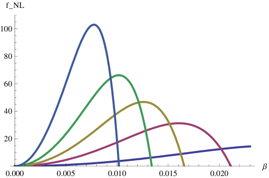
Figure 2: Non-Gaussian parameter $f_{NL}^{\rm local}$ as a function of $\beta$ for several different values of $m^{2}$. The coupling constant parameters are set to $\lambda/g^{4}=1$. The spectral index is set to $n_{S}=0.96$. The curves are, from the one with the highest peak to that with the lowest peak, for $m^{2}=1/20$, $1/23$, $1/25$, $1/27$, and $1/30$.

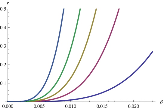
Figure 3: Tensor-to-scalar ratio $r$ as a functions of $\beta$ for several different values of $m^{2}$. The other parameters are the same as in Fig. 2. The curves are, from the left to the right, for $m^{2}=1/20$, $1/23$, $1/25$, $1/27$, and $1/30$.

IV.2 Large mass ratio

Here, we consider the case of large mass ratio. Let us tentatively assume that $m_{1}^{2}\gg m_{2}^{2}$. Then an inspection of Eq. (33) for $f_{NL}^{\rm local}$ suggests that a large $f_{NL}^{\rm local}$ is possible if $W\ll 1$. Hence, let we set $W=0$ for simplicity and investigate this case in detail. We note that the only assumption we adopt is the condition $W=0$; we do not assume a large mass ratio in the following analysis. Namely, the formulas derived below are valid for any mass ratio unless otherwise stated.

The condition $W=0$ implies the following relation between the model parameters:

$$\frac{g_{2}}{g_{1}}\tan\alpha\tan\gamma=\tan\alpha\tan\beta\tan\gamma=1\,.$$ (54)

If $\tan\beta=1$, this means that the inflaton trajectory arrives at the ellipse along the $\phi_{2}$ axis. In this case, Eqs. (24), (25), (26), and (33) respectively reduce to,

$${\cal P}_{S} = \left(\frac{g}{\sigma\,m_{2}^{2}\,e^{m_{2}^{2}N_{k}}}\right)^{2}\frac{1+\cos 2\beta\cos 2\gamma}{2}\left(\frac{H}{2\pi}\right)^{2}_{t_{k}}$$ (55)

$$= \frac{8}{r}\left(\frac{H}{2\pi}\right)^{2}_{t_{k}}\,,$$ (57)

$$n_{S}-1 = 2\,m_{2}^{2}-2\frac{\sigma^{2}}{g^{2}}\frac{m_{1}^{4}e^{2m_{1}^{2}N_{k}}\cot^{2}2\beta\sin^{2}2\gamma+m_{2}^{4}e^{2m_{2}^{2}N_{k}}}{1+\cos 2\beta\cos 2\gamma}$$ (59)

$$= 2\,m_{2}^{2}-\frac{r}{8}\left(\frac{m_{1}^{4}}{m_{2}^{4}}e^{2(m_{1}^{2}-m_{2}^{2})N_{k}}\cot^{2}2\beta\sin^{2}2\gamma+1\right)\,,$$ (61)

$$r = 8\left(\frac{\sigma\,m_{2}^{2}\,e^{m_{2}^{2}N_{k}}}{g}\right)^{2}\frac{2}{1+\cos 2\beta\cos 2\gamma}\,,$$ (63)

$$f_{NL}^{\rm local} = \frac{5}{6}\left\{\frac{m_{1}^{4}}{m_{2}^{2}}\left(\frac{\cos 2\beta\sin 2\gamma}{1+\cos 2\beta\cos 2\gamma}\right)^{2}-m_{2}^{2}\right\}$$ (65)

$$= \frac{5\,m_{2}^{2}}{6}\left\{\frac{m_{1}^{4}}{m_{2}^{4}}\left(\frac{\cos 2\beta\sin 2\gamma}{1+\cos 2\beta\cos 2\gamma}\right)^{2}-1\right\}\,.$$ (67)

We note that the equal-mass limit discussed in the previous subsection can be obtained by setting $m_{1}^{2}=m_{2}^{2}=m^{2}$ in the above equations, because the condition $W=0$ becomes irrelevant in the equal mass limit.

Eq. (67) implies that we may have large non-Gaussianity if $m_{1}^{2}\gg m_{2}^{2}$ and/or $\cos 2\beta\sin 2\gamma/(1+\cos 2\beta\cos 2\gamma)\gg 1$. We also note that in both cases the value of $f_{NL}^{\rm local}$ will be positive. This result is the same as the equal mass case and similar to the case of the linear exponent potential model discussed in Sasaki:2008uc . We suspect that this positivity property may be generically true for all models that are capable of producing large local non-Gaussianity.

First, let us assume that $\cos 2\beta\sin 2\gamma/(1+\cos 2\beta\cos 2\gamma)$ is of the order of unity. Recall that we have $m_{1}^{2}\ll 1$ and $m_{2}^{2}\ll 1$ from the slow-roll condition. Then in order to obtain a large $f_{NL}^{\rm local}$, say $f_{NL}^{\rm local}\sim 50$, we need to have an extremely large mass ratio, $m_{1}^{2}/m_{2}^{2}\sim 50\,m_{1}^{-2}\gg 1$. Then, Eq. (61) implies that $r$ must be extremely small, since we must have $n_{S}-1\ll 1$. Therefore, large non-Gaussianity is possible only in models of very low energy inflation.

In order to look for the possibility of both large $r$ and large $f_{NL}^{\rm local}$, we consider the case of $\cos 2\beta\sin 2\gamma/(1+\cos 2\beta\cos 2\gamma)\gg 1$. As discussed in the previous subsection, this is realized either for $(\beta,\gamma)\to(0,\pi/2)$ or $(\beta,\gamma)\to(\pi/2,0)$. Again, since both limits are equivalent, we focus on the limit $(\beta,\gamma)\to(0,\pi/2)$. In this limit, setting $\pi/2-\gamma=\delta$ again, we have

$${\cal P}_{S} = \frac{8}{r}\left(\frac{H}{2\pi}\right)^{2}_{t_{k}}\sim\left(\frac{g}{\sigma\,m_{2}^{2}\,e^{m_{2}^{2}N_{k}}}\right)^{2}\frac{1}{\beta^{2}+\gamma^{2}}\left(\frac{H}{2\pi}\right)^{2}_{t_{k}}\,,$$ (68)

$$n_{S}-1 \sim 2\,m_{2}^{2}-\frac{r}{8}\left(\frac{m_{1}^{4}}{m_{2}^{4}}e^{2(m_{1}^{2}-m_{2}^{2})N_{k}}\frac{\delta^{2}}{\beta^{2}}+1\right)\,,$$ (70)

$$r \sim 8\left(\frac{\sigma\,m_{2}^{2}\,e^{m_{2}^{2}N_{k}}}{g}\right)^{2}\frac{1}{\beta^{2}+\delta^{2}}\,,$$ (72)

$$f_{NL}^{\rm local} \sim \frac{5}{6}m_{2}^{2}\,\frac{m_{1}^{4}}{m_{2}^{4}}\left(\frac{\delta}{\beta^{2}+\delta^{2}}\right)^{2}\,.$$ (74)

Now, if we have $\beta\ll\delta\ll 1$, we can obtain large $f_{NL}^{\rm local}$. However, again, Eq. (70) for $n_{S}-1$ implies $r$ must be extremely small if $m_{1}^{2}\gg m_{2}^{2}$. In other words, having a large mass ratio does not help in enlarging the parameter region in which both $r$ and $f_{NL}^{\rm local}$ are large.

V conclusion

We analytically investigated the curvature perturbation and its non-Gaussianity in a model of multi-field hybrid inflation, dubbed multi-brid inflation. The model we considered is a two-field hybrid inflation (two-brid inflation) model with the potential mimicking conventional quadratic potentials. The new ingredient of the model is the generalization of the condition for the end of inflation. We considered a very general coupling of the two inflaton fields to a water-fall field.

Then, using the $\delta N$ formula, we derived an analytical expression for the curvature perturbation. Based on this expression, we obtained the curvature perturbation spectrum ${\cal P}_{S}$, the spectral index $n_{S}$, the tensor-to-scalar ratio $r$, and the non-Gaussian parameter $f_{NL}^{\rm local}$. We found that a large positive $f_{NL}^{\rm local}$ is possible in this model. Then, at least for a certain limited range of the parameters, we explicitly showed that it is possible to have large non-Gaussianity while keeping the values of the other quantities consistent with those of the observation. In particular, we showed that when the two inflaton masses are equal, the parameters can be tuned so that they lead to a fairly large tensor-to-scalar ratio, $r\sim 0.1$, as well as a large non-Gaussian parameter, $f_{NL}^{\rm local}\sim 50$. These values will be at a detectable level in the very near future. On the other hand, interestingly, we found that having a large mass ratio in the present model does not help in producing both $r$ and $f_{NL}^{\rm local}$ large enough to be detected. This is in contrast to the model studied in Sasaki:2008uc .

The standard lore has been that $f_{NL}^{\rm local}$ is too small for models with large $r$ or vice versa. We have shown, in this paper, not be the case, particularly in this model of spontaneously symmetry breaking at the end of inflation. This may be the most important conclusion of this work. At the moment, we have no clear physical explanation for this result. We hope we will be able to answer this question in the near future.

Appendix A $\bm{\delta N}$ to Second Order

Here we evaluate $\delta N$ to the second order in the perturbation. We assume the field fluctuations $\delta\phi_{1}$ and $\delta\phi_{2}$ are of linear order.

First, we express the perturbation in the orbital parameter $\gamma$ in terms of $\delta\phi_{1}$ and $\delta\phi_{2}$. Setting $\delta\gamma=\delta_{1}\gamma+\delta_{2}\gamma$, where $\delta_{1}\gamma$ and $\delta_{2}\gamma$ are of linear and second orders, respectively, we take the perturbation of Eq. (17) to the second order. We obtain

$$\left(\frac{1}{m_{1}^{2}}\frac{\delta\phi_{1}}{\phi_{1}}-\frac{1}{2m_{1}^{2}}\frac{\delta\phi_{1}^{2}}{\phi_{1}^{2}}\right)-\left(\frac{1}{m_{2}^{2}}\frac{\delta\phi_{2}}{\phi_{2}}-\frac{1}{2m_{2}^{2}}\frac{\delta\phi_{2}^{2}}{\phi_{2}^{2}}\right)$$

$$\quad=\left(\frac{1}{m_{1}^{2}}\frac{\partial}{\partial\gamma}\ln\phi_{1,f}-\frac{1}{m_{2}^{2}}\frac{\partial}{\partial\gamma}\ln\phi_{2,f}\right)(\delta_{1}\gamma+\delta_{2}\gamma)+\frac{1}{2}\left(\frac{1}{m_{1}^{2}}\frac{\partial^{2}}{\partial\gamma^{2}}\ln\phi_{1,f}-\frac{1}{m_{2}^{2}}\frac{\partial^{2}}{\partial\gamma^{2}}\ln\phi_{2,f}\right)(\delta_{1}\gamma)^{2}.$$ (75)

The linear part of the above equation determines $\delta_{1}\gamma$. We find

$$\delta_{1}\gamma=\frac{\displaystyle\frac{1}{m_{1}^{2}}\frac{\delta\phi_{1}}{\phi_{1}}-\frac{1}{m_{2}^{2}}\frac{\delta\phi_{2}}{\phi_{2}}}{\displaystyle\frac{1}{m_{1}^{2}}\frac{\partial}{\partial\gamma}\ln\phi_{1,f}-\frac{1}{m_{2}^{2}}\frac{\partial}{\partial\gamma}\ln\phi_{2,f}}=\frac{\displaystyle\frac{m_{2}^{2}}{\phi_{1}}\delta\phi_{1}-\frac{m_{1}^{2}}{\phi_{2}}\delta\phi_{2}}{\displaystyle-m_{2}^{2}\frac{Y}{X}+m_{1}^{2}\frac{W}{Z}}\,.$$ (76)

Here, for notational simplicity, we have introduced $X$, $Y$, $Z$ and $W$, which are defined by

$$X = \frac{g_{1}g_{2}}{g\,\sigma}\,\phi_{1,f}=\frac{1}{g}(g_{2}\cos\alpha\cos\gamma-g_{1}\sin\alpha\sin\gamma)\,,$$ (77)

$$Y = -\frac{g_{1}g_{2}}{g\,\sigma}\,\frac{\partial}{\partial\gamma}\phi_{1,f}=\frac{1}{g}(g_{2}\cos\alpha\sin\gamma+g_{1}\sin\alpha\cos\gamma)\,,$$ (79)

$$Z = \frac{g_{1}g_{2}}{g\,\sigma}\,\phi_{2,f}=\frac{1}{g}(g_{2}\sin\alpha\cos\gamma+g_{1}\cos\alpha\sin\gamma)\,,$$ (81)

$$W = -\frac{g_{1}g_{2}}{g\,\sigma}\,\frac{\partial}{\partial\gamma}\phi_{2,f}=\frac{1}{g}(g_{2}\sin\alpha\sin\gamma-g_{1}\cos\alpha\cos\gamma)\,,$$ (83)

where $g=\sqrt{g_{1}^{2}+g_{2}^{2}}$. The factor $1/g$ in front of each of these quantities has been inserted for later convenience.

Then, collecting the second-order terms in Eq. (75), we find

$$\delta_{2}\gamma =\frac{1}{2}\frac{\displaystyle-\frac{\delta\phi_{1}^{2}}{m_{1}^{2}\phi_{1}^{2}}+\frac{\delta\phi_{2}^{2}}{m_{2}^{2}\phi_{2}^{2}}-\left(\frac{1}{m_{1}^{2}}\frac{\partial^{2}}{\partial\gamma^{2}}\ln\phi_{1,f}-\frac{1}{m_{2}^{2}}\frac{\partial^{2}}{\partial\gamma^{2}}\ln\phi_{2,f}\right)(\delta_{1}\gamma)^{2}}{\displaystyle\left(\frac{1}{m_{1}^{2}}\frac{\partial}{\partial\gamma}\ln\phi_{1,f}-\frac{1}{m_{2}^{2}}\frac{\partial}{\partial\gamma}\ln\phi_{2,f}\right)}$$

$$=\frac{1}{2}\frac{\displaystyle\left(\frac{m_{2}}{\phi_{1}}\delta\phi_{1}\right)^{2}-\left(\frac{m_{1}}{\phi_{2}}\delta\phi_{2}\right)^{2}+\left(-m_{2}^{2}\frac{X^{2}+Y^{2}}{X^{2}}+m_{1}^{2}\frac{Z^{2}+W^{2}}{Z^{2}}\right)(\delta_{1}\gamma)^{2}}{\displaystyle m_{2}^{2}\frac{Y}{X}-m_{1}^{2}\frac{W}{Z}}\,,$$ (84)

where we note that

$$X^{2}+Y^{2}=\frac{g_{2}^{2}}{g^{2}}\cos^{2}\alpha+\frac{g_{1}^{2}}{g^{2}}\sin^{2}\alpha\,,\quad Z^{2}+W^{2}=\frac{g_{2}^{2}}{g^{2}}\sin^{2}\alpha+\frac{g_{1}^{2}}{g^{2}}\cos^{2}\alpha\,,$$ (85)

Now, we compute $\delta N$. Although it is straightforward to expand Eq. (11) to the second order in the field fluctuations, the calculation is much simpler if we take the perturbation of either of the solutions $\phi_{1}$ or $\phi_{2}$ of the slow roll equations of motion (6). For example, the solution for $\phi_{1}$ is expressed as

$$\phi_{1}=\phi_{1,f}e^{m_{1}^{2}N}\quad\leftrightarrow\quad N=\frac{1}{m_{1}^{2}}\left(\ln\phi_{1}-\ln\phi_{1,f}\right)\,.$$ (86)

The perturbation of the second equation gives

$$\delta N=\frac{1}{m_{1}^{2}}\left[\frac{\delta\phi_{1}}{\phi_{1}}-\frac{\partial}{\partial\gamma}\ln\phi_{1,f}\,\delta_{1}\gamma-\frac{1}{2}\left(\frac{\delta\phi_{1}}{\phi_{1}}\right)^{2}-\frac{1}{2}\frac{\partial^{2}}{\partial\gamma^{2}}\ln\phi_{1,f}\,(\delta_{1}\gamma)^{2}-\frac{\partial}{\partial\gamma}\ln\phi_{1,f}\,\delta_{2}\gamma\right]\,.$$ (87)

Inserting Eqs. (76) and (84) into Eq. (87), we obtain

$$\delta N=\frac{\displaystyle-\frac{W}{Z}\frac{\delta\phi_{1}}{\phi_{1}}+\frac{Y}{X}\frac{\delta\phi_{2}}{\phi_{2}}}{\displaystyle m_{2}^{2}\frac{Y}{X}-m_{1}^{2}\frac{W}{Z}}+\frac{1}{2}\frac{\displaystyle\frac{W}{Z}\left(\frac{\delta\phi_{1}}{\phi_{1}}\right)^{2}-\frac{Y}{X}\left(\frac{\delta\phi_{2}}{\phi_{2}}\right)^{2}}{\displaystyle m_{2}^{2}\frac{Y}{X}-m_{1}^{2}\frac{W}{Z}}-\frac{1}{2}\frac{\displaystyle\left(1-\frac{YW}{XZ}\right)\left(\frac{W}{Z}-\frac{Y}{X}\right)\left(\frac{m_{2}^{2}}{\phi_{1}}\delta\phi_{1}-\frac{m_{1}^{2}}{\phi_{2}}\delta\phi_{2}\right)^{2}}{\displaystyle\left(m_{2}^{2}\frac{Y}{X}-m_{1}^{2}\frac{W}{Z}\right)^{3}}\,.$$ (88)

Finally, we mention that we can divide $\delta N$ into two contributions: one from during inflation up to a surface of constant potential energy, $\delta N_{*}$, and the contribution from the end of inflation, $\delta N_{e}$. In the case of the exponential potential model considered in Sasaki:2008uc , there was no non-Gaussianity in $\delta N_{*}$ to the lowest order in the slow-roll parameters. In contrast, there exists non-Gaussianity in $\delta N_{*}$ in the present model. Nevertheless, it can be easily shown that it is of the order of the slow-roll parameters, and hence is negligibly small.

Appendix B Linear Exponential Potential Model

In this appendix, we consider the case of a linear exponential potential,

$$V=V_{0}\exp(m_{1}\phi_{1}+m_{2}\phi_{2})\,,$$ (89)

with the condition for the end of inflation given by

$$\sigma^{2}=g_{1}^{2}(\phi_{1}\cos\alpha+\phi_{2}\sin\alpha)^{2}+g_{2}^{2}(-\phi_{1}\sin\alpha+\phi_{2}\cos\alpha)^{2}\,.$$ (90)

This model was discussed in Sasaki:2008uc . However, it was assumed that $\alpha=0$. Here, for the sake of completeness, we consider the general condition adopted in the main text.

As in §2, we parametrize the scalar field at the end of inflation as

$$\frac{\sigma}{g_{1}}\cos\gamma=\phi_{1,f}\cos\alpha+\phi_{2,f}\sin\alpha\,,\quad\frac{\sigma}{g_{2}}\sin\gamma=-\phi_{1,f}\sin\alpha+\phi_{2,f}\cos\alpha\,,$$ (91)

or, conversely,

$$\phi_{1,f}=\frac{\sigma}{g_{1}g_{2}}(g_{2}\cos\alpha\cos\gamma-g_{1}\sin\alpha\sin\gamma)\,,\quad\phi_{2,f}=\frac{\sigma}{g_{1}g_{2}}(g_{2}\sin\alpha\cos\gamma+g_{1}\cos\alpha\sin\gamma)\,.$$ (92)

Also, as before, we introduce $g=\sqrt{g_{1}^{2}+g_{2}^{2}}$, and $X$, $Y$, $Z$ and $W$ as

$$X = \frac{g_{1}g_{2}}{g\,\sigma}\,\phi_{1,f}=\frac{1}{g}(g_{2}\cos\alpha\cos\gamma-g_{1}\sin\alpha\sin\gamma)\,,$$ (93)

$$Y = -\frac{g_{1}g_{2}}{g\,\sigma}\,\frac{\partial}{\partial\gamma}\phi_{1,f}=\frac{1}{g}(g_{2}\cos\alpha\sin\gamma+g_{1}\sin\alpha\cos\gamma)\,,$$ (95)

$$Z = \frac{g_{1}g_{2}}{g\,\sigma}\,\phi_{2,f}=\frac{1}{g}(g_{2}\sin\alpha\cos\gamma+g_{1}\cos\alpha\sin\gamma)\,,$$ (97)

$$W = -\frac{g_{1}g_{2}}{g\,\sigma}\,\frac{\partial}{\partial\gamma}\phi_{2,f}=\frac{1}{g}(g_{2}\sin\alpha\sin\gamma-g_{1}\cos\alpha\cos\gamma)\,.$$ (99)

Let us calculate the curvature perturbation for this model. To begin with, we evaluate the perturbation in $\gamma$ to the second order to obtain

$$\delta_{1}\gamma=-\frac{g_{1}g_{2}}{g\,\sigma}\frac{m_{2}\delta\phi_{1}-m_{1}\delta\phi_{2}}{m_{2}Y-m_{1}W}\,,\quad\delta_{2}\gamma=-\frac{(\delta_{1}\gamma)^{2}}{2}\frac{m_{2}X-m_{1}Z}{m_{2}Y-m_{1}W}\,.$$ (100)

On the basis of these equations, $\delta N$ is evaluated to the second order as

$$\delta N=\frac{-W\delta\phi_{1}+Y\delta\phi_{2}}{m_{2}Y-m_{1}W}+\frac{(g_{1}g_{2})^{2}}{2g^{3}\sigma}\frac{(m_{2}\delta\phi_{1}-m_{1}\delta\phi_{2})^{2}}{(m_{2}Y-m_{1}W)^{3}}\,.$$ (101)

Now we can evaluate the quantities of interest. As before, for convenience, we introduce angle $\beta$ as

$$g_{1}=g\cos\beta\,,\quad g_{2}=g\sin\beta\,.$$ (102)

Then the curvature perturbation spectrum is

$${\cal P}_{S}=\frac{Y^{2}+W^{2}}{(m_{2}Y-m_{1}W)^{2}}\left(\frac{H}{2\pi}\right)^{2}_{t_{k}}\,.$$ (103)

The spectral index is

$$n_{S}=1-(m_{1}^{2}+m_{2}^{2})\,.$$ (104)

The tensor-to-scalar ratio is

$$r=8\frac{(m_{2}Y-m_{1}W)^{2}}{Y^{2}+W^{2}}\,.$$ (105)

Finally, the non-Gaussianity is

$$f_{NL}^{\rm local}=\frac{5g}{6\sigma}\frac{\cos^{2}\beta\sin^{2}\beta\,(m_{1}Y+m_{2}W)^{2}}{(Y^{2}+W^{2})^{2}(m_{2}Y-m_{1}W)}\,,$$ (106)

where we note that

$$Y^{2}+W^{2}=\cos^{2}\beta\cos^{2}\gamma+\sin^{2}\beta\sin^{2}\gamma\,.$$ (107)

Here, it is worthwhile to mention that the spectral index depends only on $m_{1}$ and $m_{2}$.

To enable a direct comparison with the model discussed in the main text, let us consider the case of $W=0$ for the present model as well. In this case, we have

$${\cal P}_{S} = \frac{1}{m_{2}^{2}}\left(\frac{H}{2\pi}\right)^{2}_{t_{k}}\,,$$ (108)

$$r = 8\,m_{2}^{2}\,,$$ (110)

$$f_{NL}^{\rm local} = \frac{5g}{6\sigma}\frac{\cos^{2}\beta\sin^{2}\beta}{(\cos^{2}\beta\cos^{2}\gamma+\sin^{2}\beta\sin^{2}\gamma)^{3/2}}\frac{m_{1}^{2}}{m_{2}}\,.$$ (112)

We see that a large mass ratio, $m_{1}\gg m_{2}$, is necessary in order to realize a large $f_{NL}^{\rm local}$. However, because $r$ in the present case is determined only by the smaller mass, $r=8\,m_{2}^{2}$, it is difficult to realize both large $r$ and large $f_{NL}^{\rm local}$ . This is in contrast to the case we discussed in the main text, for which it was possible to make both values large enough to be detectable in the very near future.

References

- (1) D. S. Salopek and J. R. Bond, Phys. Rev. D 42 (1990), 3936 .
- (2) E. Komatsu and D. N. Spergel, Phys. Rev. D 63 (2001), 063002; astro-ph/0005036.
- (3) D. Babich and M. Zaldarriaga, Phys. Rev. D 70 (2004), 083005; astro-ph/0408455.
-
(4)
F. Bernardeau and J. P. Uzan,
Phys. Rev. D 66 (2002), 103506;
hep-ph/0207295.
N. Bartolo, S. Matarrese and A. Riotto, Phys. Rev. D 69 (2004), 043503; hep-ph/0309033.
C. Gordon and K. A. Malik, Phys. Rev. D 69 (2004), 063508; astro-ph/0311102.
K. Enqvist and S. Nurmi, J. Cosmol. Astropart 0510 (2005), 013; astro-ph/0508573.
D. H. Lyth, Nucl. Phys. Proc. Suppl. 148 (2005), 25.
K. A. Malik and D. H. Lyth, J. Cosmol. Astropart 0609 (2006), 008; astro-ph/0604387.
M. Sasaki, J. Valiviita and D. Wands, Phys. Rev. D 74 (2006), 103003; astro-ph/0607627.
J. Valiviita, M. Sasaki and D. Wands, astro-ph/0610001.
S. Yokoyama, T. Suyama and T. Tanaka, J. Cosmol. Astropart 0707 (2007), 013; arXiv:0705.3178.
S. Yokoyama, T. Suyama and T. Tanaka, arXiv:0711.2920.
K. Ichikawa, T. Suyama, T. Takahashi and M. Yamaguchi, arXiv:0802.4138.
T. Suyama and F. Takahashi, arXiv:0804.0425.
T. Matsuda, arXiv:0804.3268.
F. Bernardeau and T. Brunier, Phys. Rev. D 76 (2007), 043526; arXiv:0705.2501.
D. A. Easson, R. Gregory, D. F. Mota, G. Tasinato and I. Zavala, J. Cosmol. Astropart 0802 (2008), 010; arXiv:0709.2666. -
(5)
M. Zaldarriaga,
Phys. Rev. D 69 (2004), 043508;
astro-ph/0306006.
G. N. Felder and L. Kofman, hep-ph/0606256.
T. Suyama and M. Yamaguchi, Phys. Rev. D 77 (2008), 023505; arXiv:0709.2545.
F. Bernardeau, L. Kofman and J. P. Uzan, Phys. Rev. D 70 (2004), 083004; astro-ph/0403315. - (6) F. Bernardeau and J. P. Uzan, Phys. Rev. D 67 (2003), 121301; astro-ph/0209330.
- (7) G. Dvali, A. Gruzinov and M. Zaldarriaga, Phys. Rev. D 69 (2004), 023505; astro-ph/0303591.
- (8) L. Kofman, astro-ph/0303614.
- (9) D. H. Lyth, J. Cosmol. Astropart 0511 (2005), 006; astro-ph/0510443.
-
(10)
L. Alabidi and D. Lyth,
J. Cosmol. Astropart 0608 (2006), 006;
astro-ph/0604569.
L. Alabidi, J. Cosmol. Astropart 0610 (2006), 015; astro-ph/0604611. -
(11)
N. Barnaby and J. M. Cline,
Phys. Rev. D 75 (2007), 086004;
astro-ph/0611750.
N. Barnaby and J. M. Cline, J. Cosmol. Astropart 0707 (2007), 017; arXiv:0704.3426.
N. Barnaby and J. M. Cline, J. Cosmol. Astropart 0806 (2008), 030; arXiv:0802.3218. - (12) A. Chambers and A. Rajantie, Phys. Rev. Lett. 100 (2008), 041302; arXiv:0710.4133.
- (13) E. Silverstein and D. Tong, Phys. Rev. D 70 (2004), 103505; hep-th/0310221.
-
(14)
M. Alishahiha, E. Silverstein and D. Tong,
Phys. Rev. D 70 (2004), 123505;
hep-th/0404084.
D. Seery and J. E. Lidsey, J. Cosmol. Astropart 0506 (2005), 003; astro-ph/0503692.
X. Chen, M. X. Huang, S. Kachru and G. Shiu, J. Cosmol. Astropart 0701 (2007), 002; hep-th/0605045.
M. X. Huang, G. Shiu and B. Underwood, Phys. Rev. D 77 (2008), 023511; arXiv:0709.3299.
D. Langlois, S. Renaux-Petel, D. A. Steer and T. Tanaka, arXiv:0804.3139. arXiv:0806.0336.
F. Arroja, S. Mizuno and K. Koyama, arXiv:0806.0619. - (15) M. Sasaki, Prog. Theor. Phys. 120 (2008), 159; arXiv:0805.0974 .
- (16) M. Sasaki and E. D. Stewart, Prog. Theor. Phys. 95 (1996), 71; astro-ph/9507001.
- (17) M. Sasaki and T. Tanaka, Prog. Theor. Phys. 99 (1998), 763; gr-qc/9801017.
- (18) D. Wands, K. A. Malik, D. H. Lyth and A. R. Liddle, Phys. Rev. D 62 (2000), 043527; astro-ph/0003278.
- (19) D. H. Lyth, K. A. Malik and M. Sasaki, J. Cosmol. Astropart 0505 (2005), 004; astro-ph/0411220.
- (20) D. H. Lyth and Y. Rodriguez, Phys. Rev. Lett. 95 (2005), 121302; astro-ph/0504045.
- (21) H. R. S. Cogollo, Y. Rodriguez and C. A. Valenzuela-Toledo, J. Cosmol. Astropart 0808 (2008), 029; arXiv:0806.1546.
- (22) M. Sasaki, Class. Quantum. Grav. 24 (2007), 2433; astro-ph/0702182.
- (23) A. A. Starobinsky, JETP Lett. 42 (1985) 152 [Pisma Zh. Eksp. Teor. Fiz. 42 (1985) 124].
- (24) A. R. Liddle, D. Parkinson, S. M. Leach and P. Mukherjee, Phys. Rev. D 74 (2006), 083512; astro-ph/0607275.
- (25) J. Dunkley et al. (WMAP Collaboration), arXiv:0803.0586.
- (26) E. Komatsu et al. (WMAP Collaboration), arXiv:0803.0547.