The variable super-orbital modulation of Cygnus X-1

Abstract

We study the super-orbital modulation present in the Cygnus X-1 X-ray data, usually attributed to the precession of the accretion disk and relativistic jets. We find a new, strong, 326$\pm$2 d period modulation starting in 2005, in Swift/BAT and RXTE/ASM light curves (LCs). We also investigate Vela 5B/ASM and Ariel V/ASM archival data and confirm the previously reported $\sim$290 d periodic modulation, and therefore confirming that the super-orbital period is not constant. Finally, we study RXTE/ASM LC before 2005 and find that the previously reported $\sim$150 d period is most likely an artifact due to the use of a Fourier-power based analysis under the assumption that the modulation has a constant period along the whole data sample. Instead, we find strong indications of several discrete changes of the precession period, happening in coincidence with soft and failed state-transition episodes. We also find a hint of correlation between the period and the amplitude of the modulation. The detection of gamma-rays above 100 GeV with MAGIC in September 2006 happened in coincidence with a maximum of the super-orbital modulation. The next maximum will happen between 2 and 14 of July 2008, when the observational conditions of Cygnus X-1 with ground-based Cherenkov telescopes, such as MAGIC and VERITAS, are optimal.

1. Introduction

Cygnus X-1(Bowyer et al., 1965) is the best established candidate for a stellar mass black-hole (BH). It is composed of a $21\pm 8$ M_⊙ BH turning around an O9.7 Iab companion of $40\pm 10$ M_⊙ (Ziółkowski, 2005) in a circular orbit of 5.6 days (Brocksopp et al., 1999a). High resolution radio imaging has unveiled the presence of a highly colimated, relativistic (Stirling et al., 2001), radiatively inefficient (Gallo et al., 2005) jet. The X-ray source displays soft and hard states and relatively frequent failed transitions between them. There are strong evidences of a high energy non-thermal component extending up to soft gamma-rays (McConnell et al., 2002; Cadolle Bel et al., 2006). The steady emission of gamma-rays above 100 GeV is strongly constrained by the observations with MAGIC which has obtained, however, a very strong evidence of an intense, fast flaring episode at these energies (Albert et al., 2007).

A $\sim$5.6 d period modulation, attributed to the orbital motion of the compact object around the companion, has been observed at various wavelengths by numerous authors (e.g., Pooley et al., 1999; Brocksopp et al., 1999a, b; LaSala et al., 1998; Lachowicz et al., 2006). On the other hand, a super-orbital $\sim$290 d period was claimed by Priedhorsky, Terrel & Holt (1983) on the soft X-ray data recorded by Vela 5B/ASM (1969-1979) and Ariel V/ASM (1974-1980). Later, a $\sim$150 d periodic variability has been reported by various authors (Pooley et al., 1999; Brocksopp et al., 1999b; Ozdemir & Demircan, 2001; Benlloch et al., 2001, 2004; Lachowicz et al., 2006) using different data samples ranging between April 1991 and November 2003. It must be noted, however, that other significant modulations with periods $\sim$200 d and $\sim$420 d have been also found (e.g. Benlloch et al., 2001, 2004; Lachowicz et al., 2006).

In this letter, we search the latest Cygnus X-1 X-ray data for periodic modulations. We also perform a critical revision of the previous results obtained from archival X-ray data. Finally, we put our results in the context of a multiwavelength description of the source.

2. Data samples

Table 1Cygnus X-1 analyzed data

Instrument/	Energy	Operation	Start	End	Time	Number of	$\nu_{1}$	$\nu_{m/2}$
subsample	[keV]	time	[MJD]	[MJD]	span [d]	points (m)	[d-1]	[d-1]
Vela 5B/ASM	3-12	May 1969–Jun 1979	40368	44042	3675	1097	2.7$\times 10^{-4}$	0.15
Ariel V/ASM	3-6	Feb 1976–Feb 1980	42830	44292	1464	740	6.8$\times 10^{-4}$	0.25
RXTE/ASM 1	2-10	Sep 1996–Sep 1999	50328	51444	1117	913	9.0$\times 10^{-4}$	0.41
RXTE/ASM 2	2-10	Jun 2005–May 2008	53529	54592	1064	909	9.4$\times 10^{-4}$	0.43
Swift/BAT	15-150	Jun 2005–May 2008	53529	54598	1070	829	9.3$\times 10^{-4}$	0.39

The data samples analyzed in this work are summarized in Table 1. They are available through the High Energy Astrophysics Archive Research Center (HEASARC). We use data from four different instruments, namely: Vela 5B/ASM, Ariel V/ASM  RXTE/ASM and Swift/BAT. All data are averaged into one-day bins, except when explicitely stated. No periodic behavior is found in the X-ray data during the soft state (Wen et al., 1999; Lachowicz et al., 2006) and therefore we analyze data corresponding to the hard state data only. The interval MJD 42338–42829 is dominated by soft flare events (Liang & Nolan, 1984) and hence excluded from Vela 5B/ASM and Ariel V/ASM analyses. The soft state periods during the operation of RXTE/ASM are identified as those for which the ratio of count rates in the bands C (5.0-12.1 keV) and A (1.3–3.0 keV) is lower than 1.2 and the total count rate exceeds the mean value by more than 4 standard deviations. The mean and standard deviations are computed from the interval MJD 50660–50990 (Lachowicz et al., 2006). This excludes from the analysis the following periods (MJD): 50087–50327, 50645–50652, 51002–51026, 51369–51397, 51445–51625, 51776–51952, 52093–52584, 52762–52878, 52982–53092, 53198–53528, 53780–53872. After this, two long intervals dominated by hard state (samples A and B in Table 1) are defined and studied separately. Based on the results for RXTE/ASM, the intervals 53414–53528 and 53780–53872 are also removed from the analysis of Swift/BAT LC.

3. Analysis

We search the different data samples for periodic signals using the Lomb-Scargle (L-S) test of uniformity (Lomb, 1976; Scargle, 1982). The chance probability is the probability of obtaining a certain L-S test value ($z_{0}$) or larger out of a purely Gaussian noise sample, and is given by ${\cal P}_{\textrm{pre}}(z>z_{0})=e^{-z_{0}}$. When several frequencies are inspected, the post-trial probability, i.e. the probability to get a L-S test value $z_{0}$ or higher for at least one of the scanned frequencies, is given then by ${\cal P}_{\textrm{post}}(z>z_{0})=1-[1-{\cal P}_{\textrm{pre}}(z>z_{0})]^{n}$ where $n$ is the number of independent scanned frequencies.

Given $m$ data points, there is a discrete finite set of $m/2$ independent frequencies. For the case of evenly spaced data there is a natural set of frequencies: $\nu_{k}=\frac{k}{T}$ ($k=1,\dots,m/2$) where $T$ is the time spanned by the data set. The values of the Fourier transform powers for the natural frequencies are independent of one another. The data set does not contain enough information to search for periodicities below $\nu_{1}=1/T$ or above $\nu_{m/2}=m/2T$. The time span, number of data points and the maximum and minimum accessible frequencies for the different studied data samples are shown in Table 1.

For each investigated data sample we produce the periodogram, where $-\log_{10}({\cal P}_{\textrm{post}})$ is represented as a function of the frequency. A prominent periodic component in the data is visible as a peak in the periodogram at the relevant frequency ($\nu_{\textrm{peak}}$). We consider as significant those peaks for which the post-trial probability is lower than $10^{-6.5}$, equivalent to a deviation of 5$\sigma$ from the Gaussian noise case. We scan all natural frequencies, with an oversampling factor of 5. This means that we scan $5m/2$ evenly spaced frequencies, from $\nu_{1}$ to $\nu_{m/2}$. The oversampling does not increase the number of trials in the post-trial chance probability, since the number of independent frequencies remains constant, but increases the precision of $\nu_{\textrm{peak}}$. To estimate the error ($\Delta$$\nu_{\textrm{peak}}$), we use the standard deviation of $\nu_{\textrm{peak}}$ over 100 random data samples obtained by bootstrap (Davison & Hinkley, 2006) of the original LC. Then, we fold the LC into a phaseogram using the period $1/$$\nu_{\textrm{peak}}$. The phaseogram is produced using 50 bins, to ensure a smooth description of the waveform. The time of the phase 0 ($T_{0}$) is determined from a fit to the LC using a Cosine function, where the value of the frequency is fixed to $\nu_{\textrm{peak}}$. In this way, $T_{0}$ corresponds to the maximum of the fitting Cosine function (although not necessarily to the maximum of the waveform). The modulation amplitude ($A$) is defined as the ratio between the amplitude and the mean value of the Cosine function obtained from the fit. Finally, we remove the periodic component of frequency $\nu_{\textrm{peak}}$ from the LC (a process called prewhitening). This is done by subtracting the deviations of the phaseogram from its mean value throughout the LC.

We subsequently search for the next most prominent peak in the prewhitened LC, and follow the whole process described above in an iterative fashion. This process is stopped when the obtained $\nu_{\textrm{peak}}$ has a post-trial chance probability larger then $10^{-6.5}$.

4. Results

We first search for periodic signals in Swift/BAT and RXTE/ASM 2 data samples, which correspond to the same epoch, and which are analyzed in this work for the first time. The results are shown in Table 2. The L-S periodograms for both LCs are shown in Figure 1. A very strong, dominant periodic signal with period 326$\pm$2 d is found in both data samples. The LCs are shown in Figure 2. The modulation is clearly seen by eye, which is reflected by the extremely low values of ${\cal P}_{\textrm{post}}$. The previously reported $\sim$150 d modulation is not found in these data. The pre-trial chance probabilities for such a modulation are $10^{-1.3}$ and $10^{-0.1}$ for RXTE/ASM and Swift/BAT data, respectively. Figure 1 shows the $\sim 150$ d modulation as reported by Lachowicz et al. (2006) overlaid with RXTE/ASM 2 LC, confirming that such a modulation does not describe well the data. The phaseograms corresponding to the 326 d period are shown in Figure 3. We see that hard and soft X-ray LCs are strongly correlated, with Pearson’s correlation factor $r=0.97$. A second, also strong, component with period $\sim$1000 d is present in both data samples. This corresponds to a long-term modulation of the X-ray flux with respect to the 326 d oscillation, but cannot be established as periodic since the period is similar to the total time spanned by the observations. An alternative explanation to the $\sim$1000 d period will be given below. Finally, a third component is seen in RXTE/ASM 2 data sample at period $\sim$5.6 d, compatible with the orbital modulation, visible in the periodogram (Figure 1) even before prewhitening. This modulation is not seen in Swift/BAT data, for which ${\cal P}_{\textrm{pre}}\simeq 10^{-2}$. On a similar energy band, Paciesas et al. (1997) claimed a modulation compatible with the orbital period in CGRO/BATSE LC between April 1991 and September 1996, but the method used lacks of a mathematical justification. Brocksopp et al. (1999b) did not find any evidence for the orbital modulation in CGRO/BATSE data between May 1996 and September 1998. Finally, Lachowicz et al. (2006), using the whole BATSE light curve, reported a deviation of $\sim 1\sigma$ from the Gaussian noise case, insufficient to establish the presence of the orbital modulation in the data.

We have searched Vela 5B/ASM and Ariel V/ASM LCs for periodic modulations and found peaks at P=(276$\pm$3) d and P=(288$\pm$3) d, respectively (see Table 2), in agreement with the results obtained by Priedhorsky, Terrel & Holt (1983) and Lachowicz et al. (2006). By comparison with the P=(326$\pm$3) d present in Swift/BATand RXTE/ASM 2 LC, this shows that the period of the super-orbital modulation is variable. The corresponding phaseograms are shown if Figure 3 (two lowermost panels). Even if the relative dispersion of the points is larger due to the lower sensitivity of Ariel V/ASM and Vela 5B/ASM, the waveform is still visible. They follow a very similar shape as those found for Swift/BAT and RXTE/ASM 2, albeit for a different period, as one expects if the underlying physical process is the same. The correlation factor for Swift/BAT and Ariel V/ASM (Vela 5B/ASM) phaseograms is $r=0.73$ ($r=0.57$). However, the modulation amplitudes are significantly lower than for the case of RXTE/ASM. This could have a physical explanation, but it could also happen if the periodic modulation was not present in part of the LCs, which can be certainly not excluded. On the other hand, we do not find evidence for the orbital period in Vela 5B/ASM or Ariel V/ASM LCs. It is worth noting that, given Vela 5B/ASM and Ariel V/ASM sensitivities, we do not expect to detect an orbital modulation with an amplitude of $\sim$5$\%$ as the one we see in RXTE/ASM 2 data. The mean relative variance of the data points in the phaseogram (which is a good estimate of the measurement error) are $46\%$ and $13\%$ for Vela 5B/ASM and Ariel V/ASM  respectively. Both values are well above the $5\%$ modulation which is hence difficult to detect. We have crosschecked this by analyzing Monte Carlo (MC) simulated LCs for Vela 5B/ASM and Ariel V/ASM. We use the same sampling as the measured LCs and simulate a $5\%$ amplitude modulation convolved with $46\%$ and $13\%$ point-to-point random fluctuations, respectively. The analysis of these LCs yields no significant peak.

Table 2Results for periodic signal search

Sample	P${}_{\textrm{peak}}$		$T_{0}$	$A$	${\cal P}_{\textrm{post}}$
	[d]		[MJD]	[$\%$]
Swift/BAT	326$\pm$	2	54027.3	25	$10^{-87}$
	1030$\pm$	50	53707.2	6	$10^{-10}$
RXTE/ASM 2	326$\pm$	2	54032.2	29	$10^{-96}$
	990$\pm$	30	53670.7	13	$10^{-41}$
	5.600$\pm$	0.002	53670.3	5	$10^{-11}$
RXTE/ASM 1a	248$\pm$	9	50377.2	29	$10^{-30}$
RXTE/ASM 1b	123$\pm$	3	50761.1	11	$10^{-10}$
RXTE/ASM 1c	168$\pm$	4	51177.6	18	$10^{-24}$
RXTE/ASM 1	5.602$\pm$	0.002	51117.1	4.1	$10^{-7.1}$
Ariel V/ASM	276$\pm$	3	42865.8	14	$10^{-16}$
Vela 5B/ASM	288$\pm$	3	40187.4	21	$10^{-6.8}$

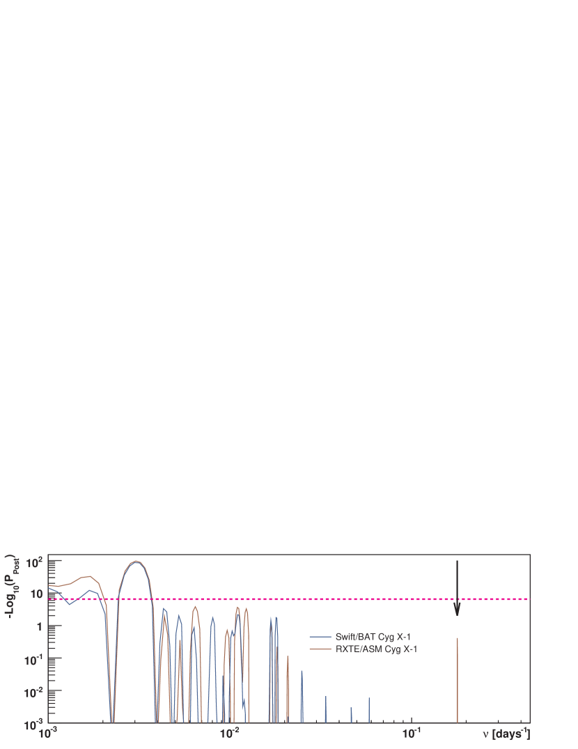
Figure 1.— Periodograms for Swift/BAT and RXTE/ASM 2 Cygnus X-1 samples, showing the post-trial chance probability as a function of the scanned frequency. The horizontal line marks the line corresponding to a post-trial probability of $10^{-6.5}$. The arrow marks the orbital frequency.

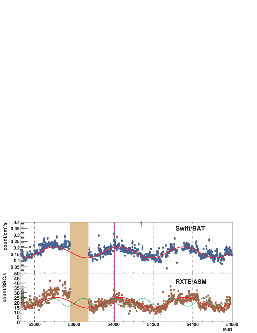
Figure 2.— Swift/BAT  and RXTE/ASM 2 LCs. The shaded area shows an interval of soft state, identified by the criteria exposed in Section 2, and not considered in the analysis. The thick, red curves are the fits by Cosine functions to each subsample (see Section 3). The thin, green curve represents the $\sim 150$ d super-orbital modulation using the ephemeris reported by Lachowicz et al. (2006). The vertical, purple line marks the time of the TeV signal reported by Albert et al. (2007)

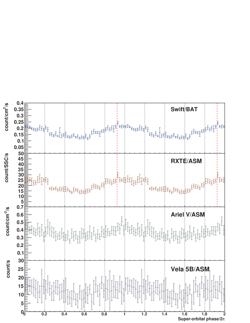
Figure 3.— From top to bottom: Swift/BAT, RXTE/ASM 2, Ariel V/ASM and Vela 5B/ASM phaseograms folded using period P and time 0 values (P [d],$T_{0}\textrm{[MJD]}$)= (326, 54027), (326, 54027), (276, 42866) and (288, 40187), respectively. The values of $T_{0}$ are obtained from the fit of a Cosine function. Data points and error bars correspond, respectively, to the mean count rate and variance measured within each phase bin. The vertical, red, dashed line corresponds to the phase of the TeV signal reported by Albert et al. (2007).

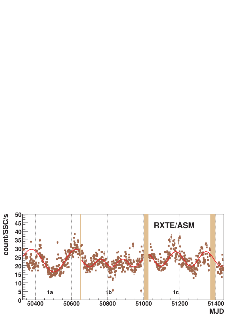
Figure 4.— RXTE/ASM 1 light curve. The vertical shaded lines show the intervals of soft or failed transition states, identified by the criteria exposed in Section 2, which delimit the three subsamples (1a, 1b and 1c) used for further analysis. The red curves are the fits by Cosine functions to each subsample (see Section 3).

Finally, we have searched RXTE/ASM 1 data sample for periodic modulations, and found 5 significant peaks at P = (148$\pm$1), (188$\pm$2), (310$\pm$11), (475$\pm$11) and (5.598$\pm$0.003) d, all with chance probabilities lower than $10^{-10}$. The latter corresponds to the orbital modulation, whereas the other four seem to denote a complex power spectrum. We stress that some of these peaks have been found in previous studies of the RXTE/ASM LC (Benlloch et al., 2001, 2004; Lachowicz et al., 2006). The understanding of the super-orbital modulation can be greatly simplified if we consider that the period can change along the observation time in a discrete way. We have analyzed separately the data between each two consecutive soft or failed transition states, i.e. three samples, namely 1a=[50328–50644], 1b=[50653–51001] and 1c=[51027–51368] (see Figure 4). We obtain a single significant peak in each of them (see Table 2). We prewhiten the leading frequency in each of the subsamples and merge them to look for sub-leading frequencies. The only remaining significant peak corresponds to the orbital modulation (see Table 2). Figure 4 shows RXTE/ASM 1 LC, overlaid with the result of the fits to independent Cosine functions to the three defined subsamples. The general agreement with the data is remarkably good. We have also generated three MC samples corresponding to the samplings of 1a, 1b and 1c subsamples, and pure sinusoidal modulations with the periods found for each of them, convolved with the measured point-to-point fluctuations. Then we have merged the three samples together and analyzed the resulting LC. We obtain significant peaks at P = (147$\pm$1), (190$\pm$2) and (523$\pm$12) d, in surprisingly good agreement with the results of analyzing the real data. We note that this effect could be also responsible of the $\sim$1000 d periodicity of the Swift/BAT and RXTE/ASM 2 data, since they also contain a soft state episode that might have changed the period of the super-orbital modulation prior to MJD=53780.

5. Discussion

We find that Cygnus X-1 displays a super-orbital modulation, with a period that changes, probably in a discrete way and in coincidence with soft or failed state-transition phases, over time scales ranging from a few hundred days to several years. According to our findings, the very much cited $\sim$150 d period is most probably an artifact of applying a (sometimes biased) Fourier-transform based analysis to a data sample where more than one consecutive period modulations are present. Since 2005, Cygnus X-1 shows a very powerful and stable super-orbital modulation with a period of $326\pm 2$ d.

The super-orbital modulation is usually attributed to the precession of the accretion disk (Priedhorsky, Terrel & Holt, 1983) and relativistic jet (Romero, Kaufman Bernadó & Mirabel, 2002), as a result of the tidal forces exerted by the companion star on a tilted disk (Katz, 1973). A mechanism for keeping the disk tilted can be provided by radiation pressure warping (Petterson, 1977; Pringle, 1996; Wijers & Pringle, 1999; Ogilvie & Dubus, 2001). In the case of tidally forced precession, the expected period $P_{\textrm{prec}}$ depends on the outer radius $R_{o}$ and inclination of the disk $\delta$ as $P_{\textrm{prec}}\propto R_{o}^{-3/2}\cos^{-1}\delta$ (Larwood, 1998). Then, the longer the period the larger the precession angle, and hence also a larger modulation amplitude is expected. This is in agreement with our results for RXTE/ASM, where we have found four different super-orbital periods, which follow this tendency (see Table 2 and Figure 4).

A different issue is why the precession of the disk produces a modulation in the X-ray flux. Some authors (e.g., Lachowicz et al., 2006; Ibragimov, Zdziarski & Poutanen, 2007) have considered the possibility that the precession movement changes the optical thickness along the line of sight. They reject this possibility since it seems unlikely due to the fine tuning required to produce the observed modulation amplitude, which in addition should depend on the energy, which is not confirmed by our observations. The multiwavelenth data seem to support a scenario where the emission itself is anisotropic. The precession modulation is detected at similar times with identical periods in radio, soft and hard X-rays during the hard state. A unified picture, where the anisotropy is provided by the jet, has been proposed by Brocksopp et al. (1999b). The soft X-ray emission is produced in the disk via bremsstrahlung of thermal electrons, and are then up-scattered to higher energies via Compton scattering in the hot corona or at the base of the relativistic jet (which precesses with the disk). The acceleration of electrons along magnetic field lines in the jet produces the radio emission by synchrotron emission. During the soft state, the jet and corona dissappear and no modulation is observed. According to our findings, once the source goes back to the hard state, the reconstructed disk and jet have different kinematical properties, and the modulation period changes. It seems that failed transitions produce a similar effect.

MAGIC detected a fast and intense episode of emission of gamma-rays above 100 GeV (Albert et al., 2007) during MJD=54003, albeit at the limit of the telescope’s sensitivity. This happened in coincidence with the soft and hard X-ray maxima (Figures 2 and 3) and an unusually bright outburst detected with INTEGRAL (Malzac et al., 2008). It is interesting to note that, according to the ephemeris shown in Table 2, the next passage for the precession maximum will happen at MJD=54655$\pm$2, i.e. between 6 and 10 of July 2008. The observational conditions of Cygnus X-1 with ground-based Cherenkov telescopes, such as MAGIC and VERITAS, will be optimal during those days.

References

- Albert et al. (2007) Albert, J., et al. 2007, ApJ 665, L51
- Benlloch et al. (2001) Benlloch, S., et al., 2001, ESASP, 459, 236
- Benlloch et al. (2004) Benlloch, S. et al., 2004, AIPC, 714, 61
- Bowyer et al. (1965) Bowyer, S., Byram, E. T., Chubb, T. A., & Friedman, H. 1965, Science, 147, 394
- Brocksopp et al. (1999a) Brocksopp, C., et al. 1999a, MNRAS, 309, 1063
- Brocksopp et al. (1999b) Brocksopp, C., et al., 1999b, A&A 343, 861
- Cadolle Bel et al. (2006) Cadolle Bel, M., et al. 2006, A&A, 446, 591
- Davison & Hinkley (2006) Davison, A. C., Hinkley, D., 2006, “Bootstrap Methods and their Applications” 8th edition, Cambridge: Cambridge Series in Statistical and Probabilistic Mathematics.
- Gallo et al. (2005) Gallo, E., et al., 2005, Nature, 436, 819
- Ibragimov, Zdziarski & Poutanen (2007) Ibragimov, A., Zdziarski, A., & Poutanen, J., 2007, MNRAS, 381, 723
- Katz (1973) Katz, J. I., 1973, Nat. Phys. Sci. 246, 87
- Lachowicz et al. (2006) Lachowicz, P., et al., 2006, MNRAS, 368, 1025
- Larwood (1998) Larwood, L., 1998, MNRAS, 299, L32
- LaSala et al. (1998) LaSala, J., et al., 1998, MNRAS, 301, 285
- Liang & Nolan (1984) Liang, E. P., Nolan, P. L., 1984 SSRv, 38, 353
- Lomb (1976) Lomb, N. R., 1976, Astrophys. Space Sci., 39, 447
- Malzac et al. (2008) Malzac, J., et al., 2008, A&A submitted, arXiv:0805.4391v1 [astro-ph]
- McConnell et al. (2002) McConnell, M. L., et al. 2002, ApJ, 572, 984
- Ogilvie & Dubus (2001) Ogilvie, G. I, & Dubus, G., 2001, MNRAS, 320, 485
- Ozdemir & Demircan (2001) Ozdemir, S., & Demircan, O., 2001, A&SS, 278, 319
- Paciesas et al. (1997) Paciesas W. S et al. 1997, AIPC, 410, 834
- Petterson (1977) Petterson, J. A, 1977, ApJ, 216, 827
- Pooley et al. (1999) Pooley, G. G., Fender, R. P., & Brocksopp, C., 1999, MNRAS, 302, L1
- Priedhorsky, Terrel & Holt (1983) Priedhorsky, W. W., Terrel, J. & Holt, S. S., 1983, ApJ, 270, 233
- Pringle (1996) Pringle, J. E., 1996, MNRAS, 281, 357
- Romero, Kaufman Bernadó & Mirabel (2002) Romero, G. E., Kaufman Bernadó, M. M. & Mirabel, F., 2002, A&A, 393, L61
- Scargle (1982) Scargle, J. D., 1982, ApJ, 263, 835
- Stirling et al. (2001) Stirling, A. M., et al., 2001, MNRAS, 327, 1273
- Wen et al. (1999) Wen, L., Cui, W., Levine, A. M., Bradt, H. V., 1999, ApJ, 525, 968
- Wijers & Pringle (1999) Wijers, R. A. M. J., & Pringle, J. E., 1999, MNRAS, 308, 207
- Ziółkowski (2005) Ziółkowski, J. 2005, MNRAS, 358, 851