Computation of current cumulants for small nonequilibrium systems

Abstract

We analyze a systematic algorithm for the exact computation of the current cumulants in stochastic nonequilibrium systems, recently discussed in the framework of full counting statistics for mesoscopic systems. This method is based on identifying the current cumulants from a Rayleigh-Schrödinger perturbation expansion for the generating function. Here it is derived from a simple path-distribution identity and extended to the joint statistics of multiple currents. For a possible thermodynamical interpretation, we compare this approach to a generalized Onsager-Machlup formalism. We present calculations for a boundary driven Kawasaki dynamics on a one-dimensional chain, both for attractive and repulsive particle interactions.

1 Introduction

We want to present and to illustrate a systematic scheme for the in principle exact computation of all possible current cumulants in Markov dynamics satisfying local detailed balance. The algorithm is based on an identity between current and activity fluctuations, connecting the time-antisymmetric with the time-symmetric fluctuation sector as is typical for a dynamical large deviation theory in nonequilibrium systems. We concentrate here however on the mechanical aspect of the method, how it can be seen as a modified Rayleigh-Schrödinger expansion with specific computable expressions of the cumulants. Its relevance is therefore in reliably producing also higher-order cumulants that can then be further analyzed for understanding the physics of some particular model. We will start that for an interacting particle system with boundary driven Kawasaki dynamics.

As here we choose to emphasize the algorithm rather than its detailed numerical implementation, we focus on relatively small systems. Yet we feel excused for the moment as exactly small open systems and their nonequilibrium fluctuations have been in the middle of attention in the last years. They are intrinsically of relevance to nanoscale-engineering and for certain cellular and molecular biological processes sma ; small . Charge transport in nano-electromechanical systems is often described in terms of Markov evolutions, and is a subject of very active research rec ; but ; naz ; nov ; tom ; lev . First experiments were limited to measuring the mean current or its variance at most, but now also third and higher order cumulants have become available, providing important information on quantum transitions 3cum ; fuki . For life processes, for instance in molecular motors or for ion-transport through membrane channels, one easily reaches energy scales as low as a few $k_{B}T$ bio ; kelvin . Besides these cross-disciplinary aspects, the study of all these commonly called mesoscopic systems is important to unravel the structure of nonequilibrium statistical mechanics itself.

Fluctuations cannot be ignored for small systems but rather carry signatures of important physics. The computational challenge in this case is not so much to reach large system sizes, but, for a fixed system, to obtain the fullest possible fluctuation patterns of the quantity of interest for long time scales. Our results contribute to the larger effort of organizing the computational side of the recent advances in nonequilibrium physics, cf. dellago ; posch . These theoretical results have often to do with fluctuation theory, as in the Jarzynski-Crooks relations jar ; cro or in the fluctuation theorems for the entropy production ecm ; gc ; gc2 ; kur ; lebs ; poin ; mn , and going reliably beyond Gaussian characteristics in the nonequilibrium statistics is just a necessary but often nontrivial prerequisite.

One of the traditional approaches to nonequilibrium solid state problems is the Keldysh formulation in terms of nonequilibrium Green’s functions kel ; crai . Currents of any type are obviously among the most important observables and their fluctuations are written in the cumulants. The basic method of the present paper comes from calculations within full counting statistics for small quantum systems nov ; novc ; tom ; gen ; kin ; ger ; Schm ; derc . We propose yet another derivation for classical stochastic systems based on a single path-distribution identity, which allows to discuss also joint current fluctuations. What follows can be seen as an adaptation to the framework of Markov dynamics for the computation of joint current cumulants in classical interacting particle systems. In lebs ; db1 ; db2 ; jona2 ; jona3 ; derrida ; dern ; sei one finds similar treatments. Moreover, our computational scheme aims at the same goal as in gia ; lec ; rak , but it yields exact results for small systems. The core idea of the method is a sufficiently simple identity, (8) below, that we use in combination with expansion techniques for eigenvalues. The novelty in our work is then as follows:

1) We use a nonequilibrium version of the Rayleigh-Schrödinger (RS) expansion to obtain a systematic cumulant expansion for the current statistics, generalizing the approach of novc to also include joint fluctuations of different currents. This is particularly useful for the numerical evaluation of higher-order cumulants (say from third-order on) as finite-difference calculations generate more numerical errors. One hopes that they are also within reach of experimental methods on real nonequilibrium systems 3cum ; fuki . In that case they would be invaluable tools in any attempt of reverse engineering. The RS expansion for (in general irreversible) Markov dynamics is computationally useful as every order in the expansion employs the same basic information about the dynamics. Since the generators of stochastic dynamics are not symmetric matrices, their set of eigenvectors might be incomplete. This is taken into account in the solution of the problem, which involves the use of the group pseudo-inverse of stochastic matrices mey1 .

2) In Section 4 we add a thermodynamic interpretation of the numerical procedure in terms of the time-symmetric sector of nonequilibrium fluctuations. This lines up with the recent introduction of the novel concept of traffic, which, roughly speaking, measures the amount of dynamical activity in the system. This activity counts the number of all jumps irrespectively of their direction and hence it is symmetric under time reversal epl ; mnw1 ; mnw2 . It has also been considered in dern ; app .

3) We illustrate the procedures for a boundary driven Kawasaki dynamics, for which an exact or analytic solution is far beyond reach, see Section 3. It is interesting to discover systematic tendencies in the role of attractive versus repulsive potentials for the current statistics away from equilibrium.

The paper is organized as follows: In the next section we explain some basic identities that lead to the formulation of the problem as an evaluation of a certain eigenvalue. Section 3 gives an explicit example where the method is applied to a boundary driven interacting particle system. Section 4 reflects further on the method from the point of view of the theory of large deviations: we point out the role of a novel concept, that of traffic, in the interpretation of the various terms. The paper closes with Appendices giving details on the method and its numerical implementation.

2 Method

2.1 Current fluctuations

We suppose a continuous time Markov jump process $(X_{t})_{t\geq 0}$ on a finite state space $K$ with $M$ elements. The dynamics is specified by all transition rates $k(\eta,\xi)$, from each state $\eta$ to each other $\xi\neq\eta$, as summarized in the generator $L$, which is a $M\times M$ matrix with elements

$$\begin{split}L_{\eta\xi}&=k(\eta,\xi)\qquad\qquad\mbox{ if }\eta\neq\xi\\ L_{\eta\eta}&=-\sum_{\xi}k(\eta,\xi)\end{split}$$ (1)

Note that the diagonal elements equal minus the respective escape rates. We assume irreducibility in the sense that all states are reachable from any other state in some finite time. Hence, there is a unique stationary distribution $\rho$. We are mostly interested in breaking the detailed balance condition, driving the process outside equilibrium; see Appendix A for some formulation.

The matrix $L$ generates the stochastic evolution in the sense that

$$\frac{d}{dt}\langle f(X_{t})\rangle=\langle(Lf)(X_{t})\rangle$$

for all vectors $f:K\rightarrow{\mathbb{R}}$. The brackets $\langle\cdot\rangle$ are averages both for the random (as yet unspecified) initial conditions as over the stochastic trajectories. The Markov process $(X_{t})$ is a jump process in the sense that the trajectories are piecewise constant (in time) with jumps $X_{t}=\eta\rightarrow X_{t^{+}}=\xi$ from some state $\eta$ to some state $\xi$ at random moments $t$. We consider the stationary process starting from $\rho$.

We consider each ordered pair of connected states $b=(\eta,\xi)$ and its inverse is $-b=(\xi,\eta)$. For a given trajectory $\omega=(X_{t},0\leq t<T)$, over some time-span $T$ we have a microscopic current $dJ_{b}(t)=+1$ when the state jumps at time $t$ over the bond $b$, while $dJ_{b}(t)=-1$ when the state jumps over the bond $-b$. The time-integrated current

$$J_{b}(\omega)=\int_{0}^{T}dJ_{b}(t)$$ (2)

thus counts the number of net jumps over the oriented bond $b$ in the time span $[0,T]$. Note that the dependence on $T$ in the left-hand side of (2) is not explicitly indicated. If we look at the stationary state, we should take the expectation of (2) and divide by $T$ to get the flux (per unit time). In the stationary state, the expected current over the bond $b$ and per unit time equals $j_{b}=\rho(\eta)k(\eta,\xi)-\rho(\xi)k(\xi,\eta)$.

The main reason to consider all these currents like in (2) on the finest scale of transitions and the complexity of the full joint fluctuations, is to be able to move to arbitrary and more coarse-grained scales of description. In applications, the physical currents are all obtained by combinations of these currents over bonds. For example, an interesting current in a lattice system might count the passage of particles from one given site to another. In this case the current is rather of the form

$$J_{B}=\sum_{b\in B}J_{b}$$ (3)

where $B$ then includes all $b=(\eta,\xi)$ from a state $\eta$ with a particle in the first site to a state $\xi$ where the particle has moved to the second site (the ensemble $-B$ includes all bonds $-b$ of the opposite transitions). This will in fact be our main example (section 3).

We can formalize that: To keep the discussion as general as possible, but with an eye on the actual application, we consider a partition of all ordered bonds (or connections) $b$’s consisting of sets $B,B^{\prime},\ldots$ for which $B,-B,B^{\prime},-B^{\prime},\ldots$ are mutually non-overlapping. The fully microscopic description is recovered when each of these sets contains exactly only one bond.

We are interested in understanding and computing the joint fluctuations of the currents $J_{B}$, properly rescaled as $T\uparrow\infty$. So for example, we want to determine the covariances

$$C_{BB^{\prime}}^{T}=\frac{1}{T}\big{[}\langle J_{B}J_{B^{\prime}}\rangle-\langle J_{B}\rangle\,\langle J_{B^{\prime}}\rangle\big{]}$$ (4)

in the large time $T$ limit for $B$ and $B^{\prime}$, which corresponds to the steady state regime. From now on, the bracket-expectations $\langle\cdots\rangle$ refer to the mathematical expectation in the assumed unique stationary process. Higher-order cumulants are also important, for example to determine the deviation from Gaussian behavior.

In general, the computation of these cumulants like in (4) involves detailed information about the time-autocorrelation functions. This information is hidden in the spectrum of the generator $L$. What we will do, amounts to extracting that information from a systematic numerical scheme. As a further result expressions are obtained for these cumulants in terms of expectations of specific single-time observables under the invariant distribution, which allows also to see relations between the various cumulants and what governs them.

2.2 General identity

The method of computing the cumulants for the currents starts from a general identity (8) that relates the current fluctuations with fluctuations of occupation times.

We fix a set of numbers ${\boldsymbol{\sigma}}=(\sigma_{B})$. The cumulant-generating function for the joint fluctuations of the selected currents $J_{B}$ is then given by

$$g_{T}({\boldsymbol{\sigma}})=\frac{1}{T}\log\langle e^{\sum_{B}\sigma_{B}J_{B}}\rangle$$ (5)

By definition, the derivatives of $g_{T}({\boldsymbol{\sigma}})$ at ${\boldsymbol{\sigma}}=0$ give us all possible cumulants. For example the second (partial) derivatives with respect to $\sigma_{B},\sigma_{B^{\prime}}$ give (4). We therefore want to obtain an expression of $g_{T}({\boldsymbol{\sigma}})$ as a Taylor-expansion in the $\sigma_{B}$’s, for $T\rightarrow+\infty$.

In order to do so and given the original Markov process with rates $k(\eta,\xi)$ we now construct a new Markov process with generator $L_{\boldsymbol{\sigma}}$, where the rates relative to bonds $b=(\eta,\xi)\in B$ and $-b=(\xi,\eta)\in-B$ are

$$\begin{split}\ell(\eta,\xi)&=k(\eta,\xi)\,e^{\sigma_{B}}\\ \ell(\xi,\eta)&=k(\xi,\eta)\,e^{-\sigma_{B}}\end{split}$$ (6)

We further define the vector

$$V(\eta)=\sum_{B}\sum_{\xi:(\eta,\xi)\in\pm B}k(\eta,\xi)[e^{\pm\sigma_{B}}-1]$$ (7)

where the sign in the exponent depends on whether $(\eta,\xi)=\pm b$ for a selected bond $b$.

The generating function (5) can be rewritten via the identity

$$\langle e^{\sum_{B}\sigma_{B}J_{B}}\rangle=\langle e^{\int_{0}^{T}V(X_{t})\,\textrm{d}t}\rangle_{\boldsymbol{\sigma}}$$ (8)

where the last average is over the Markov process with rates $\ell(\eta,\xi)$, hence depending on ${\boldsymbol{\sigma}}$.

To prove (8) we note that in going between the two averages $\langle\cdot\rangle$ and $\langle\cdot\rangle_{\boldsymbol{\sigma}}$ there is a density $e^{Q(\omega)}$,

$$\langle F(\omega)\rangle=\langle F(\omega)e^{Q(\omega)}\rangle_{\boldsymbol{\sigma}}$$ (9)

that is given by

$$Q(\omega)=\sum_{t}\log\frac{k(X_{t},X_{t^{+}})}{\ell(X_{t},X_{t^{+}})}-\int_{0}^{T}\textrm{d}t\,\sum_{\xi}[k(X_{t},\xi)-\ell(X_{t},\xi)]$$

where the first sum is over all jump times $t$ in $\omega$ where the state changes $X_{t}\rightarrow X_{t^{+}}$, see for example Appendix 2 of KL for mathematical details. As a consequence and via (6),

$$Q(\omega)=-\sum_{B}\sigma_{B}J_{B}+\int_{0}^{T}V(X_{t})\,\textrm{d}t$$

Substituting $F=\exp\sum_{B}\sigma_{B}J_{B}$ into (9) gives the result (8).

We remark that Eq. (8) shows that the current fluctuations can be expressed in terms of occupation time fluctuations in a tilted path-space measure, see also in Section 4. It is not a new observation, see for instance lebs ; derrida for very related although less explicitly stated considerations. First we continue with its exploitation for computational purposes.

If one has only one set $B$ with $\sigma_{B}=\lambda\neq 0$, the current generating function simplifies to

$$g^{B}_{T}(\lambda)=\frac{1}{T}\log\langle e^{\lambda\,J_{B}}\rangle$$ (10)

The identity (8) obviously remains valid, now with

$$V_{B}(\eta)=[e^{\lambda}-1]\,\sum_{(\eta,\xi)\in B}k(\eta,\xi)+[e^{-\lambda}-1]\,\sum_{(\xi,\eta)\in-B}k(\xi,\eta)$$ (11)

2.3 Feynman-Kac formula

The right-hand side of (8) involves the single-time observable $V$, in contrast with a current being a double-time function. The $V$ can therefore be taken as a potential (diagonal matrix) ${\mathbb{V}}$ in the following sense: given the matrix ${\mathcal{L}}=L_{\boldsymbol{\sigma}}+{\mathbb{V}}$,

$$\lim_{T}\frac{1}{T}\log\langle e^{\int_{0}^{T}V(X_{t})\,\textrm{d}t}\rangle_{\boldsymbol{\sigma}}=e^{\rm{max}}_{\mathcal{L}}$$ (12)

where $e^{\rm{max}}_{\mathcal{L}}$ is the largest eigenvalue (in the sense of its real part) of ${\mathcal{L}}$.

The asymptotic formula (12) is the limit of what is known as the Feynman-Kac formula. For our context, one finds a proof of it in Appendix 2 of KL . As a result, the current cumulants can be read from the Taylor-expansion of the eigenvalue $e^{\rm{max}}_{\mathcal{L}}$ with explicitly known matrix

$${\mathcal{L}}=L+{\mathcal{R}},\quad{\mathcal{R}}=L_{\boldsymbol{\sigma}}-L+{\mathbb{V}}$$

with ${\mathcal{R}}$ having non-zero elements only for the pairs $(\eta,\xi)$ in some $\pm B$ with $\sigma_{B}\neq 0$. More precisely, for $b=(\eta,\xi)\in B$,

$$\begin{split}{\mathcal{R}}_{\eta\xi}&=k(\eta,\xi)\,[e^{\sigma_{B}}-1]\\ {\mathcal{R}}_{\xi\eta}&=k(\xi,\eta)\,[e^{-\sigma_{B}}-1]\end{split}$$ (13)

Since we required that an ensemble of transitions $B$ does not overlap with any other $B^{\prime}$ or $-B^{\prime}$, we can decompose the matrix ${\mathcal{R}}$ in a convenient sum of matrices $E_{B}(\sigma_{B})$ and $E_{-B}(\sigma_{B})$, where each matrix $E_{B}$ has non-zero elements equal to $k(\eta,\xi)\,e^{\sigma_{B}}$ only for $(\eta,\xi)\in B$, and similarly each matrix $E_{-B}$ has non-zero elements equal to $k(\xi,\eta)\,e^{-\sigma_{B}}$ only for $(\xi,\eta)\in-B$. Thus,

$${\mathcal{R}}=\sum_{B}\left[E_{B}(\sigma_{B})-E_{B}(0)+E_{-B}(\sigma_{B})-E_{-B}(0)\right]$$ (14)

We finally remark here that the maximum eigenvalue $e^{\rm{max}}_{\mathcal{L}}$ is simple, which follows again from a Feynman-Kac formula saying that

$$\langle e^{\int_{0}^{T}V(X_{t})\,\textrm{d}t}\delta_{X_{T},\xi}\rangle_{\sigma,X_{0}=\eta}=(e^{T{\mathcal{L}}})_{\eta,\xi}\geq 0$$

By the irreducibility assumption, the left-hand side is in fact strictly positive (for any $T>0$ and $V$), hence the right-hand side is a matrix with strictly positive entries. Therefore, the Perron-Frobenius theorem implies that ${\mathcal{L}}$ has a unique maximum eigenvalue. Moreover, the right and left eigenvectors of that largest eigenvalue of ${\mathcal{L}}$ have strictly positive coordinates. Exactly all the same is true for the generator $L$.

2.4 Expansion

From the previous discussion it is clear that ${\mathcal{R}}$ goes to zero with the $\sigma_{B}$’s. Moreover, there are no cross-terms containing mixed derivatives of ${\mathcal{R}}$ with respect to the $\sigma_{B}$’s. As we recognize the cumulants of the current distribution from the Taylor-coefficients in the eigenvalue $e^{\rm{max}}_{\mathcal{L}}$, it is natural to write

$${\mathcal{R}}=\sum_{B}\left(\sigma_{B}{\mathcal{L}}^{(1)}_{B}+{\sigma_{B}^{2}}\,{\mathcal{L}}^{(2)}_{B}+\ldots\right)$$

over the order in the $\sigma_{B}$’s. Then, for each $n=1,2,\ldots$ and $B$

$${\mathcal{L}}^{(n)}_{B}=\frac{1}{n!}\left[E_{B}(0)+(-1)^{n}E_{-B}(0)\right]$$

This means that all odd terms $n!{\mathcal{L}}^{(n)}_{B}$ are the same matrix $E_{B}(0)-E_{-B}(0)$, and that all terms $n!{\mathcal{L}}^{(n)}_{B}$ with $n$ even are equal to $E_{B}(0)+E_{-B}(0)$.

From the RS perturbation expansion, see Appendix B, we obtain the following cumulants. It is important to note that the computation proceeds always from the same basic ingredients. The input consists of the stationary distribution $\rho$ and the expression for the pseudo-inverse of $L$, see below. Then, all cumulants follow from an exact numerical calculation. More details on the algorithm are in Appendix B.

2.4.1 First order

As needed, the formula for the first order cumulant corresponds to the expectation of the current,

$$j_{B}=\lim_{T\uparrow+\infty}\frac{1}{T}{\langle J_{B}\rangle}={\langle\rho|}{\mathcal{L}}^{(1)}_{B}{|1\rangle}$$ (15)

where we use the Dirac notation for left and right eigenvectors: ${\langle\rho|}$ is the density giving the steady state occupation probabilities of the states, and ${|1\rangle}$ is a column vector of $1$’s. They are the left and right eigenvectors of $L$, with maximal (always in the sense of real part) eigenvalue $e_{0}=0$.

2.4.2 Second order

The expression for second order gives the variance

$$C_{BB}=\lim_{T\uparrow+\infty}C^{T}_{BB}=2\;{\langle\rho|}({\mathcal{L}}^{(2)}_{B}-{\mathcal{L}}^{(1)}_{B}\,{G}\,{\mathcal{L}}^{(1)}_{B}){|1\rangle}$$ (16)

for the current $j_{B}$ over bonds with field $\sigma_{B}$, and the covariance (4)

$$\begin{split}C_{BB^{\prime}}=\lim_{T\uparrow+\infty}C^{T}_{BB^{\prime}}=&-{\langle\rho|}({\mathcal{L}}^{(1)}_{B}\,{G}\,{\mathcal{L}}^{(1)}_{B^{\prime}}){|1\rangle}\\ &-{\langle\rho|}({\mathcal{L}}^{(1)}_{B^{\prime}}\,{G}\,{\mathcal{L}}^{(1)}_{B}){|1\rangle}\end{split}$$ (17)

if $B\neq B^{\prime}$. The matrix ${G}$ is the pseudo-inverse of the matrix $L$ in the sense of Drazin mey1 , see Appendix A.

2.4.3 Third and fourth cumulant

For the higher-order cumulants we restrict to the condition of a single global current, as in (10) and (11). In this case, we have a single ensemble $B$ and the identity (8) reduces to

$$\langle e^{\lambda J_{B}}\rangle=\langle e^{\int_{0}^{T}V_{B}(X_{t})\,\textrm{d}t}\rangle_{\lambda}$$

As a result, the analogue of (12) is verified for the matrix ${\mathcal{L}}=L+{\mathcal{R}}$ with ${\mathcal{R}}=E_{B}(\lambda)-E_{B}(0)+E_{-B}(\lambda)-E_{-B}(0)$. By expanding the exponential around $\lambda=0$, we write

$${\mathcal{R}}=\sum_{k=1}^{+\infty}\lambda^{k}{\mathcal{L}}^{(k)}$$ (18)

and the cumulants are obtained from the scheme outlined in the Appendix B.

The third cumulant of the current $J_{B}$ over bonds $b\in B$ is then

$$\begin{split}C^{(3)}=3!\,{\langle\rho|}\;\Big{[}&{\mathcal{L}}^{(3)}-j_{B}{\mathcal{L}}^{(1)}{G}^{2}{\mathcal{L}}^{(1)}+{\mathcal{L}}^{(1)}{G}{\mathcal{L}}^{(1)}{G}{\mathcal{L}}^{(1)}\\ &-{\mathcal{L}}^{(1)}{G}{\mathcal{L}}^{(2)}-{\mathcal{L}}^{(2)}{G}{\mathcal{L}}^{(1)}\;\Big{]}\;{|1\rangle}\end{split}$$ (19)

and the fourth cumulant is

$$\begin{split}C^{(4)}=4!\,{\langle\rho|}\;&\Big{[}{\mathcal{L}}^{(4)}-{\mathcal{L}}^{(2)}{G}{\mathcal{L}}^{(2)}-\frac{C_{bb}}{2}{\mathcal{L}}^{(1)}{G}^{2}{\mathcal{L}}^{(1)}-(j_{B})^{2}{\mathcal{L}}^{(1)}{G}^{3}{\mathcal{L}}^{(1)}\\ &+{\mathcal{L}}^{(1)}{G}{\mathcal{L}}^{(2)}{G}{\mathcal{L}}^{(1)}-{\mathcal{L}}^{(1)}{G}{\mathcal{L}}^{(1)}{G}{\mathcal{L}}^{(1)}{G}{\mathcal{L}}^{(1)}\\ &-{\mathcal{L}}^{(3)}{G}{\mathcal{L}}^{(1)}-{\mathcal{L}}^{(1)}{G}{\mathcal{L}}^{(3)}\\ &+{\mathcal{L}}^{(2)}{G}{\mathcal{L}}^{(1)}{G}{\mathcal{L}}^{(1)}+{\mathcal{L}}^{(1)}{G}{\mathcal{L}}^{(1)}{G}{\mathcal{L}}^{(2)}\\ &-j_{B}\left({\mathcal{L}}^{(2)}{G}^{2}{\mathcal{L}}^{(1)}+{\mathcal{L}}^{(1)}{G}^{2}{\mathcal{L}}^{(2)}\right)\\ &+j_{B}\left({\mathcal{L}}^{(1)}{G}{\mathcal{L}}^{(1)}{G}^{2}{\mathcal{L}}^{(1)}+{\mathcal{L}}^{(1)}{G}^{2}{\mathcal{L}}^{(1)}{G}{\mathcal{L}}^{(1)}\right)\;\Big{]}\;{|1\rangle}\end{split}$$ (20)

Note the symmetry in the terms: when a sequence of matrices is not palindrome, there is also its reversed one.

3 Example

We consider a generalization of the symmetric exclusion process (SEP), in which, besides via the exclusion principle, particles are also interacting with their nearest neighbors at a finite reservoir temperature $\beta^{-1}$. Let us consider a lattice gas on the sites $\{1,\ldots,N\}$, where a configuration is an array of occupations, $\eta(i)=0,1$ for $1\leq i\leq N$. The state space is thus $K=\{0,1\}^{N}$, with $M=2^{N}$ different states. One can think of particles (and holes) hopping in a narrow and small (effectively homogeneous) channel. The specific calculation below has been done for a relatively small system where $N=8$. We comment on size-dependence of the algorithm in Appendix C

For the dynamics there are two modes of updating: In the bulk, a particle can jump to nearest neighbor sites. Then, the occupation over a nearest neighbor pair of sites is exchanged. For a transition $\eta\to\xi$ of this kind we take a rate of the form

$$k(\eta,\xi)=\exp\Bigl{[}-\frac{\beta}{2}(H(\xi)-H(\eta))\Bigr{]}$$ (21)

where $H$ is the energy function

$$H(\eta)=-\epsilon\sum_{i=1}^{N-1}\eta(i)\eta(i+1)$$ (22)

for some parameter $\epsilon$. Thus, only pairs of particles occupying nearest neighbor sites have an energetic contribution.

At the boundaries one has the second kind of updating. At site $i=1$ particles can be exchanged with an external reservoir having chemical potential $\alpha/\beta$. In the case of a particle leaving the system ($\eta(0)=1\to\xi(0)=0$) the rate is given by

$$k(\eta,\xi)=\exp\Bigl{[}-\frac{\alpha}{2}-\frac{\beta}{2}(H(\xi)-H(\eta))\Bigr{]}$$ (23)

while a particle enters into the system at site $i=1$ with rate

$$k(\eta,\xi)=\exp\Bigl{[}\frac{\alpha}{2}-\frac{\beta}{2}(H(\xi)-H(\eta))\Bigr{]}$$ (24)

We focus on the time-integrated current $J$ passing through the site $i=1$, which increases by $1$ every time a particle enters there from the reservoir and decreases by $1$ every time a particle leaves the system from there. As explained in previous sections, this is the sum of all microscopic currents $J_{b}$ over bonds $b$ connecting a state $\eta$ with $\eta(1)=0$ to another state $\xi$ with $\xi=\eta$ on all sites except $\xi(1)=1$. At the other boundary site $i=N$ a similar structure may be imposed, with chemical potential $\alpha^{\prime}/\beta$. The time-integrated current $J^{\prime}$ however is defined there with the opposite convention, i.e., one adds one to $J^{\prime}$ when a particle leaves the system. With this convention, both currents $j=J/T$ and $j^{\prime}=J^{\prime}/T$ have the same asymptotic value for a time span $T\to\infty$, as they both flow from left to right.

The model is a boundary driven Kawasaki dynamics, reducing to boundary driven SEP for $\beta=0$. This infinite temperature case is completely solved concerning current fluctuations in derex ; bd3 . If $\alpha=\alpha^{\prime}$, then it is easily checked that the model satisfies the condition of detailed balance with respect to the grand-canonical distribution for energy (22) and chemical potential $\alpha/\beta$. If however $\alpha\neq\alpha^{\prime}$ then the system is driven out of equilibrium: the difference in effective chemical potential between reservoirs generates a particle current through the system. It is a fluctuating current and we study here its cumulants. For other models, similar questions have been addressed for example in zero ; weak . Studies on the density fluctuations for the boundary driven exclusion process are in der ; jona1 .

For simplicity, we set $\alpha^{\prime}=0$ and drive the system by varying only $\alpha$ and $\beta$. The case $\alpha>0$ thus corresponds to a reservoir that pushes particles from the left into the system, forcing a positive stationary current $j$. The case $\alpha<0$ instead corresponds to a left reservoir that tends to remove particles. As we will see, the two situations are definitely not the mirror image of each other (unless $\beta=0$).

Since the product $\beta\epsilon$ is what matters in the transition rates, we simply set $\epsilon=1$ and we use the possibility $\beta<0$ for characterizing repulsive potentials. Particles instead attract each other for $\beta>0$. Particle interactions very much complicate the model which is no longer analytically tractable. We use the above formalism to evaluate the current cumulants for different parameter values. Interestingly, interactions induce qualitatively novel behavior for the current statistics.

3.1 Mean current

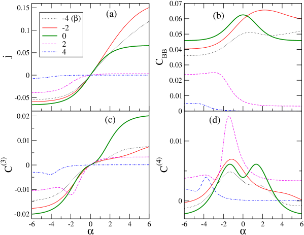
Figure 1: (Color online) First four cumulants of the current distribution as a function of $\alpha$, for 5 values of the interaction “strength” $\beta$ (see the legend). Note that for $\beta=0$ (SEP) odd cumulants are antisymmetric functions of the driving, while even cumulants are symmetric functions. This is due to a particle-hole symmetry, which is lost for interacting particles.

The mean current $j$ as a function of $\alpha$ and for several $\beta$’s is shown in figure 1(a). For a given $\beta$, $j$ increases with $\alpha$, linearly around $\alpha=0$, as expected close to equilibrium. For each $\alpha>0$ the mean current is maximal for a repulsive interaction ($\beta<0$), see the two examples in figure 2(a)). In general, the mean current $j$ is not antisymmetric with respect to $\alpha$, and its value in $\alpha$ can be very different from $-j$ in $-\alpha$.

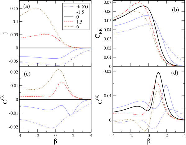
Figure 2: (Color online) First four cumulants of the current distribution as a function of $\beta$, for 5 values of the driving $\alpha$ (see the legend). Odd cumulants are identically zero when the system is in equilibrium ($\alpha=0$).

For $\beta\to-\infty$ the problem can be mapped into the dynamics of non-interacting dimers “$(0,1)$” and of $0$’s. In this limit the system is somewhat like a SEP with $1$’s replaced by dimers, and one thus expects a finite mean current. On the other hand, for $\beta\to+\infty$, particles stick together and it becomes more and more difficult for a hole (vacancy) to get in, to reach the bulk and finally to reach the other boundary of the channel. The hole essentially performs a random walk with an open left boundary before eventually reaching the system at the right boundary. If more than one hole enters into the system, there is a good chance that holes stick, further reducing the energy of the system, and their own mobility and $j$ as well. Thus, for $\beta\to\infty$ we expect $j\to 0$. These scenarios are qualitatively well confirmed in figure 2(a).

For $\beta=0$ one has the well-studied driven SEP. In this case the current is antisymmetric with $\alpha$, like all odd cumulants, because of a corresponding particle/hole symmetry.

3.2 Variance

The second cumulant of the current distribution is its variance. For $\beta=0$ the variance is symmetric with $\alpha$ (as every other even cumulant), while for all other cases it displays a non-trivial dependence on $\alpha$ and $\beta$, see figures 1(b) and 2(b). For $e^{\beta}\gg 1$ (see $\beta=4$ in figure 1(b)) the variance, as the current, can reach very small values, confirming the scenario proposed above.

3.3 Third and fourth cumulants

As for the current, for $\beta=0$ (SEP) the third cumulant of the current is antisymmetric with $\alpha$, see figure 1(c). In general, however, it is a complicated function of $\alpha$ and $\beta$, as evidenced by figure 2(c). For example, in contrast with the mean $j$, it can be a non-monotonous function of $\alpha$. Similar arguments apply to the fourth cumulant, see figure 1(d) and figure 2(d). The third and the fourth cumulant also appear going to zero for $e^{\beta}\gg 1$.

4 Traffic

Systematic perturbation techniques better be accompanied by a larger theoretical understanding. A major step in the analysis of the problem at hand that proceeds the numerical algorithm is contained in the simple path-distribution identity (8). On the left-hand side, this identity involves an average over paths $\omega$ in the original process, with probabilities $\operatorname{Prob}(\omega)$. The respective probabilities in the tilted space (with rates (6)) can be written as $\operatorname{Prob}_{\boldsymbol{\sigma}}(\omega)=e^{-Q(\omega)}\operatorname{Prob}(\omega)$, with relative path-space action $Q$. Since on the left-hand side of identity (8) we have a current generating function, a time-antisymmetric quantity is involved. On the other hand, on the right-hand side of (8) only a potential $V$ appears, i.e., a quantity depending only on the states and thus insensitive to time-reversal. Hence, the choice of the tilted Markov process is exactly such that the change in the time-antisymmetric part of the path-space action equals the appropriate sum over currents. This is why the exponent in the right-hand side of (8) contains a time-symmetric function only.

Such considerations are typical of the Lagrangian approach to nonequilibrium statistical mechanics as pioneered by Onsager and Machlup, ons . Here however we are not even close to equilibrium. We thus move on a somewhat generalized formalism that remains quite simple for finite state space Markov processes. Nevertheless the structure of time-symmetric versus time-antisymmetric fluctuations is possibly important for nonequilibrium thermodynamics, if only to identify the relevant thermodynamic potentials, cf. epl ; mnw1 ; mnw2 . Such an identification proceeds via a dynamical fluctuation theory, in which we next situate the main identity (8).

In order to rewrite (8) in another convenient form, we define occupation times as

$$\mu_{\eta}(\omega)=\frac{1}{T}\int_{0}^{T}\,\textrm{d}t\;\delta_{X_{t},\eta}$$

that the path $\omega=(X_{t},0<t\leq T)$ spends in state $\eta$. Then, the exponent in the right-hand side of (8) equals $\int_{0}^{T}V(X_{t})\,\textrm{d}t=T\sum_{\eta}V(\eta)\mu_{\eta}(\omega)$ or,

$$\langle e^{\sum_{B}\sigma_{B}J_{B}}\rangle=\langle e^{T\sum_{\eta}V(\eta)\mu_{\eta}}\rangle_{\boldsymbol{\sigma}}$$ (25)

The current statistics is therefore obtained when one knows the large deviation rate function $I^{\boldsymbol{\sigma}}$ for the occupation times,

$$\operatorname{Prob}_{\boldsymbol{\sigma}}[\mu_{\eta}\approx p(\eta),\forall\eta]\sim e^{-TI^{\boldsymbol{\sigma}}(p)},\quad T\uparrow+\infty$$

for the modified dynamics (6):

$$\lim_{T}\frac{1}{T}\log\langle e^{\sum_{B}\sigma_{B}J_{B}}\rangle=\sup_{\mu}(\mu\cdot V-I^{\boldsymbol{\sigma}}(\mu))$$ (26)

We have in mind here the application of the theory of large deviations as pioneered in DV for Markov processes.

In that last variational expression (26), the potential $V$ also depends on ${\boldsymbol{\sigma}}$. Let us introduce the antisymmetric form $\sigma(\eta,\xi)=\sigma_{B}$ for $(\eta,\xi)=b$ and $\sigma(\xi,\eta)=-\sigma(\eta,\xi)$. Then, the change (6) from the original rates $k(\eta,\xi)$ to the new rates $\ell(\eta,\xi)$ adds a further driving (in the spirit of local detailed balance): from (7), the term

$$\begin{split}\mu\cdot V&=\sum_{\eta}\mu(\eta)\,V(\eta)\\ &=\sum_{\eta}\mu(\eta)\,\sum_{\xi}k(\eta,\xi)[e^{\sigma(\eta,\xi)}-1]\\ &=\frac{1}{2}\sum_{\eta,\xi}[\tau_{\mu,\ell}(\eta,\xi)-\tau_{\mu,k}(\eta,\xi)]\end{split}$$ (27)

is an expected excess traffic, defined for rates $k$ as

$$\tau_{\mu,k}(\eta,\xi)=\mu(\eta)\,k(\eta,\xi)+\mu(\xi)\,k(\xi,\eta)$$

and similarly for rates $\ell$, see epl ; mnw1 ; mnw2 . The traffic expresses a time-symmetric kind of dynamical activity over the bond $b=(\eta,\xi)$. In fact, all cumulants of the expansion in Section 2.4 contain the term

$$n!\,{\langle\rho|}\;{\mathcal{L}}^{(n)}_{B}\;{|1\rangle}=\begin{cases}j_{B}&\text{for $n$ odd}\\ \tau_{B}&\text{for $n$ even}\end{cases}$$

with expected current over bonds $b\in B$

$$j_{B}={\langle\rho|}[E_{B}(0)-E_{-B}(0)]{|1\rangle}$$

and with corresponding expected traffic

$$\tau_{B}={\langle\rho|}[E_{B}(0)+E_{-B}(0)]{|1\rangle}$$

For instance, the first term on the right-hand-side of (16) is the stationary traffic $\tau_{B}$, while the second term can be interpreted as a zero-frequency autocorrelation function.

We stress that the traffic $\tau_{B}$ is symmetric under the exchange $\eta\leftrightarrow\xi$, while the current $j_{B}$ is antisymmetric. In other words, the traffic adds a time-symmetric aspect to the evaluation of the dynamical activity. Finally, note that the following identity holds,

$${\langle\rho|}{\mathcal{R}}{|1\rangle}=\sum_{B}\left[\tau_{B}\,(\cosh\sigma_{B}-1)+j_{B}\,\sinh\sigma_{B}\right]$$

Appendix A Markov generator and its normality

The operator $L$ that generates the Markov dynamics is a $M\times M$ matrix, and its spectral properties appear in the expansion for the cumulants (see more in the next appendix). It is important to realize some important changes with respect to equilibrium. For an equilibrium process with reversible distribution $\rho>0$ there is detailed balance,

$$\rho(\eta)\,L_{\eta\xi}=\rho(\xi)\,L_{\xi\eta}$$

Equivalently, the matrix

$$H_{\eta\xi}=\sqrt{\rho(\eta)}\,L_{\eta\xi}\,\frac{1}{\sqrt{\rho(\xi)}}$$

is then symmetric and hence diagonalizable with a complete orthonormal set of eigenvectors. The matrix $H$ is obtained from $L$ via a similarity transformation $H=Q^{-1}LQ$ with here, and that is essential, a diagonal similarity matrix $Q$. In other words, we easily find a scalar product for which the eigenvectors of a detailed balance generator are orthonormal. All that need not be possible for nonequilibrium processes.

A central notion here is that of normality: a matrix is normal if and only if it commutes with its adjoint if and only if it has a complete orthonormal set of eigenvectors. Detailed balance generators are similar with diagonal $Q$ to normal matrices while nonequilibrium processes have generators that need not be similar to normal matrices at all. When such a generator is similar to a normal matrix, then it is diagonalizable and we can work with a bi-orthogonal family of left/right eigenvectors. The following example illustrates some of these points.

Take the fully symmetric $3$-state Markov process, i.e. with all rates equal to 1, and perturb it obtaining the generator

$$\left(\begin{array}[]{ccc}-2-f+g&1+f&1-g\\ 1-f&-2+f-h&1+h\\ 1+g&1-h&-2-g+h\end{array}\right)$$

in the region $|f|,|g|,|h|<1$. The condition of detailed balance is satisfied on the surface $f+g+h+fgh=0$. The nature of the spectrum depends on the sign of $D=fg+fh+gh$: if $D<0$, then the generator is diagonalizable and has real eigenvalues; if $D=0$ and at least one of the $f,g$ or $h$ is non-zero, then the matrix is not diagonalizable; if $D>0$ then it is diagonalizable with complex eigenvalues. In particular, all three cases occur arbitrarily close to the reference equilibrium $f=g=h=0$.

One consequence of the above facts directly concerns the expansion and calculation of the cumulants following the scheme of Appendix B. We cannot simply rely on making use of some of the standard tools of quantum mechanical calculation, like decomposition in an orthonormal basis. An important example concerns the calculation of the pseudo-inverse as in (16)–(17). When we still have a decomposition of the unity in terms of left/right eigenvectors, then the pseudo-inverse ${G}$ can be obtained from

$${G}=({\mathbb{I}}-P)\frac{1}{L}({\mathbb{I}}-P)=\sum_{v=1}^{M-1}{|w_{v}^{(0)}\rangle}\frac{1}{e_{v}^{(0)}}{\langle\rho_{v}^{(0)}|}$$

with ${\langle\rho_{v}^{(0)}|}$ and ${|w_{v}^{(0)}\rangle}$ left and right eigenvectors of $L$ with eigenvalue $e_{v}^{(0)}<0$, and where

$$P\equiv{|1\rangle}{\langle\rho|}$$

is the projection on the vector space of constant functions (therefore ${\mathbb{I}}-P$ is the projection on the space orthogonal to them). In our general case, we employ the group inverse, a special case of Drazin inverse, see mey1 . Its role for the computational theory of Markov processes has been advocated in mey2 . The group inverse of $L$ is the unique solution ${G}$ of the equation

$$L\,{G}\,L=L,\quad{G}\,L\,{G}={G},\quad L\,{G}={G}\,L$$

As will appear in the next section, and as visible already in (16)–(17) and (19)–(20), that pseudo-inverse appears in the cumulant expansion.

A final important difference between symmetric versus non-symmetric matrices (up to a diagonal similarity transformation) concerns the application of a variational principle to characterize the maximal eigenvalue. For example, in quantum mechanics one usefully employs the Ritz variational principle for Hamiltonians (Hermitian matrices) and for finding the ground state energy. We are not aware of an extension of that Ritz variational method or of a more general minimax principle to non-Hermitian matrices. The only variational characterization that seems to remain goes undirectly via the relation of the largest eigenvalue to a suitable generating function, like in (12), which itself obtains a variational expression in terms of a large deviation rate function, like in formula (26).

Appendix B Rayleigh–Schrödinger expansion: the algorithm

We give a review of the expansion that is used to compute the leading orders in the maximal eigenvalue. We refer to pages 74–81 in the book of Kato Kato , for full details and for a rigorous treatment.

The RS expansion finds its origins in quantum mechanical problems of time-independent perturbation theory RSP1 ; RSP2 ; RSP3 . In contrast with the situation in quantum mechanics or with the case of detailed balance, we have in general no scalar product for which $L$ has an orthonormal basis of eigenvectors. In many cases in nonequilibrium, we do have a bi-orthogonal family of $M$ eigenvectors (instead of the orthonormal family in quantum mechanics) but it also happens that the generator is not diagonalizable and that we have no appropriate basis to express most easily the expansion. Fortunately, all that is not necessary and the expansion can proceed in a more general way. One simplifying feature is that the maximal eigenvalue that we need to compute is simple, as shown in Section 2.3. For the purpose of the present Appendix, we also make the simplification that only one $\sigma_{B}=\sigma\neq 0$.

The starting point is the $M\times M$ matrix $L+{\mathcal{R}}$ that we write in expansion

$${\mathcal{L}}=L+{\mathcal{R}}=\sum_{k=0}^{\infty}\sigma^{k}{\mathcal{L}}^{(k)},\qquad{\mathcal{L}}^{(0)}=L$$ (28)

The unperturbed generator $L$ has a resolvent $r(\kappa)=(L-\kappa)^{-1}$ with Laurent series around $\kappa=0$ given by

$$\frac{1}{L-\kappa}=-\frac{1}{\kappa}\,P+\sum_{m=0}\kappa^{m}{{G}}^{m+1}$$ (29)

for the projection $P={|1\rangle}\;{\langle\rho|}$ on the eigenspace of eigenvalue zero, and ${G}$ the pseudo-inverse in the sense of Drazin as we had in the previous section.

The resolvent for ${\mathcal{L}}$ is

$$r(\sigma,\kappa)=\frac{1}{{\mathcal{L}}-\kappa}$$

defined for all $\kappa$ not equal to any of the eigenvalues of ${\mathcal{L}}$. It can be written as a power series in $\sigma$ around (29):

$$r(\sigma,\kappa)=r(\kappa)+\sum_{n=1}^{+\infty}\sigma^{n}\,r^{(n)}(\kappa)$$ (30)

with

$$r^{(n)}(\kappa)=\sum_{\nu_{1}+\ldots+\nu_{p}=n}(-1)^{p}r(\kappa){\mathcal{L}}^{(\nu_{1})}r(\kappa){\mathcal{L}}^{(\nu_{2})}\ldots{\mathcal{L}}^{(\nu_{p})}r(\kappa)$$

where the sum is over all $1\leq p\leq n,\nu_{i}\geq 1$. On the other hand, by Cauchy’s residue theorem

$$e(\sigma)=-\frac{1}{2\pi i}\operatorname{Tr}\oint_{\Gamma}\kappa\,r(\sigma,\kappa)\,\textrm{d}\kappa$$ (31)

for a circle $\Gamma$ enclosing zero but no other eigenvalues of $L$. Upon substituting (30) into (31) we obtain

$$e(\sigma)=-\frac{1}{2\pi i}\operatorname{Tr}\oint_{\Gamma}\kappa r(\kappa)\sum_{p=1}^{+\infty}\big{[}-{\mathcal{R}}\,r(\kappa)\big{]}^{p}\,\textrm{d}\kappa$$ (32)

where ${\mathcal{R}}$ of course depends on $\sigma$. Since $\frac{\textrm{d}}{\textrm{d}\kappa}r(\kappa)=r(\kappa)^{2}$, we have

$$\begin{split}\frac{\textrm{d}}{\textrm{d}\kappa}\big{[}{\mathcal{R}}\,r(\kappa)\big{]}^{p}=&{\mathcal{R}}\,r(\kappa)\ldots{\mathcal{R}}\,r(\kappa){\mathcal{R}}\,r(\kappa)^{2}\\ &+{\mathcal{R}}\,r(\kappa)\ldots{\mathcal{R}}\,r(\kappa)^{2}{\mathcal{R}}\,r(\kappa)\\ &+\ldots+{\mathcal{R}}\,r(\kappa)^{2}\ldots{\mathcal{R}}\,r(\kappa){\mathcal{R}}\,r(\kappa)\end{split}$$

Observe now that the trace and the integration commute so that (32) becomes

$$e(\sigma)=-\frac{1}{2\pi i}\operatorname{Tr}\oint_{\Gamma}\kappa\sum_{p=1}^{+\infty}\frac{1}{p}\frac{\textrm{d}}{\textrm{d}\kappa}\big{[}-{\mathcal{R}}\,r(\kappa)\big{]}^{p}\,\textrm{d}\kappa$$

and after integration by parts

$$e(\sigma)=\frac{1}{2\pi i}\operatorname{Tr}\oint_{\Gamma}\sum_{p=1}^{+\infty}\frac{1}{p}\big{[}-{\mathcal{R}}\,r(\kappa)\big{]}^{p}\,\textrm{d}\kappa$$

or

$$e(\sigma)=-\frac{1}{2\pi i}\operatorname{Tr}\oint_{\Gamma}\log\big{[}1+{\mathcal{R}}\,r(\kappa)\big{]}\,\textrm{d}\kappa$$ (33)

Expanding the logarithm with (28) makes the expansion of the maximal eigenvalue

$$e(\sigma)=\sum_{n=1}^{+\infty}\sigma^{n}e^{(n)}=\sum_{n=1}^{+\infty}\sigma^{n}\frac{C^{(n)}}{n!}$$ (34)

for

$$e^{(n)}=\frac{1}{2\pi i}\operatorname{Tr}\sum_{\nu_{1}+\ldots+\nu_{p}=n}\frac{(-1)^{p}}{p}\oint_{\Gamma}{\mathcal{L}}^{(\nu_{1})}r(\kappa)\ldots{\mathcal{L}}^{(\nu_{p})}r(\kappa)\,\textrm{d}\kappa$$ (35)

We finally substitute the series (29) and perform the integral again with the residue theorem to get the result

$$e^{(n)}=\sum_{p=1}^{n}\frac{(-1)^{p}}{p}\sum_{\begin{subarray}{c}\nu_{1}+\ldots+\nu_{p}=n\\ k_{1}+\ldots+k_{p}=p-1\end{subarray}}\operatorname{Tr}{\mathcal{L}}^{(\nu_{1})}S^{(k_{1})}\ldots{\mathcal{L}}^{(\nu_{p})}S^{(k_{p})}$$ (36)

where $S^{(0)}=-P$ and $S^{(k)}={G}^{k}$. The last formula can be written more explicitly obtaining the different orders $C^{(n)}=n!\,e^{(n)}$ as in Section 2.4. As an example, let us show how to compute the cumulant of order $n=2$. The possible cases in the first sum of (36) are then $p=1$ and $p=2$.

For $p=1$ the second sum can only have $\nu_{1}=2$ and $k_{1}=0$, hence the contribution is $-\operatorname{Tr}{\mathcal{L}}^{(2)}S^{(0)}$. It is convenient to use the cyclic property of the trace operator $\operatorname{Tr}AB=\operatorname{Tr}BA$, and the definition $S^{(0)}=-P$ to rewrite the term as $\operatorname{Tr}P{\mathcal{L}}^{(2)}$. In general, given a set of left eigenvectors ${\langle\rho_{\ell}|}$ and right eigenvectors ${|w_{\ell}\rangle}$, for the trace one has $\operatorname{Tr}A=\sum_{\ell}{\langle\rho_{\ell}|}A{|w_{\ell}\rangle}$. Here, the projection $P$ on the $0$-th eigenvectors (${\langle\rho|}$ and ${|1\rangle}$) simplifies this term to ${\langle\rho|}{\mathcal{L}}^{(2)}{|1\rangle}$.

The only combinations of two numbers summing up to $p=2$ is $(\nu_{1}=1,\nu_{2}=1)$, while there are two choices $(k_{1}=1,k_{2}=0)$ and $(k_{1}=0,k_{2}=1)$ summing up to $p-1=1$. The former case corresponds to ${1\over 2}\operatorname{Tr}{\mathcal{L}}^{(1)}S^{(1)}{\mathcal{L}}^{(1)}S^{(0)}$ $={1\over 2}\operatorname{Tr}{\mathcal{L}}^{(1)}G{\mathcal{L}}^{(1)}(-P)$ $={1\over 2}\operatorname{Tr}-P{\mathcal{L}}^{(1)}G{\mathcal{L}}^{(1)}$, which is equal, according to previous arguments, to $-{1\over 2}{\langle\rho|}{\mathcal{L}}^{(1)}G{\mathcal{L}}^{(1)}{|1\rangle}$. The same is true for the second term ${1\over 2}\operatorname{Tr}{\mathcal{L}}^{(1)}S^{(0)}{\mathcal{L}}^{(1)}S^{(1)}$, and their sum cancels the factor $1/2$. Hence, overall one has the second cumulant given in Eq. (16).

Appendix C Numerical scheme

We have shown that all that is required for the computation of cumulants, regardless of their order, is the information on the stationary distribution ${\langle\rho|}$ and on the group inverse of the generator, i.e. the matrix ${G}$. An efficient computation of ${G}$ thus enables really making use of our formulas for the cumulants, like in Eq’s.(15)-(17), (19), and (20). Given $G$ and $\rho$, each cumulant is computed just by some matrix multiplications. The estimate of the group inverse of a generator $L$ is discussed in section 5 of mey2 and in sonin . In the computations carried out in this work, it turned out that

$${G}=P+(L-P)^{-1}$$

was the most stable way of computing ${G}$ for all parameter values. This formula derives most conveniently by using the properties of the so called fundamental matrix, see heyman .

However, for systems with a large number of degrees of freedom, it is rarely a good idea to directly invert matrices. Fortunately, it is also not necessary here. Note that any vector ${|z\rangle}=G{|y\rangle}$ coincides with the (unique) solution of the equation $L{|z\rangle}=({\mathbb{I}}-P){|y\rangle}$ constrained by the condition ${\langle{\rho}|{z}\rangle}=0$, as immediately follows from observing that $LG=GL={\mathbb{I}}-P$ and ${\langle\rho|}G=0$. Hence, objects like $GL^{(1)}GL^{(1)}{|1\rangle}$ or $G^{2}L^{(2)}{|1\rangle}$ can most conveniently be determined by solving a linear system of $M$ equations with subsequently updated right-hand side. The number of such linear problems is fixed by the order of cumulants to be computed. This formulation also invites an application of fast iterative methods and various schemes to store sparse matrices in the memory, which enable to remarkably increase the system size.

The second basic ingredient of the proposed algorithm is the computation of the stationary distribution ${\langle\rho|}$, for which one can choose among the available algorithms on the market. A possibility is to implement an Arnoldi scheme: the iteration of ${\langle\rho_{i+1}|}\leftarrow{\langle\rho_{i}|}(L+c{\mathbb{I}})$ converges to the eigenvector of $(L+c{\mathbb{I}})$ with largest modulus, which coincides with ${\langle\rho|}$ if the real constant $c>0$ is larger than the modulus of all eigenvalues of $L$.

Let us finally stress that the estimates of cumulants obtained in this paper, besides having their own theoretical interest, have the advantage of avoiding the use of finite differences, in this case of eigenvalues of $L_{\boldsymbol{\sigma}}$ obtained at different values of the parameters ${\boldsymbol{\sigma}}$. Like it is convenient to estimate the specific heat of a system from the variance of the energy distribution rather than from finite differences of the energy at different temperatures, we avoid the calculation of derivatives from finite differences, also because they usually hide dangerous dependencies on parameter step-sizes and the numerical instability connected with this. The latter is expected to be particularly problematic for cumulants of higher order.

References

- (1) Bustamante, C., Liphardt, J., Ritort, F.: Thermodynamics of small systems. Phys. Today pp. 43–48 (2005, July)
- (2) Rubi, J.M.: Non-equilibrium thermodynamics of small-scale systems. Energy 32, 297–300 (2007)
- (3) Saraniti, M., Ravaioli, U. (eds.): Nonequilibrium Carrier Dynamics in Semiconductors, Proceedings of the 14th International Conference (2005), Chicago, USA. Springer Proceedings in Physics, Berlin–Heidelberg (2005)
- (4) Blanter, Y.M., Büttiker, M.: Shot noise in mesoscopic conductors. Phys. Rep. 336(1), 1–166 (2000)
- (5) Nazarov, Y.V. (ed.): Quantum Noise in Mesoscopic Systems. Kluwer, Dordrecht (2003)
- (6) Jauho, A.P., Flindt, C., Novotny, T., Donarini, A.: Current and current fluctuations in quantum shuttles. Phys. Fluids 17, 10 (2005)
- (7) Flindt, C., Novotny, T., Jauho, A.P.: Full counting statistics of nano-electromechanical systems. Europhys. Lett. 69, 475–481 (2005)
- (8) Lee, H., Levitov, L.S., Yakovets, A.Y.: Universal statistics of transport in disordered conductors. Phys. Rev. B 51, 4079 – 4083 (1995)
- (9) Heikkilä, T.T., Ojanen, T.: Quantum detectors for the third cumulant of current fluctuations. Phys. Rev. B 75, 035,335 (2007)
- (10) Fujisawa, T., Hayashi, T., Tomita, R., Hirayama, Y.: Biderectional counting of singe electrons. Science 312, 1634 (2006)
- (11) Kurzynski, M.: The Thermodynamic Machinery of Life. Springer, Berlin (2005)
- (12) Haw, M.: The industry of life. Phys. World 20, 25–30 (2007)
- (13) Dellago, C., Geissler, P.L. (eds.): Monte Carlo sampling in path space: Calculating time correlation functions by transforming ensembles of trajectories, Proceedings of ”The Monte Carlo Method in the Physical Sciences: Celebrating the 50th anniversary of the Metropolis algorithm”, vol. 690. AIP Conference Proceedings (2003)
- (14) Dellago, C., Posch, H.A. (eds.): Realizing Boltzmann’s dream: computer simulations in modern statistical mechanics, Proceedings of the ESI conference ”Boltzmann’s legacy”. in print (2007)
- (15) Jarzynski, C.: Nonequilibrium equality for free energy differences. Phys. Rev. Lett. 78, 2690–2693 (1997)
- (16) Crooks, G.E.: Nonequilibrium measurements of free energy differences for microscopically reversible Markovian systems. J. Stat. Phys. 90, 1481–1487 (1998)
- (17) Evans, D.J., Cohen, E.G.D., Morriss, G.P.: Probability of second law violations in shearing steady flows. Phys. Rev. Lett. 71, 2401–2404 (1993)
- (18) Gallavotti, G., Cohen, E.G.D.: Dynamical ensembles in nonequilibrium statistical mechanics. Phys. Rev. Lett. 74, 2694–2697 (1995)
- (19) Gallavotti, G., Cohen, E.G.D.: Dynamical ensembles in stationary states. J. Stat. Phys. 80, 931–970 (1995)
- (20) Kurchan, J.: Fluctuation theorem for stochastic dynamics. J. Phys. A 31, 3719–3729 (1998)
- (21) Lebowitz, J., Spohn, H.: A Gallavotti–Cohen type symmetry in large deviation functional for stochastic dynamics. J. Stat. Phys. 95, 333–365 (1999)
- (22) Maes, C.: On the origin and the use of fluctuation relations for the entropy. Sémin. Poincaré 2, 29–62 (2003)
- (23) Maes, C., Netočný, K.: Time-reversal and entropy. J. Stat. Phys. 110, 269–310 (2003)
- (24) Keldysh, L.V.: Soviet Physics - JETP 20, 1018 (1965)
- (25) Craig, R.A.: J. Math. Phys. 9, 605 (1968)
- (26) Flindt, C., Novotny, T., Braggio, A., Sassetti, M., Jauho, A.: Counting statistics of non-Markovian quantum stochastic processes. Phys. Rev. Lett. 100, 150,601 (2008)
- (27) Pilgram, S., Jordan, A.N., Sukhorukov, E.V., Büttiker, M.: Stochastic path integral formulation of full counting statistics. Phys. Rev. Lett. 90, 206,801 (2003)
- (28) Kindermann, M., Trauzettel, B.: Current fluctuations of an interacting quantum dot. Phys. Rev. Lett. 94, 166,803 (2005)
- (29) Gershon, G., Bomze, Y., Sukhorukov, E.V., Reznikov, M.: Detection of non-Gaussian fluctuations in a quantum point contact. Phys. Rev. Lett. 101, 016,803 (2008)
- (30) Schmidt, T.L., Komnik, A., Gogolin, A.O.: Full counting statistics of spin transfer through ultrasmall quantum dots. Phys. Rev. B 76, 241,307(R) (2007)
- (31) Roche, P., Derrida, B., Doucot, B.: Mesoscopic full counting statistics and exclusion models. Eur. Phys. J. B 43, 529–541 (2005)
- (32) Bodineau, T., Derrida, B.: Current fluctuations in nonequilibrium diffusive systems: An additivity principle. Phys. Rev. Lett. 92, 180,601 (2004)
- (33) Bodineau, T., Derrida, B.: Distribution of current in nonequilibrium diffusive systems and phase transitions. Phys. Rev. E 72, 066,110 (2005)
- (34) Bertini, L., Sole, A.D., Jona-Lasinio, D.G.G., Landim, C.: Current fluctuations in stochastic lattice gases. Phys. Rev. Lett. 94, 030,601 (2005)
- (35) Bertini, L., Sole, A.D., Jona-Lasinio, D.G.G., Landim, C.: Non equilibrium current fluctuations in stochastic lattice gases. J. Stat. Phys. 123, 237–276 (2006)
- (36) Bodineau, T., Derrida, B.: Cumulants and large deviations of the current through non-equilibrium steady states. Comptes Rendus Physique 8, 540–555 (2007)
- (37) Appert-Rolland, C., B.Derrida, Lecomte, V., Van Wijland, F.: Universal cumulants of the current in diffusive systems on a ring (2008). ArXiv:0804.2590v1
- (38) Mehl, J., Speck, T., Seifert, U.: Large deviation function for entropy production in driven one-dimensional systems (2008). ArXiv:0804.0346v1
- (39) Giardinà, C., Kurchan, J., Peliti, L.: Direct evaluation of large-deviation functions. Phys. Rev. Lett. 96, 120,603 (2006)
- (40) Lecomte, V., J.Tailleur: A numerical approach to large deviations in continuous time. J. Stat. Mech. p. P03004 (2007)
- (41) Ràkos, A., Harris, R.J.: On the range of validity of the fluctuation theorem for stochastic Markovian dynamics. J. Stat. Mech. p. P05005 (2008)
- (42) Meyer, C.: Matrix Analysis and Applied Linear Algebra. SIAM (2000)
- (43) Maes, C., Netočný, K.: The canonical structure of dynamical fluctuations in mesoscopic nonequilibrium steady states. Europhys. Lett. 82, 30,003 (2008)
- (44) Maes, C., Netočný, K., Wynants, B.: Steady state statistics of driven diffusions. Physica A 387, 2675–2689 (2008)
- (45) Maes, C., Netočný, K., Wynants, B.: On and beyond entropy production: the case of Markov jump processes (2008). Markov Proc. Rel. Fields 14, 445–464 (2008)
- (46) Lecomte, V., Appert-Rolland, C., F. Van Wijland: Thermodynamic formalism and large deviation functions in continuous time Markov dynamics. Comptes Rendus Physique 8, 609–619 (2007)
- (47) Kipnis, C., Landim, C.: Scaling Limits of Interacting Particle Systems. Springer (1998)
- (48) B. Derrida, B.D., Roche, P.E.: Current fluctuations in the one-dimensional symmetric exclusion process with open boundaries. J. Stat. Phys. 115, 717–748 (2004)
- (49) Bodineau, T., Derrida, B.: Current large deviations for asymmetric exclusion processes with open boundaries. J. Stat. Phys. 123, 277–300 (2006)
- (50) Harris, R.J., Rákos, A., Schütz, G.M.: Current fluctuations in the zero-range process with open boundaries. J. Stat. Mech. p. P08003 (2005)
- (51) van Wijland, F., Rácz, Z.: Large deviations in weakly interacting boundary driven lattice gases. J. Stat. Phys. 118, 27–54 (2005)
- (52) Derrida, B., Lebowitz, J.L., Speer, E.R.: Free energy functional for nonequilibrium systems: An exactly soluble case. Phys. Rev. Lett. 87, 150,601 (2001)
- (53) Bertini, L., Sole, A.D., Jona-Lasinio, D.G.G., Landim, C.: Large deviations for the boundary driven symmetric simple exclusion process. Math. Phys., Analys. Geom. 6, 231–267 (2003)
- (54) Onsager, L., Machlup, S.: Fluctuations and irreversible processes. Phys. Rev. Lett. 91, 1505–1512 (1953)
- (55) Donsker, M.D., Varadhan, S.R.: Asymptotic evaluation of certain Markov process expectations for large time, I. Comm. Pure Appl. Math. 28, 1–47 (1975)
- (56) Meyer, C.D.: The riole of the group generalized inverse in the theory of finite Markov chains. SIAM Review 17, 443–464 (1975)
- (57) Sonin, I., Thornton, J.: Recursive algorithm for the fundamental/group inverse matrix of a Markov chain from an explicit formula. SIAM J. Matrix Analys. Applic. 23, 209–224 (2001)
- (58) Heyman, D.P.: Accurate computation of the fundamental matrix of a Markov chain. SIAM J. Matrix Analys. Applic. 16, 954–963 (1995)
- (59) Kato, T.: Perturbation Theory for Linear Operators, 2nd edition. Springer (1995)
- (60) Rayleigh, J.W.S.: Theory of Sound, 2nd edition, Vol. I, pp. 115–118. Macmillan, London (1894)
- (61) Schrödinger, E.: Annalen der Physik, Vierte Folge 80, 437 (1926)
- (62) Landau, L.D., Lifschitz, E.M.: Quantum Mechanics: Non-relativistic Theory, 3rd Ed. Butterworth-Heinemann (1981)