Exciton many-body effects through infinite series of composite-exciton operators

Abstract

We revisit the approach proposed by Mukamel and coworkers to describe interacting excitons through infinite series of composite-boson operators for both, the system Hamiltonian and the exciton commutator — which, in this approach, is properly kept different from its elementary boson value. Instead of free electron-hole operators, as used by Mukamel’s group, we here work with composite-exciton operators which are physically relevant operators for excited semiconductors. This allows us to get all terms of these infinite series explicitly, the first terms of each series agreeing with the ones obtained by Mukamel’s group when written with electron-hole pairs. All these terms nicely read in terms of Pauli and interaction scatterings of the composite-exciton many-body theory we have recently proposed. However, even if knowledge of these infinite series now allows to tackle $N$-body problems, not just 2-body problems like third order nonlinear susceptibility $\chi^{(3)}$, the necessary handling of these two infinite series makes this approach far more complicated than the one we have developed and which barely relies on just four commutators.

PACS number: 71.35.-y

1 Introduction

Most particles known as bosons, are composite particles made of even number of fermions. Proper treatment of the underlying Pauli exclusion principle between fermionic components of these particles has been a longstanding problem for decades [1]. Because many-body theories for quantum particles were, up to our work, valid for elementary particles only [2], sophisticated “bosonization” procedures [3,4] have been proposed to replace composite bosons by elementary bosons. These elementary bosons then interact through effective scatterings constructed on interactions which exist between their fermionic components, but dressed by “appropriate” fermion exchanges [5]. Although quite popular due to the fact that they allow calculations on problems otherwise unsolvable through known procedures, such bosonizations have an intrinsic major failure linked to the fact that, by replacing two free fermions by one boson, we strongly reduce degrees of freedom of the system. This shows up through the fact that, while closure relation for $N$ elementary bosons is

$$\bar{I}=\frac{1}{N!}\sum\bar{B}_{i_{1}}^{\dagger}\ldots\bar{B}_{i_{N}}^{\dagger}|v\rangle\,\langle v|\bar{B}_{i_{N}}\ldots\bar{B}_{i_{1}}\ ,$$ (1.1)

with $[\bar{B}_{i},\bar{B}_{j}]=\delta_{ij}$, the one for $N$ composite bosons made of two free fermions reads [6]

$$I=\frac{1}{(N!)^{2}}\sum B_{i_{1}}^{\dagger}\ldots B_{i_{N}}^{\dagger}|v\rangle\,\langle v|B_{i_{N}}\ldots B_{i_{1}}\ .$$ (1.2)

The huge prefactor change from $N!$ to $(N!)^{2}$ makes all sum rules for elementary and composite bosons, based on this closure relation, irretrievably different whatever are effective scatterings produced by bosonization procedures. And indeed, through this prefactor difference in closure relations, we have explained [6] the factor 1/2 difference in the link between lifetime and sum of transition rates that we had found [7] for composite and bosonized excitons.

Besides bosonization, very few other approaches to interacting composite bosons have been proposed. In the late 60’s, M. Girardeau [8] suggested to introduce a set of “ideal atom operators” in addition to fermionic operators for electrons and protons. These operators, which are bosonic by construction, represent all bound states of one atom, but not its extended states. They are forced into the problem through a so-called Fock-Tani unitary transformation which, in an exact way, transforms one exact atom bound state into one ideal-atom state. Unfortunately, this nicely simple result does not hold for $N$-atom states with $N\geq 2$, the procedure turning quite complicated very fast. This is why, although not advocated by Girardeau, we can be tempted by using his procedure as a bosonization procedure, i.e., by only keeping ideal-atom operators in transformed states and transformed Hamiltonian. We have however shown [9] that, with such a reduction, the obtained results for a few relevant physical quantities are at odd from the correct ones, even for the sign. The idea to add to fermionic operators for electrons and protons, a set of bosonic operators for atomic bound states, is in fact rather awkward because fermionic operators form a complete set in themselves; so that Girardeau artificially introduces an overcomplete set of operators in a problem already complex, this overcompleteness being obviously difficult to handle properly. Precise comparison of Girardeau’s procedure with the composite-boson many-body theory we have constructed, can be found in reference [9].

Another approach, still currently used [10-12], has been proposed by Mukamel and coworkers in the 90’s. It is based on the fully correct idea that the system Hamiltonian, when acting on fermion pairs, can be replaced by an infinite series of pair operators. In this approach, the fact that pairs of fermions differ from elementary bosons is kept exactly through commutators of pair operators which are also written as infinite series. The pair-operators used by Mukamel and coworkers are products of free fermion operators. However, as these are not physically relevant pair operators for problems dealing with excitons, their calculations turn out very complicated. This is probably why they have only derived the first term of the Hamiltonian and pair-commutator series. This thus makes their results of possible use for problems restricted to two excitons only. And indeed, using them, they have successfully calculated [12] the third order susceptibility $\chi^{(3)}$ which results from interactions of two unabsorbed photons through their coupling to two virtual excitons.

In this paper, we follow Mukamel and coworkers’ idea, but with exciton operators $B_{i}^{\dagger}$ instead of products of free-electron and free-hole operators $a_{\mathbf{k}_{e}}^{\dagger}b_{\mathbf{k}_{h}}^{\dagger}$, these exciton operators being the ones which create one-electron-hole-pair eigenstates of the system Hamiltonian,

$$(H-E_{i})B_{i}^{\dagger}|v\rangle=0\ .$$ (1.3)

Thanks to the closure relation for $N$ composite excitons, Eq.(1.2), it is easy to derive all terms of the series for the composite-boson commutator and for the system Hamiltonian in an exact way. As expected, prefactors in these infinite series read in terms of the two key parameters of the composite-boson many-body physics, namely Pauli scatterings for fermion exchanges in the absence of fermion interaction, and interaction scatterings for fermion interactions in the absence of fermion exchange.

However, even with these two infinite series at hand explicitly, so that problems dealing with many-body effects between $N$ excitons could now be tackled, this approach turns out to be definitely far more complicated than the composite-boson many-body theory we have recently constructed [13,14]. Indeed, in this new theory, calculations dealing with many-body effects between any number $N$ of excitons simply reduce to performing a set of commutations between exciton operators, according to two commutators for fermion exchanges (see Eq.(5) in ref. [15] or Eq. (14) in ref. [13]), namely,

$$[B_{m},B_{i}^{{\dagger}N}]=NB_{i}^{{\dagger}N-1}(\delta_{m,i}-D_{mi})-N(N-1)B_{i}^{{\dagger}N-2}\sum_{n}\lambda\left({}^{n\ \,i}_{m\ i}\right)B_{n}^{\dagger}\ ,$$ (1.4)

$$[D_{mi},B_{j}^{{\dagger}N}]=NB_{j}^{{\dagger}N-1}\sum_{n}\left\{\lambda\left({}^{n\ \,j}_{m\ i}\right)+\lambda\left({}^{m\ j}_{n\ \,i}\right)\right\}B_{n}^{\dagger}\ ,$$ (1.5)

and two commutators for fermion interactions (see Eq.(5) in ref. [16 ] or Eq.(13) in ref.[13]), namely,

$$[H,B_{i}^{{\dagger}N}]=NB_{i}^{{\dagger}N-1}(E_{i}B_{i}^{\dagger}+V_{i}^{\dagger})+\frac{N(N-1)}{2}B_{i}^{{\dagger}N-1}\sum_{m,n}\xi\left({}^{n\ \,i}_{m\ i}\right)B_{m}^{\dagger}B_{n}^{\dagger}\ ,$$ (1.6)

$$[V_{i}^{\dagger},B_{j}^{{\dagger}N}]=NB_{j}^{{\dagger}N-1}\sum_{m,n}\xi\left({}^{n\ \,j}_{m\ i}\right)B_{m}^{\dagger}B_{n}^{\dagger}\ .$$ (1.7)

In these equations, $D_{mi}$ is the exciton “deviation-from-boson operator” defined through Eq.(1.4) taken for $N=1$, namely,

$$D_{mi}=\delta_{m,i}-[B_{m},B_{i}^{\dagger}]\ ,$$ (1.8)

while Pauli scattering $\lambda\left({}^{n\ \,j}_{m\ i}\right)$ of two “in” excitons $(i,j)$ towards two “out” excitons $(m,n)$ follows from Eq.(1.5) taken for $N=1$ (also see Eq.(4) in ref.[17]), namely,

$$[D_{mi},B_{j}^{\dagger}]=\sum_{n}\left\{\lambda\left({}^{n\ \,j}_{m\ i}\right)+\lambda\left({}^{m\ j}_{n\ \,i}\right)\right\}B_{n}^{\dagger}\ .$$ (1.9)

In the same way, “creation potential” $V_{i}^{\dagger}$ of exciton $i$ and interaction scattering $\xi\left({}^{n\ \,j}_{m\ i}\right)$ follow from Eqs.(1.6) and (1.7) taken for $N=1$ (also see Eq.(3) in ref.[17]), namely,

$$[H,B_{i}^{\dagger}]=E_{i}B_{i}^{\dagger}+V_{i}^{\dagger}\ ,$$ (1.10)

$$[V_{i}^{\dagger},B_{j}^{\dagger}]=\sum_{m,n}\xi\left({}^{n\ \,i}_{m\ i}\right)B_{m}^{\dagger}B_{n}^{\dagger}\ .$$ (1.11)

Let us note that Eq.(1.8) which basically says that particles are not elementary but composite bosons, was known for quite a long time [1,18]. Equation (1.10) is more recent. It was introduced by one of us in her theory of exciton optical Stark effect [19,20]. On the contrary, Eqs.(1.9) and (1.11) which allow to reach the two elementary scatterings of two excitons, namely, $\lambda\left({}^{n\ \,j}_{m\ i}\right)$ and $\xi\left({}^{n\ \,j}_{m\ i}\right)$, are fundamentally new. They are the keys of our composite-boson many-body theory [17].

In this paper, we are going to use these four commutators to write the system Hamiltonian $H$ and the deviation-from-boson operator $D_{mi}$ as infinite series of exciton operators $B_{i}^{\dagger}$. This will allow us to generate physically relevant prefactors for these series. They are found to read in terms of exciton energies $E_{i}$, interaction scattering of two excitons $\xi\left({}^{n\ \,j}_{m\ i}\right)$, and the following sum of Pauli scatterings,

$$\Lambda_{mi}(n,j) = \lambda\left({}^{n\ \,j}_{m\ i}\right)+\lambda\left({}^{m\ j}_{n\ \,i}\right)$$ (1.12)

$$= \lambda_{e}\left({}^{n\ \,j}_{m\ i}\right)+\lambda_{h}\left({}^{n\ \,j}_{m\ i}\right)\ .$$

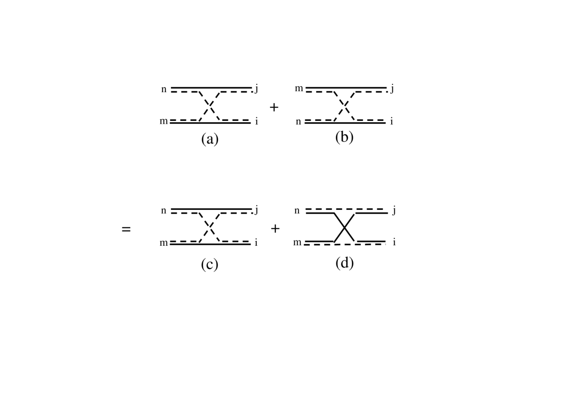
Figure 1: Shiva diagrams for $\Lambda_{mi}(n,j)$ defined in Eq.(1.12). $\lambda\left({}^{n\ \,j}_{m\ i}\right)$, represented by diagram (a), is identical to $\lambda_{e}\left({}^{n\ \,j}_{m\ i}\right)$, represented by diagram (c), in which $m$ and $i$ have the same electron. $\lambda\left({}^{m\ j}_{n\ \,i}\right)$, represented by diagram (b), is identical to $\lambda_{h}\left({}^{n\ \,j}_{m\ i}\right)$, represented by diagram (d), in which $m$ and $i$ have the same hole.

$\Lambda_{mi}(n,j)$, shown in Fig.1, corresponds to processes in which excitons $(i,j)$ exchange either a hole or an electron, excitons $(m,i)$ having same electron in $\lambda_{e}\equiv\lambda$, while they have same hole in $\lambda_{h}$: Due to electron-hole symmetry, it is quite reasonable to find these two processes on the same footing, in the $\Lambda_{mi}(n,j)$ factor.

2 Deviation-from-boson operator

Let us start with deviation-from-boson operator $D_{mi}$ defined in Eq.(1.8). Since both, $D_{mi}$ and the product of exciton operators $B_{m}^{\dagger}B_{i}$ conserve number of pairs, we can look for $D_{mi}$ as

$$D_{mi}=\sum_{n=1}^{\infty}D_{mi}^{(n)}\ ,$$ (2.1)

where the most general form for $D_{mi}^{(n)}$ acting in the subspace made of states having $p\geq n$ pairs, can be taken as

$$D_{mi}^{(n)}=\sum_{\{r\}}d_{mi}^{(n)}(r^{\prime}_{1},\ldots,r^{\prime}_{n};r_{1},\ldots,r_{n})B_{r^{\prime}_{1}}^{\dagger}\ldots B_{r^{\prime}_{n}}^{\dagger}B_{r_{1}}\ldots B_{r_{n}}\ .$$ (2.2)

We get this series by enforcing it to be such that, when acting on any $N$-exciton state $|\psi_{N}\rangle$ linear combination of $B_{j_{1}}^{\dagger}\ldots B_{j_{N}}^{\dagger}|v\rangle$, it gives the same result as the original operator $D_{mi}$, namely,

$$D_{mi}|\psi_{N}\rangle=\sum_{n=1}^{N}D_{mi}^{(n)}|\psi_{N}\rangle\ ,$$ (2.3)

for any $N$-pair state $|\psi_{N}\rangle$. We are going to derive the various operators $D_{mi}^{(n)}$ by iteration, starting from $n=1$, as we now show.

Before going further, it is of importance to note that, due to carrier exchanges between two excitons, we do have (see Eq.(5) in ref. [17])

$$B_{i}^{\dagger}B_{j}^{\dagger}=-\sum_{m,n}\lambda\left({}^{n\ \,j}_{m\ i}\right)B_{m}^{\dagger}B_{n}^{\dagger}\ .$$ (2.4)

This equation, which comes from the two ways to construct two excitons out of two electron-hole pairs, shows that $N$-exciton states $|\psi_{N}\rangle$ for $N\geq 2$, as well as operators like $D_{mi}^{(n)}$ for $n\geq 2$ can be written in many different ways, these various forms being related through the replacement of any $B^{\dagger}B^{\dagger}$ by a sum of $B^{\dagger}B^{\dagger}$ according to Eq.(2.4): Just as $B_{i_{1}}^{\dagger}\ldots B_{i_{N}}^{\dagger}|v\rangle$ states form an overcomplete set for $N$-pair states, $B_{i}^{\dagger}$’s form an overcomplete set of operators. This, in particular, allows us to guess that, among the various possible forms of $D_{mi}^{(n)}$, the one which has a physically relevant meaning, is most probably the simplest one. We will come back to this fundamental indetermination, linked to exciton composite nature, at the end of this section.

2.1 Derivation of $D_{mi}^{(1)}$

Let us first consider a one-exciton state $|\psi_{1}\rangle$. By inserting closure relation for one-exciton subspace , i.e., Eq.(1.2) taken for $N=1$, in front of this state, we find

$$D_{mi}|\psi_{1}\rangle=\sum_{r_{1}}D_{mi}B_{r_{1}}^{\dagger}|v\rangle\langle v|B_{r_{1}}|\psi_{1}\rangle\ .$$ (2.5)

As $D_{mi}B_{r_{1}}^{\dagger}|v\rangle=[D_{mi},B_{r_{1}}^{\dagger}]|v\rangle$ since $D_{mi}|v\rangle=0$ which follows from Eq.(1.8) acting on vacuum, we get from Eqs.(1.9,12)

$$D_{mi}|\psi_{1}\rangle=\sum_{r^{\prime}_{1},r_{1}}\Lambda_{mi}(r^{\prime}_{1},r_{1})B_{r^{\prime}_{1}}^{\dagger}|v\rangle\langle v|B_{r_{1}}|\psi_{1}\rangle\ ,$$ (2.6)

where $\Lambda_{mi}(n,j)$ is the combination of Pauli scatterings introduced in Eq.(1.12).

We then note that projector $|v\rangle\langle v|$ can be removed from this equation since state $B_{r_{1}}|\psi_{1}\rangle$ has zero pair while identity operator reduces to $|v\rangle\langle v|$ for such a state. Consequently, Eq.(2.6) also reads

$$D_{mi}|\psi_{1}\rangle=\sum_{r^{\prime}_{1},r_{1}}\Lambda_{mi}(r^{\prime}_{1},r_{1})B_{r^{\prime}_{1}}^{\dagger}B_{r_{1}}|\psi_{1}\rangle\ .$$ (2.7)

Since this equation is valid for any state $|\psi_{1}\rangle$, we readily find that operator $D_{mi}^{(1)}$ such that $D_{mi}|\psi_{1}\rangle=D_{mi}^{(1)}|\psi_{1}\rangle$ can be taken as

$$D_{mi}^{(1)}=\sum_{r^{\prime}_{1},r_{1}}\Lambda_{mi}(r^{\prime}_{1},r_{1})B_{r^{\prime}_{1}}^{\dagger}B_{r_{1}}\ ,$$ (2.8)

with $\Lambda_{mi}(r^{\prime}_{1},r_{1})$ given in Eq.(1.12). This result is the same as the one given by Mukamel and coworkers (see Eqs. (11-13) of Ref.[12]).

2.2 Derivation of $D_{mi}^{(2)}$

We now consider two-exciton state $|\psi_{2}\rangle$. By inserting closure relation, Eq.(1.2), for two-exciton subspace, in front of $|\psi_{2}\rangle$, we get

$$D_{mi}|\psi_{2}\rangle=\left(\frac{1}{2!}\right)^{2}\sum_{r_{1},r_{2}}D_{mi}B_{r_{1}}^{\dagger}B_{r_{2}}^{\dagger}|v\rangle\langle v|B_{r_{2}}B_{r_{1}}|\psi_{2}\rangle\ .$$ (2.9)

To go further, we note that, due to Eqs.(1.9) and (1.12),

$$D_{mi}B_{r_{1}}^{\dagger}B_{r_{2}}^{\dagger}|v\rangle = \left([D_{mi},B_{r_{1}}^{\dagger}]+B_{r_{1}}^{\dagger}D_{mi}\right)B_{r_{2}}^{\dagger}|v\rangle$$ (2.10)

$$= \sum_{r^{\prime}}B_{r^{\prime}}^{\dagger}\left(\Lambda_{mi}(r^{\prime},r_{1})B_{r_{2}}^{\dagger}+\Lambda_{mi}(r^{\prime},r_{2})B_{r_{1}}^{\dagger}\right)|v\rangle\ .$$

We then insert this result into Eq.(2.9) and relabel bold indices. By noting that projector $|v\rangle\langle v|$ can again be removed from this equation since $B_{r_{2}}B_{r_{1}}|\psi_{2}\rangle$ also has zero pair, we end with

$$D_{mi}|\psi_{2}\rangle=\frac{2}{(2!)^{2}}\sum_{r^{\prime}_{1},r_{1},r_{2}}\Lambda_{mi}(r^{\prime}_{1},r_{1})B_{r^{\prime}_{1}}^{\dagger}B_{r_{2}}^{\dagger}B_{r_{2}}B_{r_{1}}|\psi_{2}\rangle\ .$$ (2.11)

If we now turn to $D_{mi}^{(1)}$ acting on $|\psi_{2}\rangle$, we note that $B_{r_{1}}|\psi_{2}\rangle$ has one pair so that, if we insert closure relation for one-pair subspace in front of this state, we find

$$D_{mi}^{(1)}|\psi_{2}\rangle=\sum_{r^{\prime}_{1},r_{1}}\Lambda_{mi}(r^{\prime}_{1},r_{1})B_{r^{\prime}_{1}}^{\dagger}\left[\sum_{r_{2}}B_{r_{2}}^{\dagger}|v\rangle\langle v|B_{r_{2}}\right]B_{r_{1}}|\psi_{2}\rangle\ .$$ (2.12)

We can again remove projector $|v\rangle\langle v|$ from this equation since $B_{r_{2}}B_{r_{1}}|\psi_{2}\rangle$ has zero pair. This readily shows that operator $D_{mi}^{(2)}$ such that $D_{mi}|\psi_{2}\rangle=\left(D_{mi}^{(1)}+D_{mi}^{(2)}\right)|\psi_{2}\rangle$ can be taken as

$$D_{mi}^{(2)}=-\frac{1}{2}\sum_{r^{\prime}_{1},r_{1},r_{2}}\Lambda_{mi}(r^{\prime}_{1},r_{1})B_{r^{\prime}_{1}}^{\dagger}B_{r_{2}}^{\dagger}B_{r_{2}}B_{r_{1}}\ .$$ (2.13)

2.3 Derivation of $D_{mi}^{(3)}$

To better grasp how $D_{mi}^{(n)}$ can be constructed by iteration, let us calculate one more $D_{mi}^{(n)}$ explicitly. We consider three-pair state $|\psi_{3}\rangle$ and inject in front of it, closure relation for three-pair subspace. This leads to

$$D_{mi}|\psi_{3}\rangle=\frac{1}{(3!)^{2}}\sum_{r_{1},r_{2},r_{3}}D_{mi}B_{r_{1}}^{\dagger}B_{r_{2}}^{\dagger}B_{r_{3}}^{\dagger}|v\rangle\langle v|B_{r_{3}}B_{r_{2}}B_{r_{1}}|\psi_{3}\rangle\ .$$ (2.14)

To go further, we do like for Eq.(2.10) and use commutator $[D_{mi},B_{r}^{\dagger}]$ given in Eq.(1.9). This leads to

$$D_{mi}B_{r_{1}}^{\dagger}B_{r_{2}}^{\dagger}B_{r_{3}}^{\dagger}|v\rangle=\sum_{r^{\prime}}\left\{\Lambda_{mi}(r^{\prime},r_{1})B_{r_{2}}^{\dagger}B_{r_{3}}^{\dagger}+\Lambda_{mi}(r^{\prime},r_{2})B_{r_{1}}^{\dagger}B_{r_{3}}^{\dagger}\right.$$

$$\left.+\Lambda_{mi}(r^{\prime},r_{3})B_{r_{1}}^{\dagger}B_{r_{2}}^{\dagger}\right\}|v\rangle\ .$$ (2.15)

We then inject this result into Eq.(2.14), relabel bold indices and remove projector $|v\rangle\langle v|$. This leads to

$$D_{mi}|\psi_{3}\rangle=\frac{3}{(3!)^{2}}\sum_{r^{\prime}_{1},\{r\}}\Lambda_{mi}(r^{\prime}_{1},r_{1})B_{r^{\prime}_{1}}^{\dagger}B_{r_{2}}^{\dagger}B_{r_{3}}^{\dagger}B_{r_{3}}B_{r_{2}}B_{r_{1}}|\psi_{3}\rangle\ .$$ (2.16)

We now turn to $D_{mi}^{(1)}|\psi_{3}\rangle$. Since $B_{r_{1}}|\psi_{3}\rangle$ has two pairs, we get, by using closure relation for two-pair subspace,

$$D_{mi}^{(1)}|\psi_{3}\rangle=\left(\frac{1}{2!}\right)^{2}\sum_{r^{\prime}_{1},\{r\}}\Lambda_{mi}(r^{\prime}_{1},r_{1})B_{r^{\prime}_{1}}^{\dagger}B_{r_{2}}^{\dagger}B_{r_{3}}^{\dagger}\mathbf{\rangle}\langle v|B_{r_{3}}B_{r_{2}}B_{r_{1}}|\psi_{3}\rangle\ .$$ (2.17)

We do the same for $D_{mi}^{(2)}|\psi_{3}\rangle$ in which $B_{r_{1}}B_{r_{2}}|\psi_{3}\rangle$ has one pair. By collecting all terms, we see that operator $D_{mi}^{(3)}$ such that $D_{mi}|\psi_{3}\rangle=\left(D_{mi}^{(1)}+D_{mi}^{(2)}+D_{mi}^{(3)}\right)|\psi_{3}\rangle$ can be taken as

$$D_{mi}^{(3)}=\frac{1}{3}\sum_{r^{\prime}_{1},\{r\}}\Lambda_{mi}(r^{\prime}_{1},r_{1})B_{r^{\prime}_{1}}^{\dagger}B_{r_{2}}^{\dagger}B_{r_{3}}^{\dagger}B_{r_{3}}B_{r_{2}}B_{r_{1}}\ .$$ (2.18)

2.4 Derivation of $D_{mi}^{(n)}$

The above results lead us to think that operator $D_{mi}^{(n)}$ can be written as

$$D_{mi}^{(n)}=\gamma_{n}\sum_{r^{\prime}_{1},\{r\}}\Lambda_{mi}(r^{\prime}_{1},r_{1})B_{r^{\prime}_{1}}^{\dagger}B_{r_{2}}^{\dagger}\ldots B_{r_{n}}^{\dagger}B_{r_{n}}\ldots B_{r_{2}}B_{r_{1}}\ ,$$ (2.19)

where $\gamma_{n}$ is a numerical prefactor which, in spite of its values for $n=(1,2,3)$, does not reduce to $(-1)^{n-1}/n$.

To determine $\gamma_{n}$, we look for the recursion relation it obeys. To get this recursion relation, we follow the procedure we have used for $n\leq 3$, namely, we insert closure relation for $N$-pair subspace in front of state $|\psi_{N}\rangle$. This leads to

$$D_{mi}|\psi_{N}\rangle=\left(\frac{1}{N!}\right)^{2}\sum_{\{r\}}D_{mi}B_{r_{1}}^{\dagger}\ldots B_{r_{N}}^{\dagger}|v\rangle\langle v|B_{r_{N}}\ldots B_{r_{1}}|\psi_{N}\rangle\ .$$ (2.20)

We then calculate $D_{mi}B_{r_{1}}^{\dagger}\ldots B_{r_{N}}^{\dagger}|v\rangle$ using commutator (1.9); we relabel bold indices and remove projector $|v\rangle\langle v|$. This gives

$$D_{mi}|\psi_{N}\rangle=\frac{N}{(N!)^{2}}\sum_{r^{\prime}_{1},\{r\}}\Lambda_{mi}(r^{\prime}_{1},r_{1})B_{r^{\prime}_{1}}^{\dagger}B_{r_{2}}^{\dagger}\ldots B_{r_{N}}^{\dagger}B_{r_{N}}\ldots B_{r_{2}}B_{r_{1}}|\psi_{N}\rangle\ .$$ (2.21)

We then turn to $D_{mi}^{(n)}$ acting on $|\psi_{N}\rangle$ for $n<N$. Since state $B_{r_{1}}\ldots B_{r_{n}}|\psi_{N}\rangle$ has $(N-n)$ pairs, closure relation for this subspace leads to

$$D_{mi}^{(n)}|\psi_{N}\rangle=\left(\frac{1}{(N-n)!}\right)^{2}\gamma_{n}\sum_{r^{\prime}_{1},\{r\}}\Lambda_{mi}(r^{\prime}_{1},r_{1})B_{r^{\prime}_{1}}^{\dagger}B_{r_{2}}^{\dagger}\ldots B_{r_{n}}B_{r_{n+1}}^{\dagger}\ldots B_{r_{N}}^{\dagger}$$

$$\times\ B_{r_{N}}\ldots B_{r_{n+1}}B_{r_{n}}\ldots B_{r_{1}}|\psi_{N}\rangle\ .$$ (2.22)

By inserting these results into Eq.(2.3), it is easy to show that the form Eq.(2.19) for $D_{mi}^{(n)}$ is indeed valid provided that $\gamma_{n}$’s are linked by

$$\gamma_{N}=\frac{N}{(N!)^{2}}-\sum_{n=1}^{N-1}\frac{\gamma_{n}}{[(N-n)!]^{2}}\ ,$$ (2.23)

with $\gamma_{1}=1$. From this equation, it is easy to show that the first $\gamma_{n}$’s are

$$\gamma_{2} = -1/2$$

$$\gamma_{3} = 1/3$$

$$\gamma_{4} = -11/48$$

$$\gamma_{5} = 11/120\ ,$$ (2.24)

and so on…, with $\gamma_{N}$ going to zero with increasing $N$.

2.5 Other forms of $D_{mi}^{(n)}$

As said at the beginning of this section, composite-boson operators $B_{i}^{\dagger}$ form an overcomplete set to describe electron-hole pairs. This is why any given operator acting in $N$-pair subspace with $N\geq 2$, when written in terms of these $B_{i}^{\dagger}$’s, can appear through different expressions. Indeed, due to Eq.(2.4), it is possible to rewrite $B_{r^{\prime}_{1}}^{\dagger}B_{r_{2}}^{\dagger}$ in Eq.(2.19) as

$$B_{r^{\prime}_{1}}^{\dagger}B_{r_{2}}^{\dagger}=-\sum_{r^{\prime\prime}_{1},r^{\prime}_{2}}\lambda\left({}^{r^{\prime\prime}_{1}\ r_{2}}_{r^{\prime}_{2}\ \,r^{\prime}_{1}}\right)B_{r^{\prime\prime}_{1}}^{\dagger}B_{r^{\prime}_{2}}^{\dagger}\ ,$$ (2.25)

since $B_{m}^{\dagger}B_{n}^{\dagger}=B_{n}^{\dagger}B_{m}^{\dagger}$. We then note that

$$\sum_{r^{\prime}_{1}}\lambda\left({}^{r^{\prime\prime}_{1}\ r_{2}}_{r^{\prime}_{2}\ \,r^{\prime}_{1}}\right)\lambda\left({}^{r^{\prime}_{1}\ r_{1}}_{m\ \,i}\right)=\lambda_{3}\left(\begin{array}[]{ll}r^{\prime}_{2}&r_{2}\\ r^{\prime\prime}_{1}&r_{1}\\ m&i\end{array}\right)\ ,$$ (2.26)

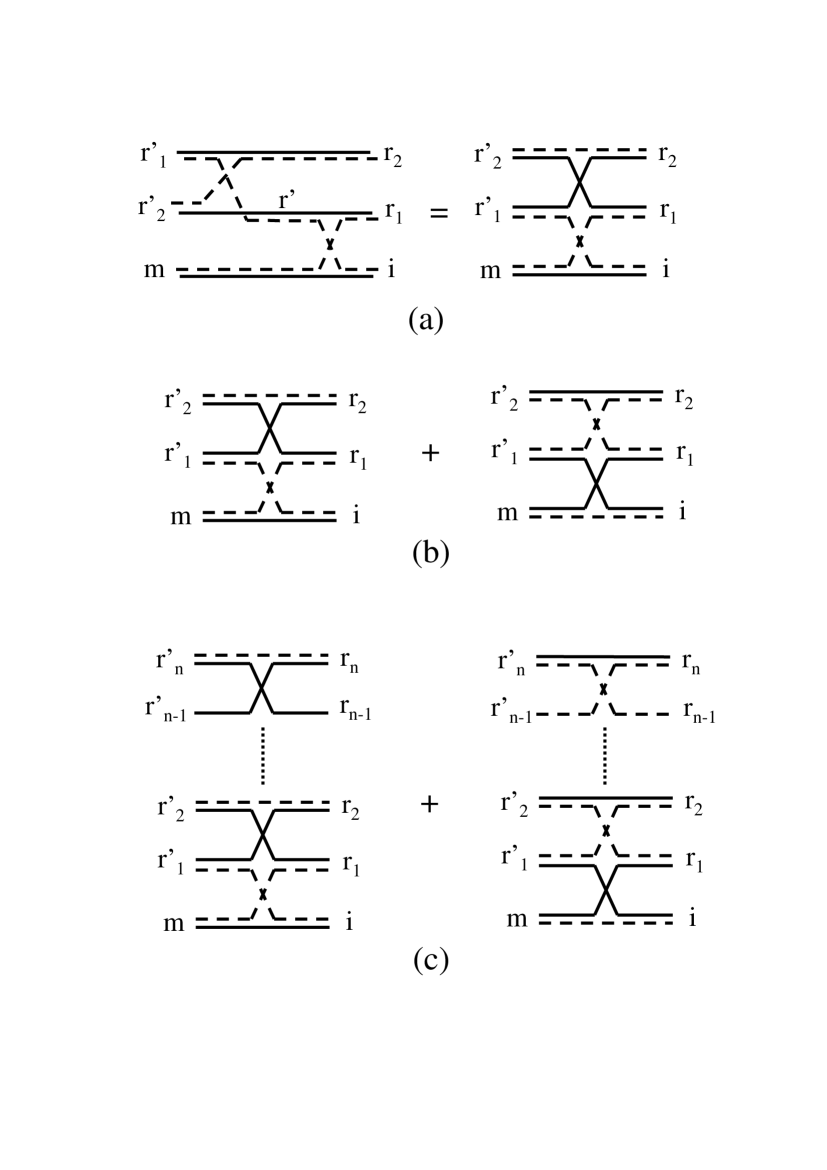
Figure 2: (a) Shiva diagram representation of Eq.(2.27), the summation over the bold index $r^{\prime}$ being performed readily. (b) Shiva diagrams for the prefactor $\Lambda_{mi}\left({}^{r^{\prime}_{2}\ r_{2}}_{r^{\prime}_{1}\ r_{1}}\right)$ appearing in Eq.(2.28). This prefactor corresponds to carrier exchanges between $(i,r_{1},r_{2})$ leading to $(m,r^{\prime}_{1},r^{\prime}_{2})$, in which the excitons $m$ and $i$ either have the same electron or the same hole. (c) Same as (b) for the prefactor appearing in Eq.(2.29).

where, according to Fig.2(a), $\lambda_{3}$ is just the exchange scattering between three excitons $(i,r_{1},r_{2})$. This allows us to replace the first factor of $D_{mi}^{(n)}$ in Eq.(2.19) by

$$\sum_{r^{\prime}_{1}}\Lambda_{mi}(r^{\prime}_{1},r_{1})B_{r^{\prime}_{1}}^{\dagger}B_{r_{2}}^{\dagger}=-\sum_{r^{\prime\prime}_{1},r^{\prime}_{2}}\Lambda_{mi}\left({}^{r^{\prime}_{2}\ r_{2}}_{r^{\prime\prime}_{1}\ r_{1}}\right)B_{r^{\prime\prime}_{1}}^{\dagger}B_{r^{\prime}_{2}}^{\dagger}\ .$$ (2.27)

While prefactor $\Lambda_{mi}(r^{\prime}_{1},r_{1})$ corresponds to carrier exchanges between two excitons $(i,r_{1})$ leading to $(m,r^{\prime}_{1})$ with excitons $m$ and $i$ having either same electron or same hole, prefactor $\Lambda_{mi}\left({}^{r^{\prime}_{2}\ r_{2}}_{r^{\prime\prime}_{1}\ r_{1}}\right)$ corresponds to carrier exchanges between excitons $(i,r_{1},r_{2})$ leading to $(m,r^{\prime\prime}_{1},r^{\prime}_{2})$, with excitons $m$ and $i$ also having either same electron or same hole (see Fig.2(b)).

If we keep doing this procedure for $B_{r^{\prime}_{2}}^{\dagger}B_{r_{3}}^{\dagger}$ with $B_{r^{\prime}_{2}}^{\dagger}$ relabelled as $B_{r^{\prime}_{1}}^{\dagger}$, and so on …, we end with $D_{mi}^{(n)}$ written in a quite symmetrical form, although far more complicated than Eq.(2.19), namely,

$$D_{mi}^{(n)}=(-1)^{n-1}\gamma_{n}\sum_{\{r^{\prime}\},\{r\}}\Lambda_{mi}\left(\begin{array}[]{ll}r^{\prime}_{n}&r_{n}\\ .&.\\ .&.\\ r^{\prime}_{1}&r_{1}\end{array}\right)B_{r^{\prime}_{1}}^{\dagger}\ldots B_{r^{\prime}_{n}}^{\dagger}B_{r_{n}}\ldots B_{r_{1}}\ ,$$ (2.28)

where the prefactor corresponds to carrier exchanges between $(n+1)$ excitons $(i,r_{1},\ldots,r_{n})$ leading to $(m,r^{\prime}_{1},\ldots,r^{\prime}_{n})$ in which excitons $m$ and $i$ either have same electron or same hole (see Fig.2(c)).

3 System Hamiltonian

Let us now turn to the system Hamiltonian originally written in terms of fermionic operators for free electrons and free holes. It contains kinetic electron and hole contributions. It also contains Coulomb interaction between electrons, between holes and between electrons and holes. It is actually quite easy to write the electron-hole part of this Hamiltonian in terms of excitons. Indeed, by using the link between exciton operators and free-electron and free-hole operators, namely,

$$B_{i}^{\dagger}=\sum_{\mathbf{k}_{e},\mathbf{k}_{h}}a_{\mathbf{k}_{e}}^{\dagger}b_{\mathbf{k}_{h}}^{\dagger}\langle\mathbf{k}_{h},\mathbf{k}_{e}|i\rangle\ ,$$ (3.1)

$$a_{\mathbf{k}_{e}}^{\dagger}b_{\mathbf{k}_{h}}^{\dagger}=\sum_{i}B_{i}^{\dagger}\langle i|\mathbf{k}_{e},\mathbf{k}_{h}\rangle\ ,$$ (3.2)

where $\langle\mathbf{k}_{h},\mathbf{k}_{e}|i\rangle$ is $i$ exciton wave function in momentum space, we readily find electron-hole Coulomb interaction as

$$V_{eh} = -\sum_{\mathbf{q},\mathbf{k}_{e},\mathbf{k}_{h}}V_{\mathbf{q}}a_{\mathbf{k}_{e}+\mathbf{q}}^{\dagger}b_{\mathbf{k}_{h}-\mathbf{q}}^{\dagger}b_{\mathbf{k}_{h}}a_{\mathbf{k}_{e}}$$ (3.3)

$$= -\sum_{i,j}B_{i}^{\dagger}B_{j}\sum_{\mathbf{q},\mathbf{k}_{e},\mathbf{k}_{h}}V_{\mathbf{q}}\langle i|\mathbf{k}_{e}+\mathbf{q},\mathbf{k}_{h}-\mathbf{q}\rangle\langle\mathbf{k}_{h},\mathbf{k}_{e}|j\rangle\ .$$

On the contrary, this cannot be done for other parts of the Hamiltonian, namely, kinetic energy terms in $a^{\dagger}a$ and $b^{\dagger}b$ and electron-electron and hole-hole Coulomb terms in $a^{\dagger}a^{\dagger}aa$ and $b^{\dagger}b^{\dagger}bb$. Nevertheless, since both operator $H$ and product of exciton operators $B_{m}^{\dagger}B_{i}$, conserve the number of electron-hole pairs, it is a priori possible to write $H$ as

$$H=\sum_{n=1}^{\infty}H^{(n)}\ ,$$ (3.4)

$$H^{(n)}=\sum_{\{r\},\{r^{\prime}\}}h^{(n)}(r^{\prime}_{1},\ldots,r^{\prime}_{n};r_{1},\ldots,r_{n})B_{r^{\prime}_{1}}^{\dagger}\ldots B_{r^{\prime}_{n}}^{\dagger}B_{r_{n}}\ldots B_{r_{1}}\ ,$$ (3.5)

so that $H^{(n)}$ acts on states having $p\geq n$ pairs. This series is determined by enforcing

$$H|\psi_{N}\rangle=\sum_{n=1}^{N}H^{(n)}|\psi_{N}\rangle\ ,$$ (3.6)

for any state $|\psi_{N}\rangle$ having $N$ electron-hole pairs. Here again, $H^{(n)}$ for $n\geq 2$ is expected to have various forms since any $B^{\dagger}B^{\dagger}$ can be replaced by sum of $B^{\dagger}B^{\dagger}$, according to Eq.(2.4). To get the various terms of $H^{(n)}$ expansion, we are again going to extensively use closure relation (1.2) for $N$-pair states. This will allow us to get one of these possible forms of $H$ quite easily.

3.1 Derivation of $H^{(1)}$

To get $H^{(1)}$, we insert closure relation for one-pair states in front of $|\psi_{1}\rangle$ in $H|\psi_{1}\rangle$. This leads to

$$H|\psi_{1}\rangle=\sum_{r_{1}}HB_{r_{1}}^{\dagger}|v\rangle\langle v|B_{r_{1}}|\psi_{1}\rangle\ .$$ (3.7)

We first replace $HB_{r_{1}}^{\dagger}|v\rangle$ by $E_{r_{1}}B_{r_{1}}^{\dagger}|v\rangle$ for exciton operators create one-pair eigenstates of the system. We then note that $B_{r_{1}}|\psi_{1}\rangle$ has zero pair, so that we can remove projector $|v\rangle\langle v|$ from this equation. This leads to

$$H|\psi_{1}\rangle=\sum_{r_{1}}E_{r_{1}}B_{r_{1}}^{\dagger}B_{r_{1}}|\psi_{1}\rangle\ .$$ (3.8)

Since $H^{(1)}|\psi_{1}\rangle$ must be equal to $H|\psi_{1}\rangle$ for any one-pair state $|\psi_{1}\rangle$, we readily see that $H^{(1)}$ can be identified with

$$H^{(1)}=\sum_{r_{1}}E_{r_{1}}B_{r_{1}}^{\dagger}B_{r_{1}}\ .$$ (3.9)

3.2 Derivation of $H^{(2)}$

We now turn to two-pair subspace. By inserting closure relation for two-pair states in front of $|\psi_{2}\rangle$, we find

$$H|\psi_{2}\rangle=\left(\frac{1}{2!}\right)^{2}\sum_{r_{1},r_{2}}HB_{r_{1}}^{\dagger}B_{r_{2}}^{\dagger}|v\rangle\langle v|B_{r_{2}}B_{r_{1}}|\psi_{2}\rangle\ .$$ (3.10)

We then use Eqs.(1.10,11) to find

$$HB_{r_{1}}^{\dagger}B_{r_{2}}^{\dagger}|v\rangle = (B_{r_{1}}^{\dagger}H+E_{r_{1}}B_{r_{1}}^{\dagger}+V_{r_{1}}^{\dagger})B_{r_{2}}^{\dagger}|v\rangle$$ (3.11)

$$= (E_{r_{1}}+E_{r_{2}})B_{r_{1}}^{\dagger}B_{r_{2}}^{\dagger}|v\rangle+\sum_{r^{\prime}_{1},r^{\prime}_{2}}\xi\left({}^{r^{\prime}_{2}\ r_{2}}_{r^{\prime}_{1}\ r_{1}}\right)B_{r^{\prime}_{1}}^{\dagger}B_{r^{\prime}_{2}}^{\dagger}|v\rangle\ .$$

If we insert this result into Eq.(3.10), relabel bold indices and remove projector $|v\rangle\langle v|$, we end with

$$H|\psi_{2}\rangle=\left(\frac{1}{2}\sum_{r_{1},r_{2}}E_{r_{1}}B_{r_{1}}^{\dagger}B_{r_{2}}^{\dagger}B_{r_{2}}B_{r_{1}}+\frac{1}{4}\sum_{r_{1},r_{2},r^{\prime}_{1},r^{\prime}_{2}}\xi\left({}^{r^{\prime}_{2}\ r_{2}}_{r^{\prime}_{1}\ r_{1}}\right)B_{r^{\prime}_{1}}^{\dagger}B_{r^{\prime}_{2}}B_{r_{2}}B_{r_{1}}\right)|\psi_{2}\rangle\ .$$ (3.12)

Let us now turn to $H^{(1)}$ acting on $|\psi_{1}\rangle$. We first note that $B_{r_{1}}|\psi_{2}\rangle$ has one pair so that closure relation for one-pair subspace leads to

$$H^{(1)}|\psi_{1}\rangle=\sum_{r_{1},r_{2}}E_{r_{1}}B_{r_{1}}^{\dagger}B_{r_{2}}^{\dagger}|v\rangle\langle v|B_{r_{2}}B_{r_{1}}|\psi_{1}\rangle\ ,$$ (3.13)

in which we can remove projector $|v\rangle\langle v|$ since $B_{r_{2}}B_{r_{1}}|\psi_{1}\rangle$ has zero pair.

This readily shows that $H^{(2)}$, such that $H\psi_{2}\rangle=\left(H^{(1)}+H^{(2)}\right)|\psi_{2}\rangle$, can be identified with

$$H^{(2)}=-\frac{1}{2}\sum_{r_{1},r_{2}}E_{r_{1}}B_{r_{1}}^{\dagger}B_{r_{2}}^{\dagger}B_{r_{2}}B_{r_{1}}+\frac{1}{4}\sum_{r^{\prime}_{1},r^{\prime}_{2},r_{1},r_{2}}\xi\left({}^{r^{\prime}_{2}\ r_{2}}_{r^{\prime}_{1}\ r_{1}}\right)B_{r^{\prime}_{1}}^{\dagger}B_{r^{\prime}_{2}}^{\dagger}B_{r_{2}}B_{r_{1}}\ .$$ (3.14)

3.3 Derivation of $H^{(3)}$

To grasp how series $H$ is constructed, let us calculate one more $H^{(n)}$ explicitly. From closure relation for 3-pair states, we find

$$H|\psi_{3}\rangle=\left(\frac{1}{3!}\right)^{2}\sum_{\{r\}}HB_{r_{1}}^{\dagger}B_{r_{2}}^{\dagger}B_{r_{3}}^{\dagger}|v\rangle\langle v|B_{r_{3}}B_{r_{2}}B_{r_{1}}|\psi_{3}\rangle\ .$$ (3.15)

We then use Eqs.(1.10,11) to find

$$HB_{r_{1}}^{\dagger}B_{r_{2}}^{\dagger}B_{r_{3}}^{\dagger}|v\rangle=(E_{r_{1}}+E_{r_{2}}+E_{r_{3}})B_{r_{1}}^{\dagger}B_{r_{2}}^{\dagger}B_{r_{3}}^{\dagger}|v\rangle+\sum_{s,t}B_{s}^{\dagger}B_{t}^{\dagger}\left[\xi\left({}^{t\ r_{2}}_{s\ r_{1}}\right)B_{r_{3}}^{\dagger}\right.$$

$$\left.\xi\left({}^{t\ r_{3}}_{s\ r_{2}}\right)B_{r_{1}}^{\dagger}+\xi\left({}^{t\ r_{1}}_{s\ r_{3}}\right)B_{r_{2}}^{\dagger}\right]\ .$$ (3.16)

So that, if we insert this result into Eq.(3.15), relabel bold indices and remove projector $|v\rangle\langle v|$, we end with

$$H|\psi_{3}\rangle=\left[\frac{3}{(3!)^{2}}\sum_{\{r\}}E_{r_{1}}B_{r_{1}}^{\dagger}B_{r_{2}}^{\dagger}B_{r_{3}}^{\dagger}B_{r_{3}}B_{r_{2}}B_{r_{1}}\right.\hskip 85.35826pt$$

$$\left.+\frac{C_{3}^{2}}{(3!)^{2}}\sum_{r^{\prime}_{1},r^{\prime}_{2},\{r\}}\xi\left({}^{r^{\prime}_{2}\ r_{2}}_{r^{\prime}_{1}\ r_{1}}\right)B_{r^{\prime}_{1}}^{\dagger}B_{r^{\prime}_{2}}^{\dagger}B_{r_{3}}^{\dagger}B_{r_{3}}B_{r_{2}}B_{r_{1}}\right]|\psi_{3}\rangle\ ,$$ (3.17)

where $C_{N}^{2}=N(N-1)/2$ is the number of ways we can choose 2 excitons among $N$. This makes $C_{3}^{2}=3$.

We now turn to $\left(H^{(1)}+H^{(2)}\right)|\psi_{3}\rangle$ that we calculate by injecting closure relations for 2-pair states in front of $B_{r_{1}}|\psi_{3}\rangle$ and for one-pair states in front of $B_{r_{1}}B_{r_{2}}|\psi_{3}\rangle$. By collecting all these results, we find that $H^{(3)}$ such that $H|\psi_{3}\rangle=\left(H^{(1)}+H^{(2)}+H^{(3)}\right)|\psi_{3}\rangle$ can be identified with

$$H^{(3)}=\frac{1}{3}\sum_{\{r\}}E_{r_{1}}B_{r_{1}}^{\dagger}B_{r_{2}}^{\dagger}B_{r_{3}}^{\dagger}B_{r_{3}}B_{r_{2}}B_{r_{1}}-\frac{1}{6}\sum_{r^{\prime}_{1},r^{\prime}_{2},\{r\}}\xi\left({}^{r^{\prime}_{2}\ r_{2}}_{r^{\prime}_{1}\ r_{1}}\right)B_{r^{\prime}_{1}}^{\dagger}B_{r^{\prime}_{2}}^{\dagger}B_{r_{3}}^{\dagger}B_{r_{3}}B_{r_{2}}B_{r_{1}}\ .$$ (3.18)

3.4 Derivation of $H^{(n)}$

The above results lead us to think that operator $H^{(n)}$ can be written as

$$H^{(n)}=\alpha_{n}\,\sum_{\{r\}}E_{r_{1}}B_{r_{1}}^{\dagger}\ldots B_{r_{n}}^{\dagger}B_{r_{n}}\ldots B_{r_{1}}\hskip 142.26378pt$$

$$+\beta_{n}\,\sum_{r^{\prime}_{1},r^{\prime}_{2},\{r\}}\xi\left({}^{r^{\prime}_{2}\ r_{2}}_{r^{\prime}_{1}\ r_{1}}\right)B_{r^{\prime}_{1}}^{\dagger}B_{r^{\prime}_{2}}^{\dagger}B_{r_{3}}^{\dagger}\ldots B_{r_{n}}^{\dagger}B_{r_{n}}\ldots B_{r_{1}}\ ,$$ (3.19)

with $\alpha_{n}=-2\beta_{n}=\gamma_{n}$ for $n>1$, with $\gamma_{n}$ being the prefactor appearing in $D_{mi}$ series (see Eq.(2.23)), while $(\alpha_{1}=1,\beta_{1}=0)$ for $n=1$.

In order to show this nicely simple result, we are going to determine the recursion relations which exist between $\alpha_{n}$’s and between $\beta_{n}$’s. For that, we follow the procedure we have previously used, namely, we first insert closure relation for the $N$-pair states in front of $|\psi_{N}\rangle$. This leads to

$$H|\psi_{N}\rangle=\frac{1}{(N!)^{2}}\sum_{\{r\}}HB_{r_{1}}^{\dagger}\ldots B_{r_{N}}^{\dagger}|v\rangle\langle v|B_{r_{N}}\ldots B_{r_{1}}|\psi_{N}\rangle\ .$$ (3.20)

We then calculate $H$ acting on $N$ excitons through Eq.(1.10). This leads to

$$HB_{r_{1}}^{\dagger}\ldots B_{r_{N}}^{\dagger}|v\rangle=(B_{r_{1}}^{\dagger}H+E_{r_{1}}B_{r_{1}}^{\dagger}+V_{r_{1}}^{\dagger})B_{r_{2}}^{\dagger}\ldots B_{r_{N}}^{\dagger}|v\rangle\ .$$ (3.21)

By using Eq.(1.11), we find

$$V_{r_{1}}^{\dagger}B_{r_{2}}^{\dagger}\ldots B_{r_{N}}^{\dagger}|v\rangle = \left([V_{r_{1}}^{\dagger},B_{r_{2}}^{\dagger}]+B_{r_{2}}^{\dagger}V_{r_{1}}^{\dagger}\right)B_{r_{3}}^{\dagger}\ldots B_{r_{N}}^{\dagger}|v\rangle$$ (3.22)

$$= \sum_{r^{\prime}_{1},r^{\prime}_{2}}\xi\left({}^{r^{\prime}_{2}\ r_{2}}_{r^{\prime}_{1}\ r_{1}}\right)B_{r^{\prime}_{1}}^{\dagger}B_{r^{\prime}_{2}}^{\dagger}B_{r_{3}}^{\dagger}\ldots B_{r_{N}}^{\dagger}|v\rangle+B_{r_{2}}^{\dagger}V_{r_{1}}^{\dagger}B_{r_{3}}^{\dagger}\ldots B_{r_{N}}^{\dagger}|v\rangle\ .$$

We iterate the procedure to end with

$$HB_{r_{1}}^{\dagger}\ldots B_{r_{N}}^{\dagger}|v\rangle=(E_{r_{1}}+\cdots+E_{r_{N}})B_{r_{1}}^{\dagger}\ldots B_{r_{N}}^{\dagger}|v\rangle\hskip 142.26378pt$$

$$+\left\{\sum_{r^{\prime}_{1},r^{\prime}_{2}}\xi\left({}^{r^{\prime}_{2}\ r_{2}}_{r^{\prime}_{1}\ r_{1}}\right)B_{r^{\prime}_{1}}^{\dagger}B_{r^{\prime}_{2}}^{\dagger}B_{r_{3}}^{\dagger}\ldots B_{r_{N}}^{\dagger}|v\rangle\ +\ \mathrm{permutations}\right\}\ ,$$ (3.23)

the total number of these $\xi$ terms being the number of ways $C_{N}^{2}$ we can choose among $N$, the two excitons having direct Coulomb process.

If we now relabel bold indices and remove projector $|v\rangle\langle v|$, we end with

$$H|\psi_{N}\rangle=\frac{N}{(N!)^{2}}\sum_{\{r\}}E_{r_{1}}B_{r_{1}}^{\dagger}\ldots B_{r_{N}}^{\dagger}B_{r_{N}}\ldots B_{r_{1}}|\psi_{N}\rangle\hskip 113.81102pt$$

$$+\frac{C_{N}^{2}}{(N!)^{2}}\sum_{r^{\prime}_{1},r^{\prime}_{2},\{r\}}\xi\left({}^{r^{\prime}_{2}\ r_{2}}_{r^{\prime}_{1}\ r_{1}}\right)B_{r^{\prime}_{1}}^{\dagger}B_{r^{\prime}_{2}}^{\dagger}B_{r_{3}}^{\dagger}\ldots B_{r_{N}}^{\dagger}B_{r_{N}}\ldots B_{r_{1}}|\psi_{N}\rangle\ .$$ (3.24)

We now turn to $H^{(n)}$ acting on $|\psi_{N}\rangle$ and assume that its general form is indeed given by Eq.(3.19). Since state $B_{r_{n}}\ldots B_{r_{1}}|\psi_{N}\rangle$ has $(N-n)$ pairs, we get, by injecting closure relation for $(N-n)$-pair subspace,

$$H^{(n)}|\psi_{N}\rangle=\frac{1}{((N-n)!)^{2}}\sum_{\{r\}}\left[\alpha_{n}E_{r_{1}}B_{r_{1}}^{\dagger}B_{r_{2}}^{\dagger}+\beta_{n}\sum_{r^{\prime}_{1},r^{\prime}_{2}}\xi\left({}^{r^{\prime}_{2}\ r_{2}}_{r^{\prime}_{1}\ r_{1}}\right)B_{r^{\prime}_{1}}^{\dagger}B_{r^{\prime}_{2}}^{\dagger}\right]$$

$$\times\ B_{r_{3}}^{\dagger}\ldots B_{r_{n}}^{\dagger}B_{r_{n+1}}^{\dagger}\ldots B_{r_{N}}^{\dagger}|v\rangle\langle v|B_{r_{N}}\ldots B_{r_{1}}|\psi_{N}\rangle\ .$$ (3.25)

We then remove projector $|v\rangle\langle v|$ as usual. By collecting all these results, we find that operator $H^{(n)}$ defined through Eq.(3.6) has the form (3.19) provided that $\alpha_{n}$’s and $\beta_{n}$’s are linked by

$$\alpha_{N}=\frac{N}{(N!)^{2}}-\sum_{n=1}^{N-1}\frac{\alpha_{n}}{((N-n)!)^{2}}\ ,$$ (3.26)

$$\beta_{N}=\frac{C_{N}^{2}}{(N!)^{2}}-\sum_{n=2}^{N-1}\frac{\beta_{n}}{((N-n)!)^{2}}\ ,$$ (3.27)

with $\alpha_{1}=1$ and $\beta_{1}=0$, due to Eq.(3.9), while $\beta_{2}=1/4$, due to Eq.(3.14). By comparing Eqs.(2.23) and (3.26), we readily see that $\alpha_{N}=\gamma_{N}$. In order to determine $\beta_{N}$, we first note that the recursion relation for $\alpha_{N}$ also reads

$$\alpha_{N} = \frac{N}{(N!)^{2}}-\frac{1}{((N-1)!)^{2}}-\sum_{n=2}^{N-1}\frac{\alpha_{n}}{((N-n)!)^{2}}$$ (3.28)

$$= -\frac{N(N-1)}{(N!)^{2}}-\sum_{n=2}^{N-1}\frac{\alpha_{n}}{((N-n)!)^{2}}\ .$$

Since $C_{N}^{2}=N(N-1)/2$, this equation is nothing but the recursion relation for $\beta_{N}$ provided that we replace $\alpha_{N}$ by $(-2\beta_{N})$ for any $N\geq 2$. Consequently, we end with

$$\gamma_{N}=\alpha_{N}=-2\beta_{N}\ \ \mathrm{for}\ \ N\geq 2\ ,$$ (3.29)

while $\alpha_{1}=\gamma_{1}=1$ and $\beta_{1}=0$, in agreement with our original guess.

4 Discussion

4.1 Summary of the results

The above results lead us to write deviation-from-boson operator $D_{mi}$ of two composite excitons defined as

$$[B_{m},B_{i}^{\dagger}]=\delta_{m,i}-D_{mi}\ ,$$ (4.1)

through an infinite series of exciton-operator products, according to

$$D_{mi}=\sum_{r^{\prime},r}\left[\lambda\left({}^{r^{\prime}\ \,r}_{m\ i}\right)+\lambda\left({}^{m\ r}_{r^{\prime}\ \,i}\right)\right]B_{r^{\prime}}^{\dagger}\left(1+\sum_{n=2}^{\infty}\gamma_{n}P_{n}\right)B_{r}\ ,$$ (4.2)

$$P_{n}=\sum_{\{j\}}B_{j_{1}}^{\dagger}\ldots B_{j_{n-1}}^{\dagger}B_{j_{n-1}}\ldots B_{j_{1}}\ .$$ (4.3)

$\lambda\left({}^{r^{\prime}\ \,r}_{m\ i}\right)$ is the Pauli scattering for carrier exchanges between “in” excitons $(i,r)$ leading to “out” excitons $(m,r^{\prime})$, with excitons $(m,i)$ having same electron. Electron-hole symmetry is restored through the fact that, in the second term of Eq.(4.2), namely, $\lambda\left({}^{m\ r}_{r^{\prime}\ \,i}\right)$, excitons $(m,i)$ have same hole (see Fig.1).

$\gamma_{n}$’s are numerical prefactors which obey the recursion relation

$$\gamma_{N}=\frac{N}{(N!)^{2}}-\sum_{n=1}^{N-1}\frac{\gamma_{n}}{((N-n)!)^{2}}\ ,$$ (4.4)

with $\gamma_{1}=1$; so that $\gamma_{2}=-1/2$, $\gamma_{3}=1/3$, and so on…, with $\gamma_{N}$ going to zero for increasing $N$.

In the same way, the system Hamiltonian, when acting on electron-hole-pair states, can be written as an infinite series of exciton-operator products, according to

$$H=\sum_{r}E_{r}B_{r}^{\dagger}\left(1+\sum_{n=2}^{\infty}\gamma_{n}P_{n}\right)B_{r}\hskip 227.62204pt$$

$$+\frac{1}{2}\sum_{r_{1},r_{2},r^{\prime}_{1},r^{\prime}_{2}}\xi\left({}^{r^{\prime}_{2}\ r_{2}}_{r^{\prime}_{1}\ r_{1}}\right)B_{r^{\prime}_{1}}^{\dagger}B_{r^{\prime}_{2}}^{\dagger}\left(\frac{1}{2}-\sum_{n=3}^{\infty}\gamma_{n}P_{n-1}\right)B_{r_{2}}B_{r_{1}}\ .$$ (4.5)

Let us again stress that, since there are two ways to form two excitons out of two electron-hole pairs, any product $B^{\dagger}B^{\dagger}$ can be written as a sum of $B^{\dagger}B^{\dagger}$ according to Eq.(2.4). Consequently, it is always possible to rewrite sums appearing in $D_{mi}$ and $H$ in various different ways, Eqs.(4.2-5) being the simplest ones.

4.2 Comparison with Mukamel and coworkers’ results

In their works, Mukamel and coworkers use free-pair operators $\hat{B}_{m}^{\dagger}=c_{m_{1}}^{\dagger}d_{m_{2}}^{\dagger}$, where $c_{m_{1}}^{\dagger}$ creates electron on site $m_{1}$ while $d_{m_{2}}^{\dagger}$ creates hole on site $m_{2}$. The fact that they use sites while we here use momenta (see Eq.(3.2)) is basically unimportant. They however keep the possibility for electrons and holes of these free pairs to differ from free Hamiltonian eigenstates. This is why they have nondiagonal contributions in the one-body part of their Hamiltonian,

$$H_{0}=\sum_{m_{1},n_{1}}t^{(1)}_{m_{1}n_{1}}c_{m_{1}}^{\dagger}c_{n_{1}}+\sum_{m_{2},n_{2}}t^{(2)}_{m_{2}n_{2}}d_{m_{2}}^{\dagger}d_{n_{2}}\ .$$ (4.6)

As these free-pair states are not physically relevant states to describe a set of $N$ interacting pairs, Mukamel and coworkers only reach the two first terms of $H$ series, namely, $H^{(1)}$ and $H^{(2)}$, and the first term of $D_{mi}$ series, their results reading already as rather complicated (see Eq.(18) of ref.[10]). To make precise link with their work, we are going to recover their results from our compact forms.

As electron-hole states used by Mukamel and coworkers form complete set, we can expand exciton operators $B_{r}^{\dagger}$ in terms of electron-hole operators $\hat{B}_{n}^{\dagger}$, according to

$$B_{r}^{\dagger}=\sum_{n}\hat{B}_{n}^{\dagger}\langle\hat{n}|r\rangle\ ,$$ (4.7)

where $|r\rangle=B_{r}^{\dagger}|v\rangle$, while $|\hat{n}\rangle=\hat{B}_{n}^{\dagger}|v\rangle=c_{n_{1}}^{\dagger}d_{n_{2}}^{\dagger}|v\rangle$.

Using this expansion (4.7), we see that the first term of the $H$ series we have obtained, also reads

$$H^{(1)} = \sum_{r_{1}}E_{r_{1}}B_{r_{1}}^{\dagger}B_{r_{1}}$$ (4.8)

$$= \sum_{m,n}h_{mn}\hat{B}_{m}^{\dagger}\hat{B}_{n}\ ,$$

where prefactor $h_{mn}$ is nothing but

$$h_{mn}=\sum_{r_{1}}E_{r_{1}}\langle\hat{m}|r_{1}\rangle\langle r_{1}|\hat{n}\rangle=\langle\hat{m}|H|\hat{n}\rangle\ ,$$ (4.9)

since $H|r_{1}\rangle=E_{r_{1}}|r_{1}\rangle$. If we now introduce the two-body part of the Hamiltonian as written in Eq.(16) of ref.[10], namely,

$$H_{c}=\frac{1}{2}\sum V^{(1)}_{m_{1}n_{1}j_{1}k_{1}}c_{m_{1}}^{\dagger}c_{n_{1}}^{\dagger}c_{j_{1}}c_{k_{1}}+\frac{1}{2}\sum V^{(2)}_{m_{2}n_{2}j_{2}k_{2}}d_{m_{2}}^{\dagger}d_{n_{2}}^{\dagger}d_{j_{2}}d_{k_{2}}-\sum W_{m_{1}n_{2}j_{1}k_{2}}c_{m_{1}}^{\dagger}d_{n_{2}}^{\dagger}d_{j_{2}}c_{k_{1}}\ ,$$ (4.10)

we see that, for $H=H_{0}+H_{c}$ with $H_{0}$ given in Eq.(4.6), prefactor $h_{mn}$ defined in Eq.(4.9) splits as

$$h_{mn} = h_{mn}^{(0)}-W_{m_{1}m_{2}n_{1}n_{2}}$$

$$h_{mn}^{(0)} = t_{m_{1}n_{1}}^{(1)}\delta_{m_{2},n_{2}}+t_{m_{2}n_{2}}^{(2)}\delta_{m_{1},n_{1}}\ ,$$ (4.11)

in agreement with the result obtained by Mukamel and coworkers for the first term of $H$ expansion.

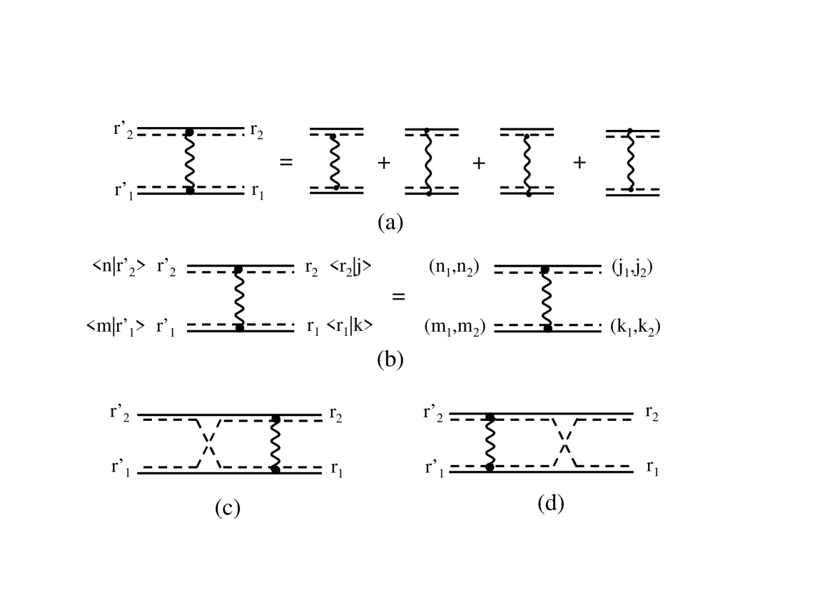
Figure 3: (a) Direct Coulomb scattering $\xi\left({}^{r^{\prime}_{2}\ r_{2}}_{r^{\prime}_{1}\ r_{1}}\right)$ between the “in” excitons $(r_{1},r_{2})$ leading to the “out” excitons $(r^{\prime}_{1},r^{\prime}_{2})$. This scattering is “direct” in the sense that the electron-hole pairs are coupled similarly in the “in” and “out” states. (b) Diagrammatic representation of the sum over $\{r\}$ appearing in Eq.(4.14) and leading to Eq.(4.15). (c) Shiva diagram representation for the “in” exchange Coulomb scattering $\xi^{\mathrm{in}}\left({}^{r^{\prime}_{2}\ r_{2}}_{r^{\prime}_{1}\ r_{1}}\right)$ defined in Eq.(4.22). In this scattering, the Coulomb interactions are between the “in” excitons. (d) Shiva diagram representation of the “out” exchange Coulomb scattering $\xi^{\mathrm{out}}\left({}^{r^{\prime}_{2}\ r_{2}}_{r^{\prime}_{1}\ r_{1}}\right)$ defined in Eq.(4.23). In this scattering, the Coulomb interactions are between the “out” excitons.

We now turn to $H^{(2)}$. In view of Eq.(3.14), $H^{(2)}$ splits as $H^{(2)}=H_{E}^{(2)}+H_{\xi}^{(2)}$, where $H_{E}^{(2)}$ depends on exciton energy $E_{r}$ while $H_{\xi}^{(2)}$ depends on exciton scattering $\xi$. Before going further, let us note that, since $H_{E}^{(2)}$ contains exciton energy $E_{r}$, this term, by construction, contains a part of electron-hole Coulomb interaction, namely, the one acting inside one exciton. On the other hand, as $H_{\xi}^{(2)}$ reads in terms of direct Coulomb scattering $\xi\left({}^{r^{\prime}_{2}\ r_{2}}_{r^{\prime}_{1}\ r_{1}}\right)$ between the two excitons $(r_{1},r_{2})$, it contains Coulomb scattering resulting from electron-electron and hole-hole interactions as well as from electron-hole interaction between excitons $r_{1}$ and $r_{2}$ (see Fig.3(a)). Since electron-hole interaction already appears in the first-order term $H^{(1)}$ through $W_{m_{1}m_{2}n_{1}n_{2}}$ in $h_{mn}$ (see Eq.(4.11)), these two electron-hole contributions of $H^{(2)}$ must somehow cancel, as we now show.

If we symmetrize $H_{E}^{(2)}$ and write exciton operators in terms of free pairs according to Eq.(4.7), we find

$$H_{E}^{(2)} = -\frac{1}{4}\sum_{r_{1},r_{2}}(E_{r_{1}}+E_{r_{2}})B_{r_{1}}^{\dagger}B_{r_{2}}^{\dagger}B_{r_{2}}B_{r_{1}}$$ (4.12)

$$= -\frac{1}{4}\sum_{m,n,j,k}\hat{B}_{m}^{\dagger}\hat{B}_{n}^{\dagger}\hat{B}_{j}\hat{B}_{k}\left[\sum_{r_{1}}\langle\hat{m}|H|r_{1}\rangle\langle r_{1}|\hat{k}\rangle\sum_{r_{2}}\langle\hat{n}|r_{2}\rangle\langle r_{2}|\hat{j}\rangle+\ (1\leftrightarrow 2)\right]\ .$$

Using Eq.(4.9) and orthogonality of free-pair states, we readily find

$$H_{E}^{(2)}=-\frac{1}{4}\sum_{m,n,j,k}\hat{B}_{m}^{\dagger}\hat{B}_{n}^{\dagger}\hat{B}_{j}\hat{B}_{k}(h_{mk}\delta_{n,j}+h_{nj}\delta_{m,k})\ ,$$ (4.13)

with $h_{mn}$ given in Eq.(4.11).

If we now consider the part of $H_{\xi}^{(2)}$ coming from Coulomb scattering $\xi$ between excitons, we can rewrite it, using again Eq.(4.7), as

$$H_{\xi}^{(2)} = \frac{1}{4}\sum_{r_{1},r_{2},r^{\prime}_{1},r^{\prime}_{2}}\xi\left({}^{r^{\prime}_{2}\ r_{2}}_{r^{\prime}_{1}\ r_{1}}\right)B_{r^{\prime}_{1}}^{\dagger}B_{r^{\prime}_{2}}^{\dagger}B_{r_{2}}B_{r_{1}}$$ (4.14)

$$= \frac{1}{4}\sum_{m,n,j,k}\hat{B}_{m}^{\dagger}\hat{B}_{n}^{\dagger}\hat{B}_{j}\hat{B}_{k}\sum_{r_{1},r_{2},r^{\prime}_{1},r^{\prime}_{2}}\xi\left({}^{r^{\prime}_{2}\ r_{2}}_{r^{\prime}_{1}\ r_{1}}\right)\langle\hat{m}|r^{\prime}_{1}\rangle\langle\hat{n}|r^{\prime}_{2}\rangle\langle r_{2}|\hat{j}\rangle\langle r_{1}|\hat{k}\rangle\ .$$

The sum over $r$’s is readily obtained from diagrams of Fig.3(b) in terms of interactions $V^{(1)}$ between electrons, $V^{(2)}$ between holes and $W$ between electrons and holes. It reduces to

$$\left\{V_{m_{1}n_{1}j_{1}k_{1}}^{(1)}\delta_{m_{2},k_{2}}\,\delta_{n_{2},j_{2}}-W_{m_{1}n_{2}j_{2}k_{1}}\delta_{m_{2},k_{2}}\,\delta_{n_{1},j_{1}}\right\}+\{1\leftrightarrow 2\}\ .$$ (4.15)

If we now collect the two parts of $H^{(2)}$, we can rewrite it as

$$H^{(2)}=\sum_{m,n,j,k}U_{mnjk}\hat{B}_{m}^{\dagger}\hat{B}_{n}^{\dagger}\hat{B}_{j}\hat{B}_{k}+Z\ ,$$ (4.16)

where $U_{mnjk}$ is just the prefactor obtained by Mukamel and coworkers in Eq.(18) of ref.[10]. Operator $Z$ contains all electron-hole contributions. Its precise value reads

$$Z=\sum_{m,n,j,k}\hat{B}_{m}^{\dagger}\hat{B}_{n}^{\dagger}\hat{B}_{j}\hat{B}_{k}\left[\frac{1}{4}\left(W_{m_{1}m_{2}k_{1}k_{2}}\delta_{n,j}+W_{n_{1}n_{2}j_{1}j_{2}}\delta_{m,k}\right)\right.$$

$$\left.-\frac{1}{4}\left(W_{m_{1}n_{2}j_{2}k_{1}}\delta_{m_{2},k_{2}}\delta_{n_{1},j_{1}}+W_{n_{1}m_{2}k_{2}j_{1}}\delta_{m_{1},k_{1}}\delta_{n_{2},j_{2}}\right)\right]\ .$$ (4.17)

In order for Eq.(4.16) to agree with the expression of $H^{(2)}$ obtained by Mukamel and coworkers, operator $Z$ must reduce to zero. This is actually true, as shown by noting that

$$\hat{B}_{m}^{\dagger}\hat{B}_{n}^{\dagger}\hat{B}_{j}\hat{B}_{k}=c_{m_{1}}^{\dagger}d_{m_{2}}^{\dagger}c_{n_{1}}^{\dagger}d_{n_{2}}^{\dagger}d_{j_{2}}c_{j_{1}}d_{k_{2}}c_{k_{1}}=c_{m_{1}}^{\dagger}(-d_{n_{2}}^{\dagger}c_{n_{1}}^{\dagger}d_{m_{2}}^{\dagger})(-d_{j_{2}}c_{k_{1}}d_{k_{2}})c_{j_{1}}\ ,$$ (4.18)

and by exchanging bold indices $(m_{2}\leftrightarrow n_{2})$ and $(j_{2}\leftrightarrow k_{2})$ in the sums appearing in $Z$. This explicitly shows that electron-hole interaction does not appear in $H^{(2)}$ as reasonable since, due to Eq.(3.3), $V_{eh}$ can be exactly written in terms of $B_{i}^{\dagger}B_{j}$, or $\hat{B}_{m}^{\dagger}\hat{B}_{n}$.

We thus conclude that expressions of $H^{(1)}$ and $H^{(2)}$ given by Mukamel and coworkers agree with our compact form of $H^{(n)}$. As the exciton operators we here use are physically relevant operators for interacting electron-hole pairs, we have been able to write the whole infinite series for $H$ in a compact form, in terms of these operators. Let us however stress that, even with this infinite series now known, it is far simpler to calculate $H|\psi_{N}\rangle$ through the commutators $[H,B_{i}^{{\dagger}N}]$ and $[V_{i}^{\dagger},B_{j}^{{\dagger}N}]$, given in Eqs.(1.6,7), than through this $H^{(n)}$ series, mostly when the state $|\psi_{N}\rangle$ of interest has many identical excitons, as in usual physically relevant situations.

4.3 Possible use of series expansion for $H$

The procedure proposed by Mukamel and coworkers is definitely not a bosonization procedure, since exact deviation-from-boson operators are a priori kept through their expansion as a series of pair operators. We can however be tempted by comparing prefactors obtained in this expansion of the system Hamiltonian $H$ in terms of exciton operators, with effective scatterings produced by bosonization.

When truncated to its one and two-body terms, the effective Hamiltonian for bosonized excitons reads as

$$\bar{H}=\sum_{i}E_{i}\bar{B}_{i}^{\dagger}\bar{B}_{i}+\frac{1}{2}\sum_{mnij}\bar{\xi}\left({}^{n\ \,j}_{m\ i}\right)\bar{B}_{m}^{\dagger}\bar{B}_{n}^{\dagger}\bar{B}_{i}\bar{B}_{j}\ ,$$ (4.19)

with $[\bar{B}_{m},\bar{B}_{i}^{\dagger}]=\delta_{m,i}$ for elementary bosons. We see that the prefactor of the first term of $\bar{H}$ is nothing but the one of $H^{(1)}$. If we now consider $H^{(2)}$ given in Eq.(3.14), we can rewrite it as

$$H^{(2)}=\frac{1}{4}\sum_{r_{1},r_{2},r^{\prime}_{1},r^{\prime}_{2}}\left[\xi\left({}^{r^{\prime}_{2}\ r_{2}}_{r^{\prime}_{1}\ r_{1}}\right)-(E_{r_{1}}+E_{r_{2}})(\delta_{r^{\prime}_{1},r_{1}}+\delta_{r^{\prime}_{2},r_{2}})\right]B_{r^{\prime}_{1}}^{\dagger}B_{r^{\prime}_{2}}^{\dagger}B_{r_{2}}B_{r_{1}}\ .$$ (4.20)

Due to the two ways to form two excitons out of two electron-hole pairs which lead to Eq.(2.4), we get from this equation used for $B^{\dagger}B^{\dagger}$ or $BB$,

$$\sum_{r_{1},r_{2},r^{\prime}_{1},r^{\prime}_{2}}\xi\left({}^{r^{\prime}_{2}\ r_{2}}_{r^{\prime}_{1}\ r_{1}}\right)B_{r^{\prime}_{1}}^{\dagger}B_{r^{\prime}_{2}}^{\dagger}B_{r_{2}}B_{r_{1}} = -\sum_{r_{1},r_{2},r^{\prime}_{1},r^{\prime}_{2}}\xi^{\mathrm{in}}\left({}^{r^{\prime}_{2}\ r_{2}}_{r^{\prime}_{1}\ r_{1}}\right)B_{r^{\prime}_{1}}^{\dagger}B_{r^{\prime}_{2}}^{\dagger}B_{r_{2}}B_{r_{1}}$$ (4.21)

$$= -\sum_{r_{1},r_{2},r^{\prime}_{1},r^{\prime}_{2}}\xi^{\mathrm{out}}\left({}^{r^{\prime}_{2}\ r_{2}}_{r^{\prime}_{1}\ r_{1}}\right)B_{r^{\prime}_{1}}^{\dagger}B_{r^{\prime}_{2}}^{\dagger}B_{r_{2}}B_{r_{1}}\ ,$$

where $\xi^{\mathrm{in}}$ and $\xi^{\mathrm{out}}$, shown in Fig.3(c,d), are defined as

$$\xi^{\mathrm{in}}\left({}^{r^{\prime}_{2}\ r_{2}}_{r^{\prime}_{1}\ r_{1}}\right) = \sum_{p_{1},p_{2}}\lambda\left({}^{r^{\prime}_{2}\ p_{2}}_{r^{\prime}_{1}\ p_{1}}\right)\xi\left({}^{p_{2}\ r_{2}}_{p_{1}\ r_{1}}\right)\ ,$$ (4.22)

$$\xi^{\mathrm{out}}\left({}^{r^{\prime}_{2}\ r_{2}}_{r^{\prime}_{1}\ r_{1}}\right) = \sum_{p_{1},p_{2}}\xi\left({}^{r^{\prime}_{2}\ p_{2}}_{r^{\prime}_{1}\ p_{1}}\right)\lambda\left({}^{p_{2}\ r_{2}}_{p_{1}\ r_{1}}\right)\ .$$ (4.23)

This shows that in Eq.(4.20), $\xi$ can be replaced by $(-\xi^{\mathrm{in}})$ or $(-\xi^{\mathrm{out}})$, or even by $(a\xi-b\xi^{\mathrm{in}}-c\xi^{\mathrm{out}})$ with $a+b+c=1$.

If we now turn to the $E$ part of $H^{(2)}$, the same Eq.(2.4) used for $B^{\dagger}B^{\dagger}$ or $BB$ leads to

$$\sum_{r_{1},r_{2}}(E_{r_{1}}+E_{r_{2}})B_{r_{1}}^{\dagger}B_{r_{2}}^{\dagger}B_{r_{2}}B_{r_{1}} = -\sum_{r_{1},r_{2},r^{\prime}_{1},r^{\prime}_{2}}(E_{r_{1}}+E_{r_{2}})\lambda\left({}^{r^{\prime}_{2}\ r_{2}}_{r^{\prime}_{1}\ r_{1}}\right)B_{r^{\prime}_{1}}^{\dagger}B_{r^{\prime}_{2}}^{\dagger}B_{r_{2}}B_{r_{1}}$$ (4.24)

$$= -\sum_{r_{1},r_{2},r^{\prime}_{1},r^{\prime}_{2}}(E_{r^{\prime}_{1}}+E_{r^{\prime}_{2}})\lambda\left({}^{r^{\prime}_{2}\ r_{2}}_{r^{\prime}_{1}\ r_{1}}\right)B_{r^{\prime}_{1}}^{\dagger}B_{r^{\prime}_{2}}^{\dagger}B_{r_{2}}B_{r_{1}}\ ,$$

so that $E$ prefactor in $H^{(2)}$ gives rise to two-body scattering between excitons in $E\lambda$.

This shows that the second term of $H$ expansion can also be written as

$$H^{(2)}=\frac{1}{2}\sum_{r_{1},r_{2},r^{\prime}_{1},r^{\prime}_{2}}S\left({}^{r^{\prime}_{2}\ r_{2}}_{r^{\prime}_{1}\ r_{1}}\right)B_{r^{\prime}_{1}}^{\dagger}B_{r^{\prime}_{2}}^{\dagger}B_{r_{2}}B_{r_{1}}\ ,$$ (4.25)

$$S\left({}^{r^{\prime}_{2}\ r_{2}}_{r^{\prime}_{1}\ r_{1}}\right)=\frac{1}{2}\left[a\xi\left({}^{r^{\prime}_{2}\ r_{2}}_{r^{\prime}_{1}\ r_{1}}\right)-b\xi^{\mathrm{in}}\left({}^{r^{\prime}_{2}\ r_{2}}_{r^{\prime}_{1}\ r_{1}}\right)-c\xi^{\mathrm{out}}\left({}^{r^{\prime}_{2}\ r_{2}}_{r^{\prime}_{1}\ r_{1}}\right)-(E_{r^{\prime}_{1}}+E_{r^{\prime}_{2}})\lambda\left({}^{r^{\prime}_{2}\ r_{2}}_{r^{\prime}_{1}\ r_{1}}\right)\right]\ ,$$ (4.26)

with $a+b+c=1$. It is however clear that such a $S\left({}^{r^{\prime}_{2}\ r_{2}}_{r^{\prime}_{1}\ r_{1}}\right)$ cannot be used as an effective scattering between two excitons. Indeed, $S$ depends on energy origin through exciton energy $E_{i}$ which includes the band gap in the case of excitons, while it is physically irrelevant to have the band gap entering exciton scattering. Even if we drop these spurious $E\lambda$ terms, this $S\left({}^{r^{\prime}_{2}\ r_{2}}_{r^{\prime}_{1}\ r_{1}}\right)$ has problem since its $\xi$ part differs from the effective scattering between bosonized excitons mostly used in the literature, namely $\bar{\xi}\left({}^{n\ \,j}_{m\ i}\right)=\xi\left({}^{n\ \,j}_{m\ i}\right)-\xi^{\mathrm{out}}\left({}^{n\ \,j}_{m\ i}\right)$, by at least a factor of 1/2, in addition to the fact that effective Hamiltonians with such a $\bar{\xi}$ are not hermitian: Indeed, in order for $\bar{H}$ to be hermitian, we must have $\bar{\xi}\left({}^{n\ \,j}_{m\ i}\right)=\bar{a}\xi\left({}^{n\ \,j}_{m\ i}\right)-\bar{b}\xi^{\mathrm{in}}\left({}^{n\ \,j}_{m\ i}\right)-\bar{c}\xi^{\mathrm{out}}\left({}^{n\ \,j}_{m\ i}\right)$, with $\bar{a}=\bar{a}^{\ast}$ and $\bar{b}=\bar{c}^{\ast}$. With respect to hermiticity, let us recall that Eqs.(4.25,26) are written with composite-boson operators, not elementary-boson operators $\bar{B}_{r}$: This makes Eq.(4.21) correct, i.e., $H^{(2)}$ hermitian, even for $a\neq a^{\ast}$ and $b\neq c^{\ast}$.

5 Conclusion

In this paper, we revisit the procedure proposed by Mukamel and coworkers to approach interactions between excitons while keeping their composite nature exactly, through infinite series of composite-boson operators for both, the system Hamiltonian and the deviation-from-boson operator of these composite bosons. While Mukamel and coworkers use free-electron-hole-pair operators, we here use exciton operators which are physically relevant operators for problems dealing with excitons. This allows us to write all terms of these two infinite series explicitly. They read in terms of exciton energies as well as Pauli and interaction scatterings that appear in the composite-boson many-body theory we have recently constructed. We show that the first-order terms found by Mukamel and coworkers agree with our results. However, the necessary handling of these two infinite series for calculations dealing with $N$ excitons makes this approach far more complicated than the ones based on the many-body theory for composite bosons we have proposed and which only relies on four nicely simple commutators.

References

- [1] L.V. Keldysh and A.N. Koslov, Sov. Phys. JETP 27, 521 (1968).
- [2] As a crystal clear textbook, see A. Fetter and J. Walecka, Quantum Theory of Many-particle Systems, Mc. Graw Hill, N.Y. (1971).
- [3] The one commonly used in semiconductor physics has been proposed by T. Usui, Prog. Theor. Phys. 23, 787 (1957).
- [4] For a review, see A. Klein and E.R. Marshalek, Rev. Mod. Phys. 63, 375 (1991).
- [5] The effective scattering for excitons has been first derived by E. Hanamura and H. Haug, Phys. Rev. B 11, 3317 (1975); Phys. Report 33, 209 (1977). It is still commonly used in spite of its major failure: The resulting effective Hamiltonian is not hermitian!
- [6] M. Combescot and O. Betbeder-Matibet, Phys. Rev. B 72, 193105 (2005).
- [7] M. Combescot and O. Betbeder-Matibet, Phys. Rev. Lett. 93, 016403 (2004).
- [8] M. Girardeau, J. Math. Phys. 4, 1096 (1963); Phys. Rev. Lett. 27, 1416 (1971); J. Math. Phys. 12, 1799 (1971); J. Math. Phys. 16, 1901 (1975).
- [9] M. Combescot, Eur. Phys. J. B 60, 289 (2007).
- [10] S. Mukamel, R. Oszwaldowski and D. Abramavicius, Phys. Rev. B 75, 245305 (2007).
- [11] V. Chernyak, S. Yokojima, T. Meier and S. Mukamel, Phys. Rev. B 58, 4496 (1998).
- [12] V. Chernyak and S. Mukamel, J. Opt. Soc. Am. B 13, 1302 (1996).
- [13] For a short review paper, see M. Combescot and O. Betbeder-Matibet, Solid State Com. 134, 11 (2005) and references therein.
- [14] For a longer review paper, see M. Combescot, O. Betbeder-Matibet and F. Dubin, Phys. Report, in press.
- [15] M. Combescot, X. Leyronas and C. Tanguy, Eur. Phys. J. B 31, 17 (2003).
- [16] O. Betbeder-Matibet and M. Combescot, Eur. Phys. J. B 31, 517 (2003).
- [17] M. Combescot and O. Betbeder-Matibet, Europhys. Lett. 58, 87 (2002).
- [18] S.A. Moskalenko, Sov. Phys. Solid State 4, 199 (1962).
- [19] M. Combescot and R. Combescot, Phys. Rev. Lett. 61, 117 (1988).
- [20] M. Combescot, Phys. Report 221, 168 (1992).