A Simple Converse Proof and a Unified Capacity Formula for Channels with Input Constraints

Abstract

Given the single-letter capacity formula and the converse proof of a channel without input constraints, we provide a simple approach to extend the results for the same channel but with input constraints. The resulting capacity formula is the minimum of a Lagrange dual function. It gives an unified formula in the sense that it works regardless whether the problem is convex. If the problem is non-convex, we show that the capacity can be larger than the formula obtained by the naive approach of imposing constraints on the maximization in the capacity formula of the case without the constraints.

The extension on the converse proof is simply by adding a term involving the Lagrange multiplier and the constraints. The rest of the proof does not need to be changed. We name the proof method the Lagrangian Converse Proof. In contrast, traditional approaches need to construct a better input distribution for convex problems or need to introduce a time sharing variable for non-convex problems. We illustrate the Lagrangian Converse Proof for three channels, the classic discrete time memoryless channel, the channel with non-causal channel-state information at the transmitter, the channel with limited channel-state feedback. The extension to the rate distortion theory is also provided.

I Introduction

Naively imposing input constraints on the maximization in the single-letter capacity formula of a channel without input constraints often produces the capacity formula of the same channel with the constraints. For example, the classic discrete time memoryless channel without input constraints has capacity

$$C^{\prime} = \max_{p_{X}}I(X;Y),$$

and with a power constraint, the capacity is

$$C = \max_{p_{X}:\textrm{E}X^{2}\leq\rho_{0}}I(X;Y).$$

Such cases are so prevalent that one may suspect it is always the case. We started with this belief while working on channels with limited channel-state feedback. If one denotes the single letter capacity for the case without constraint as

$$C^{\prime} = \max\textrm{ Mutual Information},$$ (1)

contrary to the conventional belief, we found in [1, 2] that the capacity for the case with the constraint can be larger than

$$R = \max_{\mbox{constraint}}\textrm{ Mutual Information}$$

and the capacity can be expressed as

$$C = \min_{\lambda\geq 0}\textrm{ Lagrange Dual Function}(\lambda)$$

$$= R+\textrm{Duality Gap}$$

$$\geq R,$$ (3)

where the Lagrange dual function [3] to the primary problem $R$ counts for the constraint.

Capacity formula (I) reduces to the maximum of the mutual information when the duality gap is zero and therefore, Equation (I) is an unified expression for cases with non-zero or zero duality gaps.

During the discovery of the capacity result for the channel with limited feedback and with constraints, we found a new proof of the converse part of the capacity theorem. It is obtained via modifying the converse proof for the case without the constraints by adding to the second to the last expression a term involving the Lagrange multiplier and the constraints. The rest of the proof is unchanged. We call such a proof the Lagrangian Converse Proof. With little modification, the method can also be used to prove the converse part of the rate distortion theorem. The unexpected simplicity and the potential to obtain new results with ease motivates us to report it here.

A meaningful theory should be able to explain the past and predict the future. In this paper, we show that the Lagrangian Converse Proof can simplify the existing proof of the capacity of the classic discrete memoryless channels and the proof of the capacity of the channels with non-causal channel-state information at the transmitters (CSIT) [4, 5, 6]. In addition, we illustrate how to use it to obtain new capacity results of the channels with limited channel-state feedback [1, 2].

To understand why the capacity can be greater than the maximum of the mutual information as shown in (3), we provides a convex hull explanation of the capacity region of the single user channel. Yes, even for single user channels, investigating the capacity region is meaningful when the capacity needs to be achieved using time sharing. The minimum of the Lagrange dual function conveniently characterize the capacity region’s boundary points without explicitly employing the time sharing. The intuition is that when the duality gap is greater than zero, multiple solutions to (I) exist. Some solution is below the constraint and some is above the constraint. A time sharing of the solutions will achieve the capacity and at the same time, satisfy the constraint exactly. Therefore, the capacity can alternatively be expressed as the maximum of the time sharing of the mutual information.

In summary, the contributions of the paper are as follows.

• A simple converse proof is provided for the capacities of channels with constraints and for rate distortion theorems;

• Expressed using the Lagrange dual function, an unified capacity formula is presented and shown to have an intimate relation to the convex hull of the capacity region and the time sharing. Free of time sharing variables, the expression also makes the calculation of the capacities easier. The capacity formula also has a pleasant symmetric relation to rate distortion function.

In Section II, the simplicity of the Lagrangian converse proof is illustrated for three channels, the discrete memoryless channel, the channel with non-causal channel-state information, and the channel with limited channel-state feedback. For the latter, the relation among the capacity formula, the capacity region, and the time sharing is explained. In Section III, the converse proof is extended to the rate distortion theory. The dual relation of channel capacity and rate distortion is briefly discussed. Section IV summarizes the usage of the proposed converse proof.

II The Lagrangian Converse Proof for Channel Capacities

There are two traditional methods of converse proof for channels with input constraints. The first method takes advantage of the convexity of the problem and produces a better input distribution from any input distribution induced by the information message and the code. This better input distribution must also satisfy the input constraints. Section II-A compares this method with the Lagrangian Converse Proof for the classic discrete memoryless channels. The second method is to introduce a time sharing variable for non-convex problems. Section II-B and II-C compares it with the new converse proof for channels with non-causal channel-state information at the transmitter and for channels with limited feedback, of which an example of nonzero duality gap is provided.

II-A The Capacity of the Discrete Memoryless Channels

Figure 1: A discrete memoryless channel

The channel $(\mathcal{X},p_{Y|X},\mathcal{Y})$ in Figure 1 is a memoryless channel with finite alphabets $(\mathcal{X},\mathcal{Y})$ for input $X\in{\mathcal{X}}$ and output $Y\in{\mathcal{Y}}$. The inputs over $N$ channel satisfy the constraint,

$$\frac{1}{N}\sum_{n=1}^{N}\textrm{E}\left[\alpha(X_{n})\right]\leq\rho_{0},$$ (4)

where the expectation is over the information message and $\alpha(\cdot):\mathcal{X}\rightarrow\mathbb{R}$ is a real valued function. For example, it is a power constraint if $\alpha(X)=X^{2}$.

It is well known that the capacity of this channel without the constraint is

$$C^{\prime}_{1} = \max_{p_{X}}I(X;Y),$$ (5)

and with the constraint, the capacity is

$$R_{1} = \max_{\begin{array}[]{c}p_{X}:\textrm{E}[\alpha(X)]\leq\rho_{0}\end{array}}I(X;Y).$$ (7)

The Lagrange dual function of (7) is

$$L_{1}(\lambda,\rho_{0}) \triangleq \max_{p_{X}}I(X;Y)-\lambda(\textrm{E}[\alpha(X)]-\rho_{0}),$$ (8)

which is an upper bound to $R_{1}$ for all $\lambda\geq 0$ and all $p_{X}$ that satisfy the constraint $\textrm{E}[\alpha(X)]\leq\rho_{0}$ [3]. The duality gap $G_{1}$ is defined as the least upper bound minus $R_{1}$, i.e.,

$$G_{1} = \inf_{\lambda\geq 0}L_{1}(\lambda,\rho_{0})-R_{1}.$$

Because the mutual information is a convex $\cap$ function of the input distribution $p_{X}$ and the input constraint is convex, $R_{1}$ is a convex $\cap$ function of $\rho_{0}$. Therefore, the duality gap $G_{1}$ is zero [7] and the capacity can be expressed as

$$C_{1} = \min_{\lambda\geq 0}L_{1}(\lambda,\rho_{0})$$ (9)

$$= L_{1}(\lambda^{*},\rho_{0})=R_{1}.$$ (10)

We compare the converse proof with and without the constraint. The last step of the converse proof for the case without the constraint is

$$\sum_{n=1}^{N}I(X_{n};Y_{n}) \leq NC_{1}^{{}^{\prime}},$$

where $C_{1}^{{}^{\prime}}$ dominates $I(X_{n};Y_{n})$ for every $n$. With input constraint the additional steps of the traditional proof of the converse [8, Chapter 7.3] are

$$\sum_{n=1}^{N}I(X_{n};Y_{n}) \leq NI(X;Y)$$ (11)

$$\leq NR_{1},$$ (12)

where, unlike the case without input constraint, $R_{1}$ may not dominate every $I(X_{n};Y_{n})$ because the constraint (4) is averaged over $N$ channel uses and thus it is possible that $\textrm{E}[\alpha(X_{n})]>\rho_{0}$ for some $n$. One has to construct a new input distribution $P_{X}(x)=\frac{1}{N}\sum_{n=1}^{N}p_{X_{n}}(x)$ and use the property that the mutual information is a convex $\cap$ function of input distribution to obtain (11). Luckily, the new input distribution satisfies the constraint $\textrm{E}[\alpha(X)]\leq\rho_{0}$ because $\textrm{E}[\alpha(X)]$ is a convex function of $p_{X}$, and thus one obtains (12).

Using the Lagrangian Converse Proof, the key step is to add a term of Lagrange multiplier:

$$\sum_{n=1}^{N}I(X_{n};Y_{n})$$ (13)

$$\leq \sum_{n=1}^{N}\left(I(X_{n};Y_{n})-\lambda^{*}\left(\textrm{E}\left[\alpha(X_{n})\right]-\rho_{0}\right)\right)$$

$$\leq NC_{1},$$ (14)

where $\lambda^{*}\geq 0$ is the solution in (10); (13) follows from the fact that $X_{n}$’s satisfy the constraint and thus $-\lambda^{*}\left(\left(\sum_{n=1}^{N}\textrm{E}\left[\alpha(X_{n})\right]\right)-N\rho_{0}\right)\geq 0$; (14) follows from the fact that $C_{1}$ of (10) dominates the summand in (13) for every $n$, as in the case without constraints, because the power penalty $\lambda^{*}\left(\textrm{E}\left[\alpha(X_{n})\right]-\rho_{0}\right)$ punishes excessive power use. The simplification is that we do not need to construct a better input distribution $p_{X}$. It will be significant when there is no obvious way to find a better $p_{X}$.

II-B The Capacity of Channels with Non-causal Channel-state Information at the Transmitter

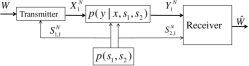
Figure 2: A channel with non-causal channel-state information at the transmitter

As shown in Figure 2, the memoryless channel with finite alphabets is characterized by $(\mathcal{X},\mathcal{Y},\mathcal{S}_{1},\mathcal{S}_{2},p_{S_{1},S_{2}},p_{Y|X,S_{1},S_{2}})$, where $X\in{\mathcal{X}}$ is the channel input; $(S_{1},S_{2})\in{(\mathcal{S}_{1},\mathcal{S}_{2})}$ is the channel-state with distribution $p_{S_{1},S_{2}}$; $p_{Y|X,S_{1},S_{2}}$ is the channel transition probability; and $(Y\in{\mathcal{Y}},S_{2}\in{\mathcal{S}_{2}})$ is the channel output, i.e., the channel-state $S_{2}$ is non-causally known at the receiver. The channel-state $S_{1}$ is non-causally known at the transmitter. In the proof of the converse, the inputs over $N$ channel uses satisfy the constraint,

$$\frac{1}{N}\sum_{n=1}^{N}\textrm{E}\left[\alpha(X_{n})\right]\leq\rho_{0},$$ (15)

where the expectation is over the information message and the state $S_{1}$.

Without input constraints, the capacity is directly obtained in [5] or can be obtained from [4] by considering $(Y\in{\mathcal{Y}},S_{2}\in{\mathcal{S}_{2}})$ as the channel output. The capacity is

$$C_{2}^{{}^{\prime}} = \max_{\mathcal{U},X=\varphi(U,S_{1}),p_{U|S_{1}}}I(U;S_{2},Y)-I(U;S_{1}),$$

where $X$ is a deterministic function of $U$ and $S_{1}$, $U\in\mathcal{U}$ is an auxiliary random variable.

With the input constraint, the capacity is

$$C_{2} = \min_{\lambda\geq 0}L_{2}(\lambda,\rho_{0})$$ (16)

$$= L_{2}(\lambda^{*},\rho_{0})$$ (17)

$$= R_{2},$$ (18)

where

$$R_{2} = \max_{\mathcal{U},X=\varphi(U,S_{1}),p_{U|S_{1}}:\textrm{E}[\alpha(X)]\leq\rho_{0}}$$ (19)

$$I(U;S_{2},Y)-I(U;S_{1});$$

$$L_{2}(\lambda,\rho_{0}) \triangleq \max_{\mathcal{U},X=\varphi(U,S_{1}),p_{U|S_{1}}}I(U;S_{2},Y)-I(U;S_{1})$$ (20)

$$\qquad\qquad-\lambda(\textrm{E}[\alpha(X)]-\rho_{0})\},$$

is the Lagrange dual function to the primary problem (19);

$$\textrm{E}[\alpha(X)] = \sum_{s_{1}}\sum_{u}p_{S_{1}}(s_{1})p_{U|S_{1}}(u|s_{1})\alpha\left(\varphi(u,s_{1})\right);$$

(18) follows from the fact that $U$ can include a time sharing variable [7] in it, and thus, $R_{2}$ is a convex $(\cap)$ function of $\rho_{0}$, and therefore, the duality gap is zero.

The traditional proof for the case with the constraint introduces a time sharing variable as follows [6].

$$I(W;Y_{1}^{N},S_{2,1}^{N})$$ (21)

$${\leq} \sum_{n=1}^{N}I(U_{n};Y_{n},S_{2,n})-I(U_{n};S_{1,n})$$

$$= N\left(I(U;Y,S_{2}|Q)-I(U;S_{1}|Q)\right)$$ (23)

$$= N(I(U,Q;Y,S_{2})-I(Q;Y,S_{2})$$

$$-I(U,Q;S_{1})+I(Q;S_{1}))$$

$$\leq N\left(I(U,Q;Y,S_{2})-I(U,Q;S_{1})\right)$$ (24)

$$= N\left(I(\bar{U};Y,S_{2})-I(\bar{U};S_{1})\right)$$ (25)

$$\leq NR_{2}$$ (26)

where $W$ is the information message; $U_{n}=(W,Y_{1}^{n-1},S_{2,1}^{n-1},S_{1,n+1}^{N})$; (21) is obtained in [5]; (23) is obtained by the definition of conditional mutual information and by letting $Q$ be uniformly distributed over $\{1,2,...,N\}$, $U=U_{Q}$, $S_{1}=S_{1,Q}$, $S_{2}=S_{2,Q}$, and $Y=Y_{Q}$; (23) follows from the chain rule of the mutual information; (24) follows from the fact that $\{S_{1,1},...,S_{1,N}\}$ are i.i.d. and thus, $I(Q;S_{1})=0$; (25) follows from defining $\bar{U}=(U,Q)$; (26) follows from $\frac{1}{N}\sum_{n=1}^{N}\textrm{E}\left[\alpha(X_{n})\right]=\textrm{E}\left[\alpha(X_{Q})\right]=\textrm{E}\left[\alpha(X)\right]\leq\rho_{0}$ and the fact that (25) is a convex $\cup$ function of $p_{X|\bar{U},S_{1}}$ when $p_{\bar{U}|S_{1}}$ is fixed, which implies that the optimal $X$ is a deterministic function of of $\bar{U}$ and $S_{1}$.

Using the Lagrangian Converse Proof, the same capacity result can be obtained without resorting to the time sharing variable:

$$I(W;Y_{1}^{N},S_{2,1}^{N})$$ (27)

$${\leq} \sum_{n=1}^{N}I(U_{n};Y_{n},S_{2,n})-I(U_{n};S_{1,n})$$

$$\leq \sum_{n=1}^{N}\cdot\left[I(U_{n};Y_{n},S_{2,n})-I(U_{n};S_{1,n})\right.$$

$$\left.-\lambda^{*}\left(\textrm{E}[\alpha(X_{n})]-\rho_{0}\right)\right],$$

$$\leq NC_{2},$$ (28)

where (27) follows from the fact that $X_{n}$’s satisfy the average power constraint.

So far, we have seen two examples where the duality gap is zero. One might worry whether the proof works when the duality gap is not zero. In the next subsection, we show that it works even when the duality gap is not zero.

II-C Capacity of Channels with Limited Feedback and Input Constraint

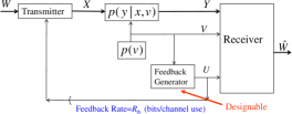
Figure 3: A channel with limited and designable feedback

We consider a channel with designable finite-rate/limited feedback. As shown in Figure 3, the memoryless channel with finite alphabets is characterized by $(\mathcal{X},\mathcal{Y},\mathcal{V},\mathcal{U},p_{V},p_{Y|X,V})$, where $X\in{\mathcal{X}}$ is the channel input, $V\in{\mathcal{V}}$ is the channel-state with distribution $p_{V}$, $p_{Y|X,V}$ is the channel transition probability, and $(Y\in{\mathcal{Y}},V\in{\mathcal{V}})$ is the channel output, i.e., the channel-state is know at the receiver. For the $n^{\textrm{th}}$ channel use, the transmitter receives a causal, but not strictly causal, finite-rate, and error free channel-state feedback $U_{n}\in{\mathcal{U}}=\{1,...,2^{R_{\textrm{fb}}}\}$ from the receiver. The feedback $U_{n}$ could be designed as a deterministic or random function of current channel-state $V_{n}$ and/or past channel-states $V_{1}^{n-1}$. Because the receiver produces $U_{n}$, it is assumed known to the receiver. In the proof of the converse, the inputs over $N$ channel uses satisfy the constraint,

$$\frac{1}{N}\sum_{n=1}^{N}\textrm{E}\left[\alpha(X_{n})\right]\leq\rho_{0},$$ (29)

where the expectation is over the information message and the feedback.

The capacity [9] of this channel without input constraint is

$$C_{3}^{{}^{\prime}} = \max_{\varphi(\cdot),p_{X|U}}I(X;Y|U=\varphi(V),V)$$ (30)

$$= \max_{\varphi(\cdot),p_{X|U}}\sum_{v}p(v)$$

$$\cdot I\left(p_{X|U}(\cdot|\varphi(v)),\>p_{Y|X,V}(\cdot|\cdot,v)\right),$$

where the important claim is that the feedback $U=\varphi(V)$ is a deterministic and memoryless function of the current channel-state $V$; in (30) the mutual information is written as a function of its input distribution and its channel transition probability.

Based on $C_{3}^{{}^{\prime}}$, one might expect the capacity with input constraint to be

$$R_{3} = \max_{\begin{array}[]{c}\varphi(\cdot),p_{X|U}:\\ \textrm{E}[\alpha(X)]\leq\rho_{0}\end{array}}I(X;Y|U=\varphi(V),V)$$ (33)

The surprising result is that the capacity may be larger than $R_{3}$.

Theorem 1

[1, 2] The capacity of the channel $(\mathcal{X},\mathcal{Y},\mathcal{V},\mathcal{U},p_{V},p_{Y|X,V})$ with designable finite-rate ($|\mathcal{U}|=2^{R_{\mbox{fb}}}$) channel-state feedback and input constraint $\rho_{0}$ is

$$C_{3} = \min_{\lambda\geq 0}L_{3}(\lambda,\rho_{0})$$ (34)

$$= L_{3}(\lambda^{*},\rho_{0})$$

$$= R_{3}+\textrm{duality gap}$$

$$\geq R_{3}$$

where

$$L_{3}(\lambda,\rho_{0}) \triangleq \max_{\varphi(\cdot),p_{X|U}}\{I(X;Y|U=\varphi(V),V)$$ (36)

$$\qquad\qquad-\lambda(\textrm{E}[\alpha(X)]-\rho_{0})\}$$

is the Lagrange dual function to the primary problem (33).

II-C1 Without the Input Constraint

We first review the key steps of the converse proof without the input constraint [2]. The mutual information between the information message and the received signal is bounded as

$$I(W;Y_{1}^{N},V_{1}^{N},U_{1}^{N})$$ (38)

$$\leq \sum_{n=1}^{N}\sum_{u_{1}^{n-1}}p(u_{1}^{n-1})$$

$$\cdot f_{3}\left(f_{1}^{(u_{1}^{n-1})}(u|v),f_{2}^{(u_{1}^{n-1})}(x|u)\right)$$

$$\leq \sum_{n=1}^{N}\sum_{u_{1}^{n-1}}p(u_{1}^{n-1})$$

$$\cdot f_{3}\left(p_{U|V}^{*}(u|v),p_{X|U}^{*}(x|u)\right)$$

$$= NC_{3}^{{}^{\prime}},$$ (39)

where (38) is obtained in [1, 2] and

$$f_{3}\left(f_{1}(u|v),f_{2}(x|u)\right)$$

$$\triangleq \sum_{v}p_{V}(v)\sum_{u}f_{1}(u|v)$$

$$\cdot I\left(f_{2}(\cdot|u),p_{Y|X,V}(\cdot|\cdot,v)\right),$$

$$f_{1}^{(u_{1}^{n-1})}(u|v) = p_{U_{n}|V_{n},U_{1}^{n-1}}(u|v,u_{1}^{n-1}),$$

$$f_{2}^{(u_{1}^{n-1})}(x|u) = p_{X_{n}|U_{n},U_{1}^{n-1}}(x|u,u_{1}^{n-1}).$$

Let $p_{U|V}^{*}(u|v)$ and $p_{X|U}^{*}(x|u)$ be the solution to

$$\max_{p_{U|V}(u|v),p_{X|U}(x|u)}f_{3}\left(p_{U|V}(u|v),p_{X|U}(x|u)\right)$$

$$= \sum_{v}p_{V}(v)\sum_{u}p_{U|V}^{*}(u|v)$$

$$\cdot I\left(p_{X|U}^{*}(\cdot|u),p_{Y|X,V}(\cdot|\cdot,v)\right).$$

Note that $p_{U|V}^{*}(u|v)$ and $p_{X|U}^{*}(x|u)$ are not functions of $u_{1}^{n-1}$ because $f_{3}(\cdot,\cdot)$ is not a function of $u_{1}^{n-1}$. Furthermore, $f_{3}\left(p_{U|V}(u|v),p_{X|U}(x|u)\right)$ is a linear function of simplex $\{p_{U|V}(u|v),u\in\mathcal{U}\}$, and thus, the optimal $p_{U|V}^{*}(u|v)$ is obtained at the extreme point $p_{U|V}^{*}(u|v)=\delta[u-\varphi^{*}(v)]$ for some deterministic function $\varphi^{*}(\cdot)$, where $\delta[x]=\begin{cases}1&x=0\\ 0&\textrm{elsewhere}\end{cases}$. Therefore, (38) and (39) are obtained.

II-C2 With the Input Constraint

The traditional method reviewed in Section II-A will not work here. One cannot produce a better feedback function and input distribution $\left(p_{U|V}(u|v),p_{X|U}(x|u)\right)$ by averaging $\left(f_{1}^{(u_{1}^{n-1})}(u|v),f_{2}^{(u_{1}^{n-1})}(x|u)\right)$ because $f_{3}\left(p_{U|V}(u|v),p_{X|U}(x|u)\right)$ is not a convex function of $\left(p_{U|V}(u|v),p_{X|U}(x|u)\right)$. However, one could introduce a time sharing variable, as shown in Section II-B, but the time sharing variable cannot be absorbed into an existing auxiliary variable of the capacity formula as in (25).

Therefore, we resort to the Lagrangian Converse Proof [2]. The key steps are

$$I(W;Y_{1}^{N},V_{1}^{N},U_{1}^{N})$$ (41)

$$\leq \sum_{n=1}^{N}\sum_{u_{1}^{n-1}}p(u_{1}^{n-1})$$

$$\cdot f_{3}\left(f_{1}^{(u_{1}^{n-1})}(u|v),f_{2}^{(u_{1}^{n-1})}(x|u)\right)$$

$$-\lambda^{*}\sum_{n=1}^{N}\left(\textrm{E}\left[\alpha(X_{n})\right]-\rho_{0}\right)$$

$$\leq \sum_{n=1}^{N}\sum_{u_{1}^{n-1}}p(u_{1}^{n-1})$$

$$\cdot f_{4}\left(p_{U|V}^{*}(u|v),p_{X|U}^{*}(x|u),\lambda^{*}\right)$$

$$= NC_{3},$$ (42)

where $\lambda^{*}$ is the solution to (1); (41) follows from the fact that the constraint is satisfied and thus $-\lambda^{*}\sum_{n=1}^{N}\left(\textrm{E}\left[\alpha(X_{n})\right]-\rho_{0}\right)\geq 0$; and

$$f_{4}\left(f_{1}(u|v),f_{2}(x|u),\lambda\right)$$

$$\triangleq \sum_{v}p_{V}(v)\sum_{u}f_{1}(u|v)$$

$$\cdot\left[I\left(f_{2}(\cdot|u),p_{Y|X,V}(\cdot|\cdot,v)\right)\right.$$

$$\left.-\lambda\left(\sum_{x}f_{2}(x|u)\alpha(x)-\rho_{0}\right)\right].$$

Let $p_{U|V}^{*}(u|v)$ and $p_{X|U}^{*}(x|u)$ be the solution to

$$\max_{p_{U|V}(u|v),p_{X|U}(x|u)}f_{4}\left(p_{U|V}(u|v),p_{X|U}(x|u),\lambda^{*}\right).$$

Again, because $f_{4}(\cdot,\cdot,\cdot)$ is not a function of $u_{1}^{n-1}$ and $f_{4}\left(p_{U|V}(u|v),p_{X|U}(x|u),\lambda^{*}\right)$ is a linear function of the simplex $\{p_{U|V}(u|v),u\in\mathcal{U}\}$, one obtains that $p_{U|V}^{*}(u|v)=\delta[u-\varphi^{*}(v)]$ and $p_{X|U}^{*}(x|u)$ are not functions of $u_{1}^{n-1}$. Therefore, (41) and (42) are obtained.

II-C3 Relation of the Lagrange Dual Function to the Time Sharing and the Capacity Region

In the following, we illustrates the central role of the Lagrange dual function $L_{3}$ from two aspects.

Time Sharing

We first discuss a time sharing expression $C_{3}^{\textrm{TS}}$ of the capacity and then show that $C_{3}^{\textrm{TS}}=C_{3}$ using the Lagrange dual function $L_{3}$. The alternative converse proof using time sharing is as follows. Define the random variable $Q_{1}$ to be uniformly distributed over $\{1,...,N\}$ and another one to be $Q_{2}=U_{1}^{Q_{1}-1}$. Then define the time sharing random variable $Q\triangleq(Q_{1},Q_{2})\in\mathcal{Q}$. We obtain

$$I(W;Y_{1}^{N},V_{1}^{N},U_{1}^{N})$$ (43)

$$\leq \sum_{n=1}^{N}\sum_{u_{1}^{n-1}}p(u_{1}^{n-1})$$

$$\cdot f_{3}\left(f_{1}^{(u_{1}^{n-1})}(u|v),f_{2}^{(u_{1}^{n-1})}(x|u)\right)$$

$$= N\sum_{q}p_{Q}(q)\sum_{v}p(v)\sum_{u}p_{U|V,Q}(u|v,q)$$

$$\cdot I\left(p_{X|U,Q}(\cdot|u,q),p_{Y|X,V}(\cdot|\cdot,v)\right)$$

$$= NI(X;Y|U,V,Q)$$

$$\leq NC_{3}^{\textrm{TS}},$$ (44)

where

$$C_{3}^{\textrm{TS}} = \max_{\mathcal{Q},p_{Q},\varphi_{Q}(\cdot),p_{X|U,Q}:\textrm{E}[\alpha(X)]\leq\rho_{0}}$$ (45)

$$I(X;Y|U=\varphi_{Q}(V),V,Q);$$

and (44) follows from the fact that (43) is a linear function of the simplex $\{p_{U|V,Q}(u|v,q),u\in\mathcal{U}\}$ and thus the deterministic feedback $U=\varphi_{Q}(V)$ does not lose the optimality.

It turns out that the Lagrange dual function $L_{3}$ in (36) is not only the dual to the primary problem $R_{3}$ in (33), but also the dual to the optimization of $C_{3}^{\mbox{TS}}$ in (45):

$$L_{3}^{\textrm{TS}}(\lambda,\rho_{0}) \triangleq \max_{\mathcal{Q},p_{Q},\varphi_{Q}(\cdot),p_{X|U,Q}}\sum_{q\in\mathcal{Q}}p_{Q}(q)\cdot$$ (46)

$$\{I(X;Y|U=\varphi(V),V,Q=q)$$

$$-\lambda(\textrm{E}[\alpha(X)|Q=q]-\rho_{0})\}$$

$$= L_{3},$$ (47)

where (47) follows the fact that the function to be optimized in (46) is a linear function of the simplex $\{p_{Q}(q),q\in\mathcal{Q}\}$ and thus, the optimal solution is obtained at certain $q^{*}$ for which $p_{Q}(q^{*})=1$. Therefore, the one dual function for two primary problems shows that $C_{3}^{\textrm{TS}}=C_{3}$.

Capacity Regions

We show that the Lagrange dual function $L_{3}$ characterizes the boundary points of the two expressions, $\mathcal{C}_{3}^{\textrm{TS}}$ and $\mathcal{C}_{3}$, of the single user capacity region. Equation (43) shows that any achievable rate $r$ under constraint $\rho$ must belong to the following capacity region:

$$\mathcal{C}_{3}^{\textrm{TS}} = \mbox{closure}\bigcup_{\mathcal{Q},p_{Q},p_{U|V,Q},p_{X|U,Q}}$$ (48)

$$\mathcal{C}_{3,\textrm{Fixed}}^{\textrm{TS}}\left(\mathcal{Q},p_{Q},p_{U|V,Q},p_{X|U,Q}\right),$$

where

$$\mathcal{C}_{3,\textrm{Fixed}}^{\textrm{TS}}\left(\mathcal{Q},p_{Q},p_{U|V,Q},p_{X|U,Q}\right)$$ (49)

$$= \left\{(r,\rho):0\leq r\leq I(X;Y|U,V,Q),\textrm{E}[\alpha(X)]\leq\rho\right\}.$$

Note that following the leads by Gallager in the study of non-convex multiple access capacity region [10], we have included $\rho$ to make the capacity region a two dimensional set. Since a convex hull performs the time sharing for you, an equivalent capacity region is

$$\mathcal{C}_{3} = \mbox{closure convex}\bigcup_{p_{U|V},p_{X|U}}$$

$$\mathcal{C}_{3,\textrm{Fixed}}\left(p_{U|V},p_{X|U}\right)$$

$$= \mathcal{C}_{3}^{\textrm{TS}},$$

where

$$\mathcal{C}_{3,\textrm{Fixed}}\left(p_{U|V},p_{X|U}\right)$$ (51)

$$= \left\{(r,\rho):0\leq r\leq I(X;Y|U,V),\textrm{E}[\alpha(X)]\leq\rho\right\}.$$

Characterizing the boundary of $\mathcal{C}_{3}^{\textrm{TS}}$ and $\mathcal{C}_{3}$ can be reduced to solving the Lagrange dual function $L_{3}$. Let $(1,-\lambda)$ be the normal vector of a hyperplane. Finding the points of $\mathcal{C}_{3}^{\textrm{TS}}$ that touch the hyperplane needs to solve

$$B_{3}^{\textrm{TS}}(\lambda) \triangleq \max_{(r,\rho)\in\mathcal{C}_{3}^{\textrm{TS}}}(1,-\lambda)\cdot(r,\rho)$$

$$= \max_{(r,\rho)\in\mathcal{C}_{3}^{\textrm{TS}}}r-\lambda\rho,$$

which can be reduced to

$$r = I(X;Y|U,V,Q)$$

$$\rho = \textrm{E}[\alpha(X)]$$

$$B_{3}^{\textrm{TS}}(\lambda) = L_{3}^{\textrm{TS}}(\lambda,\rho_{0})+\lambda\rho_{0}$$

$$= L_{3}(\lambda,\rho_{0})+\lambda\rho_{0}.$$

The same is true for $\mathcal{C}_{3}$:

$$r = I(X;Y|U,V)$$

$$\rho = \textrm{E}[\alpha(X)]$$

$$B_{3}(\lambda) = L_{3}(\lambda,\rho_{0})+\lambda\rho_{0}.$$

Therefore, we have seen that the Lagrange dual function plays the central role to connect the boundary points of the capacity region and the capacity expressions:

$$B_{3}^{\textrm{TS}}(\lambda)-\lambda\rho_{0} = L_{3}^{\textrm{TS}}(\lambda,\rho_{0})$$

$$=B_{3}(\lambda)-\lambda\rho_{0} = L_{3}(\lambda,\rho_{0})$$

$$\geq \min_{\lambda\geq 0}L_{3}(\lambda,\rho_{0})$$

$$= C_{3}(\rho_{0})=C_{3}^{\textrm{TS}}(\rho_{0})$$

$$\geq R_{3}(\rho_{0}).$$

Remark 1

Expressing the capacity as the minimum of the Lagrange dual function also helps to calculate the capacity because one does not need to worry about the time sharing while performing the optimization. If multiple solutions, i.e., input distributions etc., achieve the same value of the Lagrange dual function, then the capacity achieving strategy is a time sharing of these solutions and the time sharing coefficients are chosen to satisfy the constraint. See [1, 2] for details.

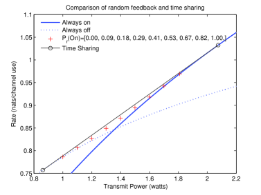
Figure 4: An example of nonzero duality gap.

Example 1

To illustrate the capacity with nonzero duality gap, we produced an example, whose detailed derivation is given in [1, 2]. The channel is an additive Gaussian noise channel with three states, good, moderate, and bad states, corresponding to small, moderate, and large noise variances. The feedback is limited to 1 bit/channel use. For small long term average power constraint, the optimal strategy is to turn on the transmitter with a fixed power only when the channel is in the good state, as shown by the dotted curve in Figure 4. For large power constraint, the optimal strategy is to turn on the transmitter when the channel is in good or moderate state with another fixed power, as shown by the solid curve in Figure 4. For the power constraint in between, the optimal strategy is a time sharing of the above two strategies, as shown by the line segment terminated by the “o”s. The gap between the line segment and the maximum of the dotted and the solid curves is exactly the nonzero duality gap between $C_{3}$ and $R_{3}$. The slope of the line segment is $\lambda^{*}$. The “+” markers are for random feedback discussed in [1, 2].

III The Extension to the Rate Distortion Theory

III-A The Converse Proof

It is straight forward to extend the Lagrangian Converse Proof to the rate distortion theory. We illustrate it using the classic i.i.d. source as an example. The rate distortion function of quantizing i.i.d. source $X$ to $\hat{X}$ in a vector manner is

$$R^{\prime}_{1}(D) = \min_{p_{\hat{X}|X}:\mbox{E}[d(X,\hat{X})]\leq D}I(X;\hat{X}),$$

where $d(\cdot,\cdot)$ measures the distortion. Use the Lagrange dual function, we have another expression

$$R_{1}(D) = \max_{\lambda\geq 0}L_{1}(\lambda,D),$$ (52)

where

$$L_{1}(\lambda,D) \triangleq \min_{p_{\hat{X}|X}}I(X;\hat{X})+\lambda\left(\mbox{E}[d(X,\hat{X})]-D\right).$$

In general, the Lagrange dual function is a lower bound and we have $R_{1}(D)\leq R^{\prime}_{1}(D)$. Due to the convexity of the mutual information, we have $R_{1}(D)=R^{\prime}_{1}(D)$.

The last few steps of the conventional converse proof is [11]

$$\sum_{n=1}^{N}I(X_{n};\hat{X}_{n})$$

$$\geq \sum_{n=1}^{N}R^{\prime}_{1}(\mbox{E}[d(X_{n},\hat{X}_{n})])$$

$$\geq nR^{\prime}_{1}\left(\frac{1}{n}\sum_{n=1}^{N}\mbox{E}[d(X_{n},\hat{X}_{n})]\right)$$

$$= nR^{\prime}_{1}(D),$$

where (III-A) used the property that $R^{\prime}_{1}(D)$ is a convex $\cup$ function of $D$.

The Lagrangian Converse Proof does not need to prove the the convexity property of $R^{\prime}_{1}(D)$ before performing the converse proof:

$$\sum_{n=1}^{N}I(X_{n};\hat{X}_{n})$$ (54)

$$\geq \sum_{n=1}^{N}\left(I(X_{n};\hat{X}_{n})+\lambda^{*}\left(\mbox{E}[d(X_{n},\hat{X}_{n})]-D\right)\right)$$

$$\geq nR_{1}(D),$$ (55)

where $\lambda^{*}\geq 0$ is the solution to (52); (54) follows from the fact that the distortion requirement is satisfied by $\hat{X}_{n}$’s and thus $\lambda^{*}\left(\left(\sum_{n=1}^{N}\mbox{E}[d(X_{n},\hat{X}_{n})]\right)-ND\right)\leq 0$; (55) follows from the fact that $R_{1}(D)$ lower bound the summand in (54) for every $n$.

The benefit of the Lagrangian Converse Proof may not appear to be significant in this simple example. But it can be easily applied to more complex cases when the time sharing has to be used in $R^{\prime}_{1}(D)$. Another example is when there are other constraints in addition to the distortion, in which case, simply introducing more Lagrange multipliers solves the problem.

III-B Dual Relation between Channel Capacity and Rate Distortion

$$C_{2}(\rho_{0}) = \min_{\lambda\geq 0}\max_{\mathcal{U},X=\varphi(U,S_{1}),p_{U|S_{1}}}I(U;S_{2},Y)-I(U;S_{1})-\lambda(\textrm{E}[\alpha(X)]-\rho_{0})$$ (56)

$$R_{2}(D) = \max_{\lambda\geq 0}\min_{\mathcal{U},\hat{X}=f(U,S_{2}),p_{U|X,S_{1}}}I(U;S_{1},X)-I(U;S_{2})+\lambda(\textrm{E}[d(X,\hat{X})]-D),$$ (57)

 

We note that using expressions involving Lagrange dual functions, the channel capacity and the rate distortion function has a pleasant symmetric form, as evident in $C_{1}(\rho_{0})$ (9) and $R_{1}(D)$ (52) for channels without side information. The symmetric form shows a dual relation in the sense of [5].

It can be easily extended to the case of non-causal side information considered in [5], where the constraints of the capacity is not considered. With the constraint, the capacity (56) and the rate distortion (57) are shown at the top of the next page. The dual relation defined in [5] is the following isomorphism.

Channel Capacity Rate Distortion

$$\min \longleftrightarrow \max$$

$$\max \longleftrightarrow \min$$

$$-\lambda \longleftrightarrow +\lambda$$

$$\textrm{Transmitted Symbol }X \longleftrightarrow \hat{X}\textrm{ Estimation}$$

$$\textrm{Received Symbol }Y \longleftrightarrow X\textrm{ Source}$$

$$\textrm{State to Encoder }S_{1} \longleftrightarrow S_{2}\textrm{ State to Decoder}$$

$$\textrm{State to Decoder }S_{2} \longleftrightarrow S_{1}\textrm{ State to Encoder}$$

$$\textrm{Auxiliary }U \longleftrightarrow U\textrm{ Auxiliary}$$

$$\textrm{Input Cost }\alpha(\cdot) \longleftrightarrow d(\cdot,\cdot)\textrm{ Distortion Measure}$$

$$\textrm{Input Constraint }\rho_{0} \longleftrightarrow D\textrm{ Distortion}.$$

A stronger dual relation is defined in [12], where the capacity and the rate distortion can be made equal by selecting proper constraints. But it does not work when the optimal solutions need time sharing. Since (56) and (57) do not include the time sharing variables, it is a future research to see whether the stronger dual relation can be established with some modification.

The dual relation for the limited feedback case is not discussed here. The reason is that the not-strictly-causal feedback to the transmitter in channel capacity corresponds to finite rate state information to the decoder in rate distortion. While the encoder in channel capacity cannot use future feedback, the decoder in rate distortion can wait to use both past and future finite rate state information.

IV Conclusions

We have introduced a simple converse proof that uses the Lagrange dual function to upper bound the information rate. It provides the following approach to deal with constraints: 1) Based on the capacity of the channel without constraints, express the capacity for the case with the constraints as the minimum of the Lagrange dual function; 2) Simply modify the converse proof for the case without the constraints by adding to the second to the last expression a term involving the Lagrange multiplier and the constraints, to produce the converse proof for the case with the constraints; 3) For the achievability, study the duality gap to determine whether the time sharing is needed.

We show that the unified capacity expression,

$$C = \min_{\lambda\geq 0}\textrm{ Lagrange Dual Function}(\lambda),$$

plays a central role to connect the characterization of the single user capacity region, the time sharing capacity formula, and the formula resulted by imposing the constraint to the maximization in the capacity formula of the case without constraints. The Lagrangian capacity formula works regardless whether the problem is convex or not. This formula also simplifies the evaluation of the capacity, by deferring the consideration of the time sharing.

The above is extended to the rate distortion theory. A symmetric form of capacity and rate distortion function is shown to demonstrate the dual relation between them. Further extension to the case of multiple constraints is straight forward. We have discussed the single letter capacity formula in this paper. The extension of the Lagrangian Converse Proof to multi-letter capacity formula, multiaccess channels, and broadcast channels is deferred to future research.

References

• [1] Y. Liu, “Capacity theorems for channels with designable feedback,” in Proc. Asilomar Conference on Signals, Systems and Computers, inivited paper, California, USA, November 2007.
• [2] ——, “Capacity theorems for single-user and multiuser channels with limited channel-state feedback,” to be submitted to IEEE Transactions on Information Theory, 2008.
• [3] S. Boyd and L. Vandenberghe, Convex Optimization.   Cambridge University Press, 2004.
• [4] S. Gelfand and M. Pinsker, “Coding for channels with random parameters,” Prob. Control and Information Theory, vol. 9, pp. 19–31, 1980.
• [5] T. Cover and M. Chiang, “Duality between channel capacity and rate distortion with two-sided state information,” IEEE Trans. Info. Theory, vol. 48, no. 6, pp. 1629–1638, 2002.
• [6] P. Moulin and J. O’Sullivan, “Information-theoretic analysis of information hiding,” IEEE Trans. Info. Theory, vol. 49, no. 3, pp. 563–593, 2003.
• [7] W. Yu and R. Lui, “Dual methods for nonconvex spectrum optimization of multicarrier systems,” IEEE Trans. Commun., vol. 54, no. 7, pp. 1310–1322, 2006.
• [8] R. G. Gallager, Information Theory and Reliable Communication.   New York, USA: John Wiley & Sons, Inc., 1968.
• [9] V. K. N. Lau, Y. Liu, and T.-A. Chen, “Capacity of memoryless channels and block fading channels with designable cardinality-constrained channel state feedback,” IEEE Trans. Info. Theory, vol. 50, no. 9, pp. 2038–2049, 2004.
• [10] R. G. Gallager, “Energy limited channels: Coding, multiaccess, and spread spectrum,” Report, LIDS-P-1714, M.I.T., Laboratory for Information and Decision Systems, November 1987.
• [11] T. M. Cover and J. A. Thomas, Elements of information theory, 2nd ed.   New York, USA: John Wiley & Sons, Inc., 1991.
• [12] S. Pradhan, J. Chou, and K. Ramchandran, “Duality between source coding and channel coding and its extension to the side information case,” IEEE Trans. Info. Theory, vol. 49, no. 5, pp. 1181–1203, 2003.