On electron-positron pair production using a two level on resonant multiphoton approximation

Abstract

We present an indepth investigation of certain aspects of the two level on resonant multiphoton approximation to pair production from vacuum in the presence of strong electromagnetic fields. Numerical computations strongly suggest that a viable experimental verification of this approach using modern optical laser technology can be achieved. It is shown that use of higher harmonic within the presently available range of laser intensities can lead to multiphoton processes offering up to 10¹² pairs per laser shot. Finally the range of applicability of this approximation is examined from the point of view of admissible values of electric field strength and energy spectrum of the created pairs.

I Introduction

Electron-positron pair production from vacuum in the presence of strong electromagnetic fields is one of the most intriguing non-linear phenomena in QED of outstanding importance specially nowadays where high intensity lasers are available for experimental verification (for a concise review see greiner , Fradkin , Grib ). The theoretical treatment of this phenomenon can be traced back to Klein Klein , SauterSauter , Heisenberg and EulerHeisenberg but it was Schwinger Schwinger that first thoroughly examined this phenomenon, often called Schwinger mechanism. Schwinger implementing the proper time method obtained the conditions under which pair production is possible: the invariant quantities $\mathcal{F=}\frac{1}{4}F_{\mu\nu}F^{\mu\nu}=-\frac{1}{2}\left(\mathcal{\vec{E}}^{2}-c^{2}\mathcal{\vec{B}}^{2}\right)$, $\mathcal{G=}\frac{1}{4}F_{\mu\nu}\tilde{F}^{\mu\nu}=c\mathcal{\vec{E}\cdot\vec{B}}$, where $F_{\mu\nu}$ and $\tilde{F}_{\mu\nu}=\frac{1}{2}\epsilon_{\mu\nu\alpha\beta}$ $F^{\alpha\beta}$ are the electromagnetic field tensor and its dual respectively, must be such that neither $\mathcal{F=}0$ , $\mathcal{G=}0$ (case of plane wave field) nor $\mathcal{F>}0$ , $\mathcal{G=}0$ (pure magnetic field). For the case of a static spacially uniform electric field (where $\mathcal{F<}0$ , $\mathcal{G=}0$) he obtained a nonperturbative result for the probability $w_{s}$ for a pair to be created per unit volume and unit time to be $w_{s}(x)\sim\sum_{l=1}^{\infty}(1/l^{2})\exp(-\frac{l\pi m^{2}}{e\mathcal{E}})$. However in order to have sizable effects the electric field strength $\mathcal{E}$  must exceed the critical value $\mathcal{E}_{c}$ $=\frac{mc^{2}}{e\lambda_{c}}\simeq 1.3\times 10^{18}V/m$ . Brezin and Itzykson Brezin  examined the case of  pair creation in the presence of a pure oscillating electric field $\mathcal{E}$ (the presence of such electric field only can be achieved by using two oppositely propagating laser beams so that in the antinodes of the standing wave formed $\mathcal{F<}0$ and pair production can occur) by applying a version of WKB approximation and treating the problem in an analogous way as in the ionization of atoms(where the three basic mechanisms multiphoton, tunneling and over the barrier ionization are present), considering the pairs as bound in vacuum with binding energy $2mc^{2}$. The probability per 4-Compton volume of $\ e^{+}e^{-}$ pair creation is given by

$$w_{BI}=\frac{e^{2}\mathcal{E}^{2}}{\pi\hbar c}\frac{1}{g(\gamma)+\frac{\gamma g^{\prime}(\gamma)}{2}}\exp\left(-\frac{\pi m^{2}}{e\mathcal{E}}g(\gamma)\right),\;\gamma=\frac{mc\omega}{e\mathcal{E}}=\frac{\hbar\omega\mathcal{E}_{c}}{mc^{2}\mathcal{E}}$$ (1)

where $g(\gamma)=\frac{4}{\pi}\int_{0}^{1}\left(\frac{1-y^{2}}{1+\gamma^{2}y^{2}}\right)^{\frac{1}{2}}dy$  and the parameter $\gamma$ $=$(Photon energy/work of$\ \mathcal{E}\$in a$\ \lambda_{Compton}$) is the equivalent of the Keldysh parameter in the ionization of atoms. The formula for $w_{BI}$ interpolates between two physically important regimes. For $\gamma\ll 1$ (high electric field strength and low frequency ), $g(\gamma)=1-(1/8)\gamma^{2}+O(\gamma^{4})$, $w_{BI}$ $\sim\exp(-\pi(\mathcal{E}_{c}/\mathcal{E})g(\gamma))$ and thus the adiabatic non-perturbative tunneling mechanism dominates. When $\mathcal{E}$ $\ll\mathcal{E}_{c}$, $w_{s}(x)\simeq w_{BI}$ . For $\gamma\gg 1$ (low electric field strength and high frequency), $g(\gamma)=(4/\pi\gamma)\ln(4\gamma/e)+O(1/\gamma^{3})$ and $w_{BI}$ $\sim(\mathcal{E}/\mathcal{E}_{c})^{2n_{0}}(1+O(1/\gamma^{2}))$ ($n_{0}=2m/\omega$). This power-law behavior of $w_{BI}$  in the external field $\mathcal{E}$, is indicative of typical multiphoton processes of order $n\geq$ $2m/\omega$ and $w_{BI}$ corresponds to the n-th order perturbation theory in $\mathcal{E}$, n being the minimum number of  photons to create a pair. Soon after the work of  Brezin and Itzykson, in the work of Popov Popov1 (see also Nikishov2 , niki ,Troup ,popov2 ) using the imaginary time method, the results of Brezin (and Schwinger ) were confirmed and investigated further by determining also the pre exponential factor in $w_{BI}$ taking in to account interference effects and treating again the system in analogous way as in the ionization of atoms. In particular, with $\tau$ being the pulse duration and $\lambda$ the electromagnetic wavelength, it was shown in Popov1 that for a spacially uniform oscillating electric field $\mathcal{E}$ with frequency $\omega$ and under the conditions $\mathcal{E}$ $\ll\mathcal{E}_{c}$, $\hbar\omega\ll$ $mc^{2}$ (which are both satisfied from present laser technology) the probabilities over a Compton 4-volume $\lambda^{3}\tau=\lambda^{4}/c$ , can be obtained for any value of $\gamma$ as a sum of probabilities $w_{n}$ of multiphoton processes of order $n$: $w_{P}=\sum_{n>n_{0}=2m/\omega}w_{n}$. For the exact rather lengthy formula of $w_{n}$, which depends on $\gamma$, $g(\gamma)$ we refer the reader to Popov1 , popov2 , Ringwald . In the case $\gamma\ll 1$ the spectrum of $n\omega$ of the $n$-photon processes is practically continuous giving the non-perturbative result $w_{P}\sim\left(\mathcal{E}/\mathcal{E}_{c}\right)^{\frac{5}{2}}\exp(-\pi(\mathcal{E}_{c}/\mathcal{E})g(\gamma))$ (see popov2 ). However in the typical multiphoton (and of perturbative nature) case $\gamma\gg 1$, $w_{n}\sim\left(\mathcal{E}/\mathcal{E}_{c}\right)^{2n}q\left(n-n_{0}\right)$ where $q\left(n-n_{0}\right)=(1/2)e^{-2\left(n-n_{0}\right)}\int_{0}^{2\left(n-n_{0}\right)}e^{t}t^{-1/2}dt$. The number of pairs created in the two regimes are given by (see popov2 )

$$N(\tau) = 2^{-3/2}n_{0}^{4}\left(\mathcal{E}/\mathcal{E}_{c}\right)^{\frac{5}{2}}\exp(-\frac{\pi\mathcal{E}_{c}}{\mathcal{E}}(1-\frac{1}{2\left(n_{0}\frac{\mathcal{E}}{\mathcal{E}_{c}}\right)^{2}}))(\omega\tau/2\pi),\;\gamma\ll 1$$ (2)

$$N(\tau) \approx 2\pi n_{0}^{3/2}\left(\frac{8\mathcal{E}_{c}}{n_{0}e\mathcal{E}}\right)^{-2n_{0}}(\omega\tau/2\pi),\;\gamma\gg 1.$$ (3)

One can easily see by comparing the above results that the multiphoton processes are by far more efficient for pair production. Treatment of Schwinger mechanism for non-oscillating electric fields and time dependent magnetic fields see also WangWong , gavgit ,cal , niki2 , kim . For the role of temporal and spacial inhomogeneities in the nonperturbative branch of pair production see kim , dunne , gies , piazza .

On the other hand the first experimental verification of $e^{-}e^{+}$ pair production took place at SLAC ( E-144 experiment)Burke where a combination of nonlinear Compton scattering and multiphoton Breit-Wheeler mechanism allowed for $e^{-}$ $e^{+}$ pair production to occur since the available electric field intensities in the area of interaction of the back-scattered photons with the laser used to produced them reached the necessary values . The number of positrons measured in 21962 laser pulses was 175$\pm 13$ and the multiphoton order of the process was found to be $n=5.1\pm 0.2(statistical)_{-0.8}^{+0.5}(systematic)$ , in very good agreement with the theory. This experiment has led to a resent interest of the subject especially as to whether modern laser technology can produce the strong electric field required for experimental verification. As explicitly analyzed by Ringwald Ringwald both for the generalized WKB or imaginary time methods, the optical laser technology available mourou , as far as power densities and electric fields concerns, does not seem to be implementable for experimental verification of $e^{-}e^{+}$ pair creation, while for the X-Ray Free Electron Laser (XFEL) should be a very promising facility (see also Melissinos , chen , tajima ).

However in a recent paper Avetissian et al Avetissian treated the problem of $e^{-}e^{+}$ production in a standing wave of oppositely directed laser beams of plane transverse linearly polarized electromagnetic waves of frequency $\omega$ and wavelength $\lambda$, using a two level multiphoton on resonant approximation. As was shown there and qualitatively argued in ctm this approach if experimentally implemented will result in much higher $e^{-}e^{+}$ production rate for the case of conventional femto-second lasers systems. The main difference of this approach to the one mentioned above is the resonance condition. Also, since the fundamental parameter of the theory is $\xi=e\mathcal{E}\mathbf{/}mc\omega\leq 1$, the results of this method can only be compared with the corresponding ones from the perturbative multiphoton regime $\gamma\geq 1$ above.

The aim of this article is to investigate further this approximation mainly focusing on numerical computations that convincingly support the possibility of experimentally detectable pair creation with available optical laser technology. Of special interest is the use of higher harmonics such as 3$\omega$ and 5$\omega$. Moreover the close resemblance of this approximation with multiphoton ionization of  atoms highlights a lot of  the physically interesting characteristics that one might expect to detect in the laboratory. In particular, ultrashort laser systems such as Nd-Yag or Ti-Sapphire, with an intensity at the fundamental frequency $\omega$, of  the order of 10${}^{22}W/m^{2}$ , when working on the multiphoton on resonant regime, is shown to produce number of pairs of the order of 10⁸ or more per laser shot. On the other hand such laser systems, with intensities up to the order of 10${}^{30}W/m^{2}$ , can provide higher harmonics pair creation, such as 3$\omega$ and 5$\omega$, where the number of pairs is shown to reach up to 10¹² per laser shot. As is demonstrated one can keep the frequency fixed and gradually change the electric field strength, and perform that for each frequency chosen. However for the laser systems under consideration it is difficult to adjust $\mathcal{E}$ while being on resonant and moreover there are limitations on the increase of it as will be shown . What is experimentally viable is to increase the frequency and, without having to focus in the diffraction limit, increase the intensity so that the resulting increase in $\mathcal{E}$ will be such that the ratio $\xi=e\mathcal{E}\mathbf{/}mc\omega$  is fixed. In section two we briefly present the results of Avetissian referring the reader to that article for their derivation. In section three we investigate the behavior of the probability density and the number of pair created by the fundamental and higher harmonics of a conventional laser with respect to changes in the electric field strength and the energy spectrum of the created electrons(positron). We end this section by showing that there exist bounds on the values of the electric field strength, the multiphoton order and the energy spectrum for the two level on resonant multiphoton approximation to hold. Finally in section four we conclude with suggested ways of experimental verification and future line of research. All numerical results have been produce for an Nd-Yag laser of photon energy $1.17eV$ and intensity 1.35$\times 10^{22}W/m^{2}$ and using Mathematica and Maple packages.

II Basic results of the two-level on resonant multiphoton approximation of pair production from vacuum.

Following Avetissian a standing wave $\overrightarrow{A}=2\overrightarrow{A}_{0}\cos\overrightarrow{k}\overrightarrow{r}\cos\omega t$ is formed by two oppositely propagating laser beams of frequency $\omega$ and wavelength $\lambda$ (see also Ringwald ). Pair production essentially occurs close to the antinodes and in spacial dimensions $l$ $\ll\lambda$ so that $\overrightarrow{k}\overrightarrow{r}=\frac{2\pi}{\lambda}l$   is very small and thus the spacial dependence of the resulting wave can be disregarded, that is $\overrightarrow{A}=2\overrightarrow{A}_{0}\cos\omega t$. Moreover since the interaction Hamiltonian is of the form $\overrightarrow{p}\overrightarrow{A}$ the most significant contribution in the pair creation process in the regions of antinodes will be at the direction along the electric field. Due to space homogeneity in these regions the 4-momentum of a particle is conserved, transitions occur between two energy levels from $\mathcal{-}E$ to $E$ by the absorption of $n$ photons and the multiphoton probabilities will have maximum values for resonant transitions

$$n=2E/\omega$$ (4)

Non-linear solutions of the Dirac equation under these conditions were obtained resulting to the following probability for an n-photon $e^{-}e^{+}$ pair creation, summed over the spin states

$$W_{n}=2f_{n}^{2}\frac{\sin^{2}\left(\Omega_{n}\tau\right)}{\Omega_{n}^{2}}$$ (5)

where

$$f_{n}=\frac{E}{4p\cos\theta}\left(1-\frac{p^{2}\cos^{2}\theta}{E^{2}}\right)^{\frac{1}{2}}n\omega J_{n}(4\xi\frac{mp\cos\theta}{E\omega})$$ (6)

$\xi$ is the relativistic invariant parameter given by,

$$\xi=\frac{e\mid\mathcal{E}_{o}\mid}{mc\omega}\lesssim 1$$ (7)

$\Omega_{n}$ and $\Delta_{n}$ is the ’Rabi frequency’ of the Dirac vacuum at the interaction with a periodic electromagnetic field and respectively given by,

$$\Omega_{n}=\sqrt{f_{n}^{2}+\frac{\Delta_{n}^{2}}{4}}\ll\omega,\;$$ (8)

$\theta$ is the angle between the momentum of $e^{-}\left(e^{+}\right)$ and $A_{0}$, $\mathcal{E}_{o}$ is the amplitude of the electric filed strength of one incident wave, $\Delta_{n}=2E-n\omega$ is the detuning of resonance, and $\tau$ is the interaction time. In obtaining the above probability it has been assumed without loss of generality that $p_{z}=0$ since there is a symmetry with respect to the direction of $A_{0}$ (taken to be the Oy axis) and thus $\mathbf{p}=(p_{x}=p\sin\theta,p_{y}=p\cos\theta,0)$. As usual in applying the resonance approximation on a two level system the probability amplitudes are slow varying functions which is equivalently expressed here by the condition in (8), corresponding to such field intensities for which the condition in (7) is satisfied. For short interaction time i.e. when $\Omega_{n}\tau\ll 1$, $\frac{\sin^{2}\left(\Omega_{n}\tau\right)}{\Omega_{n}^{2}}\rightarrow 2\pi\tau\delta\left(\Delta_{n}\right)$ and the differential probability per unit time summed over the spin states in the phase-space volume $Vd^{3}p/\left(2\pi\right)^{3}$  is $dw_{n}=\frac{1}{2\pi^{2}}f_{n}^{2}\delta(2E-n\omega)Vd^{3}p$ which after integration over the $e^{-}$($e^{+}$) energy, the angular distribution of a n-photon differential probability of the created $e^{-}$, $e^{+}$ pair, per unit time in unit space volume ($V=1$), on exact resonance is given by:

$$\frac{dw_{n}}{do}=\frac{n\omega}{8\pi^{2}}f_{n}^{2}\left(n^{2}\omega^{2}-4m^{2}\right)^{\frac{1}{2}}$$ (9)

where $do=\sin\theta d\theta d\varphi$. The total angular distribution of probability is $\frac{dw}{do}=\sum_{n=n_{0}}\frac{dw_{n}}{do}$ (where $n_{0}=2mc^{2}/\hbar\omega$ is the threshold number of photons for the pair production process to occur) and integrating over the solid angle we obtain the total probability per unit time in unit space volume of the $e^{-}$, $e^{+}$ pair production $w=\sum_{n=n_{0}}w_{n}$ as:

$$w = \sum_{n=n_{0}}\frac{n^{5}\omega^{5}}{32\pi p}((\frac{2Z_{0}^{2}}{4n^{2}-1}-1)J_{n}^{2}\left(Z_{0}\right)+\frac{Z_{0}^{2}J_{n-1}^{2}\left(Z_{0}\right)}{2n(2n-1)}+\frac{Z_{0}^{2}J_{n+1}^{2}\left(Z_{0}\right)}{2n(2n+1)}$$ (10)

$$-\frac{4p^{2}}{n^{2}\omega^{2}}\frac{Z_{0}^{2n}}{\left(2n+1\right)\left(n!\right)^{2}2^{2n}}\times\;_{2}F_{3}\left(n+\frac{1}{2},n+\frac{1}{2};n+1,2n+1,n+\frac{3}{2};-Z_{0}^{2}\right))$$

where $Z_{0}=\left(\frac{4\xi m}{\omega}\right)\left(1-\frac{4m^{2}}{n^{2}\omega^{2}}\right)^{\frac{1}{2}}$. The total number of pairs $N$ created for a given laser characteristics can be estimated by (see Avetissian )

$$N\sim wV\tau,\;V\sim\sigma^{2}l$$ (11)

where $V$ is the space-volume, $\sigma$ is the cross section radius, $l\ll\lambda$ as stated above and $\tau$ is the interaction time. For focused optical lasers in the diffraction limit $\sigma\sim\lambda$ $\sim 10^{-6}m$ and $\tau\sim 10^{-14}s$. For the investigation that will follow

$$\frac{dN_{n}}{do}=\frac{dw_{n}}{do}V\tau$$ (12)

is the angular distribution of the number of pairs created from an $n$-photon process and

$$N_{n}=w_{n}V\tau$$

is the number of pairs created from that process.

III Numerics and applicability of the on resonant multiphoton approximation of pair production from vacuum.

As can be seen from section II a basic role in the physical interpretation of the numerical computations that will follow, is played by the function $f_{n}$ (Rabi frequency on exact resonance), as the probabilities and number of produced pairs obtained are heavily depend on its behavior (see (5), (9)). For a given value of the $\xi$ and $n$, as can be seen from (6), $\ f_{n}$ and all derived angular dependent quantities in the above section, maximizes at $\ \theta=0$ and this is true for every $\xi$ and $n$. Consequentially we shall concentrate our analysis at this angle of observation of created pairs. Not only this simplifies the numerics that will be presented below but also helps to clarify the behavior of this approximation in particular as far as future experimental verification. From now on $c$ and $\hbar$ should be explicitly stated in the formulas. On exact resonance, $n$ is given by (see 4)

$$n=2E/\hbar\omega=2qmc^{2}/\hbar\omega,\;q\geq 1,$$ (13)

where we have expressed the energy $E$ of the created electron (positron) in terms of its rest energy as $E=qmc^{2}$. Thus $q$ characterizes the spectrum of the created pairs. At $\ \theta=0$, a suitable expression for $f_{n}$, $f_{n}$, can be obtained from (6) with $E=qmc^{2}$, $p=(1/c)\sqrt{E^{2}-m^{2}c^{4}}$, and using the asymptotic behavior of the Bessel function $J_{n}(x)$ at $x\simeq n$ (see also Avetissian ). In fact, as can be seen from (13) for optical lasers where $\omega$ is very small (of the order of $eV$), $n$ is very large and as $\xi\lesssim 1$, the argument of the Bessel function in (6), which now becomes $x=\frac{2n\xi}{q}\left(1-\frac{1}{q^{2}}\right)^{\frac{1}{2}}$, is also very large and of the same order as $n$, not mentioning Bessel’s extreme sensitivity on $\xi$ too. Thus to obtain executable numerical computations, we shall from now on adopt this asymptotic behavior of the Bessel function by writing $J_{n}(x)=J_{n}(nsecha)=(1/\sqrt{2\pi ntanha})\exp\left(ntanha-na\right)$ where $a$=$sech^{-1}(\frac{2\xi}{q}\left(1-\frac{1}{q^{2}}\right)^{\frac{1}{2}})$. Then $f_{n}$ is given by

$$f_{n}=\frac{1}{4}\left(q^{2}-1\right)^{-\frac{1}{2}}n\hbar\omega\frac{\exp\left(ntanha-na\right)}{\sqrt{2\pi ntanha}}$$ (14)

The function $f_{n}$ can now be used together with (9) and (12), to obtain the number of pairs at $\ \theta=0$, $N_{0}=\frac{dN_{n}}{do}|_{\theta=0}$ as

$$N_{0}=\frac{dN_{n}}{do}|_{\theta=0}=\frac{1}{4\pi^{2}}\frac{V\tau}{V_{e}}\frac{q\sqrt{q^{2}-1}}{m^{2}c^{4}}f_{n}^{2}$$ (15)

where $V_{e}=7.4\times 10^{-59}m^{3}s$ is the four Compton volume of an electron.

Using (13), (14), the envelope of $\ f_{n}$ as a function of $q$ can be plotted for fixed values of  $\xi$. This allow to investigate the envelop of  $\ f_{n}$, from electric field strength , frequency of radiation or both point of view. In fig.1(a) (see also Avetissian ),  we plot the envelops of $\ \ f_{n}$, for the case of $\omega=1.17eV$ , $3\omega$ and $5\omega$ and for values of $\xi=0.9995$, $0.9990$ and $0.9987$ respectively. The corresponding electric fields $\mathcal{E}_{o}$ are approximately given by (7) as $3.\,\allowbreak 024\,2\times 10^{12}$ V/m, $9.\,\allowbreak 068\,1\times 10^{12}V/m$, $1.\,\allowbreak 510\,9\times 10^{13}V/m$. Each point in a curve of fig.1(a) corresponds via (13) to an order $n$ multiphoton process and to an energy $E=qmc^{2}$ of the  electron (positron) to be created in the area of antinodes under the application of fixed field strength and frequency. The most probable process corresponds to the peaks of the curves which will be labeled with the triplet ($n_{p}$ ,$q_{p}$, $\xi$). For the three cases of fig.1(a) , using common differential calculus, we find peaks approximately at ($1.2369\times 10^{6}$, $1.41408$, $0.9995$), ($4.1226\times 10^{5}$, $1.41395$, $0.9990$) and ($2.4734\times 10^{5}$, $1.41387$, $0.9987$) respectively.

Figure 1: (a) The envelops of $f_{n}$(at $\theta=0$), as a function of the units of rest energy $q$, for $\xi=0.9987$ and $5\omega$ (top curve), $\xi=0.9990$ and $3\omega$ (middle curve) and $\xi=0.9995$ and $\omega=1.17eV$ (bottom curve), $k=10^{21}$. (b) The envelops of $f_{n}$(at $\theta=0$) as a function of the units of rest energy $q$ for $\xi=0.9987$ and for $\omega=1.17eV$ (bottom curve with $k=10^{40}$), $3\omega$ (middle curve with $k=10^{24}$), $5\omega$ (top curve with $k=10^{21}$).

A quite interesting case when dealing with higher harmonics is to investigate the behavior of $f_{n}$(at $\ \theta=0$) for $\xi$ fixed. As we change from $\omega$ to $2\omega$, $3\omega$ etc., an appropriate, experimentally viable, increase of the laser intensity can lead $\mathcal{E}_{o}$ to increase by the same amount as $\omega$. In fig.1(b), such case is presented for $\xi=0.9987$ and $\omega=1.17eV$ , $3\omega$ and $5\omega$ where the corresponding envelops have peaks ($n_{p}$ ,$q_{p}$) at (1.2367$\times 10^{6}$, 1.41390), (4.1223$\times 10^{5}$, 1.41388) and (2.4734$\times 10^{5}$, 1.41387) respectively. Both from fig.1(a, b), it is seen that passing to higher harmonics the peak value of $\ f_{n}$ increases rapidly leading to an increase of the probability of pairs created., with a subsequent decrease of  the most probable multiphoton order $n_{p}$ and corresponding energy $E_{p}=$ $q_{p}mc^{2}$ of electron(positron) created. Moreover the range of the energy spectrum of the pairs broadens thus facilitating their observation: from approximately $0.720MeV$ to $0.726MeV$ which is for $\omega$ , to, $0.715MeV$ to $0.731MeV$ which is for 5$\omega$. An explanation for the choices of values for $\xi$ will be conferred till the end of this section.

Corresponding to each envelop of $\ f_{n}$ we can plot the envelop of  the number of pairs created by n-photon processes $N_{0}$ , as a function of  $q$, using (9), (12), (13), (14), (15). Examples are presented in fig.2(a) (see also fig.1(a)) for the cases $\omega=1.17eV$ , $3\omega$, $5\omega$ and for values of $\xi=0.9995$, $0.9990$ and $0.9987$ respectively. The four volume used in each case has been calculated by (11), with $\tau\sim 10^{-14}s$ , $\lambda=1.074\times 10^{-6}$m and $\sigma\sim 10^{-5}m$, leading to $V\tau\sim\sigma^{2}l\tau\sim\sigma^{2}(0.1\lambda/k)\tau,$ where $k=1,3,5$ for the corresponding harmonics. Note that we do not necessarily have to work in the diffraction limit $\sigma\sim\lambda$ as the number of pairs created is adequately high for observation, while to conform with the developed approximation where $l\ll\lambda,$ the choice $l=0.1\lambda/k$ demonstrates the fact that when going to higher harmonics the area close to the antinodes that the pair creation essentially happens decreases. Each of these curves essentially give the energy spectrum of the created number of pairs at $\theta=0$ after the application of a fixed electric field strength and laser frequency and for all $n$-photon process at exact resonance. Their peaks can be labeled by the triplet ($N_{p}$ ,$q_{p}$, $\xi$), $N_{p}$ being the maximum (and most probable) number of pairs created for the $n_{p}$-photon processes of fig.1(a). These three cases have peaks approximately at (5.856$\times 10^{8}$,1.41408, $0.9995$), (1.815$\times 10^{9}$,1.41395, $0.9990$) and ( 2.372 $\times 10^{10}$,1.41387, $0.9987$) respectively. The corresponding values of  $\mathcal{E}_{o}$ and the range of the energy spectrum are as those in fig.1(a) above. Experimentally such curves are important as one can detect the electron(positron) energies coming up from the various $n$-photon processes for a given $\mathcal{E}_{o}$ and laser frequency and compare with these theoretical estimates.

Figure 2: (a) Envelop of number of pairs created $N_{0}$, as a function of the units of rest mass $q$, at angle $\theta=0$ for the multiphoton processes $\omega=1.17eV$ (bottom curve with $k=10^{-7}$), $3\omega$ (middle curve with $k=10^{-7}$) and $5\omega$ (top curve with $k=10^{-8}$) of fig.1(a).(b)Envelop of number of pairs created $N_{0}$, as a function of the units of rest mass $q$, at angle $\theta=0$ and $\xi=0.9987$, for the multiphoton processes $\omega=1.17eV$ (bottom curve with $k=10^{29}$), $3\omega$ (middle curve with $k=10^{-2}$) and $5\omega$ (top curve with $k=10^{-8}$) of fig.1(b).

The case corresponding to fig.1(b) is presented in fig.2(b), where for $\omega=1.17eV$ , $3\omega$ and $5\omega$ and  $\xi=0.9987$ fixed (and thus for $\mathcal{E}_{0}$, 3$\mathcal{E}_{0}$ and $5\mathcal{E}_{0}$), the corresponding envelops have peaks ($N_{p}$ ,$q_{p}$) approximately at (2.430$\times 10^{-28}$, 1.41390), (1.104$\times 10^{4}$, 1.41388) and ( 2.391 $\times 10^{10}$, 1.41387)  corresponding to the $n_{p}$-photon processes of fig.1(b). It is easily seen from both these figures that going to higher harmonics, the number of pairs increases very rapidly with simultaneous increase of the range of energies of the pairs but decrease of their maximum energy.

We turn now to a commonly experimentally verifiable behavior of multiphoton processes given by the log-log plot of the number of particles created versus the value of electric field strength $\mathcal{E}_{o}$. In fig.3 we present the log-plots of the number of pairs $N_{0}$ as a function of $\xi$ , using (9), (12), (13), (14), (15), for three on resonant multiphoton process with $n_{1}\sim 1.\,\allowbreak 233\times 10^{6}$ ($q\sim 1.41$), $n_{2}\sim 1.237\times 10^{6}$ ($q\sim 1.4141$) and $n_{3}\sim 1.\,\allowbreak 242\times 10^{6}$ ($q\sim 1.42$) chosen from the bottom curve of fig.1(a) where $\omega=1.17eV$ is kept fixed (see also bottom curve of fig.2(a)). Note that the energies of the created particles for each of the above on resonance multiphoton processes are close enough given approximately by $E_{1}$ $\sim$0 .721 MeV, $E_{2}$ $\sim$ $0.723\,$MeV and $E_{3}$ $\sim\allowbreak 0.726$ MeV respectively while the range of change of $\mathcal{E}_{o}$ producing observationally enough pairs is between $3.\,\allowbreak 023\,8\times 10^{12}$ V/m to $3.\,\allowbreak 024\,5\times 10^{12}$V/m. The range of change of $\mathcal{E}_{o}$ (and thus of $\xi)$ is very small even for higher harmonics because of the extreme sensitivity of the Bessel function and its approximation in $\xi$. This suggests that an experimental verification of such curves is rather difficult for optical lasers. As $\omega$ is fixed and thus the appearance of the different on resonant multiphoton processes originate only from the different energies involved (see values of $q$), crossings in these curves, which traditionally appear in multiphoton ionization, are not to be expected. Further more, as will be explained in the end of this section, such curves terminate from above for a maximum value of $\mathcal{E}_{o}$ (and thus of $\xi)$ .

Figure 3: Log-plot of the number of pairs created $N_{0}$, as a function of $\xi$, at angle $\theta=0$, for three multiphoton processes from the bottom curve of fig.1, with $q=1.41$ (middle curve) , $q\sim\sqrt{2}$ (top curve) and $q=1.42$ (bottom curve).

In fig.4(a) we give the log-plot of the number of pairs $N_{0}$ versus $\xi$ for the most probable multiphoton processes of $\omega=1.17eV$ , $3\omega$, $5\omega$ of fig.1(a) (see also fig.2(a)) where ($n_{p}$ ,$q_{p}$, $\xi$)$\sim$($1.2369\times 10^{6}$, $1.41408$, $0.9995$), ($4.1226$ $\times 10^{5}$, $1.41395$, $0.9990$) and ($2.4734$$\times 10^{5}$, $1.41387$, $0.9987$) respectively . In contrast with the case presented in fig.3, crossings are expected as the laser frequency changes. However for the developed approximation, the values of $\xi$ where these occur are not applicable as $\xi$ $>1$. Similar results arise when we consider the most probable multiphoton processes ($n_{p}$ ,$q_{p}$, $0.9987$) of fig.1(b) (see also fig.2(b)) and are presented in fig.4(b), where for $\omega$, 3$\omega$ and 5$\omega,$ ($n_{p}$ ,$q_{p}$)$\sim$(1.2367$\times 10^{6}$, 1.41390), (4.1223$\times 10^{5}$, 1.41388) and (2.4734$\times 10^{5}$, 1.41387) respectively.

Figure 4: (a) Log-plot of the number of pairs created $N_{0}$, as a function of $\xi$, for the most probable multiphoton processes of fig.1(a) with $\omega=1.17eV$ (bottom curve) , $3\omega$ (middle curve) and $5\omega$ (top curve). (b) Log-plot of the number of pairs created $N_{0}$, as a function of $\xi$, for the most probable multiphoton processes of fig.1(b) with $\omega=1.17eV$ (bottom curve) , $3\omega$ (middle curve) and $5\omega$ (top curve).

Given an initial laser frequency and power density, the obvious question to be raised concerns on one hand the range of possible multiphoton processes that can be obtain within this approximation (or equivalently the range of energy of the created pairs per rest energy of e^- , $q$ ) and on the other hand the range of values of $\xi$ (or equivalently of the electric field strength $\mathcal{E}_{0}$) for which these are realized. The physical acceptable values of $\xi$, $q$ have not only to conform with the condition of applicability of resonant approximation $\Omega_{n}\ll\omega$ (i.e.$\xi\precsim 1$) but also to energy considerations stating that the energy per laser shot, $E_{b}$ , provided by the incident beam , should not be less than the total energy of the pairs created, that is

$$E_{b}\geqslant 2qmc^{2}N$$ (16)

where $N$ is the total number of pairs created. $E_{b}$ can be calculated from the available power density of the laser $S_{b}=\frac{1}{\mu_{0}c}$ $\mathcal{E}_{0}^{2}$ as

$$E_{b}=S_{b}\pi\sigma^{2}\tau$$ (17)

where $\sigma$ is the radius of the cross section and $\tau$ is the pulse duration. To get a sufficiently convincing answer to the above question we can consider the energy difference

$$\Delta E_{b}=S_{b}\pi\sigma^{2}\tau-2qmc^{2}N_{0}$$ (18)

which by means of (14) and (15) is considered as a function of $\xi$(or $\mathcal{E}_{0}$) and $q$(or $n$) . Keeping $E_{b}$ fixed (i.e. for given laser characteristics $\omega$, $S_{b}$, $\sigma$, $\tau$) and for a given $q\geq 1$, $\xi$ can be increased up to a value $\xi=h$ (or maximum $\mathcal{E}_{0}$) for which $\Delta E_{b}=0$(minimum physically acceptable value of $\Delta E_{b}$) provided that $h\ngtr 1$. Consequentially, for given values of $q,$ we can quit sufficiently estimate the applicability of the present approximation by numerically computing the upper bounds $h$ of $\xi$, using $S_{b}\pi\sigma^{2}\tau=2qmc^{2}N_{0}$ (of course we could also keep $\xi\precsim 1$ fixed and numerically compute $q$, but for experimental reasons, we are merely interested in the maximum applicable $\mathcal{E}_{0}$ for the present approximation to hold). In fig.5

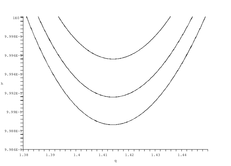
Figure 5: Upper bound $h$ of $\xi$ as a function of $q$ for the cases $\omega=1.17eV$ (top curve), $3\omega$ (middle curve) and $5\omega$ (bottom curve).

we plot the maximum admissible values $h$ of $\xi$ (or $\mathcal{E}_{0}$) as a function of $q$ (and thus of $n$), for the three cases $\omega$, 3$\omega$ and 5$\omega$ where computations have been performed using $\Delta E_{b}=0$ for $\omega=1.17eV$, $S_{b}=s\times 1.35\times 10^{22}W/m^{2}$ ($s=1,3^{2},5^{2}$ respectively), $\sigma\sim 10^{-5}m$ and $\tau\sim 10^{-14}s$. The factor $s$ in $S_{b}$ is justified by the approach adopted to increase the laser intensity in order to increase $E_{b}$ , rather than going to the diffraction limit ($\sigma\sim\lambda^{\prime}$) to increase it, as this would be experimentally tedious when going to higher harmonics $\omega^{\prime}=k\omega$, where $\lambda^{\prime}=\lambda/k,$ $k=1,2,3...$. From the curves of fig.5 the range of the applicable on resonant multiphoton processes can easily be read off via the range of values of $q$ shown and using (13). Moreover the maximum applicable values of $\xi$ (and thus via (7) of $\mathcal{E}_{0}$) for each one of them can also be read off. Points ($q$, $h$) for $h>1$ are unacceptable for the two level on resonant approximation of pair production. Also because of the existence of $h$ for each $q$ (and $n$) points in the log-plots of figs 3,4(a, b), where $\xi>h$ should be disregarded, and thus the curves for these plots should be terminated at $\xi=h$ or equivalently at $\mathcal{E}_{0}=\mathcal{E}_{0\max}=hmc\omega^{\prime}/e$. That is also why crossing points cannot be present in the log-plots.

As an example of the above consider the three peak points of the curves $\omega$, $3\omega$, $5\omega$ in fig.2(a). The $q_{p}$ values of these points are situated close to the bottom of the corresponding curves of fig. 5 from which we can infer their corresponding $h$s to be approximately $h\sim 0.99956$, $0.99916$, $0.99886$. Moreover as can be seen from fig. 4(a, b), when $\xi$ approaches $h$ the number of pairs created for the corresponding $n_{p}$ multiphoton processes reaches a maximum value. This explains the choices of $\xi$ chosen in the above numerical computations to be close to $h$. Consequentially points ($\xi$, $N_{0}$) in figs 3, 4(a, b) with values of $\xi>h$ should not be taken in to account.

Another important consequence of the upper bound $h$, concerns the value of $\xi$ chosen when examining the spectrum of created pairs, for fixed $\omega^{\prime}$, via plots of fig.2(a, b). For simplicity consider $\omega^{\prime}=\omega$. In fig.3 the three terminal points of these curves, which maximize $N_{0}$, corresponds to the points (1.41, 0.99957), ($\sqrt{2}$, 0.99956), (1.42, 0.99959) of the $\omega$-curve of fig.5, ($\sqrt{2}$, 0.99956) being the lowest point of it. If one chooses to work with an $h\neq$0.99956, say $h=$0.99959, then fig.3 shows that energies with $q<1.42$ can never be observed. However plots such as fig.2(a) with $\xi=$0.99959 can be drawn showing that points with values of $q$ in the physically forbidden range do contribute in $N_{0}$. Obviously this is a completely unphysical situation and should be taken care in experimental verification of plots such as fig.2(a, b). In fact the only consistent value of $\xi$ is the one of the lowest point ($q_{l\text{ }}$, $\xi=h_{l}$) of the $\omega^{\prime}$-curve of fig.5 as this guarantees both observability of all energies around $q_{l\text{ }}=q_{p\text{ }}$ as given in fig.2(a, b) and maximization of $N_{0}$ for this $q_{p}$.

IV Conclusion

From the above analysis it is evident that present ultrashort laser technology seems to suffices in order to experimentally verify the validity of $e^{+}e^{-}$ pair production from vacuum using a two level on resonance multiphoton approximation. In particular, emphasis has been given in the implementation of higher harmonics such as 3$\omega$ and 5$\omega$ while the electric field strengths required, are obtained by increasing the laser energy rather than focusing to the diffraction limit. This improves the model in various advantageous ways. The need of higher harmonics is dictated by the limitation imposed by the upper value of electric field $\mathcal{E}_{o}$ of the fundamental due to the condition $\xi=\frac{e\mathcal{E}_{o}}{mc\omega}\lesssim 1$. In order to work with $\xi\lesssim 1$ but increase the $\mathcal{E}_{o}$ higher $\omega$ values are necessarily.

Firstly, as shown in figs 1, 2, the range of the created spectrum widens and the maximum number of pairs created increases drastically reaching $N_{0}=$10¹² pairs per laser shot for 5$\omega$ while, because of the resonant condition, the electric fields needed are low $\mathcal{E}_{0}$ $\sim 10^{13}V/m$, compared with other multiphoton approximations such as the one leading to (3). In fact this is mainly why there is no need to focus in the diffraction limit to achieve such electric fields as present laser energies and achievable power can provide them.

Secondly the confirmation of the power law behavior of the number of pairs created as a function of electric field strength, typical of multiphoton processes, is demonstrated by figs 3, 4, showing again a drastic increase of $N_{0}$ in higher harmonics. However such log-plots can not probably be subjected to experimental verification since the range of  change of  $\mathcal{E}_{0}$ is very small and thus difficult if not technically impossible to be performed. However what it is suggested in the present work is the verification of higher harmonic curves of fig.2, of the number of pairs $N_{0}$versus their spectrum, when measuring the number and the momenta of the created electrons(positrons) at angle $\theta=0$.

Finally the range of applicability of this approximation have been investigated and the results are presented in fig.5. In particular working with a chosen frequency, for each q there exists a maximum value $\xi=h$ and thus a maximum electric field $\mathcal{E}_{0\max}$ that can be used. As has been demonstrated by the analysis of fig.5 in section III there important consequences for a potential experimental verification of the suggested plots of fig.2(a, b). Consequently one can describe the following attractive experimental scenario. Initially one should choose a laser energy $E_{b}$ capable of generating a higher harmonic $\omega^{\prime}=k\omega$ beam. Then by appropriate focusing, increase the electric field at the value $\mathcal{E}_{0\max}=h_{l}mck\omega/e$ where $h_{l}$ is the lowest value of the $k\omega$ curve of fig.5, and form the standing wave as required by the theory. The number of pairs $N_{0}$ created at the antinodes versus their spectrum will be given by figures such as those of fig.2(a, b) drawn for $\xi=h_{l}$. Then $N_{0}$ maximizes for pairs with energy $E=2q_{p}mc^{2}$ where ($q_{p}$, $h_{l}$) is the lowest point of the $k\omega$ curve of fig.5. Higher harmonics thus give a wider pair spectrum and a lower $\mathcal{E}_{0\max}$ value required, both been of great experimental advantage.

In concluding one should state that use of XFEL technology (equivalent to ultrahigh harmonics) overcomes the difficulties of so high order of multiphoton processes present in the optical regime, while giving a wider range of electric field changes. Investigations along the lines of the present article of the application of the resonant approximation using XFEL are in progress.

References

- (1) W. Greiner, B. Muller, J. Rafelski, ‘Quantum Electrodynamics of Strong Fields’, Springer – Verlag, Berlin, 1985.
- (2) E. S. Fradkin, D. M. Gitman and Sh. M. Shvartsman, ’Quantum Electrodynamics with unstable vacuum’ Springer-Verlag, Berlin, 1991.
- (3) A. A. Grib, S. G. Mamaev and V. M. Mostapanenko, ’Vacuum Quantum Effects in Strong Fields’ Atomizdat, Moscow, 1998; Fr iedmann Laboratory Publishing, St. Petersburg 1994.
- (4) O. Klein, Z. Phys., 53, 157 (1929).
- (5) F. Sauter, Z. Phys. 69, 742 (1931).
- (6) W. Heisenberg, H. Euler, Z. Phys. 98, 718 (1936).
- (7) J. W. Schwinger, Phys. Rev., 82, 664 (1951).
- (8) E. Brezin and C. Itzykson, Phys. Rev. D 2, 1191 (1970).
- (9) V.S. Popov, JETP Lett. 13, 185 (1971); Sov. Phys. JETP 34, 709 (1972); Sov. Phys. JETP 35, 659 (1972); V.S. Popov and M. S. Marinov, Sov. J. Nucl. Phys.16, 449 (1973) ; JETP Lett. 18, 255 (1974); Sov. J. Nucl. Phys., 19, 584 (1974).
- (10) A. I. Nikishov, Nucl. Phys. B21, 346 (1970).
- (11) N.B. Narozhnyi and A. I. Nikishov, Sov. J. Nucl. Phys.11, 596 (1970); Sov. Phys. JETP, 38, 427 (1974).
- (12) G.J. Troup and H.S. Perlman, Phys. Rev. D 6, 2299 (1972).
- (13) V.S. Popov, Phys. Let. A298, 83 (2002).
- (14) A. Ringwald, Phys. Let. B 510, 107 (2001).
- (15) R.C. Wang and C.Y. Wong, Phys. Rev. D 38, 348 (1988).
- (16) S. P. Gavrilov and D. M. Gitman Phys. Rev. D 53, 7162 (1995).
- (17) G. Calucci, ”Pair production in a time dependent magnetic field”, hep-th/9905013.
- (18) A. I. Nikishov, ”On the theory of scalar pair production by a potential barrier”, hep-th/0111137.
- (19) S. P. Kim and Don N. Page, Phys. Rev. D73 : 065020, (2006); ”Schwinger pair production in electric and magnetic fields” hep-th/0301132.
- (20) G. V. Dunne, Q. Wang, H. Gies and C. Schubert, Phys. Rev. D73 : 065028, (2006); hep-th/0602176.
- (21) H. Gies and K. Klingmuller, Phys. Rev. D72 : 065001, (2005); hep-ph/0505099.
- (22) A. DiPiazza, Phys. Rev. D70 : 053013, (2004);
- (23) D.L. Burke et. al., Phys. Rev. Let., 79, 1626 (1997).
- (24) M. Perry and G. Mourou, Science 264, 917 (1994).
- (25) A.C. Melissinos, in Quantum Aspects of Beam Physics, Proc.15th Advanced ICFA Beam Dynamics Workshop, Monterey, Cal., 4-9 Jan 1998 (World Scientific, Singapore, 1998) p. 564.
- (26) P. Chen and C. Pellegrini, in Quantum Aspects of Beam Physics, Proc.15th Advanced ICFA Beam Dynamics Workshop, Monterey, Cal., 4-9 Jan 1998 (World Scientific, Singapore, 1998) p. 571.
- (27) P. Chen and T. Tajima, Phys. Rev. Lett. 83, 256 (1999).
- (28) H. K. Avetissian, A. K. Avetissian, G. F. Mkrtchian and Kh. V. Sedrakian, Phys. Rev. E 66, 016502 (2002).
- (29) C. Kaberidis, I. Tsohantjis and S. Moustaizis ’Multiphoton approach on pair production under the light of recent experimental and theoretical investigations’, Proceedings of the Sixth International Symposium ‘Frontiers of Foundamental and Computational Physics’ Udine, Italy, 26-29 September 2004, Sidharth B.G, Honsell F., de Angelis A. (Eds.) 2005 pp. 279-283