Ultrafast manipulation of electron spins in a double quantum dot device: A real-time view

Abstract

We consider a double quantum dot system with two embedded and non-aligned spin impurities to manipulate the magnitude and polarization of the electron spin density. The device is attached to semi-infinite one-dimensional leads which are treated exactly. We provide a real-time description of the electron spin dynamics when a sequence of ultrafast voltage pulses acts on the device. The numerical simulations are carried out using a spin generalized and modified version of a recently proposed algorithm for the time propagation of open systems [Phys. Rev. B 72, 035308 (2005)]. Time-dependent spin accumulations and spin currents are calculated during the entire operating regime which includes spin injection and read-out processes. The full knowledge of the electron dynamics allows us to engineer the transient responses and improve the device performance. An approximate rate equation for the electron spin is also derived and used to discuss the numerical results.

I Introduction

The ability of controlling magnitude and orientation of electron spin densities in integrated molecules and quantum dots is of utmost importance to bring quantum computation closer to real life.nc.2000 ; asl.2002 The microscopic description of nanoscale spin devices like, e.g., the two-quantum-bit gate envisaged by Loss and Di Vincenzo,ldv.1998 constitutes a challenging problem in the theory of open systems far from a steady state. Research activities in the emerging field of spin-dependent transportms.2002 have mainly focussed on steady-state properties. Only very recently the transient dynamics of spin polarized currents through quantum dots has attracted some attention,mba.2005 ; fhs.2006 ; slgj.2007 ; s.2007 partly due to experimental advances in manipulating electronic densities with ultrafast voltage pulses.hfcjh.2003 ; hwvwbek.2003 ; ehvbwvk.2004 ; hvbvenkkv.2005 ; pjtlylmhg.2005 ; kbtvnmkv.2006 ; kstbfajfrp.2007 This paper goes in the same direction and wants to be a further step toward the bridging of spin dependent transport and fundamental quantum computation. We perform time-dependent simulations of the charge and spin dynamics of a nanoscale device in contact with one-dimensional leads. The semi-infinite leads are treated exactly. The results are analyzed within the framework of non-equilibrium Green’s functions.

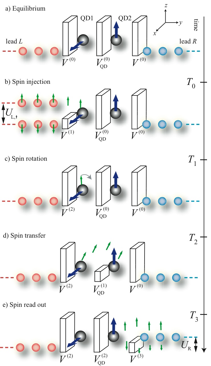
Figure 1: Schematic of the double quantum dot device coupled to leads. At $t<T_{0}=0$ the system is in equilibrium. At $T_{0}$ a spin bias $U_{L,\uparrow}$ is switched on and simultaneously the barrier between QD1 and the left lead is lowered. The injection of spin up electrons ends at $T_{1}$ when the bias is turned off and the barrier is raised up. Now the spin in QD1 rotates till $T_{2}$ when the barrier between the dots is lowered and the electron spin is transfer from QD1 to QD2. At $T_{3}$ the interdot barrier is raised up again while the barrier between QD2 and the right lead is lowered. Tuning the electrochemical potential in the right lead $U_{R}$ to be in between the two levels of QD2, we measure a large (small) spin current if the electron spin is parallel (antiparallel) to the spin impurity.

We consider a double quantum dot device to manipulate the spin orientation of spin-polarized electrons. Both quantum dots contain a static spin impurity with which the electron spin is coupled. The exchange coupling constant is much larger than experimentally accessible Larmor frequencies, a feature that renders the spin impurity a potentially ultrafast mean to rotate the electron spin.cl.2007 ; kkr.2007 Model systems of quantum transport through magnetic quantum dots have been previously used to study the conductance oscillations of a local nuclear spin in a magnetic field,zb.2002 the gauge-invariant nature of the charge and spin conductances,zc.2005 the spin-interference and Aharonov-Bohm oscillations in a quantum ring with embedded magnetic impurities,jsj.2001 ; atz.2005 ; cpz.2007 and the effects of the entanglement of two spin impurities on the conductance.cpzov.2006 ; cpzov.2007

In this paper we focus on the short time response of the system when subject to a sequence of voltage pulses, as illustrated in Fig. 1. The injection of spin polarized electrons from the left lead to the first quantum dot (QD1) is followed by a rotation of the electron spin in QD1. Afterwards the electron spin is transferred from QD1 to the second quantum dot (QD2) and its polarization is maintained parallel/antiparallel to the spin impurity of QD2. Eventually, the electron spin in QD2 is read out by calculating the spin current at the interface with the right lead. We provide a time-dependent description of some crucial processes in the theory of spin transport, namely the injection of spins from a lead to a quantum dot and the spin dynamics of a double quantum dot system weakly coupled to leads. The results of our analysis include 1) an overshooting of the spin accumulation during the spin injection phase, 2) a considerable delay in the spin relaxation for different exchange couplings in QD1 and QD2, and 3) oscillations in the transient regime whose frequency depends on the bandwidth of the leads and, therefore, are absent in the commonly used wide band limit approximation.

The paper is organized as follows. In Section II we present our model system and introduce the basic notation. A set of approximate equations to describe different operating processes are derived in Section III. We obtain a rate equation for the electron spin of a quantum dot in contact with an electron reservoir and identify the mechanisms leading to a deterioration of the spin polarization and to a damping of the spin magnitude. This analysis will then be used to optimize the spin injection from one of the leads to one of the quantum dots. We also investigate the spin transfer between the two quantum dots for different initial orientations of the electron spin. In Section IV we use a spin-generalized and modified version of the algorithm of Ref. ksarg.2005, , see Appendix B, to perform numerical simulations of the microscopic electron dynamics of the double quantum dot system. The results are then interpreted and discussed using the framework developed in Section III. In Section V we summarize the main findings and discuss future directions.

II Model system

We consider a basic two spin-impurities model consisting of two one-dimensional leads coupled to two single-level (per spin) quantum dots. The first quantum dot is connected to the left lead ($L$), the second quantum dot is connected to the right lead ($R$) and a hopping term accounts for tunneling of electrons between QD1 and QD2, see Fig. 1. The Hamiltonian describing the left ($L$) and right ($R$) leads is

$$H_{\alpha} = \sum_{\sigma=\uparrow,\downarrow}\sum_{j=0}^{\infty}\left[Vc^{{\dagger}}_{j\alpha,\sigma}c_{j+1\alpha,\sigma}+V^{\ast}c^{{\dagger}}_{j+1\alpha,\sigma}c_{j\alpha,\sigma}\right],$$ (1)

$$+ \sum_{\sigma=\uparrow,\downarrow}\varepsilon_{\alpha,\sigma}(t)\sum_{j=0}^{\infty}c^{{\dagger}}_{j\alpha,\sigma}c_{j\alpha,\sigma}$$

with $\alpha=L,R$. In Eq. (1) the quantity $V$ is the hopping integral between nearest neighbors orbitals and $\varepsilon_{\alpha,\sigma}(t)$ is the time-dependent on-site energy of lead $\alpha$ which, in general, can depend on spin. For $\varepsilon_{\alpha,\sigma}=0$ the energy window of both $L$ and $R$ continua is $(-2|V|,2|V|)$ and the half-filled system correspond to a chemical potential $\mu_{\rm hf}=0$. The Hamiltonian of the double quantum dot system reads

$$H_{\rm QD} = \sum_{i=1}^{2}\left[J_{i}\vec{S}_{i}\cdot\sum_{\sigma\sigma^{\prime}}d^{{\dagger}}_{i,\sigma}\vec{\sigma}_{\sigma\sigma^{\prime}}d_{i,\sigma^{\prime}}+v_{i}(t)\sum_{\sigma}d^{{\dagger}}_{i,\sigma}d_{i,\sigma}\right]$$ (2)

$$+ \sum_{\sigma}\left[V_{\rm QD}(t)d^{{\dagger}}_{1,\sigma}d_{2,\sigma}+V_{\rm QD}^{\ast}(t)d^{{\dagger}}_{2,\sigma}d_{1,\sigma}\right]$$

with $\vec{S}_{i}=(\sin\theta_{i}\cos\phi_{i},\sin\theta_{i}\sin\phi_{i},\cos\theta_{i})$ the spin of the impurity $i=1,2$, $J_{i}>0$ the corresponding antiferromagnetic exchange coupling, and $\vec{\sigma}=(\sigma_{x},\sigma_{y},\sigma_{z})$ the Pauli matrices. The tunnel barrier between the dots can be tuned by varying an external gate voltage.ldv.1998 This is modelled by using time-dependent gate voltages $v_{1}(t)$, $v_{2}(t)$ and interdot hopping integral $V_{\rm QD}(t)$. The first term in Eq. (2) is the Hamiltonian of the two isolated QDs and can conveniently be rewritten in matrix form as

$$\sum_{i=1}^{2}(d^{{\dagger}}_{i,\uparrow},d^{{\dagger}}_{i,\downarrow})\left(\begin{array}[]{cc}v_{i}+J_{i}\cos\theta_{i}&J_{i}e^{i\phi_{i}}\sin\theta_{i}\\ J_{i}e^{-i\phi_{i}}\sin\theta_{i}&v_{i}-J_{i}\cos\theta_{i}\end{array}\right)\left(\begin{array}[]{c}d_{i,\uparrow}\\ d_{i,\downarrow}\end{array}\right).$$ (3)

From Eq. (3) we see that the isolated QD has two levels at energy $\varepsilon_{i,\pm}=v_{i}\pm J_{i}$. If $J_{i}>|v_{i}|$ and $\varepsilon_{\alpha,\sigma}=0$ one level is above $\mu_{\rm hf}$ while the other is below.

The double QD system is connected to the left and right leads via the tunneling Hamiltonian

$$H_{T} = \sum_{\sigma}\left[V_{L}(t)d^{{\dagger}}_{1,\sigma}c_{0L,\sigma}+V_{L}^{\ast}(t)c^{{\dagger}}_{0L,\sigma}d_{1,\sigma}\right]$$ (4)

$$+ \sum_{\sigma}\left[V_{R}(t)d^{{\dagger}}_{2,\sigma}c_{0R,\sigma}+V_{R}^{\ast}(t)c^{{\dagger}}_{0R,\sigma}d_{2,\sigma}\right].$$

As for the interdot coupling $V_{\rm QD}$ we allow the hopping integrals $V_{L}(t)$ and $V_{R}(t)$ to be time-dependent.

Below we discuss a sequence of operations to manipulate the orientation of the electron spin in QD2 for a fixed orientation of the spin of the injected electrons. Without loss of generality we assume that for negative times, $t<0$, the whole system is in equilibrium at chemical potential $\mu$ and inverse temperature $\beta$ [Fig.1a)].c.1980 The two quantum dots are initially very weakly coupled to the leads, $V_{\alpha}<<V$, and between them, $V_{\rm QD}<<V$. Furthermore, the two energy levels of both QD1 and QD2 are much larger than the chemical potential, i.e., $\varepsilon_{i,\pm}>>\mu$, and the population on the dots is practically zero. Starting from this configuration we apply a sequence of four perturbations to 1) inject spin up electrons on QD1 [Fig.1b)] 2) rotate the electron spin in QD1 [Fig.1c)] 3) transfer the electron spin from QD1 to QD2 [Fig.1d)] and 4) read out the polarization of the electron spin in QD2 [Fig.1e)]. Due to the wide range of possible time-dependent perturbations we restrict the analysis to piece-wise constant (in time) parameters and obtain a set of approximate equations to study the four different processes. This study will then help us in selecting the parameters for target-specific numerical calculations. Full simulations of the entire sequence will be shown in Section IV.

III Theoretical Framework

III.1 Spin injection and spin read-out

At time $t=0$ we inject spin-up electrons into QD1 by suddenly switching on a spin bias,ls.2008 $\varepsilon_{L,\sigma}(t)=\theta(t)U_{L,\sigma}$, and reducing the height of the barrier between lead $L$ and QD1, i.e., $V_{L}(t)=\theta(-t)V^{(0)}+\theta(t)V^{(1)}$. The injection process terminates by switching off the spin bias and raising up the barrier to the equilibrium value $V^{(0)}$. There are two different mechanisms which contaminate the spin-up injection with $x$ and $y$ components. The first is the spin-precession around the spin impurity $\vec{S}_{1}$ while the second is the spin-relaxation due to the increased electron hopping $V_{L}$. To tackle this problem we take advantage of the fact that QD1 and QD2 are, during this process, weakly linked and we only consider the electron dynamics on QD1 in contact with the left reservoir, i.e., we approximate $V_{\rm QD}=0$. Using the non-equilibrium Green’s function formalism one finds the following equation for the lesser Green function $G^{<}_{\sigma\sigma^{\prime}}$ on QD1

$$i\frac{{\rm d}}{{\rm d}t}\mbox{\boldmath$G$}^{<}(t;t)=[\mbox{\boldmath$H$}_{\rm QD1},\mbox{\boldmath$G$}^{<}(t;t)]+\int_{0}^{\infty}{\rm d}\bar{t}$$

$$\times\left[\mbox{\boldmath$\Sigma$}_{L}^{<}(t;\bar{t})\mbox{\boldmath$G$}^{\rm A}(\bar{t};t)+\mbox{\boldmath$\Sigma$}_{L}^{\rm R}(t;\bar{t})\mbox{\boldmath$G$}^{<}(\bar{t};t)+{\rm h.c.}\right],$$ (5)

where we use boldface to indicate $2\times 2$ matrices in spin space and the symbol “$[,]$” denotes a commutator. In the above equation $\mbox{\boldmath$H$}_{\rm QD1}=v_{1}+J_{1}\vec{S}_{1}\cdot\vec{\sigma}$ is the one-particle Hamiltonian of the isolated QD1 while $\mbox{\boldmath$\Sigma$}_{L}$ is the embedding self-energy of lead $L$. We have discarded the integral between 0 and $-i\beta$ along the imaginary time axis since $V_{L}(t<0)=V^{(0)}<<V$ and hence $\mbox{\boldmath$\Sigma$}_{L}\sim 0$ in equilibrium.sa.2004 The superscripts R/A in $\mbox{\boldmath$\Sigma$}_{L}$ and $G$ denote retarded/advanced components. The self-energy is diagonal in spin space since there is no spin-flip hopping between lead $L$ and QD1. In terms of one-particle eigenstates $\psi_{k}(j)$ and eigenenergies $\varepsilon_{k}$ of lead $L$ one finds for $t,t^{\prime}>0$

$$\Sigma_{L,\sigma\sigma^{\prime}}^{\rm R}(t;t^{\prime}) = \delta_{\sigma\sigma^{\prime}}|V^{(1)}|^{2}\int\frac{{\rm d}\omega}{2\pi}e^{-i(\omega+U_{L,\sigma})(t-t^{\prime})}$$ (6)

$$\times \sum_{k}\frac{|\psi_{k}(0)|^{2}}{\omega-\varepsilon_{k}+i\eta},$$

$$\Sigma_{L,\sigma\sigma^{\prime}}^{<}(t;t^{\prime}) = \delta_{\sigma\sigma^{\prime}}|V^{(1)}|^{2}\int\frac{{\rm d}\omega}{2\pi}e^{-i(\omega+U_{L,\sigma})(t-t^{\prime})}if(\omega)$$ (7)

$$\times 2\pi\sum_{k}|\psi_{k}(0)|^{2}\delta(\omega-\varepsilon_{k}).$$

At low temperatures and low biases only frequencies close to the Fermi energy $\varepsilon_{\rm F}$ are probed. Using the Wide Band Limit (WBL) approximation, i.e.,

$$\sum_{k}|\psi_{k}(0)|^{2}\delta(\omega-\varepsilon_{k})\sim\rho_{\rm F}$$ (8)

with $\rho_{\rm F}=\rho(\varepsilon_{\rm F})$ the local density of states at the interface, we can approximate Eqs. (6-7) as

$$\Sigma_{L,\sigma\sigma^{\prime}}^{\rm R}(t;t^{\prime})=-\frac{i}{2}\delta_{\sigma\sigma^{\prime}}\Gamma\delta(t-t^{\prime}),$$ (9)

$$\Sigma_{L,\sigma\sigma^{\prime}}^{\rm<}(t;t^{\prime})=i\delta_{\sigma\sigma^{\prime}}\Gamma\int\frac{{\rm d}\omega}{2\pi}e^{-i(\omega+U_{L,\sigma})(t-t^{\prime})}f(\omega)$$

$$\simeq-\delta_{\sigma\sigma^{\prime}}\frac{\Gamma}{2\pi}e^{-i\varepsilon_{\rm F,\sigma}(t-t^{\prime})}\left[\frac{1}{t-t^{\prime}}-i\pi\delta(t-t^{\prime})\right],$$ (10)

with $\Gamma=2\pi|V^{(1)}|^{2}\rho_{\rm F}$ and $\varepsilon_{\rm F,\sigma}=\varepsilon_{\rm F}+U_{L,\sigma}$. In Eq. (10) we have further approximated $\mbox{\boldmath$\Sigma$}^{<}_{L}$ with its expression at zero temperature.

Inserting these results into Eq. (5) one obtains

$$i\frac{{\rm d}}{{\rm d}t}\mbox{\boldmath$G$}^{<}(t;t)=[\mbox{\boldmath$H$}_{\rm QD1},\mbox{\boldmath$G$}^{<}(t;t)]-\frac{i}{2}\{\mbox{\boldmath$\Gamma$},\mbox{\boldmath$G$}^{<}(t;t)\}$$

$$-\mbox{\boldmath$\Gamma$}-\left[\frac{\mbox{\boldmath$\Gamma$}}{2\pi}\int_{0}^{t}{\rm d}\bar{t}\,\frac{\exp[-i\mbox{\boldmath$\mathcal{E}$}_{\rm F}(t-\bar{t})]}{t-\bar{t}}\mbox{\boldmath$G$}^{\rm A}(\bar{t};t)+{\rm h.c.}\right],$$ (11)

where the symbol “$\{,\}$” denotes the anticommutator and the matrices $[\mbox{\boldmath$\Gamma$}]_{\sigma\sigma^{\prime}}=\delta_{\sigma\sigma^{\prime}}\Gamma$ and $[\mbox{\boldmath$\mathcal{E}$}_{\rm F}]_{\sigma\sigma^{\prime}}=\delta_{\sigma\sigma^{\prime}}\varepsilon_{\rm F,\sigma}$. From Eq. (11) we can extract a rate equation for the electron spin

$$\vec{S}_{1,\rm el}(t)\equiv-\frac{i}{2}{\rm Tr}\left[\mbox{\boldmath$G$}^{<}(t;t)\vec{\sigma}\right]$$ (12)

on QD1. In the WBL approximation the advanced Green’s function reads

$$\mbox{\boldmath$G$}^{\rm A}(\bar{t};t) = i\theta(-\Delta t)\exp[-i(\mbox{\boldmath$H$}_{\rm QD1}+\frac{i}{2}\mbox{\boldmath$\Gamma$})\Delta t]$$ (13)

$$= i\theta(-\Delta t)e^{-i(v_{1}+\frac{i}{2}\Gamma)\Delta t}$$

$$\times \left[\cos(J_{1}\Delta t)-i\sin(J_{1}\Delta t)\vec{S}_{1}\cdot\vec{\sigma}\right],$$

with $\Delta t\equiv\bar{t}-t$. Substituting this result into Eq. (11), multiplying with $\vec{\sigma}$ and tracing over the spin indices we find

$$\frac{{\rm d}}{{\rm d}t}\vec{S}_{1,\rm el} = J_{1}(\vec{S}_{1}\wedge\vec{S}_{1,\rm el})-\frac{\Gamma}{2}\vec{S}_{1,\rm el}$$

$$- \frac{\Gamma}{\pi}\int_{0}^{t}\frac{{\rm d}\bar{t}}{\Delta t}\,e^{\frac{\Gamma}{2}\Delta t}\cos((\varepsilon_{+}-v_{1})\Delta t)$$

$$\times [\cos(\varepsilon_{-}\Delta t)\sin(J_{1}\Delta t)\vec{S}_{1}$$

$$- \sin(\varepsilon_{-}\Delta t)\{\cos(J_{1}\Delta t)\hat{z}-\sin(J_{1}\Delta t)\hat{z}\wedge\vec{S}_{1}\}],$$

with $\hat{z}$ the unit vector in the $z$ direction, and $\varepsilon_{\pm}=\varepsilon_{\rm F,\uparrow}\pm\varepsilon_{\rm F,\downarrow}$. It is instructive to expand the right hand side in powers of $t$. To first order in $t$ one finds a simplified rate equation for the electron spin

$$\frac{{\rm d}}{{\rm d}t}\vec{S}_{1,\rm el}=J_{1}(\vec{S}_{1}\wedge\vec{S}_{1,\rm el})-\frac{\Gamma}{2}\vec{S}_{1,\rm el}+\frac{t}{\pi}\left(\Gamma\varepsilon_{-}\hat{z}-J_{1}\Gamma\vec{S}_{1}\right),$$ (15)

which is reliable for times $t^{-1}\geq\max[\varepsilon_{-},J_{1}]/2\pi$. From the above equation we can identify four different contributions. The term proportional to $\hat{z}$ is the spin-injection term and is responsible for an increase of the electron spin along the $z$ direction. Such increase is quadratic in time and faster the larger the difference $\varepsilon_{-}=U_{L,\uparrow}-U_{L,\downarrow}$ is. The first and the last terms are responsible for a deterioration of the spin direction due to spin precession (first term) and spin relaxation (last term). The latter drives the electron spin towards a configuration antiparallel to the spin impurity $\vec{S}_{1}$. Finally, the second term is responsible for an overall damping of the spin magnitude. Going beyond the first order in $t$, see Eq. (LABEL:sre), one observes the appearance of a new relaxation direction, that is $\hat{z}\wedge\vec{S}_{1}$. This latter result is completely general as it is only dictated by the symmetry of the system.

We wish to emphasize that the rate equation (LABEL:sre) has been derived under the sole assumption that the quantum dot QD1 is initially isolated and then contacted with lead $L$. This is the same situation occurring in the spin read-out phase when the barrier between the weakly coupled QD2 and lead $R$ is lowered. Thus, the rate equation for $\vec{S}_{2,\rm el}$ during the read-out phase is identical to Eq. (LABEL:sre) for $\vec{S}_{1,\rm el}$ even though the parameters are different and, more importantly, different initial conditions must be imposed.

III.2 Spin rotation and spin transfer

After a time $T_{1}$ the spin bias is switched off and the hopping $V_{L}$ is again reduced to values much smaller than $V$. In this phase QD1 is well isolated and the electron spin precesses around the spin impurity $\vec{S}_{1}$ according to

$$\frac{{\rm d}}{{\rm d}t}\vec{S}_{1,\rm el}=J_{1}(\vec{S}_{1}\wedge\vec{S}_{1,\rm el}),\quad t>T_{1}.$$ (16)

Let us now specialize to the situation illustrated in Fig. 1 with $\vec{S}_{1}$ oriented along the positive $x$ axis and $\vec{S}_{2}$ along the positive $z$ axis. We recall that the Fermi energy is much smaller than the energy levels of the two isolated quantum dots and hence that the equilibrium electron density is vanishingly small. For $J_{1}>>\varepsilon_{-}$, see Eq. (15), we expect an efficient injection of spin up electrons in QD1 and for $J_{1}>>\Gamma$ a major contamination along the $y$ direction. This implies that the electron spin $\vec{S}_{1,\rm el}(T_{1})$ has a small $x$ component at the end of the spin injection process. Since $\vec{S}_{1}$ is parallel to the $x$ axis $\vec{S}_{1,\rm el}(t)$ rotates in the $yz$ plane for $t>T_{1}$. We let the system evolve till a time $T_{2}>T_{1}$ and we approximate $\vec{S}_{1,\rm el}(T_{2})=(0,S_{1,\rm el}^{y}(T_{2}),S_{1,\rm el}^{z}(T_{2}))$ on the $yz$ plane and $\vec{S}_{2,\rm el}(T_{2})=0$ (this latter approximation comes from the fact that $V_{\rm QD}$ and $V_{R}$ are both much smaller than $V$ for $t<T_{2}$).

At $t=T_{2}$ we transfer the electron spin by lowering the barrier between QD1 and QD2. This corresponds to an increase of the interdot hopping $V_{\rm QD}$. Letting $|\Phi(T_{2})\rangle$ be the evolved many-particle state of the entire system at $t=T_{2}$, the density matrix $\rho$ of the double quantum dot system has matrix elements $[\mbox{\boldmath$\rho$}]_{i\sigma,j\sigma^{\prime}}=\langle\Phi(T_{2})|d^{{\dagger}}_{j,\sigma^{\prime}}d_{i,\sigma}|\Phi(T_{2})\rangle$. It is convenient to introduce the notation $1=(1,\uparrow)$, $2=(1,\downarrow)$, $3=(2,\uparrow)$ and $4=(2,\downarrow)$ for the collective index $(i,\sigma)$. The density matrix is then represented by the following $4\times 4$ matrix

$$\mbox{\boldmath$\rho$}=2S_{1,\rm el}(T_{2})\left(\begin{array}[]{cccc}\cos^{2}\theta&-\frac{i}{2}\sin 2\theta&0&0\\ \frac{i}{2}\sin 2\theta&\sin^{2}\theta&0&0\\ 0&0&0&0\\ 0&0&0&0\end{array}\right),$$ (17)

with $\sin 2\theta=S_{1,\rm el}^{y}(T_{2})/S_{1,\rm el}(T_{2})$, $\cos 2\theta=S_{1,\rm el}^{z}(T_{2})/S_{1,\rm el}(T_{2})$, and $S_{1,\rm el}=\sqrt{\vec{S}_{1,\rm el}\cdot\vec{S}_{1,\rm el}}$ the spin magnitude. We are interested in how to choose the angle $\theta$ in order to maximize the electron spin of QD2 along the $z$ direction (parallel/antiparallel to the spin impurity $\vec{S}_{2}$). For simplicity we take the gate voltages $v_{1}=0$ and $v_{2}=0$. Then the isolated double quantum dot system is described by the $4\times 4$ Hamiltonian matrix

$$\mbox{\boldmath$H$}_{\rm QD}=\left(\begin{array}[]{cc}J_{1}\sigma_{x}&V_{\rm QD}\mbox{\boldmath$1$}_{2}\\ V_{\rm QD}\mbox{\boldmath$1$}_{2}&J_{2}\sigma_{z}\end{array}\right),$$ (18)

with $\mbox{\boldmath$1$}_{2}$ the $2\times 2$ identity matrix. In terms of $\rho$ and $\mbox{\boldmath$H$}_{\rm QD}$ the $z$ component $S^{z}_{2,\rm el}$ of the electron spin on QD2 is given by

$$S^{z}_{2,\rm el}(t+T_{2})=\frac{1}{2}{\rm Tr}\left[\mbox{\boldmath$\Sigma$}_{2}^{z}\exp(i\mbox{\boldmath$H$}_{\rm QD}t)\mbox{\boldmath$\rho$}\exp(-i\mbox{\boldmath$H$}_{\rm QD}t)\right],$$ (19)

with the spin operator of QD2

$$\mbox{\boldmath$\Sigma$}_{2}^{z}=\left(\begin{array}[]{cc}\mbox{\boldmath$0$}_{2}&\mbox{\boldmath$0$}_{2}\\ \mbox{\boldmath$0$}_{2}&\sigma_{z}\end{array}\right),$$ (20)

and $\mbox{\boldmath$0$}_{2}$ the $2\times 2$ null matrix. Substituting $\rho$ from Eq. (17) we find

$$\frac{S^{z}_{2,\rm el}(t+T_{2})}{S_{1,\rm el}(T_{2})} = \frac{i}{2}\sin 2\theta\left\{[\mbox{\boldmath$\Sigma$}_{2}^{z}(t)]_{1,2}-[\mbox{\boldmath$\Sigma$}_{2}^{z}(t)]_{2,1}\right\}$$

$$+ \cos^{2}\theta[\mbox{\boldmath$\Sigma$}_{2}^{z}(t)]_{1,1}+\sin^{2}\theta[\mbox{\boldmath$\Sigma$}_{2}^{z}(t)]_{2,2},$$

where we have defined the spin operator in the Heisenberg representation

$$\mbox{\boldmath$\Sigma$}_{2}^{z}(t)\equiv\exp(-i\mbox{\boldmath$H$}_{\rm QD}t)\mbox{\boldmath$\Sigma$}_{2}^{z}\exp(i\mbox{\boldmath$H$}_{\rm QD}t).$$ (22)

It is easy to prove that the function $O(t)\equiv\frac{i}{2}([\mbox{\boldmath$\Sigma$}_{2}^{z}(t)]_{1,2}-[\mbox{\boldmath$\Sigma$}_{2}^{z}(t)]_{2,1})$ is an odd function of time while $[\mbox{\boldmath$\Sigma$}_{2}^{z}(t)]_{1,1}$ and $[\mbox{\boldmath$\Sigma$}_{2}^{z}(t)]_{2,2}$ are even functions of time. In appendix A we further prove that

$$E(t)\equiv[\mbox{\boldmath$\Sigma$}_{2}^{z}(t)]_{1,1}=-[\mbox{\boldmath$\Sigma$}_{2}^{z}(t)]_{2,2},$$ (23)

which leads to the simple formula

$$S^{z}_{2,\rm el}(t+T_{2}) = S_{1,\rm el}(T_{2})[O(t)\sin 2\theta+E(t)\cos 2\theta]$$ (24)

$$= O(t)S^{y}_{1,\rm el}+E(t)S^{z}_{1,\rm el}.$$

The function $E(t)$ can be written as a linear combination of the cosine functions $\cos(\omega_{\mu\nu}t)$ while $O(t)$ as a linear combination of the sine functions $\sin(\omega_{\mu\nu}t)$, where $\omega_{\mu\nu}=\varepsilon_{\mu}-\varepsilon_{\nu}$ is the difference between two eigenvalues of $\mbox{\boldmath$H$}_{\rm QD}$. The eigenvalues $\varepsilon_{\mu}$, $\mu=1,\ldots,4$ can be calculated analytically and read

$$\varepsilon_{\mu}=\pm\sqrt{\frac{J_{+}^{2}+2V_{\rm QD}^{2}\pm\sqrt{J_{-}^{4}+4J_{+}^{2}V_{\rm QD}^{2}}}{2}},$$ (25)

with $J^{2}_{\pm}=J_{1}^{2}\pm J_{2}^{2}$.

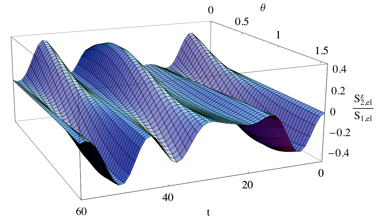
Figure 2: Ratio $S^{z}_{2,\rm el}(t+T_{2})/S_{1,\rm el}(T_{2})$ versus time $t$ and initial polarization $\theta$ for $J_{1}=J_{2}=0.1$ and $V_{\rm QD}=0.2$.

As an example, in Fig. 2 we plot the ratio $S^{z}_{2,\rm el}(t+T_{2})/S_{1,\rm el}(T_{2})$ as a function of time $t$ and initial polarization $\theta$ for $J_{1}=J_{2}=0.1$ and $V_{\rm QD}=0.2$. We notice that for most polarizations $S^{z}_{2,\rm el}(t+T_{2})$ remains smaller than $0.2$. Only for some special value of $\theta$ the $z$ component of the spin in QD2 reaches a value larger than 0.4. This means that the maximum efficiency in transferring an electron spin polarized in the $yz$ plane from QD1 to QD2 with final polarization along the positive $z$ axis is about $80-90\%$.

All above processes can be numerically simulated without resorting to any of the approximations employed in this Section. This allows for a more quantitative investigation of the device performance and will be the topic of the next Section.

IV Numerical simulations and discussion

In this Section we use a modified version of the algorithm proposed in Ref. ksarg.2005, to propagate in time finite systems in contact with infinitely long leads, see Appendix B, and investigate the microscopic dynamics of the spin-injection, the spin-accumulation as well as the spin rotation of conducting electrons scattering against the double QD device of Eq. (2). In the following analysis energies are measured in units of $V$, times in units of $\hbar/V$, spins in units of $\hbar$ and currents in units of $eV/\hbar$, with $e$ the electron charge. The full Hamiltonian is time independent for negative times and the system is in equilibrium at zero temperature and Fermi energy $\varepsilon_{\rm F}$.c.1980 We start by considering two identical QDs with exchange coupling $J_{1}=J_{2}=0.1$ and gate potential $v_{1}=v_{2}=0$ weakly coupled to the left and right leads, $V_{L}=V_{R}=V^{(0)}=0.01$, and with interdot hopping $V_{\rm QD}=0.01$. Choosing $V\sim 100$ meV the exchange couplings $J_{1},J_{2}\sim 10$ meV lie in the physical parameter rangekkr.2007 and the corresponding time unit is $\hbar/V\sim 100$ fs which is appropriate to study ultrafast dynamics.gksa.2001 ; mklsa.2007 The impurity spin $\vec{S}_{1}$ of QD1 is oriented along the positive $x$ axis while $\vec{S}_{2}$ is oriented along the positive $z$ axis. The on-site energies of the leads $\varepsilon_{\alpha,\sigma}$ are initially all zero.

IV.1 Spin injection

At time $t=0$ we switch on a spin bias $\varepsilon_{L,\uparrow}(t)=\theta(t)U_{L,\uparrow}$ in lead $L$ for spin up electrons ($U_{L,\downarrow}=0$) and increase the hopping $V_{L}$ from $V^{(0)}$ to $V^{(1)}$.

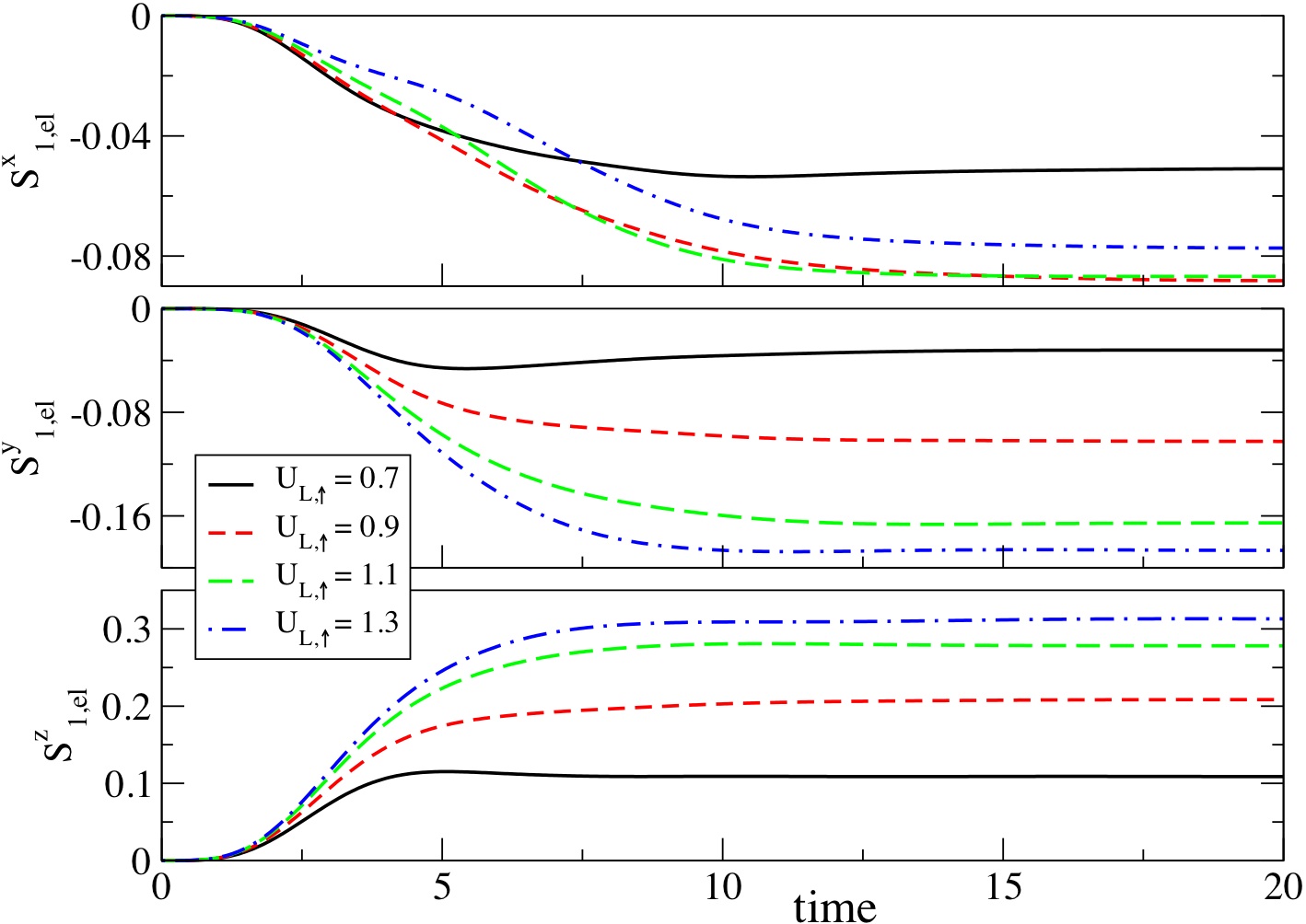
Figure 3: The three components of the electron spin in QD1 versus time for a sudden change of the hopping $V_{L}$ from $V^{(0)}=0.01$ to $V^{(1)}=0.5$ and a simultaneous sudden switching of the spin-bias $U_{L,\uparrow}=0.7,\;0.9,\;1.1,\;1.3$. The equilibrium parameters are $J_{1}=J_{2}=0.1$, $V_{L}=V_{R}=V_{\rm QD}=V^{(0)}$ and the Fermi energy is $\varepsilon_{\rm F}=0.96$.

In Fig. 3 we study the spin-injection process when the Fermi energy is $\varepsilon_{\rm F}=-0.96$ (which correspond to an initial electron occupation on QD1 of the order of $10^{-5}$) and the hopping between $L$ and QD1 at positive times is $V^{(1)}=0.5$. We calculate the time-dependent expectation value of the spin of the conducting electrons $\vec{S}_{1,{\rm el}}$ on QD1 for different biases $U_{L,\uparrow}$. Since $U_{L,\uparrow}\sim 1>J_{1}$ the rate equation (15) is reliable for times $t\leq 2\pi/U_{L,\uparrow}\sim 2\pi$. In this time window we observe that the $z$ component $S_{1,{\rm el}}^{z}$ increases quadratically in time and that the rate is larger the larger is the spin bias $U_{L,\uparrow}$, in agreement with Eq. (15) (we recall that in this case $\varepsilon_{-}=U_{L,\uparrow}$). The $y$ component $S_{1,{\rm el}}^{y}$ has a trend similar to $S_{1,{\rm el}}^{z}$ but the transient is even smoother. This can be explained by observing that as the spin up electrons enter QD1 they undergo a spin rotation due to the spin impurity oriented along the positive $x$ axis. Taking into account that for small $t$ we have $S_{1,{\rm el}}^{z}\sim t^{2}$, from Eq. (15) we see that $S_{1,{\rm el}}^{y}\sim J_{1}t^{3}$. As the $z$ component also the $x$ component $S_{1,{\rm el}}^{x}$ grows quadratically in time. From Eq. (15) one finds $S_{1,{\rm el}}^{z}(t)/S_{1,{\rm el}}^{x}(t)\sim\varepsilon_{-}/J_{1}$ meaning that to minimize the contamination of spin up electrons with an $x$ component it must be $\varepsilon_{-}/J_{1}>1$.

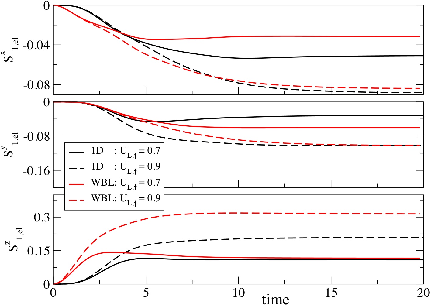
Figure 4: Comparison between the results obtained with one-dimensional (1D) leads and WBL leads for the electron spin in QD1 and $U_{L,\uparrow}=0.7,\;0.9$. The other parameters are the same as in Fig. 3.

We wish to observe that at intermediate biases $U_{L,\uparrow}$ the numerical results agree with the rate equation (LABEL:sre) only qualitatively. The comparison between the time evolution of the electron spin in QD1 for $U_{L,\uparrow}=0.7,\;0.9$ as obtained with one-dimensional leads and with leads treated in the WBL approximation is shown in Fig. 4.

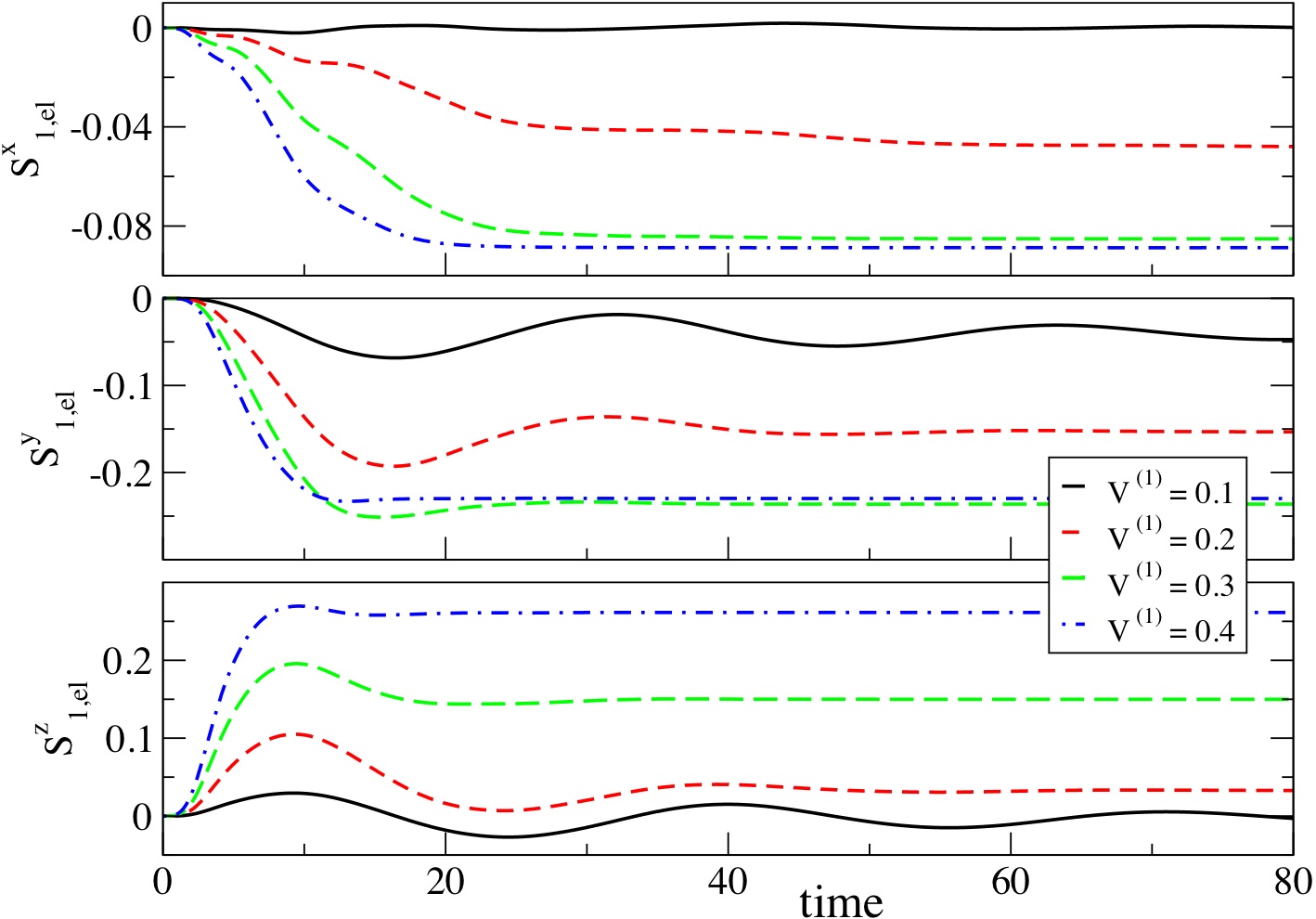
Figure 5: The three components of the electron spin in QD1 versus time for a sudden switching of the spin-bias $U_{L,\uparrow}=1.3$ and a simultaneous sudden change of the hopping $V_{L}$ from $V^{(0)}=0.01$ to $V^{(1)}=0.1,\;0.2,\;0.3,\;0.4$. The other parameters are the same as in Fig. 3.

In Fig. 5 we fix the bias for spin-up electrons to be $U_{L,\uparrow}=1.3$ and analyze the spin-dynamics on QD1 for different values of $V^{(1)}$. We first observe that the transient time decreases by increasing $V^{(1)}$ and hence $\Gamma$. This is easily understood by noticing that the second term in Eq. (LABEL:sre) yields an exponential damping of the spin oscillations. The spin oscillations can be observed in the $y$ and $z$ components and are due to the spin precession around the spin impurity $\vec{S}_{1}$. The period of the oscillation is $T=\pi/J_{1}$ and is independent of $V^{(1)}$, as it should. It is also interesting to observe that for small times $S_{1,{\rm el}}^{z}$ overshoots its steady value and hence more efficient spin injections may be achieved by properly engineering the transient response. In our case, for an efficient spin up injection only the ratios $r_{xy}=|S_{1,{\rm el}}^{x}/S_{1,{\rm el}}^{y}|$ and $r_{xz}=|S_{1,{\rm el}}^{x}/S_{1,{\rm el}}^{z}|$ must be small at the end of the process since the $y$ component can be reduced to zero in the second phase when $V_{L}<<V$ and $\vec{S}_{1,\rm el}$ can precess around the spin impurity. From Fig. 5 we find that for $V_{\rm par}=0.2$ and at $t\sim 10$ the ratios $r_{xy}\sim 0.1$ and $r_{xz}\sim 0.12$ while at the steady state $r_{xy}\sim 0.31$ and $r_{xz}\sim 1.43$.

IV.2 Spin rotation

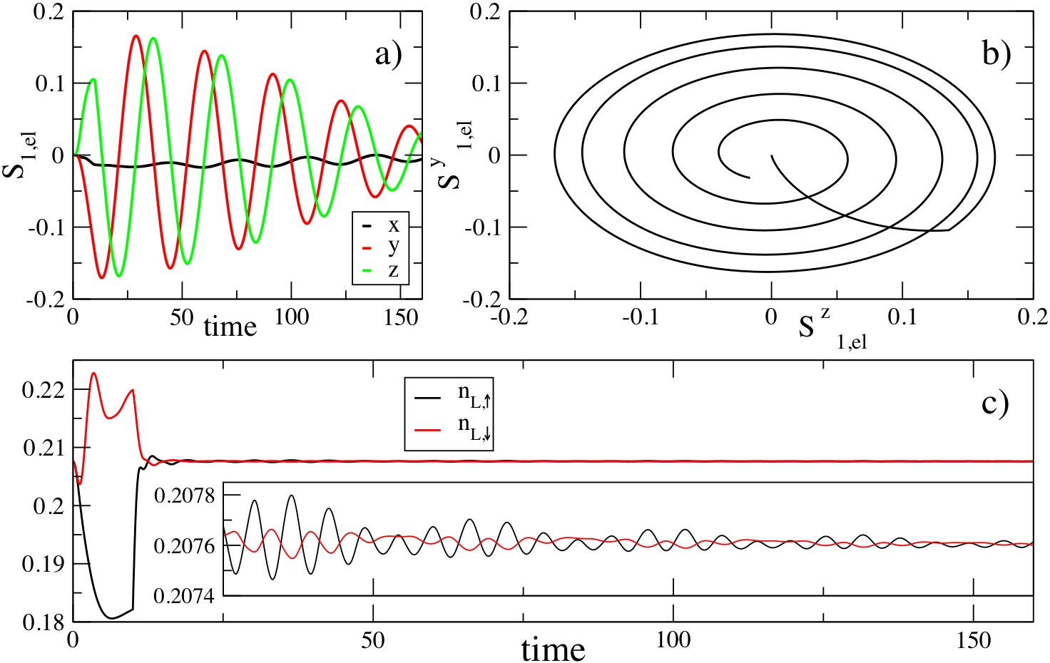
Figure 6: Electron spin in QD1 and electron density at the left interface during the injection phase ($t<T_{1}$) and the rotation phase ($t>T_{1}$) when $T_{1}=10$. The equilibrium parameters are the same as in Fig. 5, i.e., $J_{1}=J_{2}=0.1$, $V_{L}=V_{R}=V_{\rm QD}=V^{(0)}$ and the Fermi energy is $\varepsilon_{\rm F}=0.96$. For $0<t<T_{1}$ the system is perturbed by a spin bias $U_{L,\uparrow}=1.3$ and a larger hopping $V_{L}=V^{(1)}=0.2$. At $t=T_{1}$ the spin bias is switched off and the hopping $V_{L}$ is suddenly changed to $V^{(2)}=0.01$. Panel a) The three components of $\vec{S}_{1,\rm el}$. Panel b) The trajectory of the projection of $\vec{S}_{1,\rm el}$ onto the $yz$ plane. Panel c) Spin up and down density on the first site of the left lead. The inset is a magnification of both densities $n_{L,\uparrow}$ and $n_{L\downarrow}$ for times $t>25$.

The injection process terminates after some time $T_{1}$ by switching the spin bias off and raising back the barrier between QD1 and the left lead, i.e., $V_{L}(t)=\theta(-t)V^{(0)}+\theta(t)\theta(T_{1}-t)V^{(1)}+\theta(t-T_{1})V^{(2)}$. During the second phase QD1 is weakly coupled to the environment and the electron spin precesses around $\vec{S}_{1}$. Let us focus on the situation discussed above with $V^{(1)}=0.2$ and let $T_{1}=10$ be the duration of the first phase. In Fig. 6 we study the electron spin on QD1 [panels a) and b)] and the densities $n_{L,\sigma}\equiv\langle c^{{\dagger}}_{0L,\sigma}c_{0L,\sigma}\rangle$ on the first site of the left electrode [panel c)] for $V^{(2)}=0.01$. The contaminating component $S_{1,\rm el}^{x}$ ceases to decrease at $t=T_{1}$ while the $y$ and $z$ components are well described by damped cosine functions with a phase lag of $\pi/(4J_{1})$ [panel a)]. Due to the weak contact $V^{(2)}$ the magnitude $S_{1,\rm el}=\sqrt{\vec{S}_{1,\rm el}\cdot\vec{S}_{1,\rm el}}$ of the electron spin changes on a time scale much longer than the spin-exchange time-scale $\sim 1/J_{1}$. This is shown in panel b) where the trajectory of $\vec{S}_{1,\rm el}$ is projected onto the $yz$ plane. For times $t<T_{1}$ the trajectory has a large radial component while for $t>T_{1}$ the spin moves along a spiral trajectory. It is also interesting to look at the densities on the nearest neighbor site of QD1 [panel c)]. During the first phase ($t<T_{1}$) a majority of spin up electrons are transferred from lead $L$ to QD1 and, as a consequence, $n_{L,\uparrow}$ decreases. On the contrary the density $n_{L,\downarrow}$ increases due to the following two-step mechanism. As the spin up electrons hop from lead $L$ to QD1 they undergo a spin rotation and acquire a down component. These electrons have about zero energy and can easily hop to the left lead where the spin-down band is filled up to $\varepsilon_{\rm F}+U_{L,\downarrow}=\varepsilon_{\rm F}=-0.96$. At the end of the injection process the densities change abruptly and approach their initial value since $V^{(2)}=V^{(0)}$. The inset of panel c) is a magnification of the curves $n_{L,\uparrow}(t)$ and $n_{L,\downarrow}(t)$ for $25<t<160$. It is clearly visible a quantum beating in both densities due to the alignment of the spin impurity along the $x$ axis. In both cases two oscillations with frequency $|\varepsilon_{\rm F}\pm J_{1}|=0.96\pm 0.1$ are superimposed to an envelope oscillation of frequency $2J_{1}=0.2$.

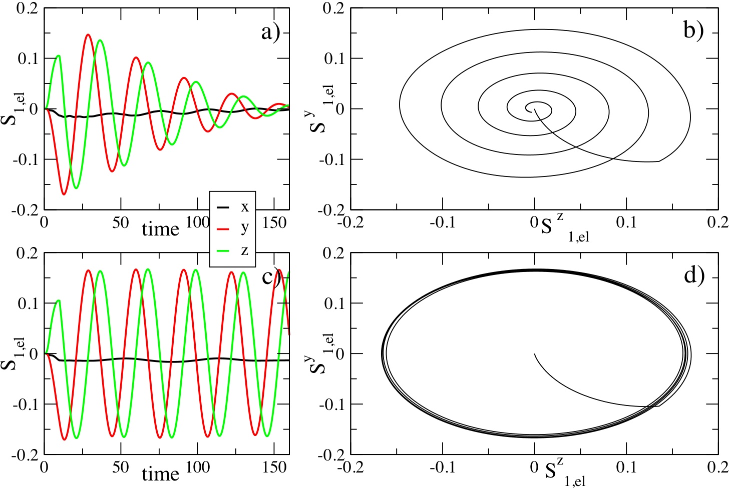
Figure 7: The three components of $\vec{S}_{1,\rm el}$ [panel a)] and the trajectory of the projection of $\vec{S}_{1,\rm el}$ onto the $yz$ plane [panel b)] for the same system as in Fig. 6 except that the hopping parameter $V^{(2)}=0.06$ is six times larger. Panels c)-d) like panels a)-b) but the equilibrium parameter $J_{2}=0.02$ while the hopping parameter $V^{(2)}=0.01$.

The spin rotation phase is further investigated in Fig. 7 where we consider the same system as in Fig. 6 except for the value of the hopping parameter $V^{(2)}=0.06$ which is six times larger [panels a) and b)] or the exchange coupling $J_{2}=0.02$ which is five times smaller [panels c) and d)]. In the first case the $x$ component remains an order of magnitude smaller than $S_{1,\rm el}$ [see panel a)] and eventually approaches a steady value slightly larger than the initial one [not shown]. As in Fig. 6 the electron spin is damped in all three directions but it decays faster. The projection of $\vec{S}_{1,\rm el}$ onto the $yz$ plane [panel b)] yields a spiral trajectory which finishes very close to the origin after a time $t\sim 160$. On the other hand, for a smaller coupling $J_{2}=J_{1}/5$ we do not appreciate any damping within the time propagation window $t<160$. The $y$ and $z$ components of $\vec{S}_{1,\rm el}$ are well described by two undamped cosine functions with a phase lag $\pi/(4J_{1})$ and an amplitude which is about ten times larger than $|S^{x}_{1,\rm el}|$, see panel c). In panel d) we show the projection of $\vec{S}_{1,\rm el}$ onto the $yz$ plane. The reduced damping is a desirable feature and has to be attributed to the mismatch of the energy levels in the two quantum dots: $\pm J_{1}$ in QD1 and $\pm J_{2}$ in QD2.

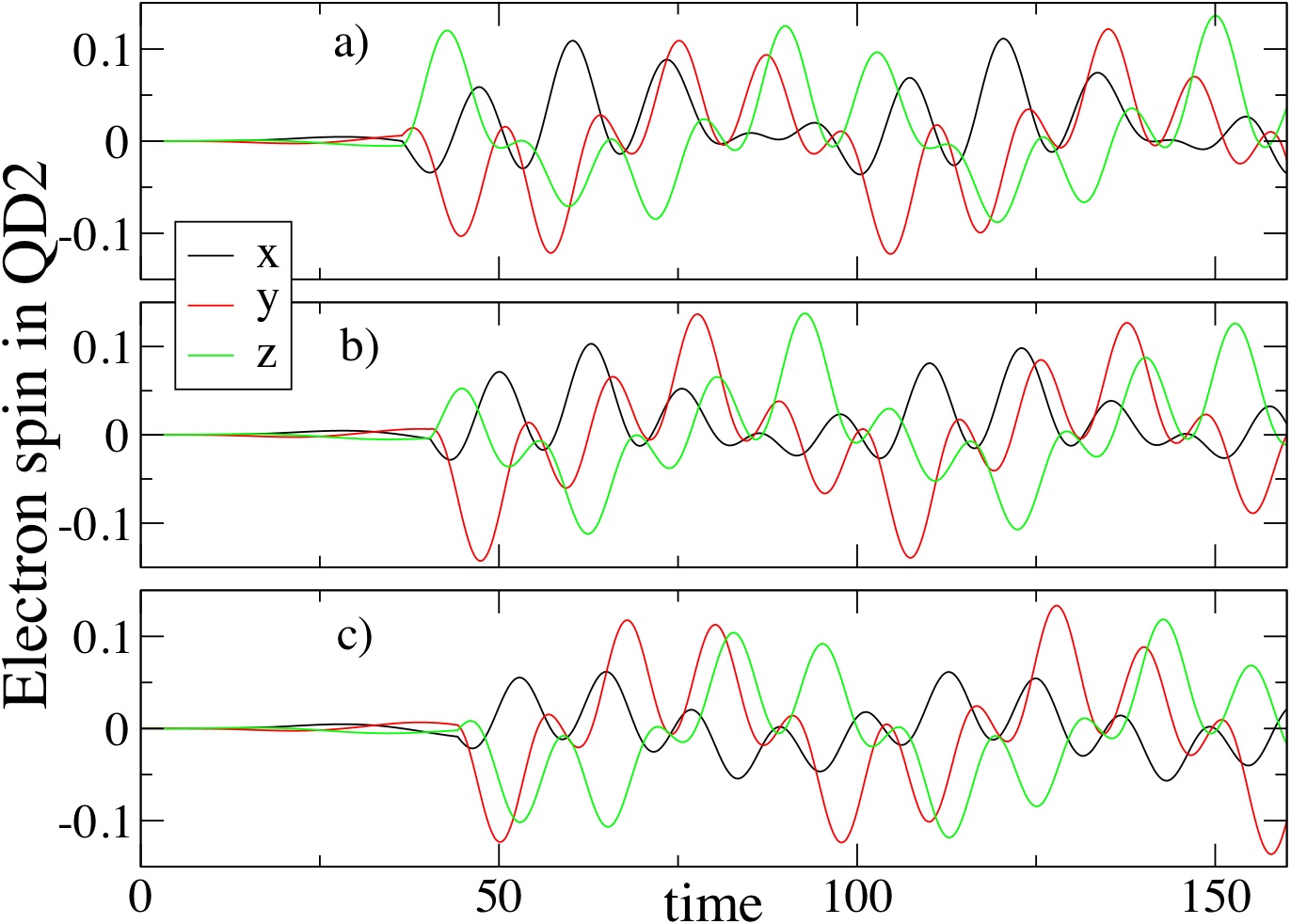
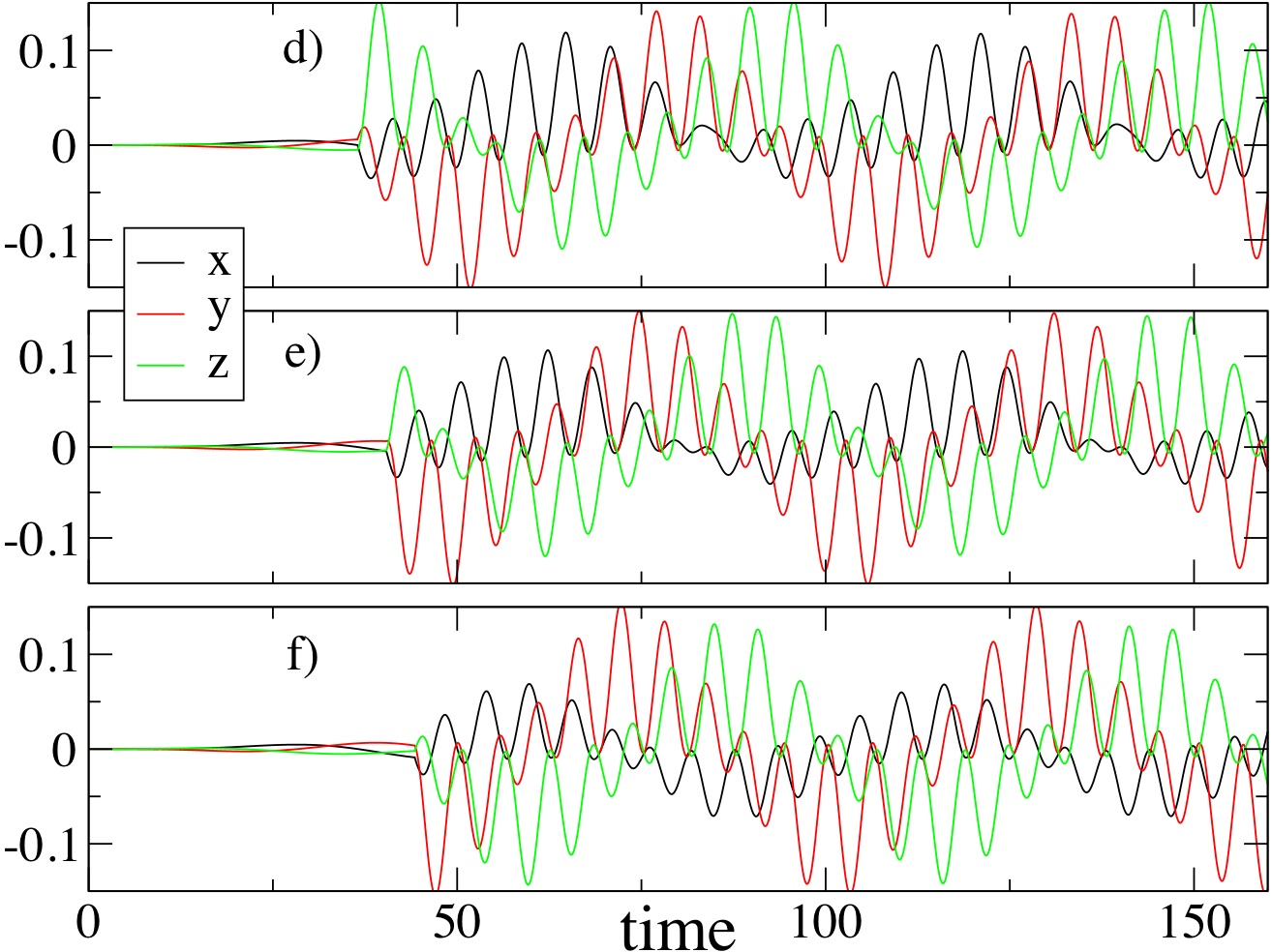
Figure 8: The electron spin $\vec{S}_{2,\rm el}$ in QD2 before ($t<T_{2}$) and after ($t>T_{2}$) the spin transfer phase when the interdot hopping is set to $V_{\rm QD}^{(1)}=0.2$ [panels a) to c)] and $V_{\rm QD}^{(1)}=0.5$ [panels d) to f)]. The transfer phase starts at $T_{2}\sim 36.5$ [panels a) and d)], $T_{2}\sim 40.4$ [panels b) and e)], and $T_{2}\sim 44.3$ [panels c) and f)]. All parameters before time $T_{2}$ are the same as in Fig. 6 except for the exchange coupling $J_{2}=0.05$.

IV.3 Spin transfer

The rotation of the electron spin in QD1 ($t>T_{1}$) terminates at $t=T_{2}>T_{1}$ when the barrier between QD1 and QD2 is lowered and, as a consequence, the interdot hopping increases, i.e., $V_{\rm QD}=V_{\rm QD}^{(0)}\theta(T_{2}-t)+V_{\rm QD}^{(1)}\theta(t-T_{2})$, where $V_{\rm QD}^{(0)}=0.01$. This is the spin transfer phase. In Fig. 8 we plot the three components of the electron spin in QD2 versus time for $V_{\rm QD}^{(1)}=0.2$ [panels a) to c)] and $V_{\rm QD}^{(1)}=0.5$ [panels d) to f)]. For times $t<T_{2}$ the system undergoes the same perturbations as in Figs. 6-7. Here we have considered an exchange coupling in QD2 of $J_{2}=0.05$ and a hopping $V^{(2)}=0.01$. The frequency of the oscillations is larger the larger the interdot coupling is, in agreement with Eq. (25). The efficiency of the transfer has been investigated for different times $T_{2}$ at which the electron spin in QD1 is polarized along $\hat{z}$ [$T_{2}\sim 36.5$, panels a) and d)], $\frac{1}{\sqrt{2}}(\hat{z}-\hat{y})$ [$T_{2}\sim 40.4$, panels b) and e)], and $-\hat{y}$ [$T_{2}\sim 44.3$, panels c) and f)]. For our choice of parameters the efficiency is higher if the spin in QD1 is polarized along $\hat{z}$.

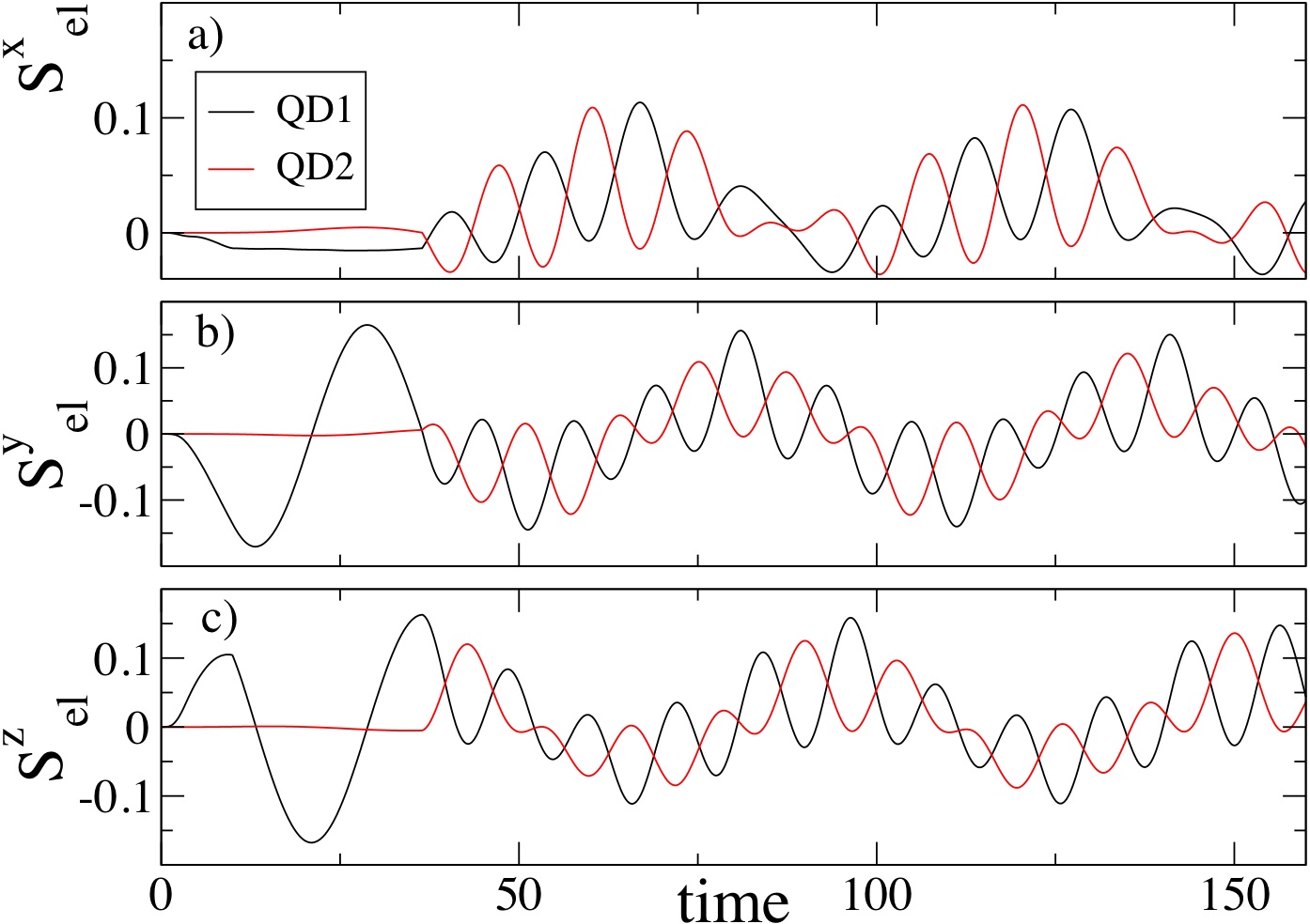
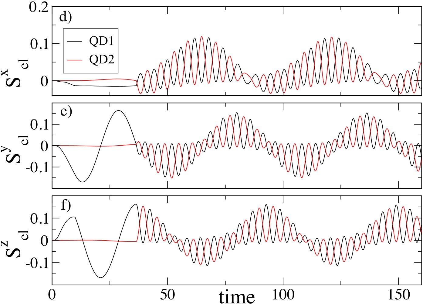
Figure 9: Electron spin in QD1 and QD2 for $T_{2}=36.5$ and $V_{\rm QD}^{(1)}=0.2$ [panels a) to c)] and $V_{\rm QD}^{(1)}=0.5$ [panels d) to f)]. The other parameters are the same as in Fig. 8.

We also observe that for all three components the maxima of the electron spin in QD1 correspond to the minima of the electron spin in QD2, see Fig. 9 where we plot $\vec{S}_{1,\rm el}$ and $\vec{S}_{2,\rm el}$ for $T_{2}=36.5$ and $V_{\rm QD}^{(1)}=0.2$ [panels a) to c)] and $V_{\rm QD}^{(1)}=0.5$ [panels d) to f)]. From Fig. 8 panel d) and Fig. 9 panels d) to f) one observes that when $T_{2}$ corresponds to the time at which $\vec{S}_{1,\rm el}(T_{2})$ is polarized along $\hat{z}$, the maxima of $S^{z}_{2,\rm el}$ are close to the zeros of $S^{x}_{2,\rm el}$ and $S^{y}_{2,\rm el}$, in agreement with the analysis of Section III.2. We define the ratio $r_{\perp}\equiv S^{z}_{2,\rm el}/\sqrt{(S^{x}_{2,\rm el})^{2}+(S^{y}_{2,\rm el})^{2}}$. In the propagation window the maxima of $S^{z}_{2,\rm el}$ occur at $t=39.32$ when $r_{\perp}\sim 0.28$ and $S^{z}_{2,\rm el}=0.153$, $t=95.68$ when $r_{\perp}\sim 0.26$ and $S^{z}_{2,\rm el}=0.152$, and $t=151.96$ when $r_{\perp}\sim 0.24$ and $S^{z}_{2,\rm el}=0.151$. Taking into account that $S^{z}_{1,\rm el}(T_{2})=0.163$ the efficiency of the spin transfer can be up to $90\%$.

IV.4 Spin read out

At a time $t=T_{3}$ when $S^{z}_{2,\rm el}$ has a maximum or a minimum, the interdot hopping is lowered, i.e., $V_{\rm QD}(t)=V_{\rm QD}^{(0)}\theta(T_{2}-t)+V_{\rm QD}^{(1)}\theta(t-T_{2})\theta(T_{3}-t)+V_{\rm QD}^{(2)}\theta(t-T_{3})$ with $V_{\rm QD}^{(2)}<<V$, and the spin transfer phase ends.

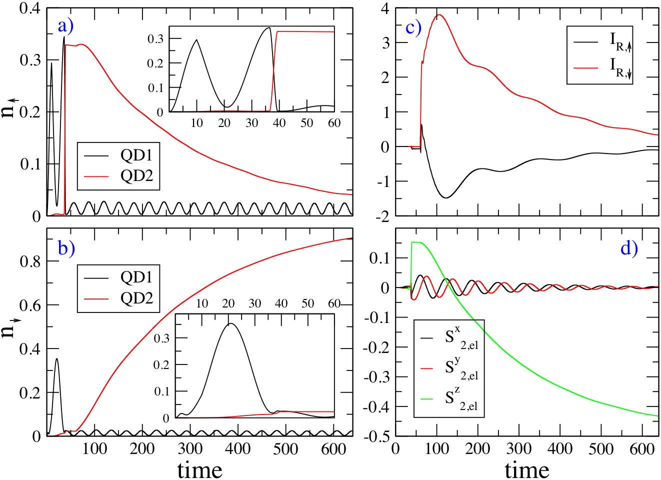
Figure 10: Spin up density [panel a)] and spin down density [panel b)] in QD1 and QD2 (the inset shows a magnification of the time window $0<t<60$). The spin polarized current at the right interface, $I_{R,\sigma}(t)$, is displayed in panel c) in units of $10^{-3}$, while panel d) shows $\vec{S}_{2,\rm el}(t)$. For $t<T_{3}=39.32$ the system parameters and the perturbations are the same as in Fig. 9 with $V_{\rm QD}^{(1)}=0.5$. For $t\geq T_{3}$ the interdot hopping is lowered to the value $V_{\rm QD}^{(2)}=0.001$ and QD2 becomes a well isolated system. At $t=60>T_{3}$ the hopping $V_{R}(t)$ between QD2 and lead $R$ is raised up to $V^{(3)}=0.05$ and simultaneously a bias $U_{R,\uparrow}=U_{R,\downarrow}=0.96$ is switched on in the right lead. At this time the electrochemical potential in lead $R$ is $\mu_{R}=\varepsilon_{\rm F}+0.96=0$ and lies in between the two spin levels of QD2.

In Fig. 10 we consider the same system parameters and perturbations of Fig. 9 (with $V_{\rm QD}^{(1)}=0.5$) and fix the time $T_{3}=39.32$ when $S^{z}_{2,\rm el}$ has a maximum. At $t=T_{3}$ the interdot hopping is lowered to $V_{\rm QD}^{(2)}=0.001$ and QD2 becomes an almost isolated system. At this stage the density of spin up and down electrons in QD2 is practically constant as one can see from the insets of Fig. 10 in panels a) and b). Shortly after $T_{3}$ the read out phase starts. At $t=60$ we lower the barrier between QD2 and lead $R$ and simultaneously switch on a bias $U_{R,\uparrow}=U_{R,\downarrow}=U_{R}=0.96$ in the right lead. The electrochemical potential in lead $R$ becomes $\mu_{R}=\varepsilon_{\rm F}+U_{R}=0$ and lies in between the two energy levels $\varepsilon_{2,\pm}=\pm J_{2}=\pm 0.05$ of the isolated QD2, with the highest level $\varepsilon_{2,+}$ for spin up electrons and the lowest level $\varepsilon_{2,-}$ for spin down electrons.note Spin up electrons in QD2 have, therefore, energy larger than $\mu_{R}$ and tunnel to the lead $R$. As a consequence the spin up density decreases, as one can see in Fig. 10 panel a). On the contrary, the lowest level $\varepsilon_{2,-}$ has energy below $\mu_{R}$ and a vanishingly small occupation. Spin down electrons tunnel from lead $R$ to QD2 and the density of spin down electrons increases, see Fig. 10 panel b). This charge transfer generates a right-going spin-up current $I_{R,\uparrow}$ and a left-going spin-down current $I_{R,\downarrow}$, see Fig. 10 panel c), which results in a large spin-current. The spin dynamics in the $xy$ plane is displayed in Fig. 10 panel d) where, besides the monotonically decreasing $z$ component, we plot the $x$ and $y$ components of $\vec{S}_{2,\rm el}$. Due to the symmetry of the problem $S^{x}_{2,\rm el}$ and $S^{y}_{2,\rm el}$ oscillate around zero with an exponentially decreasing amplitude.

Figure 11: Spin up density [panel a)] spin down density [panel b)] on QD1 and QD2, spin polarized current at the right interface, $I_{R,\sigma}$, in units of $10^{-3}$ [panel c)], and $\vec{S}_{2,\rm el}$ [panel d)]. The insets of panels a)-b) show a magnification of the density in the time window $0<t<60$. Same system parameters and perturbations of Fig. 10 but $T_{2}=52.05$ and $T_{3}=54.84$.

The situation corresponding to the antiparallel configuration in QD2 is analyzed in Fig. 11. The difference with the previous case is that we let the electron spin in QD1 rotate till is polarized along the negative $z$ axis. The first time $S^{z}_{1,\rm el}$ is minimum occurs at $T_{2}=52.05$, see insets in panels a) and b). The spin transfer phase ends at $T_{3}=54.84$ with an efficiency of about $90\%$. This can be seen in the inset of panel b) where the spin down density of QD2 swaps with that of QD1 in the time window $(T_{2},T_{3})$. At $t=T_{3}$ the system undergoes the same perturbations considered in Fig. 10. Being the spin up level of QD2 scarcely populated the change in the spin up density [panel a)] and spin up current at the right interface [panel c)] is very small as compared to the parallel configuration. A small change is observed for the spin down quantities as well due to a population of about 0.3 in the spin down level of QD2. Contrary to the parallel configuration set up, the $z$ component $S^{z}_{2,\rm el}$ is negative when the read out phase starts and does not change sign, see panel d).

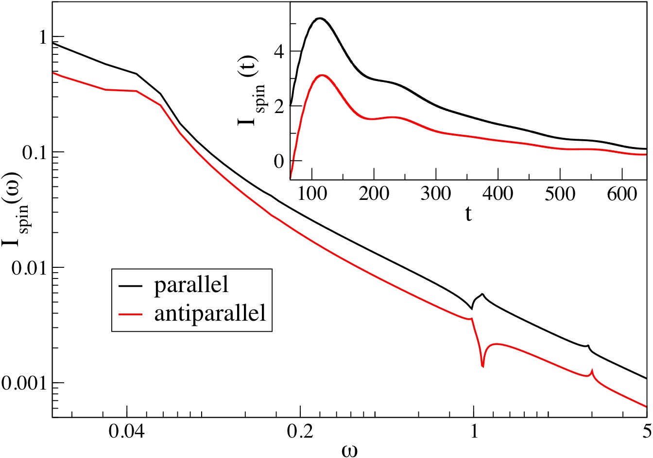
Figure 12: Discrete Fourier transform of the spin current $I_{\rm spin}=I_{R,\downarrow}-I_{R,\uparrow}$ at the right interface for the parallel and antiparallel configurations of Fig. 10 and Fig. 11 respectively. The inset shows $I_{\rm spin}$ in time domain, with $t$ in the range (65, 640), which has been used to perform the discrete Fourier transform. Both $I_{\rm spin}(\omega)$ and $I_{\rm spin}(t)$ are in units of $10^{-3}$.

The spin current $I_{\rm spin}(t)\equiv I_{R,\downarrow}(t)-I_{R,\uparrow}(t)$ during the read-out phase ($t>60$) is displayed in the inset of Fig. 12 for the parallel and antiparallel configurations analyzed in Figs. 10-11. One observes an exponential decay with superimposed oscillations of frequency $|\varepsilon_{\rm F}+U_{R}\pm J_{2}|=0.05$, as expected. However, a closer inspection reveals a richer structure. In Fig. 12 we show the discrete Fourier transform of $I_{\rm spin}(t)$ with $t$ in the range $(65,640)$. Besides the peak at $\omega=0.05$ there exist an extra peak at frequency $\omega=|2-\varepsilon_{\rm F}|\sim 2.96$ and an asymmetric peak structure at frequency $\omega=|\varepsilon_{\rm F}+2|\sim 1.04$. The extra transient frequencies are due to the finite bandwidth of the leads since the energies +2 and -2 (in units of $V$) correspond the top and the bottom of the right band.

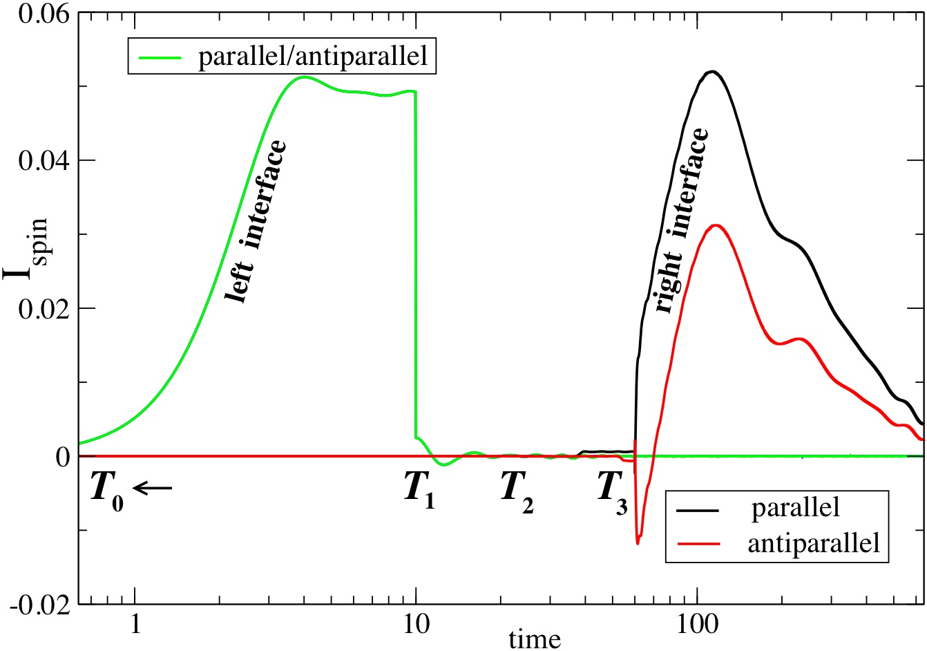
Figure 13: Spin current at the left and right interfaces for the parallel and antiparallel configurations of Fig. 10 and Fig. 11 respectively. For the parallel configuration $T_{0}=0$, $T_{1}=10.0$, $T_{2}=36.5$, and $T_{3}=39.32$, while for the antiparallel configuration $T_{0}=0$, $T_{1}=10.0$, $T_{2}=52.05$, and $T_{3}=54.84$.

In conclusion, we have shown how to propagate in time a spinful open quantum system subject to arbitrary time- and spin-dependent perturbations. The semi-infinite nature of the leads has been exactly accounted for. Full simulations of the microscopic charge and spin transient dynamics of a double quantum dot in its operating regime have been presented. Figure 13 summarizes how the device works by displaying the spin currents at the left and right interfaces during the entire sequence of voltage pulses. Different processing of the injected spin up current results in different spin currents at the right interface.

V Summary and Outlook

In the last few years we have witnessed an increasing interest on transient responses in quantum transport mainly due to their potential relevancy in molecular electronics, a field where molecular devices will possibly operate under non-steady-state conditions. The main difficulty in the study of the short-time response of open quantum systems stems from the macroscopic size of the leads. Several approaches have been proposed to tackle this problem. Treating the leads in the WBL approximation allows for obtaining a simple integral equation for currents, densities, etc.,jmw.1994 ; sl.1997.1 ; ylz.2000 ; zwymc.2007 but lacks retardation effects. One-dimensional leads have been approximately treated within a Wigner-function approachf.1990 ; dn.2005 or by including only a finite number of lead unit-cells.ds.2006 ; as.2007 ; bsdv.2005 Only recently it became possible to deal with the semi-infinite nature of the leads using a scheme based on wave-functions propagationksarg.2005 or, alternatively, other algorithms based on solving the Dyson-Keldysh equations in the time-domain.zmjg.2005 ; hhlkch.2006 ; mwg.2006 ; mgm.2007 ; hhlhc.2007 Few attempts to include electron-correlationsl.1997.2 ; ktt.2001 as well as electron-nuclear interactionsvsa.2006 ; sssbht.2006 in the transient regime have also been made.

In this work we have used a modified version of the propagation algorithm of Ref. ksarg.2005, , see Appendix B, and generalized it to include the spin degrees of freedom. We have proposed a double quantum dot system to manipulate the charge and the spin of the electrons. Numerical simulations of the entire operating regime have been provided. These include some of the crucial steps in the theory of quantum computation, like, e.g., the injection of spins and their read out.

The transient electron dynamics when a device is perturbed by ultrafast voltage pulses is not only relevant to our microscopic understanding but an exploitable feature to improve the device performance. This has been explicitly shown in Section IV: the efficiency of the spin injection can be much higher during the transient than at the steady state. We also have found that for a given height of the barriers between lead $L$ and QD1, QD1 and QD2, and QD2 and lead $R$, the damping of the spin magnitude during the rotation phase is much smaller for different exchange couplings, i.e., $J_{1}\neq J_{2}$, than for $J_{1}=J_{2}$. This means that the spin relaxation can be substantially delayed using different quantum dots.

Using the non-equilibrium Green’s function formalism in the WBL approximation we have obtained a rate equation for both the spin-injection and spin read-out processes. For short times the rate equation becomes remarkably transparent and permits us to identify the mechanisms leading to a relaxation of the spin magnitude and to a deterioration of the spin polarization. Going beyond the WBL approximation results in a richer structure of the transient responses, as transitions between the Fermi energy and the bottom/top of the band occur as well.

As shown in Section IV, the possibility of simulating operational sequences like, e.g., that of Fig. 1, allows for a real-time study of fundamental processes not accessible otherwise. Much more work is, however, needed before a systematic comparison with experimental data can be made. Accounting for intradot and possibly interdot electron-electron interactions is of crucial importance for describing, e.g., the Coulomb blockade or the Kondo regimes. The complications here stem from the necessity of including electron correlations in a time-dependent conserving manner, a progress which can be made either within the framework of many body theoryb.1962 or within one-particle frameworks like, e.g., time-dependent density functional theory.rg.1984 ; vbdvls.2005 Developments in this direction have been made in steady-state situations by treating the correlation at the GW level.tr.2007 ; dfmo.2007 ; wshm.2008 ; tr.2008

Another fundamental issue to be pursued is the extension to three-dimensional leads. This would allow for a proper treatment of the long-range Coulomb potential as well as for a realistic description of the atomistic structure of the tunneling barriers.

Finally, the recent experimental advances in attaching quantum dots to superconducting leadsbosht.2007 prompt for a generalization of the propagation algorithm to leads described by, e.g., BCS-like models. Such development will give us access to a completely new phenomenology due to the competition between the pairing interaction and the spin-flip interactions, a topic not yet explored in the transient regime.

Appendix A Proof of Eq. (23)

The result in Eq. (23) is a consequence of the relative orientation of the spin impurity $\vec{S}_{1}$ with respect to $\vec{S}_{2}$. By definition the quantity $[\mbox{\boldmath$\Sigma$}_{2}^{z}(t)]_{1,1}$ is the (1,1) matrix element of the product of three matrices

$$[\mbox{\boldmath$\Sigma$}_{2}^{z}(t)]_{1,1}=\left[e^{-it\left(\begin{array}[]{cc}J_{1}\sigma_{x}&V_{\rm QD}\mbox{\boldmath$1$}_{2}\\ V_{\rm QD}\mbox{\boldmath$1$}_{2}&J_{2}\sigma_{z}\end{array}\right)}\left(\begin{array}[]{cc}\mbox{\boldmath$0$}_{2}&\mbox{\boldmath$0$}_{2}\\ \mbox{\boldmath$0$}_{2}&\sigma_{z}\end{array}\right)e^{it\left(\begin{array}[]{cc}J_{1}\sigma_{x}&V_{\rm QD}\mbox{\boldmath$1$}_{2}\\ V_{\rm QD}\mbox{\boldmath$1$}_{2}&J_{2}\sigma_{z}\end{array}\right)}\right]_{1,1}.$$ (26)

Consider the unitary operator $\mbox{\boldmath$U$}=\mbox{\boldmath$U$}_{g}\mbox{\boldmath$U$}_{z}\mbox{\boldmath$U$}_{x}$ which consists of a rotation of both spin impurities around the $x$ axis by an angle $\pi$, $\mbox{\boldmath$U$}_{x}=\left(\begin{array}[]{cc}\exp[-i\pi\sigma_{x}/2]&\mbox{\boldmath$0$}_{2}\\ \mbox{\boldmath$0$}_{2}&\exp[-i\pi\sigma_{x}/2]\end{array}\right),$ followed by a rotation around the $z$ axis by an angle $\pi$, $\mbox{\boldmath$U$}_{z}=\left(\begin{array}[]{cc}\exp[-i\pi\sigma_{z}/2]&\mbox{\boldmath$0$}_{2}\\ \mbox{\boldmath$0$}_{2}&\exp[-i\pi\sigma_{z}/2]\end{array}\right),$ followed by a gauge transformation which changes the sign of the fermion operators on QD2, $\mbox{\boldmath$U$}_{g}=\left(\begin{array}[]{cc}\mbox{\boldmath$1$}_{2}&\mbox{\boldmath$0$}_{2}\\ \mbox{\boldmath$0$}_{2}&-\mbox{\boldmath$1$}_{2}\end{array}\right).$ Insertions of the identity matrix $\mbox{\boldmath$U$}^{{\dagger}}\mbox{\boldmath$U$}$ in Eq. (26) gives

$$[\mbox{\boldmath$\Sigma$}_{2}^{z}(t)]_{1,1} = \left[\mbox{\boldmath$U$}^{{\dagger}}\mbox{\boldmath$U$}e^{-it\left(\begin{array}[]{cc}J_{1}\sigma_{x}&V_{\rm QD}\mbox{\boldmath$1$}_{2}\\ V_{\rm QD}\mbox{\boldmath$1$}_{2}&J_{2}\sigma_{z}\end{array}\right)}\mbox{\boldmath$U$}^{{\dagger}}\mbox{\boldmath$U$}\left(\begin{array}[]{cc}\mbox{\boldmath$0$}_{2}&\mbox{\boldmath$0$}_{2}\\ \mbox{\boldmath$0$}_{2}&\sigma_{z}\end{array}\right)\mbox{\boldmath$U$}^{{\dagger}}\mbox{\boldmath$U$}e^{it\left(\begin{array}[]{cc}J_{1}\sigma_{x}&V_{\rm QD}\mbox{\boldmath$1$}_{2}\\ V_{\rm QD}\mbox{\boldmath$1$}_{2}&J_{2}\sigma_{z}\end{array}\right)}\mbox{\boldmath$U$}^{{\dagger}}\mbox{\boldmath$U$}\right]_{1,1}$$ (33)

$$= -\left[e^{it\left(\begin{array}[]{cc}J_{1}\sigma_{x}&V_{\rm QD}\mbox{\boldmath$1$}_{2}\\ V_{\rm QD}\mbox{\boldmath$1$}_{2}&J_{2}\sigma_{z}\end{array}\right)}\left(\begin{array}[]{cc}\mbox{\boldmath$0$}_{2}&\mbox{\boldmath$0$}_{2}\\ \mbox{\boldmath$0$}_{2}&\sigma_{z}\end{array}\right)e^{-it\left(\begin{array}[]{cc}J_{1}\sigma_{x}&V_{\rm QD}\mbox{\boldmath$1$}_{2}\\ V_{\rm QD}\mbox{\boldmath$1$}_{2}&J_{2}\sigma_{z}\end{array}\right)}\right]_{2,2}=-[\mbox{\boldmath$\Sigma$}_{2}^{z}(-t)]_{2,2}.$$ (40)

Taking into account that $[\mbox{\boldmath$\Sigma$}_{2}^{z}(t)]_{1,1}$, $[\mbox{\boldmath$\Sigma$}_{2}^{z}(t)]_{2,2}$ are even functions of $t$, Eq. (23) follows.

Appendix B Propagation Algorithm

Let $\mbox{\boldmath$H$}(t)=\sum_{\alpha}\mbox{\boldmath$H$}_{\alpha}(t)+\sum_{\alpha}(\mbox{\boldmath$H$}^{0}_{\alpha C}+\mbox{\boldmath$H$}^{0}_{C\alpha})+\mbox{\boldmath$H$}_{C}(t)$ be the one-particle Hamiltonian of a system which consists of $\alpha=1,2,\ldots,N$ electrodes in contact with a central region $C$. We assume that the time dependence of

$$\mbox{\boldmath$H$}_{\alpha}(t) = \left(\begin{array}[]{cc}\mbox{\boldmath$H$}_{\alpha,\uparrow}^{0}&\mbox{\boldmath$0$}\\ \mbox{\boldmath$0$}&\mbox{\boldmath$H$}_{\alpha,\downarrow}^{0}\end{array}\right)+\left(\begin{array}[]{cc}U_{\alpha,\uparrow}(t)&\mbox{\boldmath$0$}\\ \mbox{\boldmath$0$}&U_{\alpha,\downarrow}(t)\end{array}\right)$$ (45)

$$= \mbox{\boldmath$H$}_{\alpha}^{0}+\mbox{\boldmath$U$}_{\alpha}(t)$$ (46)

is a uniform spin-dependent and time-dependent shift while the time-dependence of $\mbox{\boldmath$H$}_{C}$ has no restrictions. We denote with $|\psi_{\alpha}\rangle$ the projection of a generic wave-function $|\psi\rangle$ on electrode $\alpha$ and with $|\psi_{C}\rangle$ the projection of $|\psi\rangle$ onto region $C$. The time-dependent Schrödinger equation reads

$$i\frac{{\rm d}}{{\rm d}t}|\psi_{\alpha}(t)\rangle=\mbox{\boldmath$H$}_{\alpha}(t)|\psi_{\alpha}(t)\rangle+\mbox{\boldmath$H$}^{0}_{\alpha C}|\psi_{C}(t)\rangle,$$ (47)

$$i\frac{{\rm d}}{{\rm d}t}|\psi_{C}(t)\rangle=\mbox{\boldmath$H$}_{C}(t)|\psi_{C}(t)\rangle+\sum_{\alpha}\mbox{\boldmath$H$}_{C\alpha}^{0}|\psi_{\alpha}(t)\rangle.$$ (48)

Performing the gauge transformation

$$|\psi_{\alpha}(t)\rangle=\exp[-i\int_{0}^{t}{\rm d}\tau\,\mbox{\boldmath$U$}_{\alpha}(\tau)]\,|\phi_{\alpha}(t)\rangle,$$ (49)

and $|\psi_{C}(t)\rangle=|\phi_{C}(t)\rangle$, Eqs. (47-48) become

$$i\frac{{\rm d}}{{\rm d}t}|\phi_{\alpha}(t)\rangle=\mbox{\boldmath$H$}_{\alpha}^{0}|\psi_{\alpha}(t)\rangle+\mbox{\boldmath$H$}_{\alpha C}(t)|\phi_{C}(t)\rangle,$$ (50)

$$i\frac{{\rm d}}{{\rm d}t}|\phi_{C}(t)\rangle=\mbox{\boldmath$H$}_{C}(t)|\phi_{C}(t)\rangle+\sum_{\alpha}\mbox{\boldmath$H$}_{C\alpha}(t)|\phi_{\alpha}(t)\rangle,$$ (51)

with $\mbox{\boldmath$H$}_{C\alpha}(t)=\mbox{\boldmath$H$}_{C\alpha}^{0}\exp[-i\int_{0}^{t}{\rm d}\tau\mbox{\boldmath$U$}_{\alpha}(\tau)]$ and $\mbox{\boldmath$H$}_{\alpha C}(t)=[\mbox{\boldmath$H$}_{C\alpha}(t)]^{{\dagger}}$. The effect of the gauge transformation is to transfer the time dependence from the Hamiltonian describing the bulk electrodes to the Hamiltonian describing the contacts between the electrodes and region $C$. The gauge-transformed Schrödinger equation is used to calculate the time evolved state $|\phi(t_{m}=m\Delta t)\rangle\equiv|\phi^{(m)}\rangle$ by using the Cayley method

$$(1+i\delta\mbox{\boldmath$H$}_{g}^{(m)})|\phi^{(m+1)}\rangle=(1-i\delta\mbox{\boldmath$H$}_{g}^{(m)})|\phi^{(m)}\rangle,$$ (52)

where $\delta=\Delta t/2$, $\mbox{\boldmath$H$}_{g}^{(m)}=\frac{1}{2}[\mbox{\boldmath$H$}_{g}(t_{m+1})+\mbox{\boldmath$H$}_{g}(t_{m})]$, and $\mbox{\boldmath$H$}_{g}(t)=\sum_{\alpha}\mbox{\boldmath$H$}_{\alpha}^{0}+\sum_{\alpha}(\mbox{\boldmath$H$}_{\alpha C}(t)+\mbox{\boldmath$H$}_{C\alpha}(t))+\mbox{\boldmath$H$}_{C}(t)$ is the gauge-transformed Hamiltonian. The interface Hamiltonian $\mbox{\boldmath$H$}_{\alpha C}$ is spin-diagonal provided region $C$ includes the first few atomic layers of electrode $\alpha$. In this case the projection of Eq. (52) onto different subregions leads to a close recursive relation for the amplitudes $|\phi_{C}^{(m)}\rangle$ of the wave-function in region $C$ (the steps are similar to those of Ref. ksarg.2005, )

$$|\phi^{(m+1)}_{C}\rangle=\frac{1-i\delta\mbox{\boldmath$H$}^{(m)}_{\rm eff}}{1+i\delta\mbox{\boldmath$H$}^{(m)}_{\rm eff}}|\phi^{(m)}_{C}\rangle+|S^{(m)}\rangle-|M^{(m)}\rangle$$ (53)

where the source term $|S^{(m)}\rangle$ and the memory term $|M^{(m)}\rangle$ read

$$|S^{(m)}\rangle=\frac{-2i\delta}{1+i\delta\mbox{\boldmath$H$}^{(m)}_{\rm eff}}\sum_{\alpha}\mbox{\boldmath$z$}_{\alpha}^{(m)}\mbox{\boldmath$H$}_{C\alpha}^{0}\frac{(1-i\delta\mbox{\boldmath$H$}^{0}_{\alpha})^{m}}{(1+i\delta\mbox{\boldmath$H$}^{0}_{\alpha})^{m+1}}|\phi_{\alpha}^{(0)}\rangle,$$ (54)

$$|M^{(m)}\rangle = \frac{\delta^{2}}{1+i\delta\mbox{\boldmath$H$}^{(m)}_{\rm eff}}\sum_{\alpha}\sum_{j=0}^{m-1}\mbox{\boldmath$z$}_{\alpha}^{(m)}(\mbox{\boldmath$Q$}_{\alpha}^{(j)}+\mbox{\boldmath$Q$}_{\alpha}^{(j+1)})$$ (55)

$$\times \bar{\mbox{\boldmath$z$}}_{\alpha}^{(m-1-j)}(|\phi_{C}^{(m-j)}\rangle+|\phi_{C}^{(m-1-j)}\rangle).$$

In the above equations we have used the following definitions

$$\mbox{\boldmath$z$}_{\alpha}^{(m)}=\frac{\exp[-i\int_{0}^{t_{m+1}}{\rm d}\tau\,\mbox{\boldmath$U$}_{\alpha}(\tau)]+\exp[-i\int_{0}^{t_{m}}{\rm d}\tau\,\mbox{\boldmath$U$}_{\alpha}(\tau)]}{2},$$ (56)

$$\mbox{\boldmath$Q$}_{\alpha}^{(m)}=\mbox{\boldmath$H$}^{0}_{C\alpha}\frac{(1-i\delta\mbox{\boldmath$H$}^{0}_{\alpha})^{m}}{(1+i\delta\mbox{\boldmath$H$}^{0}_{\alpha})^{m+1}}\mbox{\boldmath$H$}^{0}_{\alpha C},$$ (57)

$$\mbox{\boldmath$H$}^{(m)}_{\rm eff}=\mbox{\boldmath$H$}_{C}^{(m)}-i\delta\sum_{\alpha}\mbox{\boldmath$z$}_{\alpha}^{(m)}\mbox{\boldmath$Q$}_{\alpha}^{(0)}\bar{\mbox{\boldmath$z$}}_{\alpha}^{(m)}.$$ (58)

The recursive relation in Eq. (53) is written in terms of matrices and vectors with the same dimension of the central region, i.e., the infinitely large electrodes have been embedded in an effective equation of finite dimension. We defer the reader to Ref. ksarg.2005, for the description of how to calculate the matrices $\mbox{\boldmath$Q$}_{\alpha}^{(m)}$ and the source term $|S^{(m)}\rangle$.

References

- (1) M. A. Nielsen and I. L. Chuang, Quantum Computation and Quantum Information, Cambridge University Press, Cambridge, England, 2000.
- (2) D. Awschalom, N. Samarth, and D. Loss, Semiconductor Spintronics and Quantum Computation, Springer, Berlin, 2002.
- (3) D. Loss, and D. P. DiVincenzo, Phys. Rev. A 57, 120 (1998).
- (4) Spin-dependent transport in magnetic nanostructures, edited by S. Maekawa and T. Shinjo, Taylor and Francis, London and New York, 2002.
- (5) S. Moskal, S. Bednarek, and J. Adamowski, Phys. Rev. A 71, 062327 (2005).
- (6) T. Fujisawa, T. Hayashi, and S. Sasaki, Rep. Prog. Phys. 69, 759 (2006).
- (7) F. M. Souza, S. A. Leao, R. M. Gester, and A. P. Jauho, Phys. Rev. B 76, 125318 (2007).
- (8) F. M. Souza, Phys. Rev. B 76, 205315 (2007).
- (9) T. Hayashi, T. Fujisawa, H. D. Cheong, Y. H. Jeong, and Y. Hirayama, Phys. Rev. Lett. 91, 226804 (2003).
- (10) R. Hanson, B. Witkamp, L. M. K. Vandersypen, L. H. Willems van Beveren, J. M. Elzerman, and L. P. Kouwenhoven, Phys. Rev. Lett. 91, 196802 (2003).
- (11) J. M. Elzerman, R. Hanson, L. H. Willems van Beveren, B. Witkamp, L. M. K. Vandersypen, and L. P. Kouwenhoven, Nature (London) 430, 431 (2004).
- (12) R. Hanson, L. H. Willems van Beveren, I. T. Vink, J. M. Elzerman, W. J. M. Naber, F. H. L. Koppens, L. P. Kouwenhoven, and L. M. K. Vandersypen, Phys. Rev. Lett. 94, 196802 (2005).
- (13) J. R. Petta, A. C. Johnson, J. M. Taylor, E. A. Laird, A. Yacoby, M. D. Lukin, C. M. Marcus, M. P. Hanson, and A. C. Gossard Science 309, 2180 (2005).
- (14) F. H. L. Koppens, C. Buizert, K. J. Tielrooij, I. T. Vink, K. C. Nowack, T. Meunier, L. P. Kouwenhoven, and L. M. K. Vandersypen, Nature (London) 442, 766 (2006).
- (15) M. Kataoka, R. J. Schneble, A. L. Thorn, C. H. W. Barnes, C. J. B. Ford, D. Anderson, G. A. C. Jones, I. Farrer, D. A. Ritchie, and M. Pepper, Phys. Rev. Lett. 98, 046801 (2007).
- (16) W. A. Coish and D. Loss, Phys. Rev. B 75, 161302(R) (2007).
- (17) A.V. Kimel, A. Kirilyuk, T. Rasing, Laser Phot. Rev. 1, 275 (2007)
- (18) Jian-Xin Zhu and A.V. Balatsky, Phys. Rev. Lett. 89, 286802 (2002).
- (19) H.-Q. Zhou, and S. Y. Cho, J. Phys.: Condens. Matter 17, 7433 (2005).
- (20) S. K. Joshi, D. Sahoo, and A. M. Jayannavar, Phys. Rev. B 64, 075320 (2001).
- (21) A. Aldea, M. Tolea, and J. Zittartz, Physica E 28, 191 (2005).
- (22) F. Ciccarello, G. M. Palma, and M. Zarcone, Phys. Rev. B 75, 205415 (2007).
- (23) F. Ciccarello, G. M. Palma, M. Zarcone, Y. Omar, and V. R. Vieira, New J. Phys. 8, 214 (2006).
- (24) F. Ciccarello, G. M. Palma, M. Zarcone, Y. Omar, and V. R. Vieira, J. Phys. A: Math. Theor. 40, 7993 (2007).
- (25) S. Kurth, G. Stefanucci, C.-O. Almbladh, A. Rubio and E. K. U. Gross, Phys. Rev. B 72, 035308 (2005).
- (26) M. Cini, Phys. Rev. B 22, 5887 (1980).
- (27) H.-Z. Lu and S.-Q. Shen, cond-mat/0804.1249v1.
- (28) G. Stefanucci, and C.-O. Almbladh, Phys. Rev. B 69, 195318 (2004).
- (29) J. A. Gupta, R. Knobel, N. Samarth, D. D. Awschalom, Science 292, 2458 (2001).
- (30) R. C. Myers, K. C. Ku, X. Li, N. Samarth, and D. D. Awschalom, Phys. Rev. B 72, R041302 (2005).
- (31) The weak link between QD2 and lead yields two sharp resonances at in the local density of states of QD2. Tuning the electrochemical potential in between the resonances the spin current is larger as compared with the case or .
- (32) A.-P. Jauho, N. S. Wingreen, and Y. Meir, Phys. Rev. B 50, 5528 (1994).
- (33) Q.-f. Sun and T.-h. Lin, J. Phys.: Condens. Matter 9, 3043 (1997).
- (34) J. Q. You, C.-H. Lam, H. Z. Zheng, Phys. Rev. B 62, 1978 (2000).
- (35) X. Zheng, F. Wang, C. Y. Yam, Y. Mo, and G. H. Chen, Phys. Rev. B 75, 195127 (2007).
- (36) W. R. Frensley, Rev. Mod. Phys. 62, 745 (1990).
- (37) Z. Dai, and J. Ni Phys. Lett. A 342 272 (2005).
- (38) N. Bushong, N. Sai, and M. Di Ventra, Nano Lett. 5, 2569 (2005).
- (39) A. Dhar, and D. Sen, Phys. Rev. B 73, 085119 (2006).
- (40) A. Agarwal, and D. Sen, J. Phys.: Condens. Matter 19, 046205 (2007).
- (41) Y. Zhu, J. Maciejko, T. Ji, and H. Guo, Phys. Rev. B 71, 075317 (2005).
- (42) D. Hou, Y. He, X. Liu, J. Kang, J. Chen, and R. Han, Physica E 31, 191 (2006).
- (43) J. Maciejko, J. Wang, and H. Guo, Phys. Rev. B 74, 085324 (2006).
- (44) Y. He, D. Hou, X. Liu, R. Han, and J. Chen, IEEE Trans. on Nanotech. 6, 56 (2007).
- (45) V. Moldoveanu, V. Gudmundsson, and A. Manolescu, Phys. Rev. B 76, 085330 (2007).
- (46) Q.-f. Sun, and T.-h. Lin, J. Phys.: Condens. Matter 9, 4875 (1997).
- (47) T. Kwapinski, R. Taranko, and E. Taranko, Acta Physica Polonica A 99, 293 (2001).
- (48) C. Verdozzi, G. Stefanucci, and C.-O. Almbladh, Phys. Rev. Lett. 97, 046603 (2006).
- (49) C. G. Sanchez, M. Stamenova, S. Sanvito, D. R. Bowler, A. P. Horsfield, and T. N. Todorov, J. Chem. Phys. 124, 214708 (2006).
- (50) G. Baym, Phys. Rev. 127, 1391 (1962).
- (51) E. Runge and E. K. U. Gross, Phys. Rev. Lett. 52, 997 (1984).
- (52) U. von Barth, N. E. Dahlen, R. van Leeuwen, and G. Stefanucci, Phys. Rev. B 72, 235109 (2005).
- (53) K. S. Thygesen and A. Rubio, J. Chem. Phys. 126, 091101 (2007).
- (54) P. Darancet, A. Ferretti, D. Mayou, and V. Olevano, Phys. Rev. B 75, 075102 (2007).
- (55) X. Wang, C. D. Spataru, M. S. Hybertsen, and A. J. Millis, Phys. Rev. B 77, 045119 (2008).
- (56) K. S. Thygesen and A. Rubio, Phys. Rev. B 77, 115333 (2008).
- (57) C. Buizert, A. Oiwa, K. Shibata, K. Hirakawa, and S. Tarucha, Phys. Rev. Lett. 99, 136806 (2007).