Coronal Tomography

Abstract

A simple, yet powerful, algorithm for computed tomography of the solar corona is presented and demonstrated using synthetic EUV data. A minimum of three perspectives are required. These may be obtained from STEREO/EUVI plus an instrument near Earth, e.g. TRACE or SOHO/EIT.

1. Introduction

Observations by the Extreme Ultraviolet Imager (EUVI, Wuelser et al. 2004) aboard STEREO provide the first simultaneous, stereoscopic image pairs of the solar corona and transition region. Ideally, these data are simple projections through an optically thin corona. However, the 3D distribution of emission is difficult to estimate with only two projections (see Gary et al. 1998, and references therein). This difficulty may be explained as follows. Consider an object $I(x,y,z)$ on domain $D$. The coordinates $x$ and $y$ need not be orthogonal, but $z$ is orthogonal to $x$ and $y$. Given two projections $f(x,z)=\int_{D}I\,dy$ and $g(y,z)=\int_{D}I\,dx$, a plausible reconstruction of $I$ is

$$I^{\prime}(x,y,z)=\frac{f(x,z)\,g(y,z)}{T(z)},$$ (1)

where $T(z)=\int_{D}I(x,y)\,dx\,dy=\int_{D}f\,dx=\int_{D}g\,dy$ is the total emission of a plane of constant $z$. Unfortunately, this solution fails utterly in practice. For each pair of sources in $I$, $I^{\prime}$ introduces a pair of “ghost” artifacts. These are systematic errors, independent of the noise and apparently unavoidable. Traditional regularization strategies are not fruitful: $I^{\prime}$ is positive, is as smooth as the observed images $f$ and $g$, and is precisely the maximum entropy solution. More information is therefore required to guide the tomographic reconstruction.

Previously described approaches to the STEREO coronal tomography problem rely on assumptions about the geometry of the coronal plasma distribution. The triangulation method (Gary et al. 1998; Aschwanden 2005; Aschwanden et al. 2008) assumes loops with circular cross-section, and relies on the identification of the same loops in both images. The magnetic tomography approach (Wiegelmann & Inhester 2006) also assumes loops with circular cross-section, and incorporates magnetic field extrapolations to constrain loop geometries. These methods are powerful, but they require assumptions about things that one might reasonably hope to learn from the 3D reconstruction.

I propose that EUV images taken from a third perspective—e.g. TRACE or SOHO/EIT—may provide adequate additional constraints for coronal tomography, without any assumptions about loop geometry or magnetic fields. I describe a simple computed tomography algorithm, fast enough to run in real time, and demonstrate its performance using synthetic data with three viewpoints.

2. Algorithm

The Smooth Multiplicative Algebraic Reconstruction Technique (SMART) presented here has been developed to solve a mathematically analogous problem of reconstructing spectra for the MOSES sounding rocket payload (Kankelborg & Thomas 2001; Fox et al. 2003). Iterative multiplicative algebraic reconstruction techniques (MART), perhaps inspired by the separable solution to the two-view problem (equation 1), have been available for many years (Okamoto & Yamaguchi 1991; Verhoeven 1993). Gary et al. (1998) used MART along with volume constraints derived from magnetic field extrapolations to reconstruct a pair of loops from two simulated XUV images. The unique algorithmic features of SMART are iterative smoothing and an adaptive correction strategy. These refinements improve numerical stability and promote convergence to a compromise between smoothness and goodness-of-fit, leading to a reduced chi-squared of unity.

In the $N$-view tomography problem, an object $I(x,y,z)$ on domain $D$ is known only by $N$ projections $f_{m}$, taken at angles $\theta_{m}$:

$$f_{m}(x,z)=\int_{D}\mathcal{R}(\theta_{m})\,I(x,y,z)\,dy.$$ (2)

The operator $\mathcal{R}(\theta_{m})$ rotates the object $I$ by angle $\theta_{m}$ about the $z$ axis. SMART uses the projections $f_{m}$ to estimate $I(x,y,z)$ by the following steps:

1. Create an initial guess, $I^{\prime}(x,y,z)=1$ on $D$.

2. Initialize correction weights, $\gamma_{m}=\frac{1}{N}$.

3. $I^{\prime}\leftarrow I^{\prime}*K$ (smoothing kernel $K$ defined by eq. 7).

4. Calculate projections $f^{\prime}_{m}(x,z)=\int_{D}\mathcal{R}(\theta_{m})\,I^{\prime}\,dy$.

5. Calculate correction factors,

   $$C_{m}(x,y,z)=\mathcal{R}(-\theta_{m})\,\frac{f^{\prime}_{m}(x,z)}{f_{m}(x,z)}.$$ (3)

   Note that a nontrivial $y$-dependence is introduced through the rotation.

6. Apply corrections weighted by $\gamma_{m}$,

   $$I^{\prime}\leftarrow I^{\prime}\,\prod_{m}C_{m}^{\gamma_{m}}.$$ (4)

7. Calculate reduced chi-squared for each projection,

   $$\chi_{R,m}^{2}=\frac{1}{N_{x}N_{y}N_{z}}\sum_{xyz}\frac{(I-I^{\prime})^{2}}{I^{\prime}}.$$

8. Adjust correction weights, $\gamma_{m}$, using a control law designed to drive $\chi_{R,m}^{2}\rightarrow 1$.

9. Repeat steps 3-8 until converged.

The $I^{\prime}$ array is oversized so that rotations will not move any of the emission outside the volume. The subphotospheric portion of the volume is zeroed in step 1, and will remain zero since the corrections are multiplicative (eq. [4]).

Since the correction factors (eq. [3]) are ratios of positive numbers, the reconstruction is always positive. The strength of the $m$th applied correction is governed by $\gamma_{m}$. Step 8 sets up feedback to establish a dynamic equilibrium between smoothing and correction, so that $\chi_{Rm}^{2}$ tends toward unity. Our control law, which has two adjustable parameters $(a,b)$, modifies $\gamma_{m}$ for iteration $n+1$ using a linear combination of the previous and current values of $\chi_{Rm}^{2}$:

$$\gamma_{m}^{n+1} =\gamma_{m}^{n}+a\,X_{m}^{n}+b\,\Delta X_{m}^{n},$$ (5)

$$X_{m}^{n} \equiv\log(\chi_{Rm,n}^{2}),\quad\Delta X_{m}^{n}\equiv X_{m}^{n}-X_{m}^{n-1}.$$ (6)

The algorithm is implemented in IDL, with rotations $\mathcal{R}(\theta_{m})$ perfomed via cubic convolutional interpolation. It is possible that spurious negative voxels could be introduced during the rotation, but negative values are eliminated from our projections by thresholding: $f_{m}\geq 0$.

The normalized smoothing kernel, $K(x,y,z)$, is defined on the discrete space of voxels as follows:

$$K_{ijk}=\frac{\delta_{ij}\,\delta_{jk}+s\,c^{(i+j+k)}}{1+s(1+4c+12c^{2}+8c^{3})},\quad c\equiv\frac{2}{5}.$$ (7)

This form of $K$ is not crucial, but it is designed to be very nearly isotropic. The adjustable smoothing parameter, $s\in(0,1]$, affects the rate of convergence but has no discernible effect on the result.

3. Synthetic Data

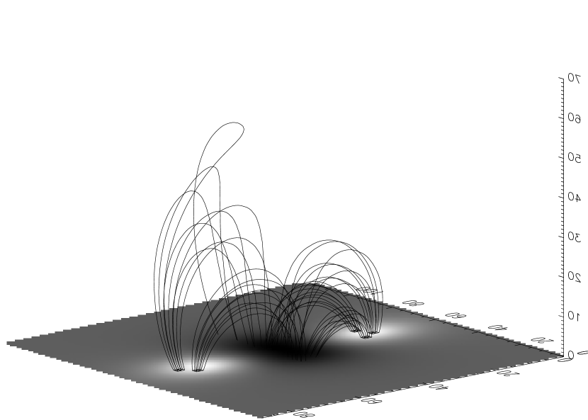
A volume of synthetic coronal emission was prepared as a test target for the SMART algorithm. The test target is more complex than any that have proven tractable for previous approaches to tomographic analysis for STEREO. It is not an attempt at detailed atmospheric modeling, but resembles a small active region. I began with a potential field defined by four sub-photospheric magnetic charges. The resulting line-of-sight photospheric magnetic field is shown in figure 1. The field lines in the figure emerge from five small, square “heated” patches in the postive polarities on the photospheric plane. A large number of field linese were traced from random points in the volume to both footpoints (or to the boundary). Emission was added to each voxel crossed by the field line, in proportion to the arbitrary heating value at its positive photospheric footpoint. Figure 2 shows the volume model projected along each of the three axes of figure 1. The coronal flux tubes have complicated geometries, including a broad, vertical fan of emission above the postive pole that is associated with a coronal magnetic null at a height of $\sim 53$ grid points. All images of EUV emission in this letter are square-root scaled to bring out faint features.

Figure 1.— Vertical magnetic field (shaded plane) and field lines within the emission from the model corona. five “Heated” patches within the positive photospheric magnetic poles are colored in black. Note the sharp deflection of the upppermost field line from the coronal null.

Figure 2.— The model coronal volume viewed along each of the three axes of figure 1. Intensities are square-root scaled.

Figure 3.— Synthetic data taken from three virtual spacecraft. Intensities are square-root scaled.

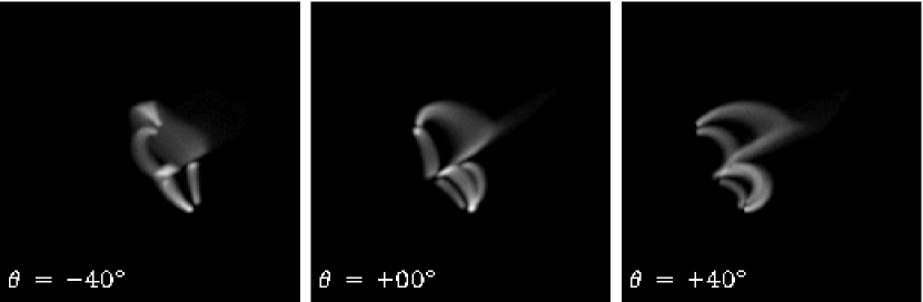
SMART was tested on numerous synthetic observations of the model coronal volume, each time placing the model active region at a different random northern heliographic latitude over $[0^{\circ},30^{\circ}]$, a random heliographic longitude over $[-40^{\circ},40^{\circ}]$, and a random tilt over the interval $[-180^{\circ},180^{\circ}]$. For simplicity, in our coordinate system the solar equator coincides with the equatorial plane. Observations were projected for three distant virtual instruments in the ecliptic, observing from heliographic longitudes $-40^{\circ},0^{\circ}$, and $40^{\circ}$. The twin STEREO spacecraft will reach similar separation angles in October, 2008. The images were normalized so that the brightest pixel among the three images had 3000 counts. The $\theta=(-40^{\circ},0^{\circ},40^{\circ})$ projections shown in figure 3 correspond to an example observation with the region placed at latitude $16.51^{\circ}$ N, longitude $14.65^{\circ}$ W, and tilt $29.63^{\circ}$ counter-clockwise. Poisson noise was applied to the images prior to passing them to the SMART algorithm for inversion. Intensities are square-root scaled to show the noise more clearly. The mean value of the nonzero pixels is 216 counts.

4. Inversion Results

The synthetic data were inverted using 15 SMART iterations. This was typically sufficient to converge to $\chi^{2}_{Rm}=1\pm 0.01$. The rate of convergence is affected by the smoothing parameter and by the two adjustable parameters in the control law. The examples shown in this Letter used $s=0.5$, $a=0.05$, $b=0.16$. Within broad limits, the results are insensitive to these parameters. For example, if the smoothing is removed altogether, numerical instabilities arise; if it is made too strong, then it will not be possible to reach $\chi^{2}_{Rm}=1$. For our computational volume of $169^{3}$ voxels, an inversion runs in a few minutes on a laptop computer.

Figure 4.— Comparison of true and reconstructed coronal volumes from three orthogonal points of view. Intensities are square-root scaled.

Figure 5.— Same as figure 4, but with loops nearly parallel to the ecliptic.

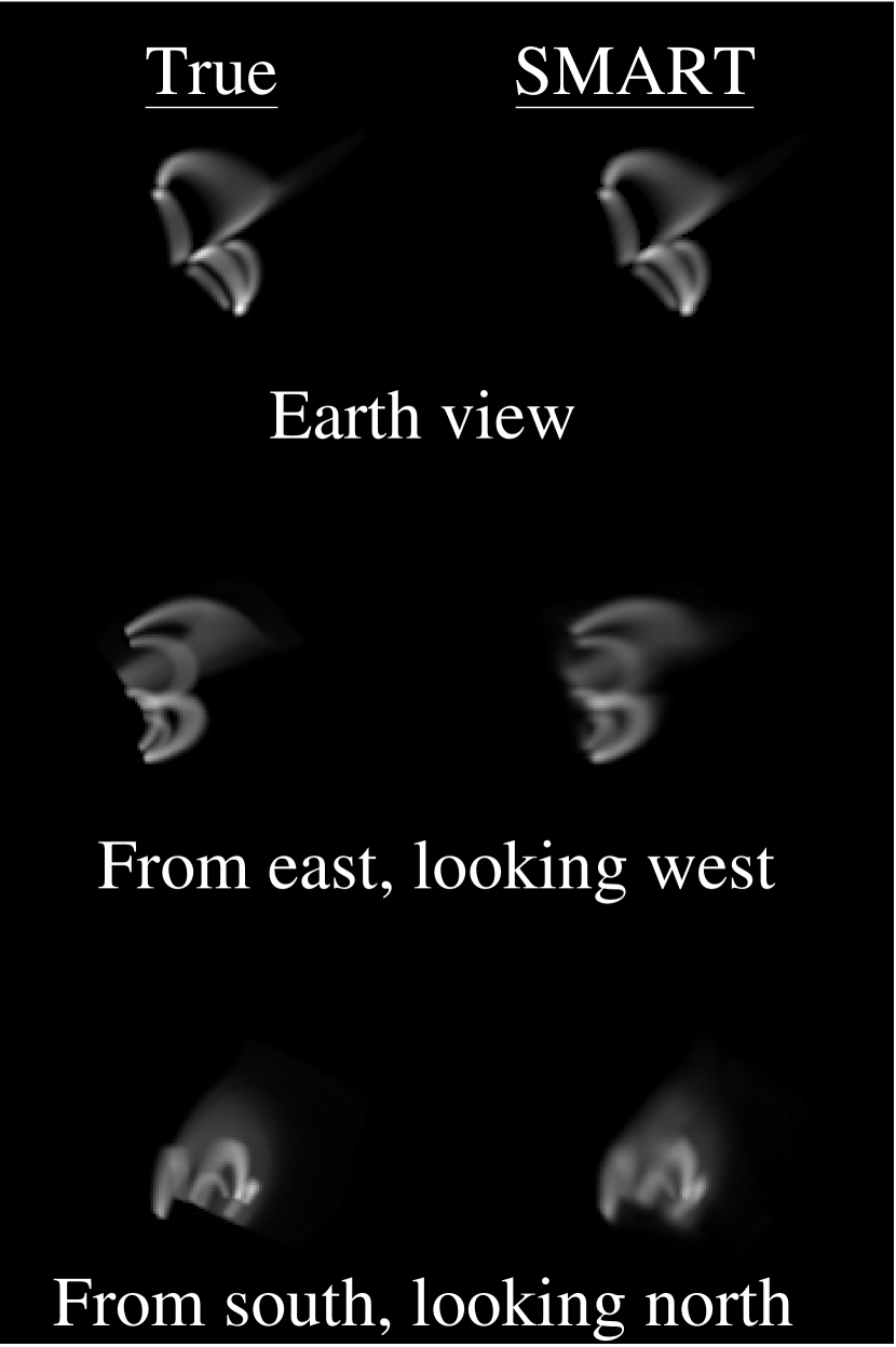
The simulated data in figure 3 gives rise to an accurate reconstruction.

Figure 4 shows reconstruction results for the data in figure 3, compared to noise-free visualizations of the coronal volume model. The Earth viewpoint at the top of figure 4 corresponds to the middle panel of figure 3. Comparing these two figures shows that the photon noise has been largely suppressed in the SMART reconstruction. The success at recovering 3D geometry is best illustrated by the east-west and south-north projections, which are $50^{\circ}$ and $90^{\circ}$, respectively, from the nearest available observing angles in the synthetic data. All of the true features have been recovered. Square-root scaling helps to bring out the artifacts, which are few and faint. There is slight blurring, and minimal ghosting. These results are typical of hundreds of realizations tried so far.

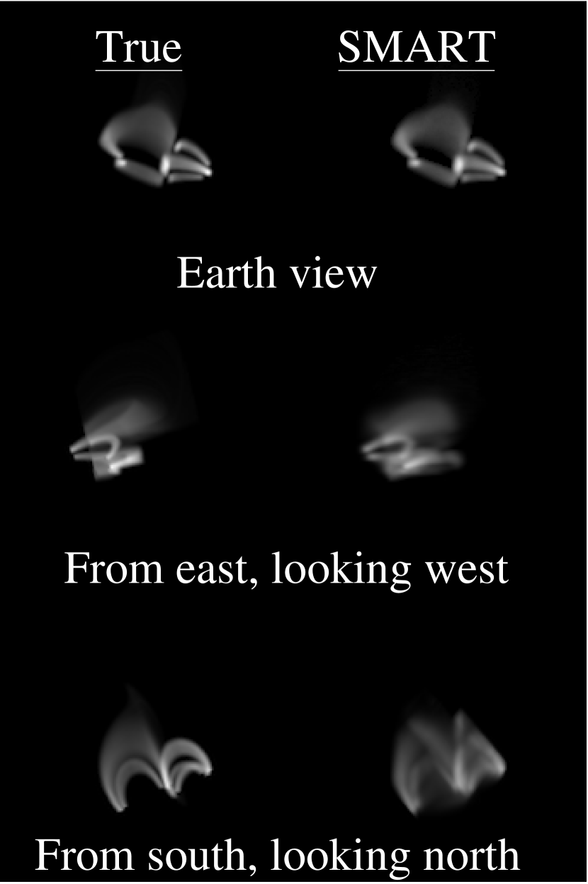
A second example, with loops nearly parallel to the ecliptic plane, is given in figure 5. The horizontal loop orientation is very challenging because only the ends of horizontal features provide any depth cues. Altough views from within the ecliptic plane are reproduced well, the example shows relatively poor reconstruction of an out-of-ecliptic view (lower panel). Animated versions of figures 4 and 5 are provided in the electronic version of the Journal.

5. Discussion and Conclusions

Coronal tomography is possible with as few as three viewpoints, making no prior assumptions about coronal morphology or magnetic fields. The test cases demonstrate recovery of complex geometry without reference to magnetic field extrapolations or assumptions about loop geometry. Loops that run in an east-west direction, however, provide insufficient depth cues for three instruments confined to the ecliptic.

The SMART algorithm described here provides a noise-insensitive tomographic reconstruction by finding an optimal balance between goodness of fit and local smoothness. STEREO will obtain data at large separation angles in Fall 2008. Observations from SOHO and/or TRACE at that time should allow the best opportunity for application of SMART to coronal tomography.

References

- Aschwanden (2005) Aschwanden, M. J. 2005, Sol. Phys., 228, 339
- Aschwanden et al. (2008) Aschwanden, M. J., Wülser, J.-P., Nitta, N. V., & Lemen, J. R. 2008, ApJ, 679, 827
- Fox et al. (2003) Fox, J. L., Kankelborg, C. C., & Metcalf, T. R. 2003, in Optical Spectroscopic Techniques and Instrumentation for Atmospheric and Space Research V., Larar, Allen M.; Shaw, Joseph A.; Sun, Zhaobo., eds. Proc. SPIE, Vol. 5157, 124–132
- Gary et al. (1998) Gary, G. A., Davis, J. M., & Moore, R. 1998, Sol. Phys., 183, 45
- Kankelborg & Thomas (2001) Kankelborg, C. C. & Thomas, R. J. 2001, in Visible Space Instrumentation for Astronomy and Solar Physics, Oswald H. Siegmund; Silvano Fineschi; Mark A. Gummin; Eds., Proc. SPIE, Vol. 4498, 16–26
- Okamoto & Yamaguchi (1991) Okamoto, T. & Yamaguchi, I. 1991, Optics Letters, 16, 1277
- Verhoeven (1993) Verhoeven, D. 1993, Applied Optics, 32, 3736
- Wiegelmann & Inhester (2006) Wiegelmann, T. & Inhester, B. 2006, Sol. Phys., 236, 25
- Wuelser et al. (2004) Wuelser, J.-P., Lemen, J. R., Tarbell, T. D., Wolfson, C. J., Cannon, J. C., Carpenter, B. A., Duncan, D. W., Gradwohl, G. S., Meyer, S. B., Moore, A. S., Navarro, R. L., Pearson, J. D., Rossi, G. R., Springer, L. A., Howard, R. A., Moses, J. D., Newmark, J. S., Delaboudiniere, J.-P., Artzner, G. E., Auchere, F., Bougnet, M., Bouyries, P., Bridou, F., Clotaire, J.-Y., Colas, G., Delmotte, F., Jerome, A., Lamare, M., Mercier, R., Mullot, M., Ravet, M.-F., Song, X., Bothmer, V., & Deutsch, W. 2004, in Telescopes and Instrumentation for Solar Astrophysics, Proc. SPIE, ed. S. Fineschi & M. A. Gummin, Vol. 5171, 111–122