A new Hedging algorithm and its application to inferring latent random variables

Abstract

We present a new online learning algorithm for cumulative discounted gain. This learning algorithm does not use exponential weights on the experts. Instead, it uses a weighting scheme that depends on the regret of the master algorithm relative to the experts. In particular, experts whose discounted cumulative gain is smaller (worse) than that of the master algorithm receive zero weight. We also sketch how a regret-based algorithm can be used as an alternative to Bayesian averaging in the context of inferring latent random variables.

1 Introduction

We study a variation on the online allocation problem presented by Freund and Schapire in [FS97]. Our problem varies from the original in that we use discounted cumulative loss instead of regular cumulative loss. Specifically, we consider the following iterative game between a hedger and Nature.

In this setting, there are $N$ actions (e.g. strategies, experts) indexed by $i$. The game between the hedger and Nature proceeds in iterations $j=0,1,2,\ldots$. In the $j$th iteration:

1. The hedger chooses a distribution $\{p_{i}^{j}\}_{i=1}^{N}$ over the actions, where $p_{i}^{j}\geq 0$ and $\sum_{i=1}^{N}p_{i}^{j}=1$.

2. Nature associates a gain $g_{i}^{j}\in[-1,1]$ with action $i$.

3. The gain of the hedger is $g^{j}_{A}=\sum_{i=1}^{N}p_{i}^{j}g_{i}^{j}$.

We define the discounted total gain as follows. The initial total gain is zero $G_{i}^{0}=0$. The total gain for action $i$ at the start of iteration $j+1$ is defined inductively as:

$$G_{i}^{j+1}\doteq(1-\alpha)G_{i}^{j}+g_{i}^{j}$$

for some fixed discount factor $\alpha>0$. The discounted total loss of the hedger is similarly defined:

$$G_{A}^{0}=0,\quad G_{A}^{j+1}\doteq(1-\alpha)G_{A}^{j}+g_{A}^{j}~{}.$$

We define the regret of the hedger with respect to action $i$ at the start of iteration $j$ as

$$R_{i}^{j}\doteq G_{i}^{j}-G_{A}^{j}$$

It is easy to see that the regret obeys the following recursion:

$$R_{i}^{0}=0,\quad R_{i}^{j+1}=(1-\alpha)R_{i}^{j}+g_{i}^{j}-g_{A}^{j}~{}.$$

Our goal is to find a hedging algorithm for which we can show a small uniform upper bound on the regret, i.e. a small positive real number $B(\alpha)$ such that $R_{i}^{j}\leq B(\alpha)$ for all choices of Nature, all $i$ and all $j$.

Our new hedging algorithm, which we call NormalHedge, uses the following weighting:

$$w_{i}^{j}\doteq\begin{cases}R_{i}^{j}\exp\left({\frac{\alpha\left[{R_{i}^{j}}\right]^{2}}{8}}\right)&\text{if $R_{i}^{j}>0$}\\ 0&\text{if $R_{i}^{j}\leq 0$.}\end{cases}$$ (1)

The hedging distribution is equal to the normalized weights $p_{i}^{j}=w_{i}^{j}/\sum_{k=1}^{N}w_{k}^{j}$ unless all of the weights are zero, in which case we use the uniform distribution $p_{i}^{j}=1/N$.

Our main result is that if $\alpha$ is sufficiently small, the following inequality holds uniformly over all game histories:

$${1\over N}\sum_{i=1}^{N}\Phi\left({\sqrt{\alpha}R_{i}^{j}}\right)<2.32$$

where

$$\Phi\left({x}\right)=\begin{cases}\exp\left({\frac{x^{2}}{8}}\right)&\text{if $x>0$}\\ 1&\text{if $x\leq 0$.}\end{cases}$$

This implies, in particular, that for any $i$ and $j$,

$$R_{i}^{j}\leq\sqrt{\frac{8\ln 2.32N}{\alpha}}.$$

The discount factor $\alpha$ plays a similar role to the number of iterations in the standard undiscounted cumulative loss framework. Indeed, it is easy to transform the usual exponential weights algorithms from the standard framework (e.g. Hedge [FS97]) to our present setting (Section 3). Such algorithms also enjoy discounted cumulative regret bounds of

$$R_{i}^{j}\leq C\cdot\sqrt{\frac{\ln N}{\alpha}}$$

for some positive constant $C$, but they require knowledge of the number of actions $N$ to tune a learning parameter. The tuning of NormalHedge does not have this requirement.

The rest of this paper is organized as follows. In Section 2 we describe the main ideas behind the construction and analysis of NormalHedge. In Sections 3 and 4 we discuss related work and compare NormalHedge to exponential weights algorithms. Finally, in Section 5 we suggest how to use NormalHedge to track latent variables and sketch how that might be used for learning HMMs under the $L_{1}$ loss.

2 NormalHedge

2.1 Preliminaries

NormalHedge and its analysis are based on the potential function $\Phi(x)$ introduced in Section 1. Here we give a slightly more elaborate definition for $\Phi(x)$ that includes a constant $c$. The potential function is a non-decreasing function of $x\in{\mathbb{R}}$

$$\Phi(x)\doteq\begin{cases}e^{x^{2}/2c}&\text{if $x>0$}\\ 1&\text{if $x\leq 0$}\end{cases}$$ (2)

where $c>1$. In our current version of NormalHedge, $c=4$. Decreasing $c$ will improve the bound on the regret; we will also argue that $c$ cannot be decreased to $1$.

The weights assigned by NormalHedge are set proportional to the first derivative of $\Phi$, i.e. $w_{i}^{j}=\Phi^{\prime}(R_{i}^{j})$, where

$$\Phi^{\prime}(x)=\begin{cases}{x\over c}e^{x^{2}/2c}&\text{if $x>0$}\\ 0&\text{if $x\leq 0$.}\end{cases}$$

In our analysis, we will also need to examine the second derivative of $\Phi$:

$$\Phi^{\prime\prime}(x)=\begin{cases}\left({{1\over c}+{x^{2}\over c^{2}}}\right)e^{x^{2}/2c}&\text{if $x>0$}\\ 0&\text{if $x<0$.}\end{cases}$$

Note that $\Phi^{\prime\prime}(x)$ has a discontinuity at $x=0$.

2.2 An intuitive derivation

The intuition behind the potential function is based on considering the following strategy for Nature. Suppose there are two types of actions, good actions and poor actions. The gain for each action on each iteration is chosen independently at random from a distribution over $\{-1,+1\}$. The distribution for poor actions has equal probabilities $1/2,1/2$ on the two outcomes, while the distribution for the good experts is $(1+\gamma)/2$ on $+1$ and $(1-\gamma)/2$ on $-1$ for some very small $\gamma>0$. Clearly, the best hedging strategy is to put equal positive weights on the good actions and zero weight on the poor actions. Unfortunately, the hedging algorithm does not know at the beginning of the game which experts are good, so it has to learn these weights online. Assuming that the number of actions is infinite (or sufficiently large), the per-iteration gain of the optimal weighting is $\gamma$, which implies that the discounted cumulative gain of this strategy is $\gamma/\alpha$.

Consider the regrets of this optimal hedging with respect to the good actions. It is not hard to show that the expected value of the discounted cumulative gain of a good action is $\gamma/\alpha$ and that the variance is approximately $1/\alpha$ (becomes exact as $\gamma\to 0$). Moreover, if $\alpha\to 0$ this distribution approaches a normal distribution with mean $\gamma/\alpha$ and variance $1/\alpha$. In other words, the distribution of the regrets of optimal hedging with respect to the good actions is $(1/Z)\exp(-\alpha R^{2}/2)$.

Consider the expected value of the potential function $\Phi(\sqrt{\alpha}R)$ for this distribution over the regrets. If we set $c=1$ we find that the product of the probability of the regret $R$ and the potential for the regret $R$ is a constant independent of $R$:

$$\frac{1}{Z}\cdot\exp\left(-\frac{\alpha R^{2}}{2}\right)\cdot\exp\left(\frac{\alpha R^{2}}{2}\right)=\frac{1}{Z}=\Omega(1).$$

Thus the expected potential is infinite. However, if we set $c$ to be larger than $1$ then the expected value of the potential function becomes finite. Thus, roughly speaking, the potential associated with a regret value is the reciprocal of the probability of that regret value being a result of random fluctuations. This level of regret is unavoidable. The design of NormalHedge is based on the goal of not allowing the average regret to grow beyond this level that is generated by random fluctuations. Ideally, we would be able to use a potential function with any constant $c$ larger than 1. However, what we are able to prove is that the algorithm works for $c=4$.

The idea of NormalHedge is to keep the average potential small. It is therefore natural that the weight assigned to each action is proportional to the derivative of the potential. Indeed, it is easily checked that the weights $w_{i}^{j}$ defined in Equation (1) are proportional to $\Phi^{\prime}(\sqrt{\alpha}R_{i}^{j})$. This derivative, however, is best viewed when the hedging game is mapped into continuous time.

2.3 The continuous time limit

Our analysis of NormalHedge is based on mapping the integer time steps $j=0,1,2,\ldots$ into real-valued time steps $t=0,\alpha,2\alpha,\ldots$ and then taking the limit $\alpha\to 0$. Formally, we redefine the hedging game using a different notation which uses the real valued time $t$ instead of the time index $j$. We assume a set of $N$ actions (experts), indexed by $i$. The game between the hedging algorithm and Nature proceeds in iterations $t=0,\alpha,2\alpha,\ldots$. At each iteration the following sequence of actions take place.

1. The hedging algorithm defines a distribution $\left\{{p_{i}\left({t}\right)}\right\}_{i=1}^{N}$ over the actions. $p_{i}\left({t}\right)\geq 0;\;\;\sum_{i=1}^{N}p_{i}\left({t}\right)=1$.

2. Nature associates a gain $g_{i}\left({t}\right)\in[-\sqrt{\alpha},+\sqrt{\alpha}]$ with action $i$.

3. The gain of the hedger is $g_{A}\left({t}\right)=\sum_{i=1}^{N}p_{i}\left({t}\right)g_{i}\left({t}\right)$.

We skip the definitions of $G_{i}(t)$ and $G_{A}(t)$ as these can become ill-behaved when $\alpha\to 0$. Instead we define the regret directly:

$$R_{i}\left({0}\right)=0,\;\;R_{i}\left({t+\alpha}\right)=(1-\alpha)R_{i}\left({t}\right)+g_{i}\left({t}\right)-g_{A}\left({t}\right)~{}.$$

Note that this definition of the regret is a scaled version of the discrete time regret:

$$R_{i}\left({j\alpha}\right)=\sqrt{\alpha}R_{i}^{j}.$$

We now have the tools needed to prove our main result.

Theorem 1

There exists a positive constant $C<2.32$ such that if $\alpha<1/(800\ln CN)$, then for any sequence of gains and any iteration $j$

$$\frac{1}{N}\sum_{i=1}^{N}\Phi\left({\sqrt{\alpha}R_{i}^{j}}\right)<C.$$

Proof sketch. The full proof is given in the appendix, but here we sketch a continuous-time argument (i.e. we consider $\alpha\to 0$). The formal, discrete-time proof shows that it is enough for $\alpha\leq 1/(800\ln CN)$.

We want to show that the average potential

$$\Psi(t)\doteq\frac{1}{N}\sum_{i=1}^{N}\Phi(t)$$

is bounded for all time $t$. Our approach is to show that its time-derivative

$$\frac{\partial}{\partial t}\Psi(t)=\lim_{\alpha\to 0}\frac{1}{\alpha}\cdot\frac{1}{N}\sum_{i=1}^{N}\left\{\Phi(R_{i}\left({t+\alpha}\right))-\Phi(R_{i}\left({t}\right))\right\}$$

becomes non-positive as soon as $\Psi(t)$ is above some constant (recall that the time steps are in increments of $\alpha$). Since the $\Phi(x)$ is constant for $x<0$, we need only consider $i$ such that $R_{i}\left({t+\alpha}\right)\geq 0$. Ignoring the discontinuity of $\Phi^{\prime\prime}(x)$ at $x=0$, Taylor’s theorem implies that for some $\rho_{i}\leq\max\{R_{i}\left({t}\right),R_{i}\left({t+\alpha}\right)\}$,

$$\sum_{i:R_{i}\left({t}\right)\geq 0}\Phi(R_{i}\left({t+\alpha}\right))-\Phi(R_{i}\left({t}\right)) = \sum_{i:R_{i}\left({t}\right)\geq 0}\Phi((1-\alpha)R_{i}\left({t}\right)+g_{i}(t)-g_{A}(t))-\Phi(R_{i}\left({t}\right))$$

$$= \sum_{i:R_{i}\left({t}\right)\geq 0}(-\alpha R_{i}\left({t}\right)+g_{i}(t)-g_{A}(t))\Phi^{\prime}(R_{i}\left({t}\right))$$

$$\quad\quad\quad\mbox{}+\frac{1}{2}(g_{i}(t)-g_{A}(t)-\alpha R_{i}\left({t}\right))^{2}\Phi^{\prime\prime}(\rho_{i})$$

$$\leq \sum_{i:R_{i}\left({t}\right)\geq 0}-\alpha R_{i}\left({t}\right)\Phi^{\prime}(R_{i}\left({t}\right))+\frac{1}{2}(g_{i}(t)-g_{A}(t)-\alpha R_{i}\left({t}\right))^{2}\Phi^{\prime\prime}(\rho_{i})$$

$$\leq \sum_{i:R_{i}\left({t}\right)\geq 0}-\alpha R_{i}\left({t}\right)\Phi^{\prime}(R_{i}\left({t}\right))+\frac{1}{2}(2\sqrt{\alpha}+\alpha R_{i}\left({t}\right))^{2}\Phi^{\prime\prime}(R_{i}\left({t}\right)+2\sqrt{\alpha}).$$

The first inequality uses the fact that the weights are proportional to the derivatives of the potentials

$$\sum_{i:R_{i}\left({t}\right)\geq 0}g_{i}(t)\cdot\frac{\Phi^{\prime}(R_{i}\left({t}\right))}{\sum_{j:R_{j}\left({t}\right)\geq 0}\Phi^{\prime}(R_{j}\left({t}\right))}=g_{A}(t),$$

and the second inequality follows because $|g_{i}(t)-g_{A}(t)|\leq 2\sqrt{\alpha}$. Now dividing by $\alpha$ and $N$ and taking the limit $\alpha\to 0$, we have

$$\frac{\partial}{\partial t}\Psi(t) \leq \lim_{\alpha\to 0}\frac{1}{\alpha}\cdot\frac{1}{N}\sum_{i:R_{i}\left({t}\right)\geq 0}\frac{1}{2}(2\sqrt{\alpha}+\alpha R_{i}\left({t}\right))^{2}\Phi^{\prime\prime}(R_{i}\left({t}\right)+2\sqrt{\alpha})-\alpha R_{i}\left({t}\right)\Phi^{\prime}(R_{i}\left({t}\right))$$

$$= \lim_{\alpha\to 0}\frac{1}{N}\sum_{i:R_{i}\left({t}\right)\geq 0}\frac{1}{2}(2+\sqrt{\alpha}R_{i}\left({t}\right))^{2}\Phi^{\prime\prime}(R_{i}\left({t}\right)+2\sqrt{\alpha})-R_{i}\left({t}\right)\Phi^{\prime}(R_{i}\left({t}\right))$$

$$= \frac{1}{N}\left\{2\left(\frac{1}{c}+\frac{R_{i}\left({t}\right)^{2}}{c^{2}}\right)\exp(R_{i}\left({t}\right)^{2}/2c)-\frac{R_{i}\left({t}\right)^{2}}{c}\exp(R_{i}\left({t}\right)^{2}/2c)\right\}$$

$$\leq \frac{2}{c}\Psi(t)+\frac{1}{cN}\sum_{i=1}^{N}\left(\frac{2}{c}-1\right)R_{i}\left({t}\right)^{2}\exp(R_{i}\left({t}\right)^{2}/2c).$$

If $\Psi(t)\geq B$, then this final RHS is maximized when $R_{i}(t)\equiv\sqrt{2c\ln B}$ for all $i$, whereupon

$$\frac{\partial}{\partial t}\Psi(t)\leq\frac{2B}{c}\left(1+\left(\frac{2}{c}-1\right)c\ln B\right).$$

This is non-positive for sufficiently large $B$ and $c\geq 2+1/\ln B$.  

3 Related work

3.1 Relation to other online learning algorithms

The Hedge algorithm [FS97], as well as most of the work on online learning algorithms is based on exponential weighting, where the weight assigned to an expert is exponential in the cumulative loss of that expert. NormalHedge uses a very different weighting scheme. The most important difference is that the weight of an expert depends on the regret of the master algorithm relative to that expert, rather than just on the loss of the algorithm. In particular, experts whose discounted cumulative loss is larger than that of the master algorithm receive zero weight. We expand on the comparison of NormalHedge to Hedge in Section 4.

The starting point for the derivation and analysis of NormalHedge is the Binomial Weights algorithm of Cesa-Bianchi et al [CBFHW96]. The Binomial weights algorithm is an algorithm for a restricted version of the experts prediction problem [LW94, CBFH⁺97]. In this version sequence to be predicted is binary and all of the predictions are also binary. The Binomial Weights algorithm is analyzed using a type of chip game. In this game each expert is represented as a chip, at each iteration each chip has a location on the integer line. The position of the chip corresponds to the number of mistakes that were made by the expert. The a-priori assumption is that there is at least one experts which makes at most $k$ mistakes, and the goal is to define a rule for combining the experts predictions in a way that would minimize the maximal number of mistakes of the master expert.

The chip game analysis leads naturally to the definition of the potential function and the evolution of this potential function from iteration to iteration yields the Binomial Weights algorithm. A closely related notion of potential was used in the Boost-by-Majority algorithm. The chip-game analysis was extended by Schapire’s work on drifting games [Sch01] and by Freund and Opper’s work on drifting games in continuous time [FO02]. NormalHedge naturally extends the continuous time drifting games to a setting in which one seeks to minimize discounted loss.

3.2 Relation to switching and sleeping experts

The use of discounted cumulative loss represents an alternative to the “switching experts” framework of Warmuth and Herbster [HW98]. If the best expert changes at a rate of $O(\alpha)$, then NormalHedge will switch to the new best expert because the losses that occurred more than $1/\alpha$ iterations ago make a small contribution to the discounted total loss.

A useful extension of NormalHedge is to using experts that can abstain, similar to the setup studied in  [FSSW97]. To do this we assume that each expert $i$, at each iteration $j$, outputs a confidence level $0\leq c\leq 1$. Instead of using the vector $\{p_{i}^{j}\}_{j=1}^{N}$ the hedger uses the vector $\{p_{i}^{j}c_{i}^{j}/Z^{j}\}_{j=1}^{N}$ where $Z=\sum_{i=1}^{N}p_{i}^{j}c_{i}^{j}$. The gain $g_{i}^{j}$ of action $i$ at iteration $j$ is replaced by $c_{i}^{j}g_{i}^{j}$, and the discounted cumulative gain and the discounted cumulative regret change in the corresponding way. The bounds on the average potential transfer without change. This allows an expert to abstain from making a prediction. By setting $c_{i}^{j}=0$ the expert effectively removes itself from the pool of experts used by the hedger. It also avoids suffering any loss. However, an expert cannot always abstain, because then it’s discounted cumulative gain will be driven to zero by the discount factor. We will use this extension in Section 5.

4 Comparison of NormalHedge and Hedge

4.1 Discounted regret bound for Hedge

To ease the comparison, we first recast the Hedge algorithm [FS97] into our current framework with discounted gains. The weights used by Hedge are

$$w_{i}^{j}\doteq\exp(\eta G_{i}^{j})$$

where $G_{i}^{j}$ is the discounted cumulative gain of action $i$ at the start of iteration $j$, and $\eta>0$ is the learning rate parameter. When written recursively as

$$w_{i}^{j+1}=\exp\left(\eta((1-\alpha)G_{i}^{j}+g_{i}^{j})\right)\propto\left(w_{i}^{j}\right)^{1-\alpha}\exp(\eta g_{i}^{j}),$$

we see that the effect of discounting is a dampening of the previous weights $w_{i}^{j}$ prior to the usual multiplicative update rule.

Fix any iteration $j$ and define the adjusted cumulative gain of action $i$ at the start of iteration $k$ to be

$$\widehat{G}_{i}^{k}=\sum_{s=1}^{k-1}(1-\alpha)^{j-1-s}g_{i}^{s}$$

with $G_{i}^{0}=0$. The gain of Hedge in iteration $k$ is

$$g_{A}^{k}=\frac{\sum_{i=1}^{N}w_{i}^{k}g_{i}^{k}}{\sum_{i=1}^{N}w_{i}^{k}}=\frac{\sum_{i=1}^{N}e^{\eta\widehat{G}_{i}^{k}}g_{i}^{k}}{\sum_{i=1}^{N}e^{\eta\widehat{G}_{i}^{k}}}$$

and the adjusted cumulative gain of Hedge at the start of iteration $k$ is

$$\widehat{G}_{A}^{k}=\sum_{s=1}^{k-1}(1-\alpha)^{j-1-s}g_{A}^{s}.$$

Then the discounted cumulative regret to action $i$ at the start of iteration $j$ is $\widehat{G}_{i}^{j}-\widehat{G}_{A}^{j}$.

We analyze the (log of the) ratios $W_{k}/W_{k-1}$, where

$$W_{k}=\sum_{i=1}^{N}e^{\eta\widehat{G}_{i}^{k}}$$

and $W_{0}=N$. We lower bound $\ln(W_{j}/W_{0})$ as

$$\ln\frac{W_{j}}{W_{0}}=\ln\sum_{i=1}^{N}e^{\eta\widehat{G}_{i}^{j}}-\ln N\geq\ln e^{\eta\widehat{G}_{i}^{j}}-\ln N=\eta\widehat{G}_{i}^{j}-\ln N$$

(for any $i$), and we upper bound it as

$$\ln\frac{W_{j}}{W_{0}} =\sum_{k=1}^{j-1}\ln\frac{W_{j}}{W_{j-1}}$$

$$=\sum_{k=1}^{j-1}\ln\frac{\sum_{i=1}^{N}e^{\eta\widehat{G}_{i}^{k-1}}e^{\eta(1-\alpha)^{j-1-k}g_{i}^{k}}}{\sum_{i=1}^{N}e^{\eta\widehat{G}_{i}^{k-1}}}$$

$$\leq\sum_{t=1}^{T}\eta\cdot\frac{\sum_{i=1}^{N}e^{\eta\widehat{G}_{i}^{k-1}}(1-\alpha)^{j-1-k}g_{i}^{k}}{\sum_{i=1}^{N}e^{\eta G_{i}^{k-1}}}+\frac{\eta^{2}}{8}\cdot 4(1-\alpha^{2(j-1-k)}\quad\text{(Hoeffding's inequality)}$$

$$=\sum_{k=1}^{j-1}\eta(1-\alpha)^{j-1-k}g_{A}^{k}+\frac{\eta^{2}}{2}(1-\alpha)^{2(j-1-k)}$$

$$=\eta\widehat{G}_{A}^{k}+\frac{\eta^{2}}{2}\cdot\frac{1}{1-(1-\alpha)^{2}}$$

$$=\eta\widehat{G}_{A}^{k}+\frac{\eta^{2}}{4(\alpha-\alpha^{2}/2)}.$$

Therefore, the discounted cumulative regret of Hedge to action $i$ at the start of any iteration $j$ is

$$R_{i}^{j}=\widehat{G}_{i}^{j}-\widehat{G}_{A}^{j}\leq\frac{\ln N}{\eta}+\frac{\eta}{4(\alpha-\alpha^{2}/2)}.$$

Choosing $\eta=\sqrt{4(\alpha-\alpha^{2}/2)\ln N}$ gives

$$R_{i}^{j}\leq\sqrt{\frac{\ln N}{\alpha-\alpha^{2}/2}}.$$

The regret bound is of the same form as that implied by Theorem 1, indeed, with better leading constants. However, this bound only holds when $\eta$ is tuned with knowledge of the number of actions $N$. If instead one sets $\eta=\Theta(\sqrt{\alpha})$ independently of $N$, the bound for Hedge is worse by a factor of $\Theta(\sqrt{\ln N})$. Furthermore, this setting of $\eta$ is for optimizing a bound that anticipates the worst-case sequence of gains; when Nature is not optimally adversarial, then a proper setting of $\eta$ may require other prior knowledge.

4.2 Simulations

4.2.1 The effect of good experts

To empirically compare Hedge and NormalHedge, we first simulated the two algorithms in a scenario similar to that described in Section 2:

• The number of experts is $N=1000$, and the discount parameter is $\alpha=0.001$.

• At any given time, there is a set of $N_{G}=f\cdot N$ good experts and $N-N_{G}$ bad experts. (We varied $f\in\{0.001,0.01,0.1,0.5\}$.)

  • With probability $0.5+\gamma/2$, every good expert receives gain $+1$; with probability $0.5-\gamma/2$, every good expert receives gain $-1$. (We varied $\gamma\in\{0.2,0.4,0.6,0.8\}$.)

  • Bad experts receive gain $+1$ and $-1$ with equal probability.

• Initially, the set of good experts is $\{0,1,\ldots,N_{G}-1\}$.

• After every $1/\alpha$ iterations, the set of good experts shifts from $\{i_{0},i_{0}+1,\ldots,i_{0}+N_{G}-1\}$ to $\{i_{0}+N_{G},i_{0}+N_{G}+1,\ldots,i_{0}+2N_{G}-1\}$ (with addition modulo $N$).

Thus, the set of good experts completely changes every $1/\alpha$ iterations. In each iteration, all good experts receive the same gain, which is $\gamma$ in expectation. In contrast, the gain of each bad expert is decided independently with a fair coin.

We tuned the learning rate parameter for Hedge to $\eta=\sqrt{(\alpha-\alpha^{2}/2)\ln N}$. For NormalHedge, we varied $c\in\{1,2,4\}$. Recall that the regret bound we can show for NormalHedge holds for $c=2$ as $\alpha\to 0$ (the formal proof is stated with $c=4$).

Figures 1 and 2 depict the discounted cumulative regret to the best expert (averaged over $50$ runs). First, we observe that NormalHedge fares better than Hedge when the advantage of the good experts is large and the fraction of experts that are good is large. In such cases, the advantage of NormalHedge is especially pronounced within $1/\alpha$ iterations (before the set of good experts shifts). Second, we observe that the performance of NormalHedge generally improves as the value of $c$ is decreased. Indeed, the setting of $c=1$ (for which we have no theoretical guarantees) yields the best results for NormalHedge (and in fact outperforms Hedge in every simulation). It would be very interesting to establish guarantees for NormalHedge for $c\to 1$.

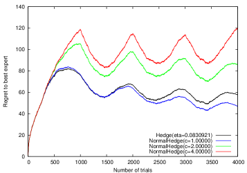
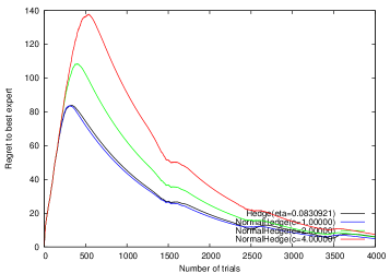
$\gamma=0.2,f=0.001$	$\gamma=0.4,f=0.001$
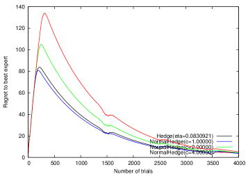
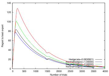
$\gamma=0.6,f=0.001$	$\gamma=0.8,f=0.001$
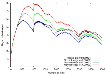
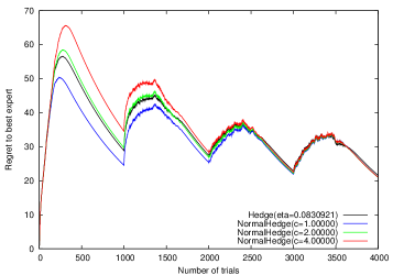
$\gamma=0.2,f=0.01$	$\gamma=0.4,f=0.01$
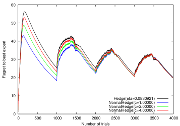
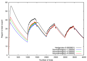
$\gamma=0.6,f=0.01$	$\gamma=0.8,f=0.01$

Figure 1: Regrets to the best expert in the first simulation; $\gamma\in\{0.2,0.4,0.6,0.8\}$ and $f\in\{0.001,0.01\}$.

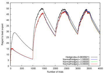
$\gamma=0.2,f=0.1$	$\gamma=0.4,f=0.1$
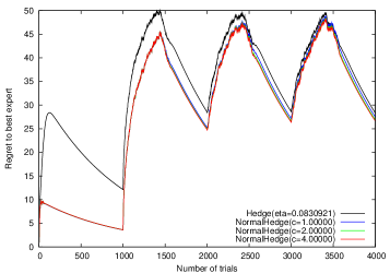
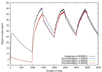
$\gamma=0.6,f=0.1$	$\gamma=0.8,f=0.1$
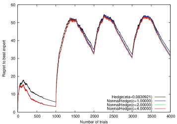
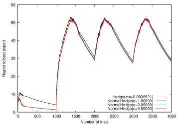
$\gamma=0.2,f=0.5$	$\gamma=0.4,f=0.5$
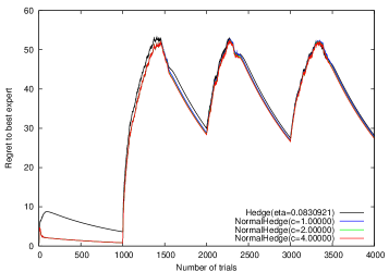
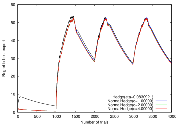
$\gamma=0.6,f=0.5$	$\gamma=0.8,f=0.5$

Figure 2: Regrets to the best expert in the first simulation; $\gamma\in\{0.2,0.4,0.6,0.8\}$ and $f\in\{0.1,0.5\}$.

4.2.2 The effect of tuning $\eta$ in Hedge

Next, to bring out the issue with parameter tuning in Hedge, we conducted a simulation in which we fix the fraction of experts that are good, but vary the total number of experts:

• The number of experts is $N$, and the discount parameter is $\alpha=0.001$. (We varied $N\in\{10,100,1000\}$.)

• The fraction of experts that are good is fixed at $f=0.1$. The notion of good and bad experts is the same as in the first simulation. (We varied $\gamma\in\{0.2,0.8\}$.)

• The remaining details are the same as in the first simulation.

Again, we tuned the learning rate parameter for Hedge to $\eta=\sqrt{(\alpha-\alpha^{2}/2)\log N}$, which now changes as we vary the total number of experts, and we varied $c\in\{1,2,4\}$ in NormalHedge.

The results (Figure 3) indicate that as $N$ decreases (e.g. $N=100,10$), the disparity between Hedge and NormalHedge increases. We believe this is an issue with tuning the learning rate $\eta$, which is conspicuously absent in NormalHedge, but we have not precisely characterized the issue.

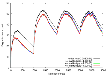
$\gamma=0.2,N=1000$	$\gamma=0.8,N=1000$
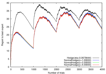
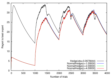
$\gamma=0.2,N=100$	$\gamma=0.8,N=100$
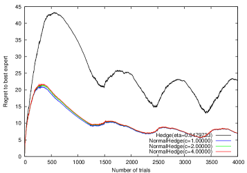
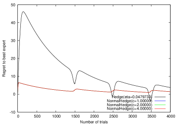
$\gamma=0.2,N=10$	$\gamma=0.8,N=10$

Figure 3: Regrets to the best expert in the second simulation; $\gamma\in\{0.2,0.8\}$ and $N\in\{1000,100,10\}$.

5 Inferring latent random variables

An important problem in statistical inference is to make predictions or choose actions when the system under consideration has internal states that cannot be observed directly. There are many manifestations of this problem, including Graphical models, Hidden Markov Models (HMMs), Partially Observable Markov Decision Processes (POMDPs) and Kalman filters. The common method for dealing with hidden states is to model them as latent random variables. The relation between the latent random variables and the observable random variables is modeled using a joint probability distribution. Two very important sub-problems that arise in this approach are learning joint distributions the involve latent random variables from examples that contain only the state of the observable random variables and using this type of joint distributions to infer the value of some variables given the state of others. At this time there is no good universal solution to either of these sub-problems.

We propose a different approach to the problem, where instead of associating hidden states with hidden random variables, we associate states with different experts. What we present here describes some initial ideas. It is not an attempt to propose a solution to this large and complex problem.

Suppose that we are to predict a binary sequence $x_{1},x_{2},\ldots$, $x_{t}\in\{0,1\}$ and suppose that we believe that the sequence can be predicted reasonably well using a Hidden Markov Model. Specifically, suppose there is a hidden state $S$ which attains one of the values $1,\ldots,k$ at each time step. Suppose that the state transition is Markovian and stationary, i.e.

$$P(S_{t}|S_{t-1},S_{t-2},\ldots)=P(S_{t}|S_{t-1})=P(S_{t-1}|S_{t-2})=\cdots$$

Assume in addition that the hidden state does not change very often, i.e. $P(S_{t+1}=S_{t})$ is close to 1. Finally, assume that the distribution of the observable variable $X_{t}$ depends only on the hidden state at the same time $S_{t}$.

Consider the problem of predicting $X_{t+1}$ given $x_{1},\ldots,x_{t}$ and the parameters of the HMM. Suppose that the prediction needs to take the form of a distribution over $\Sigma$. So far this is exactly the standard framework, but suppose we differ from the standard framework by considering the $L_{1}$ loss $1-p_{t}(x_{t})$, where $p_{t}(x_{t})$ is the predicted probability assigned to the letter that actually occured at time $t$. This is instead of the standard log likelihood loss $\log(1/p_{t}(x_{t})$. While the log loss is easier to analyze, the $L_{1}$ loss is often a more useful measure because the cumulative $L_{1}$ loss corresponds to the expected number of mistakes. While this loss does not fit well in the maximal likelihood or Bayesian methodologies, it fits NormalHedge very well, because the loss per-iteration is bounded.

Here is our proposal for solving the prediction problem using NormalHedge. We associate a set of experts with each hidden state. The experts are confidence rated, i.e. each one of the experts outputs a confidence level $0\leq c\leq 1$ at each time step, the confidence level is used in the confidence rated variant of NormalHedge described in the previous section. If expert $i$ corresponds to a hidden state $j$ then $c_{i}$ should be large when $S=j$ and low when $S\neq j$. Suppose that the parameters of the HMM are known, then we can associate a single expert with each hidden state and compute the prediction and the confidence value of that expert using Bayes formula.

Now suppose that we don’t know the parameter vector of the HMM but that we know that the vector is one of $N$ possibilities. In this case we associate $N$ experts with each hidden state and compute the predictions and confidence value of each expert using Bayes Formula for the corresponding parameter vector, the confidence value for each state is the a-posteriori probability for that state.

In this case the NormalHedge algorithm will quickly converge and give most of the weight to the experts that correspond to the correct parameter vector. Moreover, if none of the parameter vectors is a correct description of the sequence distribution, it will converge on the vector which causes the least regret, i.e. makes the smallest number of mistakes.

Contrast this with the Bayesian approach. If the true distribution generating the data is not included in the set of models over which we take the posterior average, and if the loss function in which we are interested is not log-likelihood but rather number of mistakes. Then the cumulative loss of the Bayesian average can be much larger than that of the best model in the set.

6 Open problems

The most interesting open problem is to close the gap between the upper bound and lower bound on the parameter $c$. We have a lower bound of $c>1$ and an upper bound of $c=4$. If we consider the case $\alpha\to 0$ we can reduce $c$ to $2$. However, the gap between $c=1$ and $c=2$ remains.

One promising direction of expansion is to consider the game in the continuous time limit directly. This leads us naturally into stochastic processes in continuous time such as Wiener processes. Understanding the performance of NormalHedge in this context might yield new methods for stochastic estimation and stochastic control.

Appendix A Proof of main theorem

Recall, the cumulative discounted regret of action $i$ at time $t=j\alpha$, $j\in{\mathbb{N}}$ is defined recursively by

$$R_{i}(0)=0,\quad R_{i}(t+\alpha)=(1-\alpha)R_{i}(t)+g_{i}(t)-g_{A}(t),$$

where $g_{i}(t)\in[-\sqrt{\alpha},+\sqrt{\alpha}]$ is the (scaled) gain of action $i$ at time $t$, and $g_{A}(t)\in[-\sqrt{\alpha},+\sqrt{\alpha}]$ is the (scaled) gain of the hedger at time $t$. We define $r_{i}(t)=(g_{i}(t)-g_{A}(t))/\sqrt{\alpha}\in[-2,+2]$ as the (unscaled) instantaenous regret to action $i$ at time $t$. The central quantity of interest is the average potential

$$\Psi(t)=\frac{1}{N}\sum_{i=1}^{N}\Phi(R_{i}(t)).$$

Recall, we use the definition of the potential function $\Phi$ in Equation (2) with $c=4$.

Claim 1

There exists a positive constant $C\leq 2.32$ such that if $\alpha<1/(800\ln CN)$, then the average potential is always bounded from above by $C$; that is, $\Psi(j\alpha)<C$ for any $j\in{\mathbb{N}}$.

Proof. Fix $j\in{\mathbb{N}}$ and let $t=j\alpha$.

We will analyze the average $\Psi(t+\alpha)-\Psi(t)$ by considering the averages over two separate groups:

$$I_{1}=\{i:R_{i}(t)\leq 0\}\quad\text{and}\quad I_{2}=\{i:R_{i}(t)>0\}.$$

Let $\Psi_{k}(t)=(1/|I_{k}|)\sum_{i\in I_{k}}\Phi(R_{i}(t))$ be the average potential for $I_{k}$, $k=1,2$ (assume without loss of generality that neither $I_{k}$ is empty). We’ll show the following facts:

1. $\Psi_{1}(t)=1$ and $\Psi_{1}(t+\alpha)<1+(3/5)\alpha$;

2. If $\Psi(t)<2.32$, then $\Psi_{2}(t+\alpha)-\Psi_{2}(t)<(2/3)\alpha$;

3. If $2.31<\Psi(t)<2.32$, then $\Psi(t+\alpha)<\Psi(t)$.

These facts imply that the increase in average potential from $\Psi(t)$ to $\Psi(t+\alpha)$ is always less than $(2/3)\alpha<1/1200$, and that if the average potential $\Psi(t)$ is strictly between $2.31$ and $2.32$, then $\Psi(t+\alpha)$ is strictly less than $\Psi(t)$. The claim then follows by induction because $\Psi(0)=1$.

We now prove the facts (A), (B), and (C).

(A): For $i\in I_{1}$, $\Phi(R_{i}(t))=1$ and $R_{i}(t+\alpha)\leq(1-\alpha)R_{i}(t)+|r_{i}(t)|\sqrt{\alpha}\leq 2\sqrt{\alpha}$. Since $\Phi(x)$ is non-decreasing in $x$, we have $\Phi(R_{i}(t+\alpha))\leq\Phi(2\sqrt{\alpha})=e^{\alpha/2}<1+\alpha/2+\alpha^{2}e^{\alpha/2}/2<1+(3/5)\alpha$ (the last inequality follows from the upper bound on $\alpha$).

(B): We address terms in $I_{2}$ by expanding $\Phi(R_{i}(t+\alpha))$ around the point $R_{i}(t)\neq 0$ via Taylor’s theorem:

$$\Phi(R_{i}(t+\alpha))=\Phi(R_{i}(t))+d_{i}(t)\Phi^{\prime}(R_{i}(t))+\frac{1}{2}d_{i}(t)^{2}\Phi^{\prime\prime}(\rho_{i})$$

where $d_{i}(t)=r_{i}(t)\sqrt{\alpha}-\alpha R_{i}(t)$ and $\rho_{i}\in{\mathbb{R}}$ lies between $R_{i}(t)$ and $R_{i}(t+\alpha)$. Because the hedger’s weights are chosen so that $p_{i}(t)\propto\Phi^{\prime}(R_{i}(t))$, we have that

$$\sum_{i=1}^{N}g_{i}(t)\Phi^{\prime}(R_{i}(t))-g_{A}(t)\sum_{i=1}^{N}\Phi^{\prime}(R_{i}(t))=0$$

and thus

$$\Phi(R_{i}(t+\alpha))-\Phi(R_{i}(t))=-\alpha R_{i}(t)\Phi^{\prime}(R_{i}(t))+\frac{1}{2}d_{i}(t)^{2}\Phi^{\prime\prime}(\rho_{i}).$$

We need a few bounds before proceeding. First, if $\Psi(t)<2.32$, then $\Phi(R_{i}(t))<2.32N$ for all $i$, which implies $R_{i}(t)<\sqrt{8\ln(2.32N)}$ for all $i$. By the condition on $\alpha$, we also have $\sqrt{\alpha}R_{i}(t)<1/10$. Next, we use a bound on $\rho_{i}$ since it is evaluated in the non-decreasing function $\Phi^{\prime\prime}(x)$:

$$\rho_{i}^{2}\ \leq\ \max\{R_{i}(t),R_{i}(t+\alpha)\}^{2}\ \leq\ (R_{i}(t)+|r_{i}(t)|\sqrt{\alpha})^{2}\ =\ R_{i}(t)^{2}+2\sqrt{\alpha}R_{i}(t)|r_{i}(t)|+\alpha r_{i}(t)^{2}\ \leq\ R_{i}(t)^{2}+\frac{1}{2}.$$

Finally, we bound $d_{i}(t)^{2}$ as follows:

$$d_{i}(t)^{2}\ \leq\ (|r_{i}(t)|\sqrt{\alpha}+\alpha R_{i}(t))^{2}\ \leq\ (2+1/10)^{2}\alpha\ \leq\ \frac{9}{2}\alpha.$$

Altogether, we have

$$\Phi(R_{i}(t+\alpha))-\Phi(R_{i}(t)) =-\alpha R_{i}(t)\Phi^{\prime}(R_{i}(t))+\frac{1}{2}d_{i}(t)^{2}\Phi^{\prime\prime}(\rho_{i})$$

$$=-\alpha R_{i}(t)\frac{R_{i}(t)}{4}e^{R_{i}(t)^{2}/8}+\frac{1}{2}d_{i}(t)^{2}\left(\frac{1}{4}+\frac{\rho_{i}^{2}}{16}\right)e^{\rho_{i}^{2}/8}$$

$$\leq-\alpha\frac{R_{i}(t)^{2}}{4}e^{R_{i}(t)^{2}/8}+\frac{9\alpha}{4}\left(\frac{9}{32}+\frac{R_{i}(t)^{2}}{16}\right)e^{R_{i}(t)^{2}/8}e^{1/16}$$

$$\leq\alpha\left(\frac{2}{3}-\frac{1}{10}R_{i}(t)^{2}\right)e^{R_{i}(t)^{2}/8}.$$

The final bound is decreasing as a function of $R_{i}(t)\geq 0$. This implies $\Phi(R_{i}(t+\alpha))-\Phi(R_{i}(t))\leq(2/3)\alpha$, so $\Psi_{2}(t+\alpha)-\Psi_{2}(t)<(2/3)\alpha$.

(C): First, consider the problem of maximizing

$$f(x_{1},\ldots,x_{n})=\sum_{i=1}^{n}\left(\frac{2}{3}-\frac{x_{i}^{2}}{10}\right)e^{x_{i}^{2}/8}$$

subject to the constraint $(1/n)\sum_{i=1}^{n}e^{x_{i}^{2}/8}\geq B$ for some $B\geq 1$. Simple variational arguments imply that the maximum is attained when $x_{i}=\sqrt{8\ln B}$ for all $i$. Therefore, following the argument for (B), we have that if $\Psi_{2}(t)\geq B$ for some $B\geq 1$, then

$$\Psi_{2}(t+\alpha)-\Psi_{2}(t)\leq\alpha\cdot B\cdot\left(\frac{2}{3}-\frac{4}{5}\ln B\right).$$

Let $p_{1}=|I_{1}|/N$ and $p_{2}=1-p_{1}$. Suppose $\Psi(t)>2.31$. Because $\Psi_{1}(t)=1$, we have

$$\Psi_{2}(t)=\frac{1}{p_{2}}\left(\Psi(t)-p_{1}\right)\geq\frac{1}{p_{2}}(2.31-p_{1})\doteq B.$$

Now we analyze the overall change in average potential. By (A), the increase in average potential over $i\in I_{1}$ is less than $(3/5)\alpha$. Then

$$\frac{\Psi(t+\alpha)-\Psi(t)}{\alpha} <p_{1}\cdot\frac{3}{5}+p_{2}\cdot B\cdot\left(\frac{2}{3}-\frac{4}{5}\ln B\right)$$

$$=p_{1}\cdot\frac{3}{5}+(2.31-p_{1})\cdot\left(\frac{2}{3}-\frac{4}{5}\ln\frac{1}{1-p_{1}}-\frac{4}{5}\ln(2.31-p_{1})\right).$$

The final RHS is decreasing as a function of $p_{1}\geq 0$, so it is maximized when $p_{1}=0$. Making this substitution, the RHS is negative, and thus $\Psi(t+\alpha)<\Psi(t)$.

References

• [CBFH+97] NicolΓ² Cesa-Bianchi, Yoav Freund, David Haussler, DavidΒ P. Helmbold, RobertΒ E. Schapire, and ManfredΒ K. Warmuth. How to use expert advice. Journal of the Association for Computing Machinery, 44(3):427–485, May 1997.
• [CBFHW96] NicolΓ² Cesa-Bianchi, Yoav Freund, DavidΒ P. Helmbold, and ManfredΒ K. Warmuth. On-line prediction and conversion strategies. Machine Learning, 25:71–110, 1996.
• [FO02] Yoav Freund and Manfred Opper. Drifting games and Brownian motion. Journal of Computer and System Sciences, 64:113–132, 2002.
• [FS97] Yoav Freund and RobertΒ E. Schapire. A decision-theoretic generalization of on-line learning and an application to boosting. Journal of Computer and System Sciences, 55(1):119–139, August 1997.
• [FSSW97] Yoav Freund, RobertΒ E. Schapire, Yoram Singer, and ManfredΒ K. Warmuth. Using and combining predictors that specialize. In Proceedings of the Twenty-Ninth Annual ACM Symposium on the Theory of Computing, pages 334–343, 1997.
• [HW98] Mark Herbster and Manfred Warmuth. Tracking the best expert. Machine Learning, 32(2):151–178, August 1998.
• [LW94] Nick Littlestone and ManfredΒ K. Warmuth. The weighted majority algorithm. Information and Computation, 108:212–261, 1994.
• [Sch01] RobertΒ E. Schapire. Drifting games. Machine Learning, 43(3):265–291, June 2001.