Improving Point and Interval Estimates of Monotone Functions by Rearrangement

Abstract.

Suppose that a target function is monotonic, namely, weakly increasing, and an available original estimate of this target function is not weakly increasing. Rearrangements, univariate and multivariate, transform the original estimate to a monotonic estimate that always lies closer in common metrics to the target function. Furthermore, suppose an original simultaneous confidence interval, which covers the target function with probability at least $1-\alpha$, is defined by an upper and lower end-point functions that are not weakly increasing. Then the rearranged confidence interval, defined by the rearranged upper and lower end-point functions, is shorter in length in common norms than the original interval and also covers the target function with probability at least $1-\alpha$. We demonstrate the utility of the improved point and interval estimates with an age-height growth chart example.

Key words. Monotone function, improved estimation, improved inference, multivariate rearrangement, univariate rearrangement, Lorentz inequalities, growth chart, quantile regression, mean regression, series, locally linear, kernel methods

AMS Subject Classification. Primary 62G08; Secondary 46F10, 62F35, 62P10

1. Introduction

A common problem in statistics is the estimation of an unknown monotonic function. Examples of monotonic functions include biometric age-height charts, econometric demand functions, and quantile and distribution functions. If an original, potentially non-monotonic, estimate is available, then the rearrangement operation from variational analysis [HLP52, lorentz:1953, villani] can be used to monotonize the original estimate. The rearrangement has been shown to be useful in producing monotonized estimates of density functions [fougeres1997], conditional mean functions [DZ2005, dette1, dette3], and various conditional quantile and distribution functions, see, e.g., CFG-RE-ET and the MIT working paper “Quantile and Probability Curves without Crossing” by the authors.

In this paper, we use Lorentz inequalities and their appropriate generalizations to show that the rearrangement of the original estimate is not only useful for producing monotonicity, but also always improves upon the original estimate, whenever the latter is not monotonic. Thus, the rearranged curves are always closer to the target curve being estimated. Furthermore, this improvement property does not depend on the nature of the original estimate and applies to both univariate and multivariate cases. The improvement property of the rearrangement also extends to the construction of confidence bands for monotone functions. We show that we can increase the coverage probabilities and reduce the lengths of the confidence bands for monotone functions by rearranging their upper and lower bounds.

Monotonization has a long history in the statistical literature, mostly in relation to isotone regression. We will not provide an extensive literature review, but reference a few other methods most related to the rearrangement. Mammen1991 studies two-step estimators, including one with smoothing in the first step and monotonization by isotone regression in the second. MMTW2001 show that this and many related procedures can be recast as projections with respect to a given norm. Another approach is the one-step procedure of Ramsay1988, which projects on a class of monotone spline functions called I-splines. Later in the paper we will compare and combine these procedures with the rearrangement.

2. Improving Point Estimates of Monotone Functions by Rearrangement

2.1. Formulation of the problem

A basic problem in many areas of statistics is the estimation of an unknown target function $f_{0}:\mathbb{R}^{d}\to\mathbb{R}$. Suppose we know that $f_{0}$ is monotonic, namely weakly increasing, and an original estimate $\hat{f}$ is available, which is not necessarily monotonic, but is theoretically attractive and computationally tractable otherwise. Many common estimation methods do indeed produce such estimates. Can they always be improved with no harm? The answer is yes: the rearrangement method transforms the original estimate to a monotonic estimate $\hat{f}^{*}$, and this estimate is closer in common metrics to the true curve $f_{0}$ than the original estimate $\hat{f}$. Furthermore, the rearrangement is computationally tractable, and thus preserves the appeal of the original estimates.

Estimation methods used in regression analysis can be grouped into global methods and local methods. An example of a global method is the series estimator of $f_{0}$ taking the form $\hat{f}(x)=P_{k_{n}}(x)^{\prime}\hat{b},$ where $P_{k_{n}}(x)$ is a $k_{n}$-vector of suitable transformations of the variable $x$, such as B-splines, polynomials, and trigonometric functions, and

$$\hat{b}=\arg\min_{b\in\mathbb{R}^{{k}_{n}}}\sum_{i=1}^{n}\rho\{Y_{i}-P_{k_{n}}(X_{i})^{\prime}b\},$$

where $\{(Y_{i},X_{i}),i=1,\ldots,n\}$ denotes the data. In particular, using the square loss $\rho(u)=u^{2}$ produces estimates of the conditional mean of $Y_{i}$ given $X_{i}$ [gallant:fourier, andrews:series, Stone:series, newey:series], while using the asymmetric absolute deviation loss $\rho(u)=\{u-1(u<0)\}u$ produces estimates of the conditional $u$-quantile of $Y_{i}$ given $X_{i}$ [koenker:1978, portnoy:splines, he:series]. The series estimates $x\mapsto\hat{f}(x)=P_{k_{n}}(x)^{\prime}\hat{b}$ are widely used in data analysis due to their desirable approximation and theoretical properties, and computational tractability. However, they need not be monotone, unless explicit constraints are added [matzkin:handbook, silvapulle:book, koenker:inequality].

Examples of local methods include kernel and local polynomial estimators. A kernel estimator takes the form

$$\hat{f}(x)=\arg\min_{b\in{\mathbb{R}}}\ \sum_{i=1}^{n}w_{i}\rho(Y_{i}-b),\ \ w_{i}=K\left(\frac{X_{i}-x}{h}\right),$$

where the loss function $\rho$ plays the same role as above, $K(u)$ is a multivariate kernel function, and $h>0$ is a vector of bandwidths [wand:jones, silverman:book]. The resulting estimate $x\mapsto\hat{f}(x)$ need not be monotone. dette1 show that the rearrangement transforms the kernel estimate into a monotonic one. We further show here that the rearranged estimate necessarily improves upon the original estimate, whenever the latter is not monotonic. Local polynomial regression is a related local method [chaudhuri:1991, fan:book]. In particular, the local linear estimator takes the form

$$\{\hat{f}(x),\hat{d}(x)\}=\underset{b\in{\mathbb{R}},c\in\mathbb{R}^{d}}{\text{argmin}}\ \sum_{i=1}^{n}w_{i}\rho\{Y_{i}-b-c^{\prime}(X_{i}-x)\}^{2},\ \ w_{i}=K\left(\frac{X_{i}-x}{h}\right).$$

The resulting estimate $x\mapsto\hat{f}(x)$, while theoretically attractive and computationally tractable, may also be non-monotonic, as illustrated in Section 4.

2.2. The rearrangement and its estimation property: the univariate case

In what follows, let $\mathcal{X}$ be a compact interval; without loss of generality we take $\mathcal{X}=[0,1]$. Let $f$ be a measurable function mapping $\mathcal{X}$ to $K$, a bounded subset of $\mathbb{R}$. The increasing rearrangement $f^{*}$ of $f$ is the quantile function of the random variable $f(X)$ when $X\sim U(0,1)$, that is,

$$f^{*}(x)=\inf\left\{y\in\mathbb{R}:\int_{\mathcal{X}}1\{f(u)\leq y\}du\geq x\right\}.$$

The rearrangement operator simply transforms a function $f$ to its quantile function $f^{*}$. For computing purposes when $f$ is continuous, we can think of the rearrangement as a sorting operation: given values of the function $f$ evaluated at $x$ in a fine enough net of equidistant points, we simply sort the values in increasing order to create the sorted, i.e., rearranged, function.

Proposition 1.

Let the target $f_{0}:\mathcal{X}\to K$ be a weakly increasing measurable function in $x$, and $\hat{f}:\mathcal{X}\to K$ be another measurable function, an initial estimate of $f_{0}$.

1. For any $p\in[1,\infty]$, the rearrangement of $\hat{f}$, denoted $\hat{f}^{*}$, weakly reduces the estimation error:

$$\left\{\int_{\mathcal{X}}\left|\hat{f}^{*}(x)-f_{0}(x)\right|^{p}dx\right\}^{1/p}\leq\left\{\int_{\mathcal{X}}\left|\hat{f}(x)-f_{0}(x)\right|^{p}dx\right\}^{1/p}.$$ (2.1)

2. Suppose that there exist regions $\mathcal{X}_{0}$ and $\mathcal{X}^{\prime}_{0}$, each of measure greater than $\delta>0$, such that for all $x\in\mathcal{X}_{0}$ and $x^{\prime}\in\mathcal{X}^{\prime}_{0}$ we have that (i) $x^{\prime}>x$, (ii) $\hat{f}(x)>\hat{f}(x^{\prime})+\epsilon$, and (iii) $f_{0}(x^{\prime})>f_{0}(x)+\epsilon$, for some $\epsilon>0$. Then the gain in the quality of estimation is strict for $p\in(1,\infty)$. Namely, for any $p\in(1,\infty)$,

$$\left\{\int_{\mathcal{X}}\left|\hat{f}^{*}(x)-f_{0}(x)\right|^{p}dx\right\}^{1/p}\leq\left\{\int_{\mathcal{X}}\left|\hat{f}(x)-f_{0}(x)\right|^{p}dx-\delta\eta_{p}\right\}^{1/p},$$ (2.2)

where $\eta_{p}=\inf\{|v-t^{\prime}|^{p}+|v^{\prime}-t|^{p}-|v-t|^{p}-|v^{\prime}-t^{\prime}|^{p}\}>0$, with the infimum taken over all $v,v^{\prime},t,t^{\prime}$ in the set $K$ such that $v^{\prime}\geq v+\epsilon$ and $t^{\prime}\geq t+\epsilon$.

Proposition 1 establishes that the rearranged estimate $\hat{f}^{*}$ has a smaller, often strictly smaller, estimation error in the $L_{p}$ norm than the original estimate whenever the latter is not monotone. This very useful and generally applicable property is independent of the sample size and of the way the original estimate $\hat{f}$ is obtained. As follows from (2.2), the reduction in estimation error is strict for $L^{p}$ norms with $p\in(1,\infty)$ if the original estimate $\hat{f}$ is decreasing on a subset of $\mathcal{X}$ having positive measure, while the target function $f_{0}$ is increasing on this subset. If $f_{0}$ is constant, then there is no reduction in estimation error; that is, the inequality (2.1) becomes an equality, since the random variables $\hat{f}^{*}(X)$ and $\hat{f}(X)$ share the same quantile function $\hat{f}^{*}$ and hence the same distribution function, and $f_{0}(X)$ is constant.

The weak inequality (2.1) is a direct, yet important, consequence of the classical rearrangement inequality due to lorentz:1953: let $q$ and $g$ be two functions mapping $\mathcal{X}$ to $K$, and $q^{*}$ and $g^{*}$ be their corresponding increasing rearrangements, then $\int_{\mathcal{X}}L\{q^{*}(x),g^{*}(x)\}dx\leq\int_{\mathcal{X}}L\{q(x),g(x)\}dx,$ for any submodular discrepancy function $L:\mathbb{R}^{2}\mapsto\mathbb{R}_{+}$. We set $q=\hat{f}$, $q^{*}=\hat{f}^{*}$, $g=f_{0}$, and $g^{*}=f_{0}^{*}$. In our case $f_{0}^{*}=f_{0}$ almost everywhere, that is, the target function is its own rearrangement. Further, recall that $L$ is submodular if for each pair of vectors $(v,t)$ and $(v^{\prime},t^{\prime})$ in $\mathbb{R}^{2}$, we have that

$$L(v\wedge v^{\prime},t\wedge t^{\prime})+L(v\vee v^{\prime},t\vee t^{\prime})\leq L(v,t)+L(v^{\prime},t^{\prime}).$$ (2.3)

In other words, a function $L$ measuring the discrepancy between pairs of vectors is submodular if co-monotonization of the pair reduces the discrepancy. When the function $L$ is smooth, submodularity is equivalent to $\partial^{2}L(v,t)/(\partial v\partial t)\leq 0$ holding for each $(v,t)$ in $\mathbb{R}^{2}$. Thus, for example, power functions $L(v,t)=|v-t|^{p}$ for $p\in[1,\infty)$ and many other loss functions are submodular. The weak inequality (2.1) then follows.

2.3. The rearrangement and its estimation property: the multivariate case

In this section we consider multivariate functions $f:\mathcal{X}^{d}\to K$, where $\mathcal{X}^{d}=[0,1]^{d}$ and $K$ is a bounded subset of $\mathbb{R}$. The notion of monotonicity we seek to impose on $f$ is the following: we say that the function $f$ is weakly increasing in the vector $x$ if $f(x^{\prime})\leq f(x)$ whenever $x^{\prime}\leq x$ (componentwise). In what follows, we use $f(x_{j},x_{-j})$ to denote the dependence of $f$ on $x_{j}$, and all other arguments, $x_{-j}$, that exclude $x_{j}$. The notion of monotonicity above is equivalent to the requirement that for each $j$ in $1,\ldots,d$ the mapping $x_{j}\mapsto f(x_{j},x_{-j})$ is weakly increasing in $x_{j}$, for each $x_{-j}$ in $\mathcal{X}^{d-1}$.

Define the rearrangement operator $R_{j}$ and the rearranged function $f_{j}^{*}$ with respect to $x_{j}$ as

$$f_{j}^{*}(x)=R_{j}f(x)=\inf\left\{y:\left[\int_{\mathcal{X}}1\{f(x_{j}^{\prime},x_{-j})\leq y\}dx_{j}^{\prime}\right]\geq x_{j}\right\}.$$

This is the one-dimensional increasing rearrangement applied to the one-dimensional function $x_{j}\mapsto f(x_{j},x_{-j})$, holding the other arguments $x_{-j}$ fixed. The rearrangement is applied for every value of the other arguments $x_{-j}$.

Let $\pi=(\pi_{1},\ldots,\pi_{d})$ be an ordering, i.e., a permutation, of the integers $1,\ldots,d$. Let us define the $\pi$-rearrangement operator $R_{\pi}$ and the $\pi$-rearranged function $f_{\pi}^{*}$ as $f_{\pi}^{*}=R_{\pi}f=R_{\pi_{1}}\ldots R_{\pi_{d}}f.$ For any ordering $\pi$, the $\pi$-rearrangement operator rearranges the function with respect to all of its arguments. As shown below, the resulting function $f_{\pi}$ is weakly increasing in $x$. In general, two different orderings $\pi$ and $\pi^{\prime}$ of $1,\ldots,d$ can yield different rearranged functions $f_{\pi}^{*}$ and $f_{\pi^{\prime}}^{*}$. To resolve the conflict among rearrangements done with different orderings, we may consider averaging among them: letting $\Pi$ be any finite collection of orderings $\pi$, we can define the average rearrangement as

$$f^{*}=\frac{1}{|\Pi|}\sum_{\pi\in\Pi}f_{\pi}^{*},$$

where $|\Pi|$ denotes the number of elements in the set of orderings $\Pi$. dette3 also proposed averaging all the possible orderings of a related smoothed procedure in the context of monotone conditional mean estimation. As shown below, the estimation error of the average rearrangement is weakly smaller than the average of estimation errors of individual $\pi$-rearrangements.

The following proposition describes the properties of multivariate $\pi$-rearrangements:

Proposition 2.

Let the target function $f_{0}:\mathcal{X}^{d}\to K$ be weakly increasing and measurable in $x$. Let $\hat{f}:\mathcal{X}^{d}\to K$ be a measurable function that is an initial estimate of $f_{0}$. Let $\bar{f}:\mathcal{X}^{d}\to K$ be another estimate of $f_{0}$, which is measurable in $x$, including, for example, a rearranged $\hat{f}$ with respect to some of the arguments.

1. For each ordering $\pi$ of $1,\ldots,d$, the $\pi$-rearranged estimate $\hat{f}^{*}_{\pi}$ is weakly increasing. Moreover, $\hat{f}^{*}$, an average of $\pi$-rearranged estimates, is weakly increasing.

2. (a) For any $j$ in $1,\ldots,d$ and any $p$ in $[1,\infty]$, the rearrangement of $\bar{f}$ with respect to the $j$-th argument produces a weak reduction in the estimation error:

$$\begin{split}\left\{\int_{\mathcal{X}^{d}}|\bar{f}_{j}^{*}(x)-f_{0}(x)|^{p}dx\right\}^{1/p}\leq\left\{\int_{\mathcal{X}^{d}}|\bar{f}(x)-f_{0}(x)|^{p}dx\right\}^{1/p}.\end{split}$$

(b) A $\pi$-rearranged estimate $\hat{f}^{*}_{\pi}$ of $\hat{f}$ weakly reduces the estimation error of $\hat{f}$:

$$\begin{split}\left\{\int_{\mathcal{X}^{d}}|\hat{f}^{*}_{\pi}(x)-f_{0}(x)|^{p}dx\right\}^{1/p}\leq\left\{\int_{\mathcal{X}^{d}}|\hat{f}(x)-f_{0}(x)|^{p}dx\right\}^{1/p}.\end{split}$$ (2.4)

3. Suppose that there exist subsets $\mathcal{X}_{j}\subset\mathcal{X}$ and $\mathcal{X}_{j}^{\prime}\subset\mathcal{X}$, each of measure greater than $\delta>0$, and a subset $\mathcal{X}_{-j}\subseteq\mathcal{X}^{d-1}$, of measure $\nu>0$, such that for all $x=(x_{j},x_{-j})$ and $x^{\prime}=(x^{\prime}_{j},x_{-j})$, with $x_{j}^{\prime}\in\mathcal{X}_{j}^{\prime}$, $x_{j}\in\mathcal{X}_{j}$, $x_{-j}\in\mathcal{X}_{-j}$, we have that (i) $x_{j}^{\prime}>x_{j}$, (ii) $\bar{f}(x)>\bar{f}(x^{\prime})+\epsilon$, and (iii) $f_{0}(x^{\prime})>f_{0}(x)+\epsilon$, for some $\epsilon>0$.

(a) Then, for any $p\in(1,\infty)$,

$$\begin{split}\left\{\int_{\mathcal{X}^{d}}|\bar{f}_{j}^{*}(x)-f_{0}(x)|^{p}dx\right\}^{1/p}\leq\left\{\int_{\mathcal{X}^{d}}|\bar{f}(x)-f_{0}(x)|^{p}dx-\eta_{p}\delta\nu\right\}^{1/p},\end{split}$$

where $\eta_{p}=\inf\{|v-t^{\prime}|^{p}+|v^{\prime}-t|^{p}-|v-t|^{p}-|v^{\prime}-t^{\prime}|^{p}\}>0$, with the infimum taken over all $v,v^{\prime},t,t^{\prime}$ in the set $K$ such that $v^{\prime}\geq v+\epsilon$ and $t^{\prime}\geq t+\epsilon$.

(b) Further, for an ordering $\pi=(\pi_{1},\ldots,\pi_{k},\ldots,\pi_{d})$ with $\pi_{k}=j$, let $\bar{f}$ be a partially rearranged function, $\bar{f}=R_{\pi_{k+1}}\ldots R_{\pi_{d}}\hat{f}$ (for $k=d$ we set $\bar{f}=\hat{f}$). If the function $\bar{f}$ and the target function $f_{0}$ satisfy the condition stated above, then, for any $p\in(1,\infty)$,

$$\begin{split}\left\{\int_{\mathcal{X}^{d}}|\hat{f}_{\pi}^{*}(x)-f_{0}(x)|^{p}dx\right\}^{1/p}\leq\left\{\int_{\mathcal{X}^{d}}|\hat{f}(x)-f_{0}(x)|^{p}dx-\eta_{p}\delta\nu\right\}^{1/p}.\end{split}$$ (2.5)

4. The estimation error of an average rearrangement is weakly smaller than the average estimation error of the individual $\pi$- rearrangements: for any $p\in[1,\infty]$,

$$\begin{split}\left\{\int_{\mathcal{X}^{d}}|\hat{f}^{*}(x)-f_{0}(x)|^{p}dx\right\}^{1/p}\leq\frac{1}{|\Pi|}\sum_{\pi\in\Pi}\left\{\int_{\mathcal{X}^{d}}|\hat{f}_{\pi}^{*}(x)-f_{0}(x)|^{p}dx\right\}^{1/p}.\end{split}$$

Proposition 2 generalizes Proposition 1 to the multivariate case, also demonstrating several features unique to the multivariate case. We see that the $\pi$-rearranged functions are monotonic in all of the arguments. dette3, using a different argument, showed that their related smoothed procedure for conditional mean functions is monotonic in both arguments for the bivariate case in large samples. The rearrangement along any argument improves the estimation properties. Moreover, the improvement is strict when the rearrangement with respect to a $j$-th argument is performed on an estimate that is decreasing in the $j$-th argument, while the target function is increasing in the same $j$-th argument, in the sense precisely defined in the proposition. Averaging different $\pi$-rearrangements is better on average than using a single $\pi$-rearrangement chosen at random.

2.4. Discussion

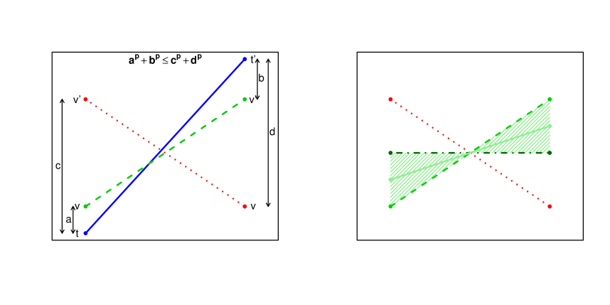
Figure 1. Geometric illustration for the proof of Proposition 1 (left panel) and comparison to isotonic regression (right panel). The solid dark line is the target function $f_{0}$, the dotted line is the original estimate $\hat{f}$, the dashed line is the rearranged estimate $\hat{f}^{\ast}$, the dotted-dashed line is the isotonized estimate $\hat{f}^{I}$, and the solid light line is the average of the rearranged and isotonized estimates $\hat{f}^{1/2}$. In the left panel $L(v,t)=a^{p}$, $L(v^{\prime},t)=c^{p}$, $L(v^{\prime},t^{\prime})=b^{p}$, and $L(v,t^{\prime})=d^{p}$.

Here we informally explain why rearrangement provides the improvement property and compare rearrangement to isotonization.

We begin by noting that the proof of the improvement property can be first reduced to the case of step functions or, equivalently, functions with a finite domain, and then to the case of functions with a two-point domain. The improvement property for such functions then follows from the submodularity property (2.3). In the left panel of Figure 1 we illustrate this geometrically by plotting the original estimate $\hat{f}$, the rearranged estimate $\hat{f}^{*}$, and the true function $f_{0}$. In this example, the original estimate is decreasing and hence violates the monotonicity requirement. We see that the two-point rearrangement co-monotonizes $\hat{f}^{*}$ with $f_{0}$ and thus brings $\hat{f}^{*}$ closer to $f_{0}$. Also, we can view the rearrangement as a projection on the set of weakly increasing functions that have the same distribution as the original estimate $\hat{f}$.

In the right panel of Fig. 1 we plot both the rearranged and isotonized estimates. The isotonized estimate $\hat{f}^{I}$ is a projection of the original estimate $\hat{f}$ on the set of weakly increasing functions, that only preserves the mean of the original estimate. We can compute the two values of the isotonized estimate $\hat{f}^{I}$ by assigning to both the average of the two values of the original estimate $\hat{f}$, whenever the latter violate the monotonicity requirement, and leaving the original values unchanged otherwise. In our example in Fig. 1 this produces a flat function $\hat{f}^{I}$. This pool adjacent violators procedure extends to domains with more than two points by applying the procedure iteratively to any pair of points at which monotonicity is violated [PAVA1955].

Using the computational definition of isotonization, one can show that, like rearrangement, isotonization also improves upon the original estimate, for any $p\in[1,\infty]$:

$$\left\{\int_{\mathcal{X}}|\hat{f}^{I}(x)-f_{0}(x)|^{p}dx\right\}^{1/p}\leq\left\{\int_{\mathcal{X}}|\hat{f}(x)-f_{0}(x)|^{p}dx\right\}^{1/p},$$

see, e.g., barlow:book. Therefore, it follows that any function $\hat{f}^{\lambda}$ in the convex hull of the rearranged and isotonized estimate both (1) monotonizes and (2) improves upon the original estimate $\hat{f}$, that is, for any $p\in[1,\infty]$ and $\lambda\in[0,1]$,

$$\left\{\int_{\mathcal{X}}|\hat{f}^{\lambda}(x)-f_{0}(x)|^{p}dx\right\}^{1/p}\leq\ \ \left\{\int_{\mathcal{X}}|\hat{f}(x)-f_{0}(x)|^{p}dx\right\}^{1/p},$$

where $\hat{f}^{\lambda}=\lambda\hat{f}^{*}+(1-\lambda)\hat{f}^{I}$. The first property is obvious and the second follows from homogeneity and subadditivity of norms. By induction on the dimension, the improvement property extends to the sequential multivariate isotonization and to its convex hull with the sequential multivariate rearrangement.

Thus, we see that a rather rich class of procedures both monotonizes the original estimate and reduces the distance to the true target function. However, there is no single best distance-reducing monotonizing procedure. Indeed, whether the rearranged estimate $\hat{f}^{*}$ approximates the target function better than the isotonized estimate $\hat{f}^{I}$ depends on how steep or flat the target function is. We illustrate this point using the example plotted in the right panel of Fig. 1: consider any increasing target function taking values in the shaded area between $\hat{f}^{*}$ and $\hat{f}^{I}$, and also the function $\hat{f}^{1/2}$, the average of the isotonized and the rearranged estimate, that passes through the middle of the shaded area. Suppose first that the target function is steeper than $\hat{f}^{1/2}$, then $\hat{f}^{*}$ has a smaller estimation error than $\hat{f}^{I}$. Now suppose instead that the target function is flatter than $\hat{f}^{1/2}$, then $\hat{f}^{I}$ has a smaller estimation error than $\hat{f}^{*}$. It is also clear that, if the target function is neither very steep nor very flat, $\hat{f}^{1/2}$ can outperform either $\hat{f}^{*}$ or $\hat{f}^{I}$. Thus, in practice we can choose rearrangement, isotonization, or, some combination of the two, depending on our beliefs about how steep or flat the target function is in a particular application.

3. Improving Interval Estimates of Monotone Functions by Rearrangement

In this section we propose to directly apply the rearrangement, univariate and multivariate, to simultaneous confidence intervals for monotone functions. We show that our proposal will necessarily improve the original intervals by decreasing their length while retaining the same or greater coverage level.

Suppose that we are given an initial simultaneous confidence interval

$$[\ell,u]=\{[\ell(x),u(x)],x\in\mathcal{X}^{d}\},$$ (3.1)

where $\ell$ and $u$ are the lower and upper end-point functions such that $\ell\leq u$ on $\mathcal{X}^{d}$, that is, $\ell(x)\leq u(x)$ for all $x\in\mathcal{X}^{d}$. We further suppose that the confidence interval $[\ell,u]$ has either the exact or the asymptotic confidence property for the estimand function $f$, namely, for a given $\alpha\in(0,1)$,

$$\text{pr}_{P}\{f\in[\ell,u]\}\geq 1-\alpha,$$ (3.2)

for all probability measures $P$ in some set $\mathcal{P}_{n}$ containing the true probability measure $P_{0}$. The statement $f\in[\ell,u]$ means that $\ell(x)\leq f(x)\leq u(x)$ for all $x\in\mathcal{X}^{d}$. We assume that property (3.2) holds either in the finite sample sense, that is, for the given sample size $n$, or in the asymptotic sense, that is, for all but finitely many sample sizes $n$ [LR2005].

A common confidence interval for functions specifies

$$\ell(x)=\hat{f}(x)-\hat{c}s(x),\ \ \ \ \ u(x)=\hat{f}(x)+\hat{c}s(x),$$ (3.3)

where $\hat{f}(x)$ is a point estimate, $s(x)$ is the standard error of the point estimate, and $\hat{c}$ is a critical value chosen to attain the confidence property (3.2). Wasserman06 provides an excellent overview of methods for constructing the critical value. The problem with such confidence intervals, as with the point estimates themselves, is that they need not be monotonic. Indeed, the end-point functions (3.3) need not be monotonic, so the confidence interval may contain non-monotone functions excludable from it. Accordingly we can intersect the interval with the set of monotone functions to reduce its length without affecting its coverage level. In some cases, however, the initial interval may not contain any monotone function and the resulting intersected interval is empty, due, for example, to misspecification.

We say that confidence intervals are misspecified or incorrectly centered if the estimand $f$, being covered by $[\ell,u]$ in (3.2), is not equal to the weakly increasing target function $f_{0}$, so that $f$ may not be monotone. Incorrect centering is rather common both in parametric and non-parametric estimation. In parametric estimation correct centering of confidence intervals requires perfect specification of functional forms, whereas in nonparametric estimation correct centering requires the so-called undersmoothing; both are difficult. In real applications with many regressors, researchers tend to use oversmoothing rather than undersmoothing. In a recent development, GW08 provide some formal justification for oversmoothing: targeting inference on functions $f$, that represent various smoothed versions of $f_{0}$ and thus summarize features of $f_{0}$, may be desirable to make inference more robust, or, equivalently, to enlarge the class of data-generating processes $\mathcal{P}_{n}$ for which (3.2) holds. Regardless of the reasons for why the confidence intervals may target $f$ instead of $f_{0}$, our procedures will work for inference on the monotonized, hence improved, version $f^{*}$ of $f$.

Our proposal for improved interval estimates is to rearrange the entire simultaneous confidence interval into a monotonic interval

$$[\ell^{*},u^{*}]=\{[\ell^{*}(x),u^{*}(x)],x\in\mathcal{X}^{d}\},$$ (3.4)

where the lower and upper end-point functions $\ell^{*}$ and $u^{*}$ are the increasing rearrangements of the original end-point functions $\ell$ and $u$. In the multivariate case, we use the symbols $\ell^{*}$ and $u^{*}$ to denote either multivariate $\pi$-rearrangements $\ell_{\pi}^{*}$ and $u_{\pi}^{*}$ or average multivariate rearrangements $\ell^{*}$ and $u^{*}$, whenever we do not need to emphasize specifically the dependence on $\pi$.

The following proposition describes the properties of the rearranged confidence intervals.

Proposition 3.

Let $[\ell,u]$ in (3.1) be the original confidence interval satisfying the property (3.2) for the estimand function $f:\mathcal{X}^{d}\mapsto K$ and let the rearranged confidence interval $[\ell^{*},u^{*}]$ be defined as in (3.4).

1. The interval $[\ell^{*},u^{*}]$ is weakly increasing and non-empty, in the sense that the end-point functions $\ell^{*}$ and $u^{*}$ are weakly increasing on $\mathcal{X}^{d}$ and satisfy $\ell^{*}\leq u^{*}$ on $\mathcal{X}^{d}$. Moreover, the event that $f\in[\ell,u]$ implies the event that $f^{*}\in[\ell^{*},u^{*}].$ In particular, under the correct specification, when $f$ equals a weakly increasing target function $f_{0}$, we have that $f=f^{*}=f_{0}$, so that $f_{0}\in[\ell,u]$ implies $f_{0}\in[\ell^{*},u^{*}].$ Therefore, $[\ell^{*},u^{*}]$ covers $f^{*}$, which is equal to $f_{0}$ under the correct specification, with a probability that is greater or equal to the probability that $[\ell,u]$ covers $f$.

2. The interval $[\ell^{*},u^{*}]$ is weakly shorter than $[\ell,u]$ in the $L^{p}$ length: for each $p\in[1,\infty]$,

$$\left\{\int_{\mathcal{X}^{d}}\Big{|}\ell^{*}(x)-u^{*}(x)\Big{|}^{p}dx\right\}^{1/p}\leq\left\{\int_{\mathcal{X}^{d}}\Big{|}\ell(x)-u(x)\Big{|}^{p}dx\right\}^{1/p}.$$ (3.5)

3. In the univariate case, suppose that there exist subsets $\mathcal{X}_{0}\subset\mathcal{X}$ and $\mathcal{X}^{\prime}_{0}\subset\mathcal{X}$, each of measure greater than $\delta>0$ such that for all $x^{\prime}\in\mathcal{X}^{\prime}_{0}$ and $x\in\mathcal{X}_{0}$, we have that $x^{\prime}>x$, and either (i) $\ell(x)>\ell(x^{\prime})+\epsilon$, and $u(x^{\prime})>u(x)+\epsilon$, for some $\epsilon>0$ or (ii) $\ell(x^{\prime})>\ell(x)+\epsilon$ and $u(x)>u(x^{\prime})+\epsilon$, for some $\epsilon>0$. Then, for any $p\in(1,\infty)$,

$$\left\{\int_{\mathcal{X}}\Big{|}\ell^{*}(x)-u^{*}(x)\Big{|}^{p}dx\right\}^{1/p}\leq\left\{\int_{\mathcal{X}}\Big{|}\ell(x)-u(x)\Big{|}^{p}-\eta_{p}\delta\right\}^{1/p},$$

where $\eta_{p}=\inf\{|v-t^{\prime}|^{p}+|v^{\prime}-t|^{p}-|v-t|^{p}-|v^{\prime}-t^{\prime}|^{p}\}>0$, where the infimum is taken over all $v,v^{\prime},t,t^{\prime}$ in $K$ such that $v^{\prime}\geq v+\epsilon$ and $t^{\prime}\geq t+\epsilon$.

In the multivariate case with $d\geq 2$, for an ordering $\pi=(\pi_{1},\ldots,\pi_{k},\ldots,\pi_{d})$ of integers $\{1,\ldots,d\}$ with $\pi_{k}=j$, let $\bar{g}$ denote the partially rearranged function, $\bar{g}=R_{\pi_{k+1}}\ldots R_{\pi_{d}}\hat{g}$, where for $k=d$ we set $\bar{g}=\hat{g}$. Suppose there exist subsets $\mathcal{X}_{j}\subset\mathcal{X}$ and $\mathcal{X}_{j}^{\prime}\subset\mathcal{X}$, each of measure greater than $\delta>0$, and a subset $\mathcal{X}_{-j}\subseteq\mathcal{X}^{d-1}$, of measure $\nu>0$, such that for all $x=(x_{j},x_{-j})$ and $x^{\prime}=(x^{\prime}_{j},x_{-j})$, with $x_{j}^{\prime}\in\mathcal{X}_{j}^{\prime}$, $x_{j}\in\mathcal{X}_{j}$, $x_{-j}\in\mathcal{X}_{-j}$, we have that (i) $x_{j}^{\prime}>x_{j}$, and either (ii) $\bar{\ell}(x)>\bar{\ell}(x^{\prime})+\epsilon$, and $\bar{u}(x^{\prime})>\bar{u}(x)+\epsilon$, for some $\epsilon>0$ or (iii) $\bar{\ell}(x^{\prime})>\bar{\ell}(x)+\epsilon$ and $\bar{u}(x)>\bar{u}(x^{\prime})+\epsilon$, for some $\epsilon>0$. Then, for any $p\in(1,\infty)$ and $\eta_{p}>0$ defined as above

$$\left\{\int_{\mathcal{X}^{d}}\Big{|}\ell^{*}_{\pi}(x)-u^{*}_{\pi}(x)\Big{|}^{p}dx\right\}^{1/p}\leq\left\{\int_{\mathcal{X}^{d}}\Big{|}\ell(x)-u(x)\Big{|}^{p}-\eta_{p}\delta\nu\right\}^{1/p}.$$

Proposition 3 shows that the rearranged confidence intervals are weakly shorter than the original confidence intervals, and also qualifies when the rearranged confidence intervals are strictly shorter. In particular, in the univariate case the inequality (3.5) is necessarily strict for $p\in(1,\infty)$ if there is a region of positive measure in $\mathcal{X}$ over which the end-point functions $\ell$ and $u$ are not comonotonic. This weak shortening result follows for univariate cases directly from the Lorentz (1953) inequality, and the strong shortening by its strengthening. The shortening results for the multivariate case follow by induction on the dimension. Moreover, the order-preservation property of the univariate and multivariate rearrangements, demonstrated in the proof, implies that the rearranged confidence interval $[\ell^{*},u^{*}]$ has a weakly higher coverage than the original confidence interval $[\ell,u]$. We do not quantify strict improvements in coverage, but demonstrate them through the examples in the next section.

Our idea of directly monotonizing the interval estimates also applies to other monotonization procedures. Indeed, the proof of Proposition 3 reveals that part 1 applies to any order-preserving monotonization operator $T$, such that

$$g\leq m\text{ implies }Tg\leq Tm.$$ (3.6)

Furthermore, part 2 of Proposition 3 on the weak shortening of the confidence intervals applies to any distance-reducing operator $T$ such that

$$\left\{\int_{\mathcal{X}^{d}}|T\ell(x)-Tu(x)|^{p}dx\right\}^{1/p}\leq\left\{\int_{\mathcal{X}^{d}}|\ell(x)-u(x)|^{p}dx\right\}^{1/p}.$$ (3.7)

Rearrangements are instances of operators that have properties (3.6) and (3.7). Isotonization is another important instance [RWD88]. Moreover, convex combinations of order-preserving and distance-reducing operators, such as the average of rearrangement and isotonization, also have properties (3.6) and (3.7).

4. Illustrations

4.1. An empirical illustration with age-height reference charts

In this section we provide an empirical application to biometric age-height charts. We show how the rearrangement monotonizes and improves various nonparametric point and interval estimates for functions.

Since their introduction by Quetelet in the 19th century, reference growth charts have become common tools to assess an individual’s health status. These charts describe the evolution of individual anthropometric measures, such as height, weight, and body mass index, across different ages. See cole for a classical work on the subject, and koenker:charts for a recent analysis from a quantile regression perspective and additional references. Here we consider an application of the rearrangement and other related methods to the estimation of growth charts for height. This makes sense since an individual’s height should follow an increasing relationship with age up to adulthood. Our data consist of repeated cross sectional measurements of height in centimeters and age in months from the 2003-2004 US National Health and Nutrition Survey, and is further restricted to the subsample of US-born white males aged 2-20 to avoid other confounding factors, giving us a sample of 533 observations.

Let $Y$ and $X$ denote height and age, respectively. Let $E[Y\mid X=x]$ denote the conditional expectation of $Y$ given $X=x$, and $Q_{Y}[u\mid X=x]$ denote the conditional $u$-th quantile of $Y$ given $X=x$, where $u$ is the quantile index. The target functions of interests are the conditional expectation function, $x\mapsto E[Y\mid X=x]$, the conditional quantile functions for several quantile indices, $x\mapsto Q_{Y}[u\mid X=x]$, for $u=5\%$, $50\%$, and $95\%$, and the entire conditional quantile process for height given age, $(u,x)\mapsto Q_{Y}[u\mid X=x]$. The monotonicity requirements for these target functions are the following: the first two should be increasing in age $x$, and the third should be increasing in both age $x$ and the quantile index $u$.

We estimate the target functions using non-parametric ordinary least squares or quantile regression and then rearrange the estimates to satisfy the monotonicity requirements. We consider kernel, local linear, regression splines, and Fourier series methods. For the kernel and local linear methods, we choose a bandwidth of one year and a box kernel. For the regression splines method, we use cubic B-splines with a knot sequence $\{3,5,8,10,11.5,13,14.5,16,18\}$ [koenker:charts]. For the Fourier method, we employ four sines and four cosines. For the estimation of the conditional quantile process, we use $\{0.005,0.010,\ldots,0.995\}$ as a net of quantile indices.

Figure 2 shows the original and rearranged estimates of the conditional quantile functions for the different methods. All the estimated curves have trouble capturing the slowdown in the growth of height after age fifteen and yield non-monotonic curves for the highest values of age. The Fourier series performs particularly poorly in approximating the aperiodic age-height relationship and has many non-monotonicities. The rearrangement delivers curves that improve upon the original estimates and that satisfy the natural monotonicity requirement. We quantify this improvement in the next subsection.

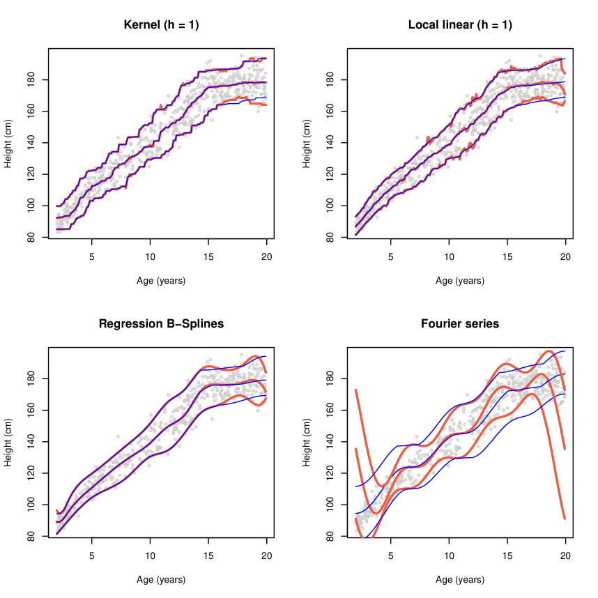
Figure 2. Estimates of the 5%, 50%, and 95% conditional quantile functions of height given age and their increasing rearrangements, obtained by kernel, local linear, cubic B-splines series, and Fourier series regression. Light thick lines are the original estimates and dark thin lines are the rearranged estimates.

Figure 4 (a,b) illustrates the multivariate rearrangement of the conditional quantile process along both the age and the quantile index arguments. We plot, in three dimensions, the original estimate and its average multivariate rearrangement (the average of the age-quantile and quantile-age rearrangements). We focus on the Fourier series estimates, which have the most severe non-monotonicity problems. Analogous figures for the other estimation methods are given in an MIT working paper containing an extended version of this article. We see that the estimated quantile process is non-monotone in age and in the quantile index at extremal values of this index. The average multivariate rearrangement fixes the non-monotonicity problem delivering an estimate of the quantile process that is monotone in both the age and the quantile index. Furthermore, by the theoretical results of the paper, the multivariate rearranged estimates necessarily improve upon the original estimates.

In Figures 3 and 4 (c,d), we plot original and rearranged 90% simultaneous confidence intervals. Fig. 3 shows the intervals for the conditional expectation function and for the conditional 5%, 50%, and 95% quantile functions, based on Fourier series estimates. We obtain the original intervals of the form (3.3) using the bootstrap with 200 repetitions to estimate the standard errors and critical values [Hall1993]. We then obtain the rearranged confidence intervals by rearranging the lower and upper end-point functions of the initial confidence intervals, following Section 3. In Fig. 4 (c,d), we plot the original and the rearranged 90% simultaneous confidence intervals for the entire conditional quantile process, based on the Fourier series estimates. The rearranged confidence intervals correct the non-monotonicity of the original confidence intervals and reduce their integrated $L^{p}$ length.

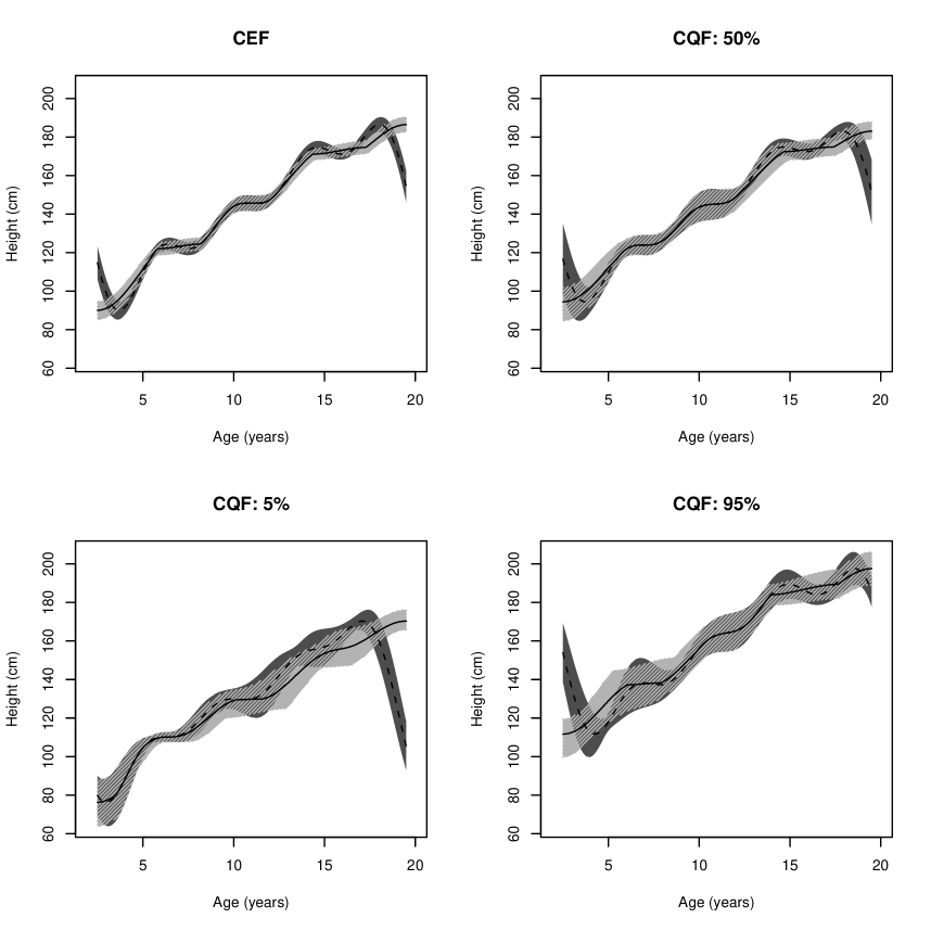
Figure 3. 90% confidence intervals for conditional expectation function (CEF), and 5%, 50% and 95% conditional quantile functions (CQF) of height given age and their increasing rearrangements. Estimates are based on Fourier series and confidence bands are obtained by bootstrap with 200 repetitions. Dark bands are the original confidence intervals and light bands are the rearranged confidence intervals.

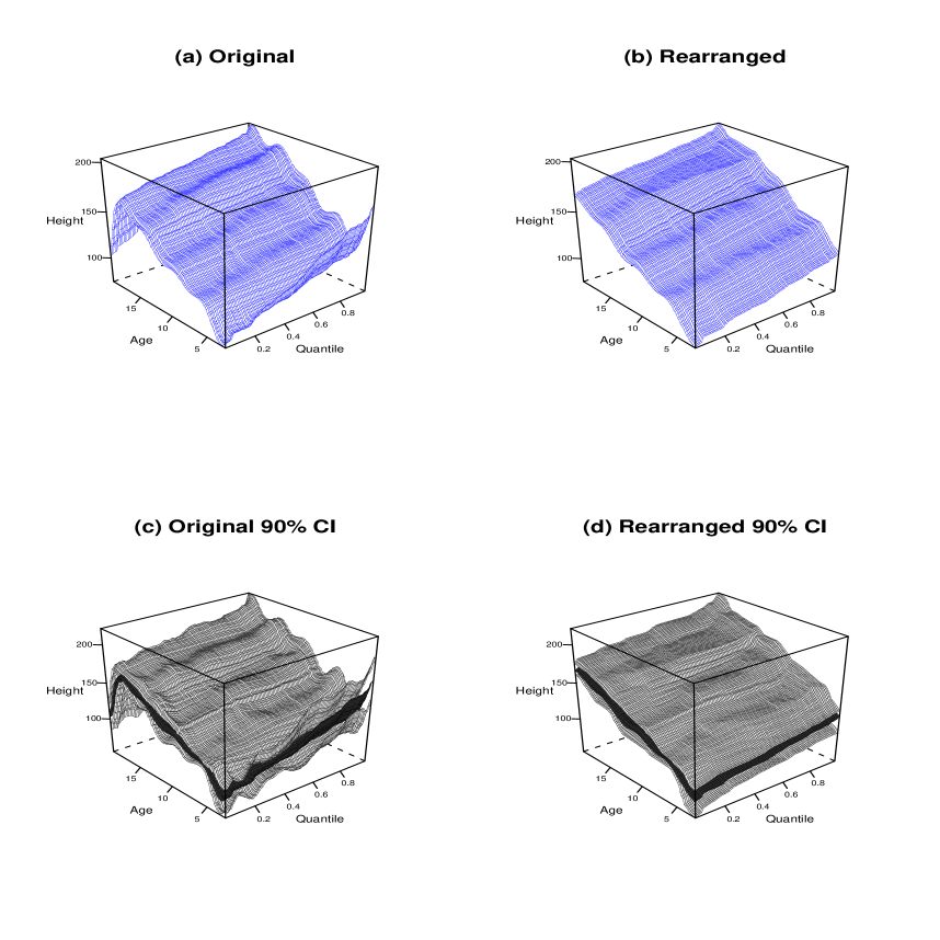
Figure 4. Fourier series point and interval estimates of the conditional quantile process of height given age and their increasing rearrangements. Panels (a) and (b) plot original estimate and its average multivariate rearrangement. Panels (c) and (d) plot original and rearranged 90% confidence intervals. Original confidence interval obtained by bootstrap with 200 repetitions.

4.2. Monte-Carlo illustration

In the following Monte Carlo experiment we quantify the improvement in the point and interval estimation that rearrangement can provide relative to the original estimates. We also compare it to isotonization and to its convex combinations with isotonization. Our experiment uses a model, described in detail in the Appendix, that mimics the empirical application very closely. This model implies a true conditional expectation function and quantile process that are monotone in age and in the quantile index.

In Table 1 we report the average $L^{p}$ errors, for $p=1,2,$ and $\infty$, for the original estimates of the conditional expectation function. We also report the relative efficiency of the rearranged estimates, measured as the ratio of the average error of the rearranged estimate to the average error of the original estimate; together with relative efficiencies for alternative approaches based on isotonization of the original estimates [Mammen1991] and on averaging the rearranged and isotonized estimates. For regression splines, we also consider the one-step monotone regression splines [Ramsay1998].

For all of the methods and norms considered, the rearranged curves estimate the target function more accurately than the original curves. There is no uniform winner between rearrangement, isotonization, and the average of the two, which is consistent with the analysis of Section 2.4. For example, the rearrangement outperforms the other methods for kernel, local linear and splines, but performs worse than the average for Fourier in some norms. In numerical results not reported, we find that rearrangement performs worse than isotonization for global polynomials. This and other methods are available in the MIT working paper. For regression splines, the performance of the rearrangement is comparable to the computationally more intensive one-step monotone splines procedure.

Table 1. $L^{p}$ Estimation Errors of Original, Rearranged, Isotonized, Average Rearranged-Isotonized, and Monotone Estimates of the Conditional Expectation Function, for $p=1,2$, $\infty$.

$p$	$\ \ L^{p}_{O}\ \$	$L^{p}_{R}/L^{p}_{O}$	$L^{p}_{I}/L^{p}_{O}$	$L^{p}_{(R+I)/2}/L^{p}_{O}$	$L^{p}_{M}/L^{p}_{O}$		$\ \ L^{p}_{O}\ \$	$L^{p}_{R}/L^{p}_{O}$	$L^{p}_{I}/L^{p}_{O}$	$L^{p}_{(R+I)/2}/L^{p}_{O}$
	Kernel						Local linear
$1$	1$\cdot$00	0$\cdot$97	0$\cdot$98	0$\cdot$98	–		0$\cdot$79	0$\cdot$96	0$\cdot$97	0$\cdot$96
$2$	1$\cdot$30	0$\cdot$98	0$\cdot$99	0$\cdot$98	–		0$\cdot$99	0$\cdot$96	0$\cdot$97	0$\cdot$97
$\infty$	4$\cdot$54	0$\cdot$99	1$\cdot$00	1$\cdot$00	–		2$\cdot$93	0$\cdot$95	0$\cdot$95	0$\cdot$95
	Regression splines						Fourier
$1$	0$\cdot$87	0$\cdot$93	0$\cdot$95	0$\cdot$94	0$\cdot$99		6$\cdot$57	0$\cdot$49	0$\cdot$59	0$\cdot$40
$2$	1$\cdot$09	0$\cdot$93	0$\cdot$95	0$\cdot$94	0$\cdot$99		10$\cdot$8	0$\cdot$35	0$\cdot$45	0$\cdot$30
$\infty$	3$\cdot$68	0$\cdot$85	0$\cdot$88	0$\cdot$86	0$\cdot$84		48$\cdot$9	0$\cdot$16	0$\cdot$34	0$\cdot$20

$L^{p}_{O}$, $L^{p}_{R}$,$L^{p}_{I}$, $L^{p}_{(R+I)/2}$, and $L^{p}_{M}$ are average $L^{p}$ errors of the original, rearranged, isotonized, the average rearranged-isotonized, and monotone regression splines estimates; they are computed as the Monte Carlo average of $\{\int_{\mathcal{X}}|\bar{f}(x)-f_{0}(x)|^{p}dx\}^{1/p},$ where $f_{0}$ is the target and $\bar{f}$ an estimate.

In Table 2 we report the average $L^{p}$ errors for the original estimates of the conditional quantile process. We also report the ratio of the average error of the multivariate rearranged estimate, with respect to the age and quantile index arguments, to the average error of the original estimate; together with the same ratios for isotonized and average rearranged-isotonized estimates. We obtain the multivariate isotonized estimates by sequentially applying the univariate isotonization to each argument, and then averaging for the two possible orderings age-quantile and quantile-age. For all the methods and norms considered, the multivariate rearranged curves estimate the target function more accurately than the original curves. There is again no uniform winner between rearrangement, isotonization, and their average.

Table 2. $L^{p}$ Estimation Errors of Original, Rearranged, Isotonized, and Average Rearranged-Isotonized Estimates of the Conditional Quantile Process, for $p=1,2,$ and $\infty$.

$p$		$\ \ L^{p}_{O}\ \$	$L^{p}_{R}/L^{p}_{O}$	$L^{p}_{I}/L^{p}_{O}$	$L^{p}_{(R+I)/2}/L^{p}_{O}$		$\ \ L^{p}_{O}\ \$	$L^{p}_{R}/L^{p}_{O}$	$L^{p}_{I}/L^{p}_{O}$	$L^{p}_{(R+I)/2}/L^{p}_{O}$
		Kernel					Local linear
$1$		1$\cdot$49	0$\cdot$95	0$\cdot$97	0$\cdot$96		1$\cdot$21	0$\cdot$91	0$\cdot$93	0$\cdot$92
$2$		1$\cdot$99	0$\cdot$96	0$\cdot$98	0$\cdot$97		1$\cdot$61	0$\cdot$91	0$\cdot$93	0$\cdot$92
$\infty$		13$\cdot$7	0$\cdot$92	0$\cdot$97	0$\cdot$94		12$\cdot$3	0$\cdot$84	0$\cdot$87	0$\cdot$85
		Regression splines					Fourier
$1$		1$\cdot$33	0$\cdot$90	0$\cdot$93	0$\cdot$91		6$\cdot$72	0$\cdot$62	0$\cdot$77	0$\cdot$64
$2$		1$\cdot$78	0$\cdot$90	0$\cdot$92	0$\cdot$90		13$\cdot$7	0$\cdot$39	0$\cdot$58	0$\cdot$44
$\infty$		16$\cdot$9	0$\cdot$72	0$\cdot$76	0$\cdot$73		84$\cdot$9	0$\cdot$26	0$\cdot$47	0$\cdot$36

$L^{p}_{O}$, $L^{p}_{R}$,$L^{p}_{I}$, and $L^{p}_{(R+I)/2}$ are the average $L^{p}$ errors of the original, multivariate rearranged, multivariate isotonized, the multivariate average rearranged-isotonized estimates; they are computed as the Monte Carlo averages of $\{\int_{\mathcal{U}}\int_{\mathcal{X}}|\bar{f}(u,x)-f_{0}(u,x)|^{p}dxdu\}^{1/p},$ where $f_{0}$ is the target and $\bar{f}$ an estimate.

Table 3 reports Monte Carlo coverage frequencies and integrated lengths for the original and monotonized 90% confidence bands for the conditional expectation function. For a measure of length, we used the integrated $L^{p}$ length, as defined in Proposition 3, with $p=1,2,$ and $\infty$. We construct the original confidence intervals of the form specified in equations (3.3) by obtaining the pointwise standard errors of the original estimates using the bootstrap with 200 repetitions, and calibrate the critical value so that the original confidence bands cover the entire true function with the exact frequency of 90%. We construct monotonized confidence intervals by applying rearrangement, isotonization, and a rearrangement-isotonization average to the end-point functions of the original confidence intervals, as proposed in Section 3. In all cases the rearrangement and other monotonization methods increase the coverage of the confidence intervals while reducing their length. In particular, we see that monotonization increases coverage especially for the local estimation methods, whereas it reduces length most noticeably for the global estimation methods. For the most problematic Fourier estimates, there are large increases in coverage and reductions in length.

Table 3. Coverage (%) and Integrated Lengths of Original, Rearranged, Isotonized, and Average Rearranged-Isotonized 90% Confidence Intervals for the Conditional Expectation Function.

Interval	Cover	Length				Cover	Length
		$\ \ L^{1}\ \$	$L^{1}/L^{1}_{O}$	$L^{2}/L^{2}_{O}$	$L^{\infty}/L^{\infty}_{O}$		$\ \ L^{1}\ \$	$L^{1}/L^{1}_{O}$	$L^{2}/L^{2}_{O}$	$L^{\infty}/L^{\infty}_{O}$
	Kernel					Local linear
$O$	90	8$\cdot$80				90	8$\cdot$63
$R$	96	8$\cdot$79	1	1	0$\cdot$99	96	8$\cdot$63	1	1	0$\cdot$97
$I$	94	8$\cdot$80	1	1	0$\cdot$99	94	8$\cdot$63	1	1	0$\cdot$98
$(R+I)/2$	95	8$\cdot$80	1	1	0$\cdot$99	95	8$\cdot$63	1	1	0$\cdot$97
	Regression splines					Fourier
$O$	90	6$\cdot$32				90	24$\cdot$91
$R$	91	6$\cdot$32	1	1	1	100	24$\cdot$52	0$\cdot$98	0$\cdot$94	0$\cdot$63
$I$	91	6$\cdot$32	1	1	1	100	24$\cdot$91	1	0$\cdot$97	0$\cdot$69
$(R+I)/2$	91	6$\cdot$32	1	1	1	100	24$\cdot$71	0$\cdot$99	0$\cdot$95	0$\cdot$65

$O$, $R$, $I$, and $(R+I)/2$ refer to original, rearranged, isotonized, and average rearranged-isotonized confidence intervals. Coverage probabilities (Cover) are for the entire function.

Appendix A Proofs of Propositions

Proof of Proposition 1

Proof of Part 1. This follows in part the strategy in Lorentz’s (1953) proof. We assume first that the functions $\hat{f}$ and $f_{0}$ are step functions, constant on intervals $((s-1)/r,s/r]$, $s=1,\ldots,r$. For each step function $f$ with $r$ steps we associate an $r$-vector $f$ whose $s$-th element, denoted $f_{s}$, equals to the value of function $f$ on the $s$-th interval, and vice versa. Let us define the sorting operator $S$ acting on vectors (and functions) $f$ as follows. Let $k$ be an integer in $1,\ldots,r$ such that $f_{k}>f_{m}$ for some $m>k$. If $k$ does not exist, set $Sf=f$. If $k$ exists, set $Sf$ to be a $r$-vector with the $k$-th element equal to $f_{m}$, the $m$-th element equal to $f_{k}$, and all other elements equal to the corresponding elements of $f$. Finally, given a vector $Sf$ there is a step function $Sf$ associated to it, as stated above.

For any submodular function $L:\mathbb{R}^{2}\to\mathbb{R}_{+}$, by $f_{k}\geq f_{m}$, $f_{0m}\geq f_{0k}$ and the definition of the submodularity, $L(f_{m},f_{0k})+L(f_{k},f_{0m})\leq L(f_{k},f_{0k})+L(f_{m},f_{0m}).$ A simple geometric illustration for this property is given in Figure 1. Therefore, conclude that $\int_{\mathcal{X}}L\{S\hat{f}(x),f_{0}(x)\}dx\leq\int_{\mathcal{X}}L\{\hat{f}(x),f_{0}(x)\}dx,$ using that we integrate step functions. Applying the sorting operator a sufficient finite number of times to $\hat{f}$, we obtain a completely sorted, that is, rearranged, vector $\hat{f}^{*}$. Thus, we can express $\hat{f}^{*}$ as $\hat{f}^{*}=S\ldots S\hat{f}$, where the operator $S$ is applied finitely many times. By repeating the argument above, each application weakly reduces the estimation error. Therefore,

$$\int_{\mathcal{X}}L\{\hat{f}^{*}(x),f_{0}(x)\}dx\leq\int_{\mathcal{X}}L\{S\ldots S\hat{f}(x),f_{0}(x)\}dx\leq\int_{\mathcal{X}}L\{\hat{f}(x),f_{0}(x)\}dx.$$ (A.1)

Next we extend this result to general measurable functions $\hat{f}$ and $f_{0}$ mapping $[0,1]$ to $K$, where $f_{0}$ is a quantile function. Take a subsequence of bounded step functions $\hat{f}^{(q)}$ and $f_{0}^{(q)}$, with $f_{0}^{(q)}$ being quantile functions, converging to $\hat{f}$ and $f_{0}$ almost everywhere as index $q\to\infty$ along an increasing sequence of integers. The almost everywhere convergence of $\hat{f}^{(q)}$ to $\hat{f}$ implies the almost everywhere convergence of its quantile function $\hat{f}^{*(q)}$ to the quantile function of the limit, $\hat{f}^{*}$ (vaart:text, p. 305). Since (A.1) holds for each $q$ along the subsequence, the dominated convergence theorem implies that (A.1) also holds for the general case.

It remains to show the existence of the subsequence in the preceding paragraph. Using series expansion in the Haar basis, any function in $L^{2}[0,1]$ can be approximated in $L^{2}$ norm by a sequence of $r$-step functions, where $r=2^{j}$ and $j=1,\ldots,\infty$ (pollard:measure, p. 305) . Hence there is a subsequence of step functions $\hat{f}^{(r)}$ and $f^{(r)}_{0}$ converging to $\hat{f}$ and $f_{0}$ in $L^{2}$ norm; the functions in the subsequence necessarily take values in $K$; by pollard:measure, p. 38, we can extract a further subsequence $\hat{f}^{(q)}$ and $f^{(q)}_{0}$, with $q$ running over an increasing sequence of integers, converging to $\hat{f}$ and $f_{0}$ almost everywhere. Finally, replace $f^{(q)}_{0}$ by their quantile functions, i.e., rearrangements, which retain the almost everywhere convergence property to $f_{0}$ by vaart:text, p. 305. ∎

Proof of Part 2. Consider the step functions, as defined in the proof of Part 1. By setting $r$ sufficiently large, we can take them to satisfy the following hypotheses: there exist regions $\mathcal{X}_{0}$ and $\mathcal{X}^{\prime}_{0}$, each of measure greater than $\delta>0$, such that for all $x\in\mathcal{X}_{0}$ and $x^{\prime}\in\mathcal{X}_{0}^{\prime}$, we have that (i) $x^{\prime}>x$, (ii) $\hat{f}(x)>\hat{f}(x^{\prime})+\epsilon$, and (iii) $f_{0}(x^{\prime})>f_{0}(x)+\epsilon$, for $\epsilon>0$ specified in the proposition. For any strictly submodular function $L:\mathbb{R}^{2}\to\mathbb{R}_{+}$ we have that $\eta=\inf\{L(v^{\prime},t)+L(v,t^{\prime})-L(v,t)-L(v^{\prime},t^{\prime})\}>0,$ where the infimum is taken over all $v,v^{\prime},t,t^{\prime}$ in the set $K$ such that $v^{\prime}\geq v+\epsilon$ and $t^{\prime}\geq t+\epsilon$. We can begin sorting by exchanging an element $\hat{f}(x)$, $x\in\mathcal{X}_{0}$, of $r$-vector $\hat{f}$ with an element $\hat{f}(x^{\prime})$, $x^{\prime}\in\mathcal{X}_{0}^{\prime}$, of $r$-vector $\hat{f}$. This induces a sorting gain of at least $\eta$ times $1/r$. The total mass of points that can be sorted in this way is at least $\delta$. We then proceed to sort all of these points in this way, and then continue with the sorting of other points. After the sorting is completed, the total gain from sorting is at least $\delta\eta$. That is, $\int_{\mathcal{X}}L\{\hat{f}^{*}(x),f_{0}(x)\}dx\leq\int_{\mathcal{X}}L\{\hat{f}(x),f_{0}(x)\}dx-\delta\eta.$

We then extend this inequality to the general measurable functions exactly as in the proof of Part 1. ∎

Proof of Proposition 2

Proof of Part 1. We prove the claim by induction. It is true for $d=1$ by $\hat{f}^{*}$ being a quantile function. Suppose the claim is true in $d-1\geq 1$ dimensions. If so, then $x_{-j}\mapsto\bar{f}(x_{j},x_{-j})$, obtained from the original estimate $\hat{f}$ after applying the rearrangement to all arguments $x_{-j}$ of $x$, except for the argument $x_{j}$, must be weakly increasing in $x_{-j}$ for each $x_{j}$. Thus, for any $x_{-j}^{\prime}\geq x_{-j}$ and $X_{j}\sim U[0,1]$, we have

$$\bar{f}(X_{j},x_{-j}^{\prime})\geq\bar{f}(X_{j},x_{-j}).$$ (A.2)

Therefore, the random variable on the left of (A.2) dominates the random variable on the right of (A.2) in the stochastic sense. Therefore, the quantile function of the random variable on the left dominates the quantile function of the random variable on the right, namely $\bar{f}^{*}_{j}(x_{j},x_{-j}^{\prime})\geq\bar{f}^{*}_{j}(x_{j},x_{-j})\text{ for each }x_{j}\in\mathcal{X}=[0,1].$ Moreover, for each $x_{-j}$, the function $x_{j}\mapsto\bar{f}^{*}_{j}(x_{j},x_{-j})$ is weakly increasing by virtue of being a quantile function. We conclude therefore that $x\mapsto\bar{f}_{j}^{*}(x)$ is weakly increasing in all of its arguments at all points $x\in\mathcal{X}^{d}$. The claim of Part 1 of the Proposition now follows by induction. ∎

Proof of Part 2 (a). By Proposition 1, we have that for each $x_{-j}$,

$$\begin{split}\int_{\mathcal{X}}\left|\bar{f}_{j}^{*}(x_{j},x_{-j})-f_{0}(x_{j},x_{-j})\right|^{p}dx_{j}\leq\int_{\mathcal{X}}\left|\bar{f}(x_{j},x_{-j})-f_{0}(x_{j},x_{-j})\right|^{p}dx_{j}.\end{split}$$ (A.3)

Now, the claim follows by integrating with respect to $x_{-j}$ and taking the $p$-th root of both sides. For $p=\infty$, the claim follows by taking the limit as $p\to\infty$. ∎

Proof of Part 2 (b). We first apply the inequality of Part 2(a) to $\bar{f}(x)=\hat{f}(x)$, then to $\bar{f}(x)=R_{\pi_{d}}\hat{f}(x),$ then to $\bar{f}(x)=R_{\pi_{d-1}}R_{\pi_{d}}\hat{f}(x)$, and so on. In doing so, we recursively generate a sequence of weak inequalities that imply the inequality (2.4) stated in the Proposition. ∎

Proof of Part 3 (a). For each $x_{-j}\in\mathcal{X}^{d-1}\setminus\mathcal{X}_{-j}$, by Part 2(a), we have the weak inequality (A.3), and for each $x_{-j}\in\mathcal{X}_{-j}$, by the inequality for the univariate case stated in Proposition 1 Part 2, we have the strong inequality

$$\begin{split}\int_{\mathcal{X}}\left|\bar{f}_{j}^{*}(x_{j},x_{-j})-f_{0}(x_{j},x_{-j})\right|^{p}dx_{j}\leq\int_{\mathcal{X}}\left|\bar{f}(x_{j},x_{-j})-f_{0}(x_{j},x_{-j})\right|^{p}dx_{j}-\eta_{p}\delta,\end{split}$$ (A.4)

where $\eta_{p}$ is defined in the same way as in Proposition 1. Integrating the weak inequality (A.3) over $x_{-j}\in\mathcal{X}^{d-1}\setminus\mathcal{X}_{-j}$, of measure $1-\nu$, and the strong inequality (A.4) over $\mathcal{X}_{-j}$, of measure $\nu$, we obtain

$$\begin{split}\int_{\mathcal{X}^{d}}\left|\bar{f}_{j}^{*}(x)-f_{0}(x)\right|^{p}dx\leq\int_{\mathcal{X}^{d}}\left|\bar{f}(x)-f_{0}(x)\right|^{p}dx-\eta_{p}\delta\nu.\end{split}$$ (A.5)

The claim now follows. ∎

Proof of Part 3 (b). As in Part 2(a), we can recursively obtain a sequence of weak inequalities describing the improvements in estimation error from rearranging sequentially with respect to the individual arguments. Moreover, at least one of the inequalities can be strengthened to be of the form stated in (A.5), from the assumption of the claim. The resulting system of inequalities yields the inequality (2.5), stated in the proposition. ∎

Proof of Part 4. This part follows from homogeneity and subadditivity of the $L_{p}$ norm. ∎

Proof of Proposition 3

Proof of Part 1. The monotonicity follows from Proposition 2. The rest of the proof relies on establishing the order-preserving property of the $\pi$-rearrangement operator: for any measurable functions $g,m:\mathcal{X}^{d}\to\mathbb{R}$, we have that $g(x)\leq m(x)$ for all $x\in\mathcal{X}^{d}$ implies $g^{*}(x)\leq m^{*}(x)$ for all $x\in\mathcal{X}^{d}.$ Given the property we have that $\ell(x)\leq f(x)\leq u(x)\text{ for all }x\in\mathcal{X}^{d}\text{ implies }\ell^{*}(x)\leq f^{*}(x)\leq u^{*}(x)\text{ for all }x\in\mathcal{X}^{d},$ which verifies the claim of the first part. The claim also extends to the average multivariate rearrangement, since averaging preserves the order-preserving property.

It remains to establish the order-preserving property for $\pi-$rearrangement, which we do by induction. We first note that in the univariate case, when $d=1$, order preservation is obvious from the rearrangement being a quantile function: the random variable $m(X)$, where $X\sim U[0,1]$, dominates the random variable $g(X)$ in the stochastic sense, hence the quantile function $m^{*}(x)$ of $m(X)$ must be weakly greater than the quantile function $g^{*}(x)$ of $g(X)$ for each $x\in\mathcal{X}$. We then extend this to the multivariate case by induction: Suppose the order-preserving property is true for any $d-1\geq 1$. If so, then, for each $x_{j}\in\mathcal{X}$ and $x_{-j}\in\mathcal{X}^{d-1}$, $g(x_{j},x_{-j})\leq m(x_{j},x_{-j})\text{ implies }\bar{g}(x_{j},x_{-j})\leq\bar{m}(x_{j},x_{-j}),$ where $\bar{g}$ and $\bar{m}$ are multivariate rearrangements of $x_{-j}\mapsto g(x_{j},x_{-j})$ and $x_{-j}\mapsto m(x_{j},x_{-j})$ with respect to $x_{-j}$, holding $x_{j}$ fixed. Now apply the order-preserving property of the univariate rearrangement to the univariate functions $x_{j}\mapsto\bar{g}(x_{j},x_{-j})$ and $x_{j}\mapsto\bar{m}(x_{j},x_{-j})$, holding $x_{-j}$ fixed, for each $x_{-j}$, to conclude that the order-preserving property holds for dimension $d$.∎

Proof of Part 2. As stated in the text, the weak inequality follows from Lorentz (1953). For completeness we only briefly note that the proof follows similarly to the proof of Proposition 1. Indeed, we can start with step functions $\ell$ and $u$ and work with their equivalent vector representations $\ell$ and $u$. Then we apply the sorting operator $S_{2}$ to the pair of $r$-vectors $(\ell,u)$ defined as $S_{2}(\ell,u)=(S\ell,S^{\prime}u)$, where $S$ is the sorting operator on the vector $\ell$ defined in the proof of Proposition 1, and $S^{\prime}$ is a subordinated sorting operator on the vector $u$ defined by two conditions: (1) if $S$ exchanges the $k$-th and $m$-th elements of $\ell$, where $m>k$, then, if $u_{k}>u_{m}$, $S^{\prime}$ also exchanges the $k$-th and $m$-th elements of $u$ , and if $u_{k}\leq u_{m}$, $S^{\prime}$ leaves all elements of $u$ unchanged; and (2) if $S$ exchanges no elements of $\ell$, i.e., $S\ell=\ell$, then $S^{\prime}$ is simply the unrestricted $S$ operator as defined in the proof of Proposition 1, i.e., $S^{\prime}=S$. By the definition of submodularity (2.3), each application of $S_{2}$ weakly reduces submodular discrepancies between vectors, so that the pairs of vectors in the sequence $\{(\ell,u),S_{2}(\ell,u),\ldots,S_{2}\ldots S_{2}(\ell,u),(\ell^{*},u^{*})\}$ become progressively weakly closer to each other, and the sequence can be taken to be finite, where the last pair is the rearrangement $(\ell^{*},u^{*})$ of vectors $(\ell,u)$. The inequality extends to general bounded measurable functions by passing to the limit using a similar argument to the proof of Proposition 1. The extension of the proof to the multivariate case follows by induction on the dimension, as in the proof of Proposition 2. ∎

Proof of Part 3. Finally, the proof of strict inequality in the univariate case is similar to the proof of Proposition 2, using the fact that for strictly submodular functions $L:\mathbb{R}^{2}\mapsto\mathbb{R}_{+}$ we have that $\eta=\inf\{L(v^{\prime},t)+L(v,t^{\prime})-L(v,t)-L(v^{\prime},t^{\prime})\}>0,$ where the infimum is taken over all $v,v^{\prime},t,t^{\prime}$ in the set $K$ such that $v^{\prime}\geq v+\epsilon$ and $t^{\prime}\geq t+\epsilon$ or such that $v\geq v^{\prime}+\epsilon$ and $t\geq t^{\prime}+\epsilon$. The extension of the strict inequality to the multivariate case follows exactly as in the proof of Proposition 2. ∎

Appendix B Design of the Monte-Carlo experiment

The outcome variable $Y$ equals a location function plus a disturbance $\epsilon$, $Y=Z(X)^{\prime}\beta+\epsilon,$ and the disturbance is independent of the regressor $X$. The vector $Z(X)$ includes a constant and a piecewise linear transformation of the regressor $X$ with three changes of slope, namely $Z(X)=(1,X,1\{X>5\}(X-5),1\{X>10\}(X-10),1\{X>15\}(X-15))$. This design implies the conditional expectation function $E[Y\mid X]=Z(X)^{\prime}\beta$, and the conditional quantile function $Q_{Y}[u\mid X]=Z(X)^{\prime}\beta+Q_{\epsilon}(u).$ We select the parameters of the design to match the growth charts example. Thus, we set the parameter $\beta$ equal to the ordinary least squares estimate obtained in the growth chart data, namely ($71.25$, $8.13$, $-2.72$, $1.78$, $-6.43$). This parameter value and the location specification imply a model for the conditional expectation function and quantile process that is monotone for ages 2-20. To generate the values of the dependent variable, we draw disturbances from a normal distribution whose mean and variance match those of the estimated residuals, $\epsilon=Y-Z(X)^{\prime}\beta$. We fix the values of the regressor $X$ to be the observed values of age in the data. In each replication, we estimate the target functions using the nonparametric methods described in Section 4.1. The total number of replications is 1000. All computations were carried out using the software R [R2007], the quantile regression package quantreg, and the functional data analysis package fda. The rearrangement method developed in this paper is available in the package rearrangement for R.

References

- [1] \harvarditem[Andrews]Andrews1991andrews:series Andrews, D. W. K. (1991): “Asymptotic normality of series estimators for nonparametric and semiparametric regression models,” Econometrica, 59(2), 307–345.
- [2] \harvarditem[Ayer, Brunk, Ewing, Reid, and Silverman]Ayer, Brunk, Ewing, Reid, and Silverman1955PAVA1955 Ayer, M., H. D. Brunk, G. M. Ewing, W. T. Reid, and E. Silverman (1955): “An empirical distribution function for sampling with incomplete information,” Ann. Math. Statist., 26, 641–647.
- [3] \harvarditem[Barlow, Bartholomew, Bremner, and Brunk]Barlow, Bartholomew, Bremner, and Brunk1972barlow:book Barlow, R. E., D. J. Bartholomew, J. M. Bremner, and H. D. Brunk (1972): Statistical inference under order restrictions. The theory and application of isotonic regression. John Wiley & Sons, New York.
- [4] \harvarditem[Chaudhuri]Chaudhuri1991chaudhuri:1991 Chaudhuri, P. (1991): “Nonparametric estimates of regression quantiles and their local Bahadur representation,” Ann. Statist., 19, 760–777.
- [5] \harvarditem[Chernozhukov, Fernandez-Val, and Galichon]Chernozhukov, Fernandez-Val, and Galichon2006CFG-RE-ET Chernozhukov, V., I. Fernandez-Val, and A. Galichon (2006): “Rearranging Edgeworth-Cornish-Fisher Expansions,” Forthcoming in Economic Theory.
- [6] \harvarditem[Cole]Cole1988cole Cole, T. J. (1988): “Fitting smoothed centile curves to reference data,” J Royal Stat Soc, 151, 385–418.
- [7] \harvarditem[Davydov and Zitikis]Davydov and Zitikis2005DZ2005 Davydov, Y., and R. Zitikis (2005): “An index of monotonicity and its estimation: a step beyond econometric applications of the Gini index,” Metron, 63(3), 351–372.
- [8] \harvarditem[Dette, Neumeyer, and Pilz]Dette, Neumeyer, and Pilz2006dette1 Dette, H., N. Neumeyer, and K. F. Pilz (2006): “A simple nonparametric estimator of a strictly monotone regression function,” Bernoulli, 12(3), 469–490.
- [9] \harvarditem[Dette and Scheder]Dette and Scheder2006dette3 Dette, H., and R. Scheder (2006): “Strictly monotone and smooth nonparametric regression for two or more variables,” The Canadian Journal of Statistics, 34(4), 535–561.
- [10] \harvarditem[Fan and Gijbels]Fan and Gijbels1996fan:book Fan, J., and I. Gijbels (1996): Local polynomial modelling and its applications, vol. 66 of Monographs on Statistics and Applied Probability. Chapman & Hall, London.
- [11] \harvarditem[Fougeres]Fougeres1997fougeres1997 Fougeres, A.-L. (1997): “Estimation de densites unimodales,” The Canadian Journal of Statistics / La Revue Canadienne de Statistique, 25(3), 375–387.
- [12] \harvarditem[Gallant]Gallant1981gallant:fourier Gallant, A. R. (1981): “On the bias in flexible functional forms and an essentially unbiased form: the Fourier flexible form,” J. Econometrics, 15(2), 211–245.
- [13] \harvarditem[Genovese and Wasserman]Genovese and Wasserman2008GW08 Genovese, C., and L. Wasserman (2008): “Adaptive confidence bands,” Ann. Statist., 36(2), 875–905.
- [14] \harvarditem[Hall]Hall1993Hall1993 Hall, P. (1993): “On Edgeworth Expansion and Bootstrap Confidence Bands in Nonparametric Curve Estimation,” Journal of the Royal Statistical Society. Series B (Methodological), 55(1), 291–304.
- [15] \harvarditem[Hardy, Littlewood, and Pólya]Hardy, Littlewood, and Pólya1952HLP52 Hardy, G. H., J. E. Littlewood, and G. Pólya (1952): Inequalities. Cambridge University Press, 2d ed.
- [16] \harvarditem[He and Shao]He and Shao2000he:series He, X., and Q.-M. Shao (2000): “On parameters of increasing dimensions,” J. Multivariate Anal., 73(1), 120–135.
- [17] \harvarditem[Koenker and Bassett]Koenker and Bassett1978koenker:1978 Koenker, R., and G. S. Bassett (1978): “Regression quantiles,” Econometrica, 46, 33–50.
- [18] \harvarditem[Koenker and Ng]Koenker and Ng2005koenker:inequality Koenker, R., and P. Ng (2005): “Inequality constrained quantile regression,” Sankhyā, 67(2), 418–440.
- [19] \harvarditem[Lehmann and Romano]Lehmann and Romano2005LR2005 Lehmann, E. L., and J. P. Romano (2005): Testing statistical hypotheses. Springer, New York, third edn.
- [20] \harvarditem[Lorentz]Lorentz1953lorentz:1953 Lorentz, G. G. (1953): “An inequality for rearrangements,” Amer. Math. Monthly, 60, 176–179.
- [21] \harvarditem[Mammen]Mammen1991Mammen1991 Mammen, E. (1991): “Nonparametric Regression Under Qualitative Smoothness Assumptions,” Ann. Stat., 19(2), 741–759.
- [22] \harvarditem[Mammen, Marron, Turlach, and Wand]Mammen, Marron, Turlach, and Wand2001MMTW2001 Mammen, E., J. S. Marron, B. A. Turlach, and M. P. Wand (2001): “A general projection framework for constrained smoothing,” Statist. Sci., 16(3), 232–248.
- [23] \harvarditem[Matzkin]Matzkin1994matzkin:handbook Matzkin, R. L. (1994): “Restrictions of economic theory in nonparametric methods,” in Handbook of econometrics, Vol. IV, vol. 2 of Handbooks in Econom., pp. 2523–2558. North-Holland, Amsterdam.
- [24] \harvarditem[Newey]Newey1997newey:series Newey, W. K. (1997): “Convergence rates and asymptotic normality for series estimators,” J. Econometrics, 79(1), 147–168.
- [25] \harvarditem[Pollard]Pollard2002pollard:measure Pollard, D. (2002): A user’s guide to measure theoretic probability, vol. 8 of Cambridge Series in Statistical and Probabilistic Mathematics. Cambridge University Press, Cambridge.
- [26] \harvarditem[Portnoy]Portnoy1997portnoy:splines Portnoy, S. (1997): “Local asymptotics for quantile smoothing splines,” Ann. Statist., 25(1), 414–434.
- [27] \harvarditem[R Development Core Team]R Development Core Team2008R2007 R Development Core Team (2008): R: A Language and Environment for Statistical ComputingR Foundation for Statistical Computing, Vienna, Austria, ISBN 3-900051-07-0.
- [28] \harvarditem[Ramsay]Ramsay1988Ramsay1988 Ramsay, J. O. (1988): “Monotone Regression Splines in Action,” Stat. Science, 3(4), 425–441.
- [29] \harvarditem[Ramsay]Ramsay1998Ramsay1998 (1998): “Estimating smooth monotone functions,” J. Royal Stat. Soc: B, 60(2), 365–375.
- [30] \harvarditem[Ramsay and Silverman]Ramsay and Silverman2005silverman:book Ramsay, J. O., and B. W. Silverman (2005): Functional data analysis. Springer, New York, second edn.
- [31] \harvarditem[Robertson, Wright, and Dykstra]Robertson, Wright, and Dykstra1988RWD88 Robertson, T., F. T. Wright, and R. L. Dykstra (1988): Order restricted statistical inference. John Wiley & Sons Ltd., Chichester.
- [32] \harvarditem[Silvapulle and Sen]Silvapulle and Sen2005silvapulle:book Silvapulle, M. J., and P. K. Sen (2005): Constrained statistical inference. John Wiley & Sons, Hoboken, NJ.
- [33] \harvarditem[Stone]Stone1994Stone:series Stone, C. J. (1994): “The use of polynomial splines and their tensor products in multivariate function estimation,” Ann. Statist., 22(1), 118–184, With discussion by Andreas Buja and Trevor Hastie and a rejoinder by the author.
- [34] \harvarditem[van der Vaart]van der Vaart1998vaart:text van der Vaart, A. W. (1998): Asymptotic statistics. Cambridge University Press, Cambridge.
- [35] \harvarditem[Villani]Villani2003villani Villani, C. (2003): Topics in optimal transportation, vol. 58 of Graduate Studies in Mathematics. American Mathematical Society, Providence, RI.
- [36] \harvarditem[Wand and Jones]Wand and Jones1995wand:jones Wand, M. P., and M. C. Jones (1995): Kernel smoothing, vol. 60 of Monographs on Statistics and Applied Probability. Chapman and Hall Ltd., London.
- [37] \harvarditem[Wasserman]Wasserman2006Wasserman06 Wasserman, L. (2006): All of nonparametric statistics, Springer Texts in Statistics. Springer, New York.
- [38] \harvarditem[Wei, Pere, Koenker, and He]Wei, Pere, Koenker, and He2006koenker:charts Wei, Y., A. Pere, R. Koenker, and X. He (2006): “Quantile regression methods for reference growth charts,” Stat. Med., 25(8), 1369–1382.
- [39]