Malleable Coding: Compressed Palimpsests

Abstract

A malleable coding scheme considers not only compression efficiency but also the ease of alteration, thus encouraging some form of recycling of an old compressed version in the formation of a new one. Malleability cost is the difficulty of synchronizing compressed versions, and malleable codes are of particular interest when representing information and modifying the representation are both expensive. We examine the trade-off between compression efficiency and malleability cost under a malleability metric defined with respect to a string edit distance. This problem introduces a metric topology to the compressed domain. We characterize the achievable rates and malleability as the solution of a subgraph isomorphism problem. This can be used to argue that allowing conditional entropy of the edited message given the original message to grow linearly with block length creates an exponential increase in code length.

I Introduction

The source coding theorem for block codes is obtained by calculating the number of typical source sequences and generating a set of labels to enumerate them. Asymptotically almost surely (a.a.s), only typical sequences will occur so it is sufficient that the set of labels be as large as the set of typical sequences; this yields the achievable entropy bound. As Shannon comments, “The high probability group is coded in an arbitrary one-to-one way into this set,” and so in this sense there is no notion of topology of typical sequences.

If one is concerned with zero error rather than a.a.s. negligible error, the source coding theorem for variable-length codes also yields the entropy as an achievable lower bound. In this setting, the mapping from source sequences to labels is not allowed to be quite as arbitrary; however, as long as an optimizing set of code lengths is correctly matched to source letters, there are still some arbitrary choices in an optimal construction [2].

In contrast to these well-known settings, we investigate the mapping from the source to its compressed representation motivated by the following problem. Suppose that after compressing a source $X_{1}^{n}$, it is modified to become $Y_{1}^{n}$ according to a memoryless editing process $p_{Y|X}$. A malleable coding scheme preserves some portion of the codeword of $X_{1}^{n}$ and modifies the remainder into a new codeword from which $Y_{1}^{n}$ may be decoded reliably.

There are several ways to define how one preserves some portion of the codeword of $X_{1}^{n}$. Here we concentrate on a malleability cost defined by a normalized edit distance in the compressed domain. This is motivated by systems where the old codeword is stored in a rewritable medium; cost is incurred when a symbol has to be changed in value, regardless of the location. Recalling the ancient practice of scraping and overwriting parchment [3], we call the storage medium a compressed palimpsest and the characterization of the trade-offs the palimpsest problem.

A companion paper [4] focuses on a distinct problem with a similar motivation. There, we fix a part of the old codeword to be recycled in creating a codeword for $Y_{1}^{n}$. Without loss of generality, the fixed portion can be taken to be the beginning of the codeword, so the new codeword is a fixed prefix followed by a new suffix. This formulation is suitable for applications in which the update information (new suffix) must be transmitted through a communication channel. If the locations of the changed symbols were to be arbitrary, one would need to assign a cost to the indexing of the locations.

The main result for the palimpsest problem is a graphical characterization of achievable rates and number of editing operations. The result involves the solution to the error-tolerant attributed subgraph isomorphism problem [5], which is essentially a graph embedding problem. Although graph functionals such as independence number [6] and chromatic number [7] often arise in the solution of information theory problems, this seems to be the first time that the subgraph isomorphism problem has arisen. Moreover, this seems to be the first treatment of the source code as a mapping between metric spaces.

Several of the results we obtain are pessimistic. Unless the old source and the new source are very strongly correlated, a large rate penalty must be paid in order to have minimal malleability cost. Similarly, a large malleability cost must be incurred if the rates are required to be close to entropy.

Outline and Preview

The remainder of the paper is organized as follows. In Section II, we present a few toy examples of coding methods that exhibit a large range of possible trade-offs. Section III provides additional motivation and context for our work. Section IV then provides a formal problem statement, and constructive coding techniques paralleling those previewed in Section II are developed precisely in Section V.

In Section VI, graph embedding techniques are used to specify achievable rate–malleability points. In particular, Section VI-A deals with Hamming distance as the editing cost and proposes a construction using Gray codes. Lower bounds and constructive examples using letter-by-letter encoding and decoding are given. This graph embedding approach is generalized in Section VI-C to include other edit distances via generalized minimal change codes.

While the above delay-free encoding and decoding gives optimal results for a few special cases, we consider a more general coding approach in Section VII, considering both variable-length and block codes. In the latter case, we show that the topology of typical sequences plays an important role in our problem. Using graph-theoretic ideas, we give an achievability result in Theorem 2. Further, in Theorem 3 we argue that a linear reduction in malleability is at exponential cost in compression efficiency, consistent with the examples given in Section II. This theorem is proved for “stationary editing distributions,” though we believe it to be true for general distributions. In Theorem 4, we give an upper bound on malleability cost using the Lipschitz constant of the source code mapping for general distributions.

Section VIII provides some final observations on the trade-off between malleability cost and compression efficiency, gives some conclusions, and discusses future work.

II Simple Examples

To motivate this exposition prior to defining all quantities precisely, we begin by giving four examples of how one can trade off between compression efficiency and malleability. Let $X$, $Y$, and $Z$ be binary variables with entropies $H(X)$, $H(Y)$, and $H(Z)$, respectively. Suppose that the original observation is a word $X_{1}^{n}$. After compressing $X_{1}^{n}$, the original source is modified by adding a binary sequence $Z_{1}^{n}$ with Hamming weight $np$ to obtain a new word $Y_{1}^{n}=X_{1}^{n}\oplus Z_{1}^{n}$. Suppose the storage alphabet is also binary and that the cost of synchronization is measured with the extended Hamming distance. Unlike many source coding problems where only the cardinality of the set of codewords is used, here the alphabet itself is used to measure malleability cost; an abstract set of indices is not appropriate.

How might the code for $X_{1}^{n}$ and the update mechanism to allow representation of $Y_{1}^{n}$ be designed? The four possibilities below are summarized in Fig. 1.

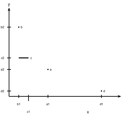
Figure 1: Qualitative representation of the four simple techniques of Section II. For ease of representation, it is assumed that $H(X)=H(Y)$. The relative orderings of points are based on $H(Z)\ll H(X)$; this reflects the natural case where the editing operation is of low complexity relative to the original string.

No compression

We store $n$ bits for $X_{1}^{n}$. Hence synchronizing to the new version only requires changing the same number of bits in the code as were changed from $X_{1}^{n}$ to $Y_{1}^{n}$; the cost is the Hamming weight of $Z_{1}^{n}$, $np$.

Fully compress $X_{1}^{n}$ and $Y_{1}^{n}$

We apply Shannon-type compression, storing only $nH(X)$ bits for $X_{1}^{n}$. It seems, however, that a large portion of this old codeword will have to be changed—perhaps about half the bits—to become a representation for $Y_{1}^{n}$. Compression efficiency is obtained at the cost of malleability.

Fully compress $X_{1}^{n}$ and an increment

Another coding strategy is to compress the change $Z_{1}^{n}$ separately and append it to the original compression of $X_{1}^{n}$. The new compression then has length $n(H(X)+H(Z))\geq nH(Y)$ bits. The extended Hamming malleability cost is $nH(Z)$ bits.

Completely favor malleability over compression

Interestingly, there is a method that dramatically trades compression efficiency for malleability. The source $X_{1}^{n}$ is encoded with $2^{nH(X)}$ bits, using an indicator function to denote which of its typical sequences was observed. The same strategy is used to encode $Y_{1}^{n}$, using $2^{nH(Y)}$ bits. Then synchronization requires changing only two bits when $X_{1}^{n}$ and $Y_{1}^{n}$ are different.

Our purpose is to study the limits of this interesting trade-off between compression efficiency and malleability. We will do so using formalized performance metrics after a bit more background.

III Background

Our study of malleable compression is motivated by information storage systems that store documents which are updated often. In such systems, the storage costs include not only the average length of the coded signal, but also the costs in updating. We describe these systems and also discuss an information storage system in synthetic biology, where the editing costs are much more significant and restrictive than in optical or magnetic systems.

III-A Version Management

Consider the installation of a security patch to an operating system, the update of a text document after proofreading, the storage of a computer file backup system after a day’s work, or a second email that corrects the location of a seminar yet also reproduces the entire seminar abstract. In all of these settings and numerous others, separate data streams may be generated, but the contents differ only slightly [10, 11, 12, 13]. Moreover, in these applications, old versions of the stream need not be preserved. Particularly for devices such as mobile telephones, where memory size and energy are severely constrained, but for any storage system, it is advisable to reduce the space taken by data and also to reduce the energy required to insert, delete, and modify stored data. In certain applications, in-place reconstruction is desired [12], necessitating the use of instantaneous source codes.

Recursive estimation and control also require temporarily storing state estimates and updating them at each time step. Thus such problems also suggest themselves as application areas for malleable coding. Note that the application of malleable codes would determine how information storage is carried out, not what information is stored and what information is dissipated [14].

In the scenarios discussed, new versions will be correlated with old versions, not independent as assumed in previous studies of write-efficient memories [15, 16]. That is, we envision scenarios which involve updating Archimedes of Siracusa with Archimedes of Syracuse (Levenshtein distance $2$) rather than updating with Jesus of Nazareth (Levenshtein distance $15$), though the results will apply to the entire gamut of scenarios.

There is also another difference between the problems we formulate and prior work on write-efficient memories. In write-efficient memories, the encoder can look to see what is already stored in the memory before deciding the codeword for the update. An information pattern even more extensive than for write-efficient memories was discussed in [17]. We require the code to be determined before the encoding process is carried out. Such an information pattern would arise naturally in remote file synchronization [13].

Once the codeword of the new version is determined (without access to the realized compressed old version), there may be settings where the differences between the two must be determined in a distributed fashion. For a good malleable code, the old and new codewords will be strongly correlated. Thus, protocols for distributed reconciliation of correlated strings may be used [18, 19, 13].

III-B Genetic Coding

With recent advances in biotechnology [20], the storage of artificial messages in DNA strings seems like a real possibility, rather than just a laboratory pipe dream [21]. Thus the storage of messages in the DNA of living organisms as a long-lasting, high-density data storage medium provides another motivating application for malleable coding. Note that although minimum change codes, as we will develop for the palimpsest problem, have been suggested as an explanation for the genetic code through the optimization approach to biology [22], here we are concerned with synthetic biology.

As in magnetic or optical storage and perhaps more so, it is desirable to compress information for storage. For a palimpsest system, one would use site-directed mutagenesis [23, Ch. 7] to perform editing of stored codewords whereas for the formulation of malleable coding in [4], molecular biology cloning techniques using restriction enzymes, oligonucleotide synthesis or polymerase chain reaction (PCR), and ligation [23, Ch. 3] would be used. In site-directed mutagenesis when multiple changes cannot be made using a single primer, the cost of a single insertion, deletion, or substitution is approximately the same and is additive with respect to the number of edits. Using restriction enzyme methods with oligonucleotide synthesis, however, the cost is related to the length of the new segment that must be synthesized to replace the old segment. Thus the biotechnical editing costs correspond exactly to the costs defined in the present paper and in [4]. Unlike magnetic or optical storage, insertion and deletion are natural operations in DNA information storage, thereby allowing variable-length codes to be easily edited. Incidentally, insertion and deletion is also possible in neural information storage through modification of neuronal arbors [24].

IV Problem Statement

After a few requisite definitions, we will provide a formal statement of the palimpsest problem, which takes editing costs as well as rate costs into account.

The symbols of the storage medium are drawn from the finite alphabet $\mathcal{V}$. Note that unlike most source coding problems, the alphabet itself will be used, not just the cardinality of sequences drawn from this alphabet. Also, it is natural to measure all rates in numbers of symbols from $\mathcal{V}$. This is analogous to using base-$|\mathcal{V}|$ logarithms in place of base-2 logarithms, and all logarithms should be interpreted as such.

We require the notion of an edit distance [25] on $\mathcal{V}^{*}$, the set of all finite sequences of elements of $\mathcal{V}$.

Definition 1

An edit distance, $d(\cdot,\cdot)$, is a function from $\mathcal{V}^{*}\times\mathcal{V}^{*}$ to $[0,\infty)$, defined by a set of edit operations. The edit operations are a symmetric relation on $\mathcal{V}^{*}\times\mathcal{V}^{*}$. The edit distance between $a\in\mathcal{V}^{*}$ and $b\in\mathcal{V}^{*}$ is $0$ if $a=b$ and is the minimum number of edit operations needed to transform $a$ into $b$ otherwise.

An example of an edit distance is the Levenshtein distance, which is constructed from insertion, deletion, and substitution operations. It can be noted that $(\mathcal{V}^{*},d)$ is a finite metric space (see Appendix A).

Now we can formally define our coding problem. We define the variable-length and block coding versions together, drawing distinctions only where necessary. Symbols are reused so as to conserve notation. It should be clear from context whether we are discussing variable-length or block coding.

Let $\{(X_{i},Y_{i})\}_{i=1}^{\infty}$ be a sequence of independent drawings of a pair of random variables $(X,Y)$, $X\in\mathcal{W}$, $Y\in\mathcal{W}$, where $\mathcal{W}$ is a finite set and $p_{X,Y}(x,y)=\Pr[X=x,Y=y]$. The marginal distributions are

$$p_{X}(x)=\sum_{y\in\mathcal{W}}p_{X,Y}(x,y)$$

and

$$p_{Y}(y)=\sum_{x\in\mathcal{W}}p_{X,Y}(x,y)\mbox{.}$$

When the random variable is clear from context, we write $p_{X}(x)$ as $p(x)$ and so on.

A modification channel

$$p_{Y|X}(y|x)=\frac{p(x,y)}{p(x)}$$

relates the two marginal distributions. If the joint distribution is such that the marginals are equal, the modification channel is said to perform stationary editing.

Variable-length Codes

A variable-length encoder with block length $n$ is a mapping

$$f_{E}:\mathcal{W}^{n}\to\mathcal{V}^{*}\mbox{,}$$

and the corresponding decoder with block length $n$ is

$$f_{D}:\mathcal{V}^{*}\to\mathcal{W}^{n}\mbox{.}$$

The encoder and decoder define a variable-length palimpsest code. The encoder and decoder pair is required to be instantaneous, in the sense that the encoding may be parsed as a succession of codewords.

A (variable-length) encoder-decoder with block length $n$ is applied as follows. Let

$$(A,B)=(f_{E}(X_{1}^{n}),f_{E}(Y_{1}^{n}))\mbox{,}$$

inducing random variables $A$ and $B$ that are drawn from the alphabet $\mathcal{V}^{*}$. Also let

$$(\hat{X}_{1}^{n},\hat{Y}_{1}^{n})=(f_{D}(A),f_{D}(B))\mbox{.}$$

Block Codes

A block encoder for $X$ with parameters $(n,K)$ is a mapping

$$f_{E}^{(X)}:\mathcal{W}^{n}\to\mathcal{V}^{nK}\mbox{,}$$

and a block encoder for $Y$ with parameters $(n,L)$ is a mapping

$$f_{E}^{(Y)}:\mathcal{W}^{n}\to\mathcal{V}^{nL}\mbox{.}$$

Given these encoders, a common decoder with parameter $n$ is

$$f_{D}:\mathcal{V}^{*}\to\mathcal{W}^{n}\mbox{.}$$

The encoders and decoder define a block palimpsest code. Since there is a common decoder, the two codes should be in the same format.

A (block) encoder-decoder with parameters $(n,K,L)$ is applied as follows. Let

$$(A,B)=(f_{E}^{(X)}(X_{1}^{n}),f_{E}^{(Y)}(Y_{1}^{n}))\mbox{,}$$

inducing random variables $A\in\mathcal{V}^{nK}$ and $B\in\mathcal{V}^{nL}$. The mappings are depicted in Fig. 2. Also let

$$(\hat{X}_{1}^{n},\hat{Y}_{1}^{n})=(f_{D}(A),f_{D}(B))\mbox{.}$$

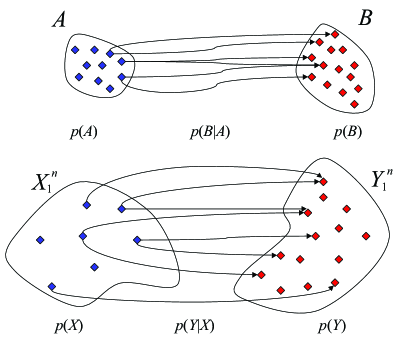
Figure 2: Distributions in representation space induced by distributions in source space.

For both variable-length and block coding, we can define the error rate as

$$\Delta=\max(\Delta_{X},\Delta_{Y})\mbox{,}$$

where

$$\Delta_{X}=\Pr[X_{1}^{n}\neq\hat{X}_{1}^{n}]$$

and

$$\Delta_{Y}=\Pr[Y_{1}^{n}\neq\hat{Y}_{1}^{n}]\mbox{.}$$

Natural (and completely conventional) performance indices for the code are the per-letter average lengths of the codewords

$$K=\frac{1}{n}E\left[\ell(A)\right]\mbox{,}$$

and

$$L=\frac{1}{n}E\left[\ell(B)\right]\mbox{,}$$

where $\ell(\cdot)$ denotes the length of a sequence in $\mathcal{V}^{*}$. (In the block coding case, $A$ has a fixed length of $nK$ letters from the alphabet $\mathcal{V}$, so there is no contradiction in using the previously-defined symbol $K$. Similarly for $L$.)

The final performance measure captures our novel concern with the cost of changing the compressed version. The malleability cost is the expected per-source-letter edit distance between the codes:

$$M=\frac{1}{n}E\left[d(A,B)\right]\mbox{.}$$

Definition 2

Given a source $p(X,Y)$ and an edit distance $d$, a triple $(K_{0},L_{0},M_{0})$ is said to be achievable for the variable-length palimpsest problem if, for arbitrary $\epsilon>0$, there exists (for $n$ sufficiently large) a variable-length palimpsest code with error rate $\Delta=0$, average codeword lengths $K\leq K_{0}+\epsilon$, $L\leq L_{0}+\epsilon$, and malleability $M\leq M_{0}+\epsilon$.

Definition 3

Given a source $p(X,Y)$ and an edit distance $d$, a triple $(K_{0},L_{0},M_{0})$ is said to be achievable for the block palimpsest problem if, for arbitrary $\epsilon>0$, there exists (for $n$ sufficiently large) a block palimpsest code with error rate $\Delta<\epsilon$, average codeword lengths $K\leq K_{0}+\epsilon$, $L\leq L_{0}+\epsilon$, and malleability $M\leq M_{0}+\epsilon$.

For the variable-length palimpsest problem, the set of achievable rate–malleability triples is denoted by $\mathfrak{P}_{V}$; for the block version, the corresponding set is denoted by $\mathfrak{P}_{B}$. It will be our purpose to characterize $\mathfrak{P}_{V}$ and $\mathfrak{P}_{B}$ as much as possible.

It follows from the definition that $\mathfrak{P}_{V}$ and $\mathfrak{P}_{B}$ are closed subsets of $\mathbb{R}^{3}$ and have the property that if $(K_{0},L_{0},M_{0})\in\mathfrak{P}$, then $(K_{0}+\epsilon_{1},L_{0}+\epsilon_{2},M_{0}+\epsilon_{3})\in\mathfrak{P}$ for any $\epsilon_{i}\geq 0$, $i=1,2,3$. Consequently, $\mathfrak{P}_{V}$ and $\mathfrak{P}_{B}$ are completely defined by their lower boundaries, which too are closed.

Both versions of the palimpsest problem can be viewed using the diagram in Fig. 3. Given $p(X,Y)$ and thus $p(X)$, $p(Y)$, and $p(Y|X)$, the malleability constraint defines what is achievable in terms of $p(A,B)$ with the additional constraints that there must be maps between $X_{1}^{n}$ and $A$, and between $Y_{1}^{n}$ and $B$, which allow for lossless or near lossless compression. An alternative formulation as the mapping between two metric spaces $\mathcal{W}^{n}$ and $\mathcal{V}^{*}$ is also possible.

Figure 3: Commutative diagram for the palimpsest problem.

V Constructive Palimpsest Examples

Having formulated the palimpsest problem in Section IV, we present some examples of what can be achieved. These examples revisit Section II. New examples given in Section VI will inspire general statements.

V-A Source Coding with No Compression

The simplest compression scheme is one that simply copies the source sequences to the storage medium. This is only possible when $\mathcal{W}=\mathcal{V}$. When $\mathcal{W}\neq\mathcal{V}$, zero-error coding without compression is possible with block lengths larger than 1, as in converting hexadecimal digits to binary digits or vice versa. The flexibility in such a mapping can be exploited. If the shortest possible blocking is used and $l$ is the least common multiple of $|\mathcal{V}|$ and $|\mathcal{W}|$, then there are $l!$ valid mappings. For the moment, we ignore the gains to be had by exploiting this flexibility and focus on the $\mathcal{W}=\mathcal{V}$ case, with block length $n=1$.

Taking $A=X$ and $B=Y$, it follows immediately that $K=1$ and $L=1$. It also follows that the malleability cost is $M=E[d(X,Y)]$. If we take the edit distance to be the Hamming distance, then $M=\Pr[X\neq Y]$. Thus the triple $(K,L,M)=(1,1,\Pr[X\neq Y])$ is achievable by no compression for any source distribution $p(X,Y)$ under Hamming edit distance.

V-B Ignore Malleability

Consider what happens when the malleability parameter is ignored and the rates for the variable-length encoder are optimized. We will improve rate performance and hopefully not worsen malleability too much.

If the updating process $p_{Y|X}$ is stationary, then a common instantaneous code may be used to asymptotically achieve $K=H(X)$ and $L=H(Y)$. Picking a single code for different sources has been well-studied in the source coding literature, starting with [26]. If a single source code is used for a collection of distributions, the rate loss over the entropy lower bound is termed the redundancy [27]. As shown by Gilbert, if Huffman or Shannon codes are used, this redundancy is the relative entropy between the source and the random variable used to design the code.

Restricting to such instantaneous codes, if the palimpsest code is designed for either $p(x)$ or for $p(y)$, the incurred redundancies are the relative entropies

$$D(p_{X}\|p_{Y})=\sum\limits_{x\in\mathcal{W}}p(x)\log\frac{p(x)}{p(y)}$$

or

$$D(p_{Y}\|p_{X})=\sum\limits_{y\in\mathcal{W}}p(y)\log\frac{p(y)}{p(x)}$$

respectively. These lead to horizontal and vertical portions of a lower bound for $\mathfrak{P}_{V}$ in the $K$–$L$ plane.

An intermediary portion of this lower bound, between the vertical and horizontal portions, is determined by finding a random variable $Z$ that is between $X$ and $Y$ and designing a code for it. We want to choose some “tilted” distribution, $p_{Z}$, on the geodesic between the two distributions $p_{X}$ and $p_{Y}$.

If $p_{Z}=\tfrac{1}{2}p_{X}+\tfrac{1}{2}p_{Y}$, then $D(p_{X}\|p_{Z})+D(p_{Y}\|p_{Z})$ is called the capacitory discrimination [28]. The rate loss in the balanced rate loss case, $D(p_{X}\|p_{Z})$ when $D(p_{X}\|p_{Z})=D(p_{Y}\|p_{Z})$, has a closed form expression [29]. The distribution $p_{Z}$ used to achieve it is halfway (in the asymmetric sense of $Y$ after $X$) along the geodesic that connects the two distributions. The distance along the geodesic may be parameterized by

$$t=\frac{D(p_{Y}\|p_{X})}{D(p_{Y}\|p_{X})+D(p_{X}\|p_{Y})}\mbox{.}$$

The resulting rate loss for $Z_{t}$ is

$$D(p_{X}\|p_{Z_{t}})=R(p_{X},p_{Y})+\log\mu(t)\mbox{,}$$

where $R(p_{X},p_{Y})$ is defined through

$$\frac{1}{R(p_{X},p_{Y})}=\frac{1}{D(p_{X}\|p_{Y})}+\frac{1}{D(p_{Y}\|p_{X})}\mbox{,}$$

and

$$\mu(t)=\sum\limits_{x\in\mathcal{W}}p_{X}^{1-t}(x)p_{Y}^{t}(x)\mbox{.}$$

Notice that due to the asymmetry of the relative entropy, this is different than the Chernoff information. In general, the connecting portion between the horizontal and vertical parts of the lower bound is curved below the time-sharing line, determined by the relative entropies $D(p_{X}\|p_{Z})$ and $D(p_{Y}\|p_{Z})$ for a $Z$ that is along the geodesic connecting the two distributions. Fig. 4 shows an example of this achievable lower bound.

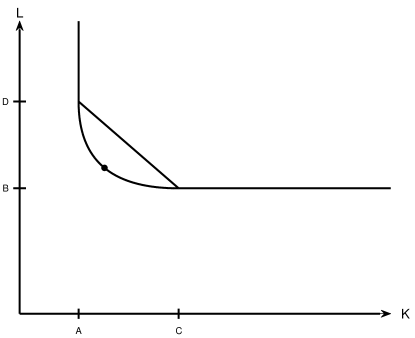
Figure 4: $K$–$L$ region achievable using instantaneous codes for sources related through non-stationary editing. The marked point is when rate loss for both versions is balanced. The diagonal line segment shows the suboptimal strategy of time-sharing.

If the restriction to instantaneous codes is removed, then there are several kinds of universal source codes that achieve the $K\geq H(X)$ and $L\geq H(Y)$ bounds simultaneously [27, 30], however instantaneous codes are required by the palimpsest problem statement. These results say nothing about $M$, they only deal with $K$ and $L$.

To say something about $M$, one can show that the average starting overlap is rather small [31]. Since optimal source codes produce equiprobable outputs [32], one might hope that computing $M$ is a matter of measuring the expected edit distance between two random equiprobable sequences [33], but optimizing the dependence between these two sequences is actually the problem to be solved.

V-C Source Coding with Incremental Compression

One might compress the original source using an optimal source code, thereby achieving the $K\geq H(X)$ lower bound with equality. Then one may produce an optimal source code for the innovation separately, with rate $H(Y|X)$. Thus the new version would be represented by concatenating the two pieces, with $L=H(X)+H(Y|X)=H(X,Y)$. Under extended Hamming edit distance, the difference between the original source code and the new version which has a new piece concatenated would be $M=H(Y|X)$.

Separate compression of the innovation has the advantage that $X_{1}^{n}$ can be recovered from $B$, however this was not a requirement in the problem formulation and is thus wasteful. Such a coding scheme is useful in differential encoding for version management systems where all versions should be recoverable. Results would basically follow from the chain rule of entropy [34] or from successive refinability for a lossy version of the problem [35].

V-D Source Coding with Pulse-Position Modulation

Another coding strategy is to significantly back off from achieving good rate performance so as to achieve very good malleability. In particular, we describe a compression scheme that requires only $2$ substitution edits for any modification to the source, and so the value of $M$ achieved goes to $0$ asymptotically.

We represent any of the possible $|\mathcal{W}|^{n}$ sequences that can occur as $X_{1}^{n}$ or $Y_{1}^{n}$ by a pulse-position modulation scheme. In particular, we use only two letters from $\mathcal{V}$, which we call $0$ and $1$ without loss of generality. The codebook is the set of binary sequences of length $|\mathcal{W}|^{n}$ with Hamming weight $1$. Each possible source sequence is assigned to a distinct codebook entry, thus making $\Delta=0$. Now modifying any sequence to any other sequence entails changing a single $0$ to a $1$ and a single $1$ to a $0$. Computing the performance criteria, we get that $K=L=\tfrac{1}{n}|\mathcal{W}|^{n}$, and so are paying an exponential rate penalty over simply enumerating the source sequences. The payoff is that $M=\frac{2}{n}\Pr[X_{1}^{n}\neq Y_{1}^{n}]$. This is true universally, even if $X$ and $Y$ are independent. Note that if a.a.s. no error is desired, then only typical source sequences need to have codewords assigned to them, and so $K=L=\tfrac{1}{n}2^{n\max(H(X),H(Y))}$ (where $H(X)$ and $H(Y)$ are here in bits) has the same effect on $M$.

Pulse-position modulation is also a possible scheme for achieving channel capacity per unit cost [36], where an exponential spectral efficiency penalty is paid in order to have very low power.

VI Source Coding with Graph Embedding

Before constructing an example, let us develop some lower bounds for arbitrary sources $p(X,Y)$. From the source coding theorems, it follows that $K\geq H(X)$ and $L\geq H(Y)$. We observe that since distinct codewords must have an edit distance of at least one, we can lower bound $M$ by assuming that distance $1$ is achieved for all codewords. Then the edit distance is simply the probability of error for uncoded transmission of $p(x)$ through the channel $p(y|x)$, since each error gives edit distance $1$ and each correct reception gives edit distance $0$. Thus for $n=1$, $M\geq\sum_{x\in\mathcal{W}}\sum_{y\in\mathcal{W}:y\neq x}p(x,y)$. For larger $n$, the bound is similarly derived to be

$$M\geq\frac{1}{n}\sum\limits_{x_{1}^{n}\in\mathcal{W}^{n}}\sum\limits_{y_{1}^{n}\in\mathcal{W}^{n}:y_{1}^{n}\neq x_{1}^{n}}p(x_{1}^{n},y_{1}^{n})\mbox{.}$$ (1)

A weaker, simplified version of the bound is $M\geq\tfrac{1}{n}$. As will be evident in the sequel, this weaker bound is related to Lipschitz constants for the mapping from the source space to the representation space.

VI-A Graph Embedding using Gray Codes

Now we construct an example that simultaneously achieves the rate lower bounds and the malleability lower bound (1). Consider a memoryless source $p(x)$ with alphabet $\mathcal{W}=\{$ k, K, G, g, j, J, C, c$\}$, such that each letter is drawn equiprobably. Then the original version of the source has entropy $3$ bits. Consider the relationship between $X$ and $Y$ given by a noisy typewriter channel, with channel transmission matrix

$$p(y|x)=\left[{\begin{array}[]{*{20}c}\tfrac{1}{2}&\tfrac{1}{4}&0&0&0&0&0&\tfrac{1}{4}\vspace{.5mm}\\ \tfrac{1}{4}&\tfrac{1}{2}&\tfrac{1}{4}&0&0&0&0&0\vspace{.5mm}\\ 0&\tfrac{1}{4}&\tfrac{1}{2}&\tfrac{1}{4}&0&0&0&0\vspace{.5mm}\\ 0&0&\tfrac{1}{4}&\tfrac{1}{2}&\tfrac{1}{4}&0&0&0\vspace{.5mm}\\ 0&0&0&\tfrac{1}{4}&\tfrac{1}{2}&\tfrac{1}{4}&0&0\vspace{.5mm}\\ 0&0&0&0&\tfrac{1}{4}&\tfrac{1}{2}&\tfrac{1}{4}&0\vspace{.5mm}\\ 0&0&0&0&0&\tfrac{1}{4}&\tfrac{1}{2}&\tfrac{1}{4}\vspace{.5mm}\\ \tfrac{1}{4}&0&0&0&0&0&\tfrac{1}{4}&\tfrac{1}{2}\vspace{.5mm}\\ \end{array}}\right]\mbox{.}$$ (2)

Evidently, the bound on $M$ is $1/2$ for $n=1$, found by performing the summation in (1). Moreover, the marginal distribution of $y$ is also equiprobable from the alphabet $\mathcal{W}$, which gives the entropy bound on $L$ to be $3$ bits.

Take $\mathcal{V}$ to be $\{0,1\}$. Now we develop a binary encoding scheme that has performance coincident with the established inner bounds, using graph embedding methods. We can draw a graph where the vertices are the symbols and the edges are labeled with the associated probabilities of transition; the weighted directed edges are combined into weighted undirected edges in some suitable way. The result is a weighted adjacency graph, a weighted version of the adjacency graphs in [6, 7], shown in Fig. 5.

Suppose that the edit distance is the Hamming distance. Now we try to embed this adjacency graph into a hypercube of a given size. Since we want the average code length to be small, we first consider the hypercube of size $3$. The adjacency graph is exactly embeddable into the hypercube, as shown in Fig. 6. If it were not exactly embeddable, some of the low weight edges might have to be broken. As an alternative to the edge weights being determined from the transition matrix, the edge weights may be determined through a joint typicality measure (as in the message graph in [38] and in Section VII). After we complete the embedding into the hypercube, we use the binary reflected Gray code (see e.g. [39] for a description) to assign codewords through correspondence. The binary reflected Gray code-labeled hypercube is shown in Fig. 7.

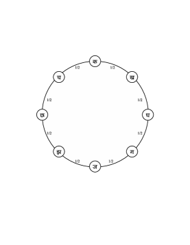
Figure 5: Weighted adjacency graph for noisy typewriter channel (2).

Figure 6: Weighted adjacency graph for noisy typewriter channel embedded in 3-dimensional hypercube. Thick lines represent edges that are used in the embedding. Dotted lines represent edges in the hypercube that are unused in the embedding.

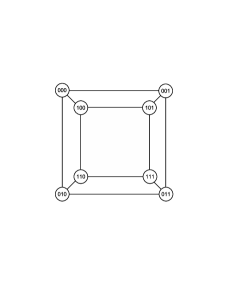
Figure 7: Hypercube graph labeled with binary reflected Gray code.

Clearly the error rate for this scheme is $\Delta=0$, since the code is lossless. Since all codewords are of length $3$, clearly $K=L=3$. To compute $M$, notice that any source symbol is perturbed to one of its neighbors with probability $1/2$. Further notice that the Hamming distance between neighbors in the hypercube is $1$. Thus $M=1/2$. We have seen that this encoding scheme achieves the entropy bounds $H(X)$ and $H(Y)$. It also achieves the $n=1$ lower bound for $M$ and is thus optimal for $n=1$. We can further drive $M$ down by increasing the block length. As shown in the following proposition, if a graph is embeddable in another graph and we take Cartesian products of each with itself, then the resulting graphs obey the same embedding relationship.

Definition 4

Consider two graphs $G$ and $H$ with vertices $V(G)$ and $V(H)$ and edges $E(G)$ and $E(H)$, respectively. Then $G$ is said to be embeddable into $H$ if $H$ has a subgraph isomorphic to $G$. That is, there is an injective map $\phi:V(G)\to V(H)$ such that $(u,v)\in E(G)$ implies $(\phi(u),\phi(v))\in E(H)$. This is denoted as $G\leadsto H$.

Definition 5

Consider two graphs $G_{1}$ and $G_{2}$ with vertices $V(G_{1})$ and $V(G_{2})$ and edges $E(G_{1})$ and $E(G_{2})$, respectively. Then the Cartesian product of $G_{1}$ and $G_{2}$, denoted $G_{1}\times G_{2}$ is a graph with vertex set $V(G_{1})\times V(G_{2})$ and for vertices $u=(u_{1},u_{2})$ and $v=(v_{1},v_{2})$, $(u,v)\in E(G_{1}\times G_{2})$ when ($u_{1}=v_{1}$ and $(u_{2},v_{2})\in E(G_{2})$) or ($u_{2}=v_{2}$ and $(u_{1},v_{1})\in E(G_{1})$).

Proposition 1

If $G_{1}\leadsto H_{1}$ and $G_{2}\leadsto H_{2}$, then $G_{1}\times G_{2}\leadsto H_{1}\times H_{2}$. A special case is that $G\leadsto H$ implies $G\times G\leadsto H\times H$.

Proof:

See Appendix B. ∎

Corollary 1

Let $G^{n}$ denote the $n$-fold Cartesian product of $G$ and $H^{n}$ the $n$-fold Cartesian product of $H$. If $G\leadsto H$, then $G^{n}\leadsto H^{n}$ for $n=1,2,\ldots$.

Proof:

By induction. ∎

Returning to our example, since the embedding relation is true for $n=1$, it is also true for $n=2,\ldots$, so we can embed $n$-fold Cartesian products of the adjacency graph into $n$-fold Cartesian products of the hypercube. Such a scheme would achieve rates of $K=3$ bits and $L=3$ bits. It would also achieve $M$ of $\tfrac{1}{n}\Pr[X_{1}^{n}\neq Y_{1}^{n}]$ since the Cartesian product of the adjacency graph represents exactly edit costs of $1$. For each $n$, this matches the lower bounds given in (1), and is thus optimal. Furthermore, asymptotically in $n$, the triple $(K,L,M)=(3,3,0)$ is achievable.

One may observe that embeddability into a graph where graph distance corresponds to edit distance seems to be sufficient to guarantee good performance; we will explore this in detail in the sequel. But first, we present a similar but more challenging situation as a contrast to the “best of all worlds” performance we have just seen.

With the source alphabet, representation alphabet, and distribution of $X$ remaining the same, let us suppose that the relationship between $X$ and $Y$ is given by

$$p(y|x)=\left[{\begin{array}[]{*{20}c}\tfrac{2}{5}&\tfrac{1}{5}&\tfrac{1}{20}&\tfrac{1}{5}&0&0&0&\tfrac{3}{20}\vspace{.5mm}\\ \tfrac{1}{5}&\tfrac{3}{5}&0&0&0&0&\tfrac{1}{5}&0\vspace{.5mm}\\ \tfrac{1}{20}&0&\tfrac{3}{5}&0&0&\tfrac{7}{20}&0&0\vspace{.5mm}\\ \tfrac{1}{5}&0&0&\tfrac{3}{5}&\tfrac{1}{5}&0&0&0\vspace{.5mm}\\ 0&0&0&\tfrac{1}{5}&\tfrac{3}{5}&0&0&\tfrac{1}{5}\vspace{.5mm}\\ 0&0&\tfrac{7}{20}&0&0&\tfrac{3}{5}&0&\tfrac{1}{20}\vspace{.5mm}\\ 0&\tfrac{1}{5}&0&0&0&0&\tfrac{3}{5}&\tfrac{1}{5}\vspace{.5mm}\\ \tfrac{3}{20}&0&0&0&\tfrac{1}{5}&\tfrac{1}{20}&\tfrac{1}{5}&\tfrac{2}{5}\vspace{.5mm}\\ \end{array}}\right]\mbox{.}$$ (3)

One can verify that, like (2), this is a stationary editing process. Thus, the rate bounds are unchanged at $K\geq 3$ and $L\geq 3$. Also, evaluation of (1) yields the bound $M\geq\frac{9}{20}$ for block size $n=1$. We will presently see that the three lower bounds cannot be achieved simultaneously, and we will determine the best values of $(K,L,M)$ for $n=1$.

The weighted adjacency graph corresponding to the new editing process is depicted in Fig. 8. Continuing to use the Hamming edit distance, to achieve $K=3$, $L=3$, and the $M$ lower bound simultaneously would require the embeddability of the graph of Fig. 8 into the hypercube of size $3$. Such embedding is clearly not possible since two nodes of the adjacency graph have degree $4$, whereas the maximum degree of the hypercube is $3$.

To achieve the least increase in $M$ above the lower bound (1), we must advantageously choose edges in the adjacency graph to break to create embeddability. (As we will see later, choosing the optimal set of edges to break involves solving the error-tolerant subgraph isomorphism problem.) In this example, the two nodes of degree $4$ must each have at least one edge broken. Picking the lowest weight edges (the two with weight $1/10$) is clearly the best choice, as the resulting graph can be embedded in the hypercube and cost of the edits k$\leftrightarrow$ G and c$\leftrightarrow$ J is increased by the least possible amount (from $1$ to $2$). Each of the broken edges has probability $\frac{1}{10}\cdot\frac{1}{8}$, so $M$ is increased above the previously computed minimum by $\frac{1}{40}$. Thus we achieve $(K,L,M)=(3,3,\frac{19}{40})$.

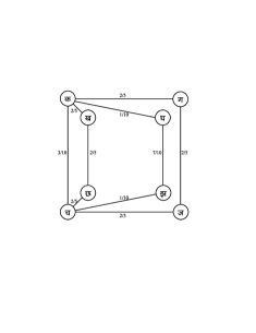
Figure 8: Weighted adjacency graph for stationary editing process (3).

We may alternatively aim for lower $M$ at the expense of $K$ and $L$. To determine whether the lower bound (1) can be achieved with $K=L=4$, we need to check if the weighted adjacency graph of Fig. 8 can be embedded in the hypercube of size $4$. Fig. 9 shows that this embedding is possible, with the code given in Table I. Thus one can achieve $(K,L,M)=(4,4,\frac{9}{20})$.

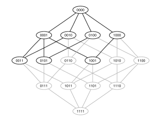
Figure 9: Weighted adjacency graph for editing process (3) embedded in 4-dimensional hypercube. Black lines represent edges that are used in the embedding. Gray lines represent edges in the hypercube that are unused in the embedding.

TABLE I: Code for the 4-dimensional hypercube embedding shown in Fig. 9.

k	$0000$	K	$0100$
G	$1000$	g	$0010$
j	$0011$	J	$1001$
C	$0101$	c	$0001$

VI-B Extension to Non-equiprobable Sources

The fact that both versions in the previous example were equiprobable and thus uncompressible might cast doubt on its gravity. Here we consider another example where the sources are not equiprobable. We will make use of variable-length lossless source codes and the Levenshtein distance as the edit distance. The basic edit operations are substitution, insertion, and deletion, as opposed to the Hamming distance where substitution is the only edit operation. Similar to the hypercube graph for the Hamming distance, we can create a Levenshtein edit distance graph. The Levenshtein graph of binary strings up to length $3$ is shown in Fig. 10.

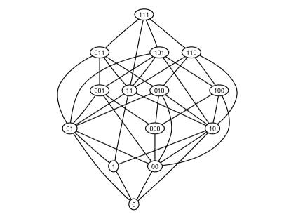
Figure 10: Levenshtein Edit Distance Graph for $\{0,1\}\cup\{0,1\}^{2}\cup\{0,1\}^{3}$.

Consider a memoryless source with alphabet $\mathcal{W}=\{$ k, K, G, g$\}$, with probabilities shown in Table II. Also in Table II, we find a Huffman code for the source, which is the best variable-length lossless source code [2]. Since the marginal distribution $p(x)$ is dyadic, it is at the center of a code attraction region of the binary Huffman code and achieves the entropy lower bound exactly [40]:

$$K=\sum\limits_{x\in\mathcal{W}}p(x)\ell(x)=1.75=H(X)=-\sum\limits_{x\in\mathcal{W}}p(x)\log_{2}p(x)\mbox{.}$$

TABLE II: Huffman Code for $4$-ary source.

$x\in\mathcal{W}$	$p(x)$	$f_{\mbox{Huffman}}(x)$	$\ell_{\mbox{Huffman}}(x)$	$p(x)\ell(x)$
k	$\tfrac{1}{2}$	$0$	$1$	$\tfrac{1}{2}$
K	$\tfrac{1}{4}$	$10$	$2$	$\tfrac{1}{2}$
G	$\tfrac{1}{8}$	$110$	$3$	$\tfrac{3}{8}$
g	$\tfrac{1}{8}$	$111$	$3$	$\tfrac{3}{8}$

Now consider a channel that is like the noisy typewriter channel, with channel transmission matrix

$$p(y|x)=\left[{\begin{array}[]{*{20}c}\tfrac{3}{4}&\tfrac{1}{2}&0&0\vspace{.5mm}\\ \tfrac{1}{4}&\tfrac{3}{8}&\tfrac{1}{4}&0\vspace{.5mm}\\ 0&\tfrac{1}{8}&\tfrac{1}{2}&\tfrac{1}{4}\vspace{.5mm}\\ 0&0&\tfrac{1}{4}&\tfrac{3}{4}\vspace{.5mm}\\ \end{array}}\right].$$ (4)

Evidently the editing is stationary, so the same Huffman code is optimal for both $X$ and $Y$. Constructing the adjacency graph yields Fig. 11.

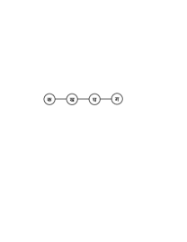
Figure 11: Adjacency graph for noisy typewriter-like channel.

This graph can be embedded (with matched vertex labels) in the Levenshtein graph using the Huffman assignment that we had developed, as shown in Fig. 12.

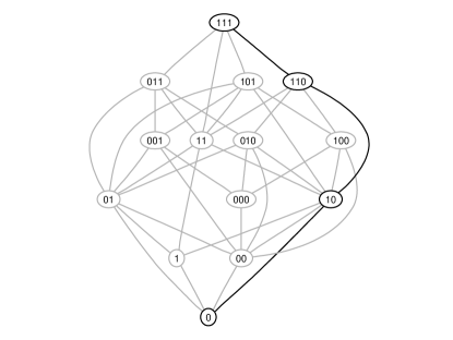
Figure 12: Adjacency graph for noisy typewriter-like channel embedded in the Levenshtein graph.

Evaluating the malleability lower bound (1) for $n=1$ in this case gives

$$M\geq\sum\limits_{x\in\mathcal{W}}\sum\limits_{y\in\mathcal{W}:y\neq x}p(x,y)=\tfrac{3}{8}\mbox{.}$$

With the code that we have used, we can achieve the triple $(K,L,M)=\left(\tfrac{7}{4},\tfrac{7}{4},\tfrac{3}{8}\right)$ which meets the $n=1$ lower bounds tightly, so it is optimal in the compression and malleability senses. As before, we can consider Cartesian products to reduce $M$, however, things are a bit more complicated since the Levenshtein graph does not grow as a Cartesian product.

VI-C Minimal Change Codes

As seen in the previous subsection, Gray codes and related minimal change code constructions seem to play a role in achieving good palimpsest performance. We review minimal change codes and some of their previous uses in communication theory, pointing out connections to our problem. We use minimal change codes to expand our treatment in the previous parts from using just Hamming or Levenshtein distances to include general edit distances.

Definition 6

Let $G$ be a connected graph. The path metric $d_{G}$ associated with the graph $G$ is the integer-valued metric on the vertices of $G$ which is defined by setting $d_{G}(u,v)$ equal to the length of the shortest path in $G$ joining $u$ and $v$.

Proposition 2

For any edit distance $d:\mathcal{V}^{*}\times\mathcal{V}^{*}\to[0,\infty)$, there exists a graph $G$ with vertex set $\mathcal{V}^{*}$ such that its path metric $d_{G}=d$.

Proof:

Construct a graph on vertex set $\mathcal{V}^{*}$ by adding an edge for any pair of vertices $A,B\in\mathcal{V}^{*}$ such that $d(A,B)=1$. ∎

Definition 7

An ordered codebook $(A_{i})$, $i=1,2,\ldots,|(A_{i})|$, $A_{i}\in\mathcal{V}^{*}$ is a minimal change code with respect to edit distance $d$ if it is a Hamiltonian path in a subgraph of the graph on $\mathcal{V}^{*}$ associated with $d$.

Our definition of minimal change codes is a generalization of Gray codes, which are Hamiltonian paths through the hypercube associated with Hamming distance [41]. Other minimal change codes may include Hamiltonian paths through the Levenshtein graph (Fig. 10), the de Bruijn graph, or the graph induced by Dobrushin’s distance functions for insertion/deletion channels [42]. There are countless other edit distances with numerous minimal change codes corresponding to each.

Minimal change codes have been used previously in the architecture design of parallel computers and in switching theory, among other places. Of particular interest to us, however, is their use in joint source-channel coding (JSCC) [43]. There are related problems in signal constellation labeling [39, 44, 45], in the genotype to phenotype mapping problem mentioned previously [22, 9], or in the problem of labeling books for ease of browsing [46]. There are also several theories of cognition based on preserving similarity relations from a source space in a representation space, though minimal change codes do not seem to be used explicitly [47].

Consider JSCC with source alphabet $\mathcal{X}$, channel input alphabet $\mathcal{A}$, channel output alphabet $\mathcal{B}$, and source reconstruction alphabet $\mathcal{Y}$. Then the injective mapping between $\mathcal{X}$ and $\mathcal{A}$ is the index assignment for JSCC. The mapping between $\mathcal{A}$ and $\mathcal{B}$ is given by the noisy channel, a transition probability assignment, $p(b|a)$. The surjective mapping between $\mathcal{B}$ and $\mathcal{Y}$ is the inverse index assignment operation. The goal in selecting index assignments is to minimize the distortion between the $\mathcal{X}-\mathcal{Y}$ spaces when there are errors between the $\mathcal{A}-\mathcal{B}$ spaces. Informally using terminology from genetics, the source spaces $\mathcal{X}$ and $\mathcal{Y}$ are cast as phenotype, whereas the index spaces $\mathcal{A}$ and $\mathcal{B}$ are cast as genotype. Then index assignment aims to have small mutations in genotype result in small changes in phenotype.

In the palimpsest problem, the injective and surjective mappings between $\mathcal{X}$ and $\mathcal{A}$ as well as $\mathcal{B}$ and $\mathcal{Y}$ are basically the same as in the joint source channel coding problem. The distinction between the two problems is that for malleable coding, there is a transition probability assignment between $\mathcal{X}$ and $\mathcal{Y}$, rather than between $\mathcal{A}$ and $\mathcal{B}$. One goal is to minimize the distance between words in the $\mathcal{A}$ and $\mathcal{B}$ spaces for perturbations in the $\mathcal{X}$ and $\mathcal{Y}$ spaces. Using the genetics analogy, index assignments so that small changes in phenotype result in small changes in genotype are desired. One might even call malleable coding a problem in joint channel source coding.

Considering that index assignment for JSCC, signal constellation labeling, and the palimpsest problem are so similar, it is not surprising that Gray codes come up in all of them [43, 39]. All are essentially problems of embedding: performing a transformation on objects of one type to produce objects of a new type such that the distance between the transformed objects approximates the distance between the original objects [25].

VII General Characterizations

We have seen that there may be a trade-off between the various parameters $(K,L,M)$ and have found several easily achieved points. Our interest now turns to obtaining more detailed characterizations of $\mathfrak{P}_{V}$ and $\mathfrak{P}_{B}$, the sets of achievable rate–malleability triples.

VII-A Variable-length Coding

We begin with characterization of $\mathfrak{P}_{V}$, which is a problem in zero error information theory [48, 49]. Our results are expressed in terms of the solution to an error-tolerant attributed subgraph isomorphism problem [5], which we first describe in general.

VII-A1 Error-Tolerant Attributed Subgraph Isomorphism Problem

A vertex-attributed graph is a three-tuple $G=(V,E,\mu)$, where $V$ is the set of vertices, $E\subseteq V\times V$ is the set of edges, and $\mu:V\to\mathcal{V}^{*}$ is a function assigning labels to vertices. The set of labels is denoted $\mathcal{V}^{*}$. The definition of embedding for attributed graphs has a slightly stronger requirement than for unattributed graphs, Def. 4.

Definition 8

Consider two vertex-attributed graphs $G=(V(G),E(G),\mu_{G})$ and $H=(V(H),E(H),\mu_{H})$. Then $G$ is said to be embeddable into $H$ if $H$ has a subgraph isomorphic to $G$. That is, there is an injective map $\phi:V(G)\to V(H)$ such that $\mu_{G}(v)=\mu_{H}(\phi(v))$ for all $v\in V(G)$ and that $(u,v)\in E(G)$ implies $(\phi(u),\phi(v))\in E(H)$. This is denoted as $G\leadsto H$.

Several graph editing operations may be defined, such as substituting a vertex label, deleting a vertex, deleting an edge, and inserting an edge. These four operations are powerful enough to transform any attributed graph into a subgraph of any other attributed graph. The edited graph is denoted through the operator $\mathcal{E}(\cdot)$ corresponding to the sequence of graph edit operations $\mathcal{E}=(e_{1},\ldots,e_{k})$. There is a cost associated with each sequence of graph edit operations, $C(\mathcal{E})$.

Definition 9

Given two graphs $G$ and $H$, an error-correcting attributed subgraph isomorphism $\psi$ from $G$ to $H$ is the composition of two operations $\psi=(\mathcal{E},\phi_{\mathcal{E}})$ where

• $\mathcal{E}$ is a sequence of graph edit operations such that there exists a $\mathcal{E}(G)$ that satisfies $\mathcal{E}(G)\leadsto H$.

• $\phi_{\mathcal{E}}$ is an embedding of $\mathcal{E}(G)$ into $H$.

Definition 10

The subgraph distance $\rho(G,H)$ is the cost of the minimum cost error-correcting attributed subgraph isomorphism $\psi$ from $G$ to $H$.

Note that in general, $\rho(G,H)\neq\rho(H,G)$.

Remark 1

It should be noted that the subgraph isomorphism problem is NP-complete [50], and therefore the error-tolerant subgraph isomorphism problem is in the class NP and is generally harder than the exact subgraph isomorphism problem [5].

VII-A2 Closeness Vitality

The subgraph isomorphism cost structure for the palimpsest problem is based on a graph theoretic quantity called the closeness vitality [51]. Vitality measures determine the importance of particular edges and vertices in a graph.

Definition 11

Let $\mathfrak{G}$ be the set of all graphs $G=(V,E)$, and let $f:\mathfrak{G}\to\mathbb{R}$ be any real-valued function on $\mathfrak{G}$. A vitality index $v(G,x)$ is the difference of the values of $f$ on $G$ and on $G$ without element $x$; it satisfies $v(G,x)=f(G)-f(G-x)$.

A particular vitality index is the closeness vitality, defined in terms of the Wiener index [52], which is simply the sum of all pairwise distances.

Definition 12

The Wiener index $f_{W}(G)$ of a graph $G$ is the sum of the distances of all vertex pairs:

$$f_{W}(G)=\sum_{v\in V}\sum_{w\in V}d(v,w)\mbox{.}$$

Definition 13

The closeness vitality $\operatorname{cv}(G,x)$ is the vitality index with respect to the Wiener index:

$$\operatorname{cv}(G,x)=f_{W}(G)-f_{W}(G-x)\mbox{.}$$

In addition to the application in the palimpsest problem, the closeness vitality also determines traffic-related costs in all-to-all routing networks.

Finding the distance matrix to compute the Wiener index involves solving the all-pairs shortest path problem. Finding the distance matrix of a modified graph from the distance matrix of the original graph involves solving the dynamic all-pairs shortest path problem [53, 54].

VII-A3 $\mathfrak{P}_{V}$ Characterization

For our purposes, we are concerned with the error-tolerant embedding of an attributed, weighted source adjacency graph into the graph induced by a $\mathcal{V}^{*}$-space edit distance. As such, edge deletion will be the only graph editing operation that is required. Error-tolerant embedding problems in pattern recognition and machine vision often have simple cost functions [5, 55]; our cost function is determined by the closeness vitality and is not so simple.

To characterize $\mathfrak{P}_{V}$, let us first consider the delay-free case, $n=1$. A source $p(X,Y)$ and an edit distance $d(\cdot,\cdot)$ are given. It is known [2] that Huffman coding provides the minimal redundancy instantaneous code and achieves expected performance $H(X)\leq K\leq H(X)+1$. Similarly, a Huffman code for $Y$ would yield $H(Y)\leq L\leq H(Y)+1$. The rate loss for using an incorrect Huffman code is essentially as given in Fig. 4. Suppose that we require that the rate lower bound is met, i.e. we must use a Huffman code for some $Z$ that is on the geodesic between $X$ and $Y$. This code will satisfy the Kraft inequality [56]. Note that for a given $Z$, there are several Huffman codes: those arising from different labelings of the code tree and also perhaps different trees [57]. Let us denote the set of all Huffman codes for $Z$ as $\mathcal{H}_{Z}$.

Since $K$ and $L$ are fixed by the choice of $Z$, all that remains is to determine the set of achievable $M$. Let $G$ be the graph induced by the edit distance $d(\cdot,\cdot)$, and $d_{G}$ its path metric. The graph $G$ is intrinsically labeled. Let $A$ be the weighted adjacency graph of the source $p(X,Y)$, with vertices $\mathcal{W}$, edges $E(A)$ a subset of $\mathcal{W}\times\mathcal{W}$, and labels given by a Huffman code. That is $A=(\mathcal{W},E(A),f_{E})$ for some $f_{E}\in\mathcal{H}_{Z}$. There is a path semimetric, $d_{A}$, associated with the graph $A$ (since the adjacency graph is weighted, it might not satisfy the triangle inequality).

As may be surmised from Section V, the basic problem is to solve the error-tolerant subgraph isomorphism problem of embedding $A$ into $G$. In general for $n=1$, the malleability cost under edit distance $d_{G}$ when using the source code $f_{E}$ is

$$M=\sum_{x\in\mathcal{W}}\sum_{y\in\mathcal{W}}p(x,y)d_{G}(f_{E}(x),f_{E}(y))\mbox{.}$$

The smallest malleability possible is when $A=(\mathcal{W},E(A),f_{E})$ is a subgraph of $G$, and then

$$M_{min}=\sum_{x\in\mathcal{W}}\sum_{y\in\mathcal{W}}p(x,y)d_{A}(x,y)=\sum_{x\in\mathcal{W}}\sum_{y\in\mathcal{W}}p(x,y)d_{G}(f_{E}(x),f_{E}(y))=\Pr[X\neq Y]\mbox{,}$$

which is simply the expected Wiener index

$$M_{min}=E[f_{W}(A)]=\Pr[X\neq Y]\mbox{.}$$

If edges in $A$ need to broken in order to make it a subgraph of $G$, then $M$ increases as a result. The cost of graph editing operations in the error-tolerant embedding problem should reflect the effect on $M$. If an edge $\bar{e}$ is removed from the graph $A$, the resulting graph is called $A-\bar{e}$; it induces its own path semimetric $d_{A-\bar{e}}$. Thus the cost of removing an edge, $\bar{e}$, from the graph $A$ is given by the following expression as a function of the associated removal operation $e$:

$$C(e)=\sum_{x\in\mathcal{W}}\sum_{y\in\mathcal{W}}p(x,y)\left[d_{A-\bar{e}}(f_{E}(x),f_{E}(y))-d_{A}(f_{E}(x),f_{E}(y))\right]\mbox{,}$$

which is the negative expected closeness vitality

$$C(\delta)=-E[\operatorname{cv}(A,e)].$$

If $\mathcal{E}$ is a sequence of edge removals, $\bar{\mathcal{E}}$, then

$$C(\mathcal{E})=\sum_{x\in\mathcal{W}}\sum_{y\in\mathcal{W}}p(x,y)\left[d_{A-\bar{\mathcal{E}}}(f_{E}(x),f_{E}(y))-d_{A}(f_{E}(x),f_{E}(y))\right]\mbox{,}$$

which is

$$C(\mathcal{E})=-E[\operatorname{cv}(A,\bar{\mathcal{E}})]\mbox{.}$$

As seen, the cost function is quite different from standard error-tolerant embedding problems [5, 55] since it depends not only on which edge is broken, but also on the remainder of the graph.

Putting things together, we see that $\mathfrak{P}_{V}$ contains any point

$$(K,L,M)=\left(H(X)+D(p_{X}\|p_{Z})+1,H(Y)+D(p_{Y}\|p_{Z})+1,M_{min}+\mathop{\min}\limits_{f_{E}\in\mathcal{H}_{Z}}\rho(A,G)\right)\mbox{.}$$

The previous analysis had assumed $n=1$. We may increase the block length and improve performance.

Theorem 1

Consider a source $p(X,Y)$ with associated (unlabeled) weighted adjacency graph $A$ and an edit distance $d$ with associated graph $G$. For any $n$, let $\mathfrak{P}_{V}^{(ach)}$ be the set of triples $(K,L,M)$ that are computed, by allowing an arbitrary choice of the memoryless random variable $p(Z_{1}^{n})$, as follows:

$$K=H(X)+D(p_{X}\|p_{Z})+\tfrac{1}{n}\mbox{,}$$

$$L=H(Y)+D(p_{Y}\|p_{Z})+\tfrac{1}{n}\mbox{,}$$

$$M=\tfrac{1}{n}\Pr[X_{1}^{n}\neq Y_{1}^{n}]+\tfrac{1}{n}\mathop{\min}\limits_{f_{E}\in\mathcal{H}_{Z_{1}^{n}}}\rho(A=(\mathcal{W}^{n},E(A),f_{E}),G)\mbox{.}$$

Then the set of triples $\mathfrak{P}_{V}^{(ach)}\subseteq\mathfrak{P}_{V}$ is achievable instantaneously.

Proof:

A non-degenerate random variable $Z_{1}^{n}$ is fixed. There is a family of instantaneous lossless codes (with $\Delta=0$) that corresponds to this random variable, denoted $\{(f_{E},f_{D})\}=\mathcal{H}_{Z_{1}^{n}}$, through the McMillan sum. By the results in [26], any of these codes achieve rates $K\leq H(X)+D(p_{X}\|p_{Z})+\tfrac{1}{n}$ and $L\leq H(Y)+D(p_{Y}\|p_{Z})+\tfrac{1}{n}$. Moreover, by the graph embedding construction, a code $(f_{E},f_{D})$ achieves $M=\tfrac{1}{n}\Pr[X_{1}^{n}\neq Y_{1}^{n}]+\tfrac{1}{n}\rho(A=(\mathcal{W}^{n},E(A),f_{E}),G)$. Since all codes in $\mathcal{H}_{Z_{1}^{n}}$ have the same rate performance, a code in the family that minimizes $\rho$ may be chosen. ∎

The above theorem states that error-tolerant subgraph isomorphism implies achievable malleability. The choice of the auxiliary random variable $Z$ is open to optimization. If minimal rates are desired, then $p_{Z}$ should be on the geodesic connecting $p_{X}$ and $p_{Y}$. If $Z$ is not on the geodesic, then there is some rate loss, but perhaps there can be some malleability gains.

Note that when $p(y|x)$ is a stationary editing process, there is the possibility of the simple lower bounds being tight to this achievable region.

Corollary 2

Consider a source as given above in Theorem 1. If $p(y|x)$ is stationary, $p(x)=p(y)$ is $|\mathcal{V}|$-adic, and there is a Huffman-labeled $A$ for $p(x)=p(y)$ that is an isometric subgraph of $G$, then the block length $n$ lower bound $(H(X),H(Y),\tfrac{1}{n}\Pr[X_{1}^{n}\neq Y_{1}^{n}])$ is tight to this achievable region for every $n$, and in particular to $(H(X),H(Y),0)$ for large $n$.

VII-B Block Coding

Now we turn our attention to the block-coding palimpsest problem. For $\mathfrak{P}_{B}$, we use a joint typicality graph rather than the weighted adjacency graph used for $\mathfrak{P}_{V}$. Additionally we focus on binary block codes under Hamming edit distance, so we are concerned only with hypercubes rather than general edit distance graphs.

We can use graph-theoretic ideas to formally state an achievability result for the block coding palimpsest problem. As shown in the constructive examples above, there are schemes for which an improvement on $M$ may be achieved by increasing $L$. However, the resulting compression of $Y_{1}^{n}$ is not unique, and thus is not optimal. We wish to expurgate the redundant representations of $Y_{1}^{n}$ as efficiently as possible, by the aid of a graph. However, in doing so, we have to also consider the representations and how they are related to one another. First we review some standard typicality arguments (from [58]) and then define a graph from typical sets.

Definition 14

The strongly typical set $T^{n}_{[X]\delta}$ with respect to $p(x)$ is

$$T^{n}_{[X]\delta}=\left\{x_{1}^{n}\in\mathcal{X}^{n}\mid\sum_{x}\left|\tfrac{1}{n}N(x;x_{1}^{n})-p(x)\right|\leq\delta\right\}\mbox{,}$$

where $N(x;x_{1}^{n})$ is the number of occurrences of $x$ in $x_{1}^{n}$ and $\delta>0$.

Definition 15

The strongly jointly typical set $T^{n}_{[XY]\delta}$ with respect to $p(x,y)$ is

$$T^{n}_{[XY]\delta}=\left\{(x_{1}^{n},y_{1}^{n})\in\mathcal{X}^{n}\times\mathcal{Y}^{n}\mid\sum_{x}\sum_{y}\left|\tfrac{1}{n}N(x,y;x_{1}^{n},y_{1}^{n})-p(x,y)\right|\leq\delta\right\}\mbox{.}$$

Definition 16

For any $x_{1}^{n}\in T^{n}_{[X]\delta}$, define a strongly conditionally typical set

$$T^{n}_{[Y|X]\delta}(x_{1}^{n})=\left\{y_{1}^{n}\in T^{n}_{[Y]\delta}\mid(x_{1}^{n},y_{1}^{n})\in T^{n}_{[XY]\delta}\right\}\mbox{.}$$

Definition 17

Let the connected strongly typical set be

$$S^{n}_{[X]\delta}=\left\{x_{1}^{n}\in T^{n}_{[X]\delta}\mid T^{n}_{[Y|X]\delta}(x_{1}^{n})\mbox{ is nonempty}\right\}\mbox{.}$$

Now that we have definitions of typical sets, we put forth some lemmas.

Lemma 1 (Strong AEP)

Let $\eta$ be a small positive number such that $\eta\to 0$ as $\delta\to 0$. Then for sufficiently large $n$,

$$\left|T^{n}_{[X]\delta}\right|\leq 2^{n(H(X)+\eta)}\mbox{.}$$

Proof:

See [58, Theorem 5.2]. ∎

Lemma 2 (Strong JAEP)

Let $\lambda$ be a small positive number such that $\lambda\to 0$ as $\delta\to 0$. Then for sufficiently large $n$,

$$\Pr[(X_{1}^{n},Y_{1}^{n})\in T^{n}_{[XY]\delta}]>1-\delta$$

and

$$(1-\delta)2^{n(H(X,Y)-\lambda)}\leq\left|T^{n}_{[XY]\delta}\right|\leq 2^{n(H(X,Y)+\lambda)}\mbox{.}$$

Proof:

See [58, Theorem 5.8]. ∎

Lemma 3

If $\delta(n)$ satisfies the following conditions, then Lemma 2 remains valid:

$$\delta(n)\to 0\mbox{ and }\sqrt{n}\delta(n)\to\infty\mbox{ as }n\to\infty\mbox{.}$$

Proof:

See [59, (2.9) on p. 34]. ∎

Lemma 4

If $\left|T^{n}_{[Y|X]\delta}(x_{1}^{n})\right|\geq 1$, then

$$2^{n(H(Y|X)-\nu)}\leq\left|T^{n}_{[Y|X]\delta}(x_{1}^{n})\right|\leq 2^{n(H(Y|X)+\nu)}\mbox{,}$$

where $\nu\to 0$ as $n\to\infty$ and $\delta\to 0$.

Proof:

See [58, Theorem 5.9]. ∎

Lemma 5

$$(1-\delta)2^{n(H(X)-\psi)}\leq\left|S^{n}_{[X]\delta}\right|\leq 2^{n(H(X)+\psi)}\mbox{,}$$

where $\psi\to 0$ as $n\to\infty$ and $\delta\to 0$. Also, for any $\delta>0$,

$$\Pr[X_{1}^{n}\in S^{n}_{[X]\delta}]>1-\delta$$

for $n$ sufficiently large.

Proof:

See [58, Corollary 5.11], Lemma 1, and [58, Proposition 5.12]. ∎

For the bivariate distribution $p(x,y)$, define a square matrix called the strong joint typicality matrix $A^{n}_{[XY]}$ as follows. There is one row (and column) for each sequence in $S^{n}_{[X]\delta}\cup S^{n}_{[Y]\delta}$. The entry with row corresponding to $x_{1}^{n}$ and column corresponding to $y_{1}^{n}$ receives a one if $(x_{1}^{n},y_{1}^{n})$ is strongly jointly typical and zero otherwise.

VII-B1 Stationary Editing

Now let us restrict ourselves to the class of bivariate distributions with equal marginals:

$$\mathcal{P}=\left\{p(x,y)\mid p(x)=p(y)\right\}\mbox{,}$$

which is the class of distributions with stationary editing. In this class, we avoid the mismatch redundancy and also reduce the number of performance parameters from 3 to 2. After this restriction, it is clear that the $x$-typical set and the $y$-typical set coincide. Moreover, $H(X)=H(Y)$ and $H(Y|X)=H(X|Y)=H(X)-I(X;Y)$. Thus it follows that asymptotically, $A^{n}_{[XY]}$ will be a square matrix with an approximately equal number of ones in all columns and in all rows. Think of $A^{n}_{[XY]}$ as the adjacency matrix of a graph, where the vertices are sequences and edges connect sequences that are jointly typical with one another.

Proposition 3

Take $A^{n}_{[XY]}$ for some source in $\mathcal{P}$ as the adjacency matrix of a graph $\mathcal{G}^{n}$. The number of vertices in the graph will satisfy

$$(1-\delta)2^{n(H(X)-\psi)}\leq\left|V(\mathcal{G}^{n})\right|\leq 2^{n(H(X)+\psi)}\mbox{,}$$

where $\psi\to 0$ as $n\to\infty$ and $\delta\to 0$. The degree of each vertex, $\mbox{deg}_{v}$, will concentrate as

$$2^{n(H(Y|X)-\nu)}\leq\mbox{deg}_{v}\leq 2^{n(H(Y|X)+\nu)}\mbox{,}$$

where $\nu\to 0$ as $n\to\infty$ and $\delta\to 0$.

Proof:

Follows from the previous lemmas. ∎

Having established the basic topology of the strongly typical set as asymptotically a $2^{nH(Y|X)}$-regular graph on $2^{nH(X)}$ vertices, we return to the coding problem. Using graph embedding ideas yields a theorem on block palimpsest achievability.

Theorem 2

For a source $p(x,y)\in\mathcal{P}$ and the Hamming edit distance, a triple $(K,K,M=M_{min})$ is achievable if $\mathcal{G}^{n}\leadsto H_{nK}$.

Proof:

To achieve $M_{min}$, we need to assign binary codewords to each of the $2^{nH(X)}$ vertices, such that the Hamming distance between the codeword of a vertex and the codewords of any of its neighbors is $1$. Using the binary reflected Gray code of length $nK$ and the hypercube that it induces, the construction reduces to finding an embedding of $\mathcal{G}^{n}$ into the hypercube of size $nK$, denoted $H_{nK}$. Thus a sufficient condition for block-code achievability, while requiring $M=M_{min}$, is $\mathcal{G}^{n}\leadsto H_{nK}$. ∎

Using this result, we argue that a linear increase in malleability is at exponential cost in code length. By a simple counting argument, we present a condition for embeddability.

Theorem 3

For a source $p(x,y)\in\mathcal{P}$ and the Hamming edit distance, asymptotically, if $\mathcal{G}^{n}\leadsto H_{nK}$ then

$$nK\geq\max\left(nH(X),2^{nH(Y|X)}\right)\mbox{.}$$ (5)

Proof:

The hypercube $H_{nK}$ is an $nK$-regular graph with $2^{nK}$ vertices. As a minimal condition for embeddability, the number of vertices in the hypercube must be greater than or equal to the number of vertices in the graph to be embedded, i.e. $nK\geq n(H(X)+\psi)$. As another minimal condition for embeddability, the degree of the hypercube must be greater than or equal to the maximal degree of the graph to be embedded, so $nK\geq 2^{n(H(Y|X)+\nu)}$. Combining the two conditions and letting $\psi\to 0$ and $\nu\to 0$ as $n\to\infty$ yields the desired result. ∎

This theorem is one of our main results. It should be noted that even if we allowed some asymptotically small slack in breaking some edges to perform embedding, i.e. we solved an error-tolerant subgraph isomorphism problem with error tolerance $\xi$, this would not help, since we would need to break a constant fraction of edges in $\mathcal{G}^{n}$ to reduce the maximal degree. In particular, since each of the $nH(X)$ vertices in $\mathcal{G}^{n}$ asymptotically has the same degree, to reduce the maximal degree even by one would require breaking $\xi\geq nH(X)$ edges. Clearly $\xi\nrightarrow 0$ as $n\to\infty$.

This result can be interpreted as follows. When using binary codes that achieve the minimal malleability parameter, the length of the code must be greater than $\max\left(nH(X),2^{nH(Y|X)}\right)$. If $2^{nH(Y|X)}$ is much greater than $nH(X)$, i.e. the two versions are not particularly well correlated, this implies that to achieve minimal malleability requires a significant length expansion of the codewords over the entropy bound. Taking this to an extreme, suppose that $X$ and $Y$ are independent. Then $2^{nH(Y|X)}=2^{nH(X)}$, and an exponential expansion is required, just as in the universal PPM scheme of Section V-D.

If we want to understand the embeddability requirements further, we would need to understand the topology of $\mathcal{G}^{n}$ further. Just knowing that it is asymptotically regular does not seem to be enough. Several properties that are equivalent to exact hypercube embeddability are given in [60, 61]. Of course we can break some small fraction $\xi$ of edges in the graph to satisfy the embeddability conditions as long as $\xi\to 0$ as $n\to\infty$. If we no longer require that $nM$ be the minimal possible, then we are back to the same kind of error-tolerant subgraph isomorphism formulation given for variable length coding in the previous section. The only change in the characterization of the achievable region is that rather than restricting the encoder to be the Huffman code of an auxiliary random variable $Z_{1}^{n}$, here one would need to test the error-tolerant subgraph isomorphism functional over all permutations of labelings.

VII-B2 General Editing

If we remove our restriction of $p(x,y)\in\mathcal{P}$, then we can create $A^{n}_{[XY]}$ as before. While the resulting graph would not be asymptotically regular, the basic result on paying an exponential rate penalty will still hold.

The space $S^{n}\triangleq S^{n}_{[X]\delta}\cup S^{n}_{[Y]\delta}$ with the corresponding path metric, $d_{A}$ induced by $A^{n}_{[XY]}$ is a metric space. Hypercubes with their natural path metric, $d_{G}$, are also a metric space. Rather than requiring absolutely minimal $nM$, it can be noted that $M$ is asymptotically zero when the Lipschitz constant associated with the mapping between the source space and the representation space has nice properties in $n$.

Definition 18

A mapping $f$ from the metric space $(S^{n},d_{A^{n}})$ to the metric space $(\mathcal{V}^{nK},d_{G^{n}})$ is called Lipschitz continuous if

$$d_{G^{n}}(f(x_{1}),f(x_{2}))\leq Cd_{A^{n}}(x_{1},x_{2})$$

for some constant $C$ and for all $x_{1},x_{2}\in S^{n}$. The smallest such $C$ is the Lipschitz constant:

$$\operatorname{Lip}[f]=\sup\limits_{x_{1}\neq x_{2}\in S^{n}}\frac{d_{G^{n}}\left(f(x_{1}),f(x_{2})\right)}{d_{A^{n}}(x_{1},x_{2})}\mbox{.}$$

The Lipschitz constant is also called the dilation of an embedding, since it is the maximum amount that any edge in $\mathcal{G}^{n}$ is stretched as it is replaced by a path in $H_{nK}$ [62, 63]. A related quantity is the Lipschitz constant of the inverse mapping, called the contraction:

$$\operatorname{Lip}[f^{-1}]=\sup\limits_{x_{1}\neq x_{2}\in S^{n}}\frac{d_{A^{n}}(x_{1},x_{2})}{d_{G^{n}}\left(f(x_{1}),f(x_{2})\right)}\mbox{.}$$

The product of the dilation and contraction $\operatorname{Lip}[f]\operatorname{Lip}[f^{-1}]$ is called the distortion. Another property of metric embeddings in the expansion, which is the ratio of the sizes of the two finite metric spaces,

$$\operatorname{expan}[f]=\frac{|\mathcal{V}^{nK}|}{|S^{n}|}\mbox{.}$$

We can bound the malleability $M$, for a coding scheme that only represents sequences in $S^{n}$ as follows.

Theorem 4

Let the Lipschitz constant be as defined. Then for a coding scheme $f_{E}$ that only represents sequences in $S^{n}=S^{n}_{[X]\delta}\cup S^{n}_{[Y]\delta}$, we have that

$$M\leq\frac{\operatorname{Lip}[f_{E}]}{n}\left(1+\delta\operatorname{diam}(\mathcal{G}^{n})\right)$$

Proof:

The proof is given as follows:

$$M =\frac{1}{n}\sum\limits_{x_{1}^{n}\in S^{n}}\sum\limits_{y_{1}^{n}\in S^{n}}p(x_{1}^{n},y_{1}^{n})d_{G^{n}}(f_{E}(x_{1}^{n}),f_{E}(y_{1}^{n}))$$

$$\stackrel{{\scriptstyle(a)}}{{\leq}}\frac{1}{n}\sum\limits_{x_{1}^{n}\in S^{n}}\sum\limits_{y_{1}^{n}\in S^{n}}p(x_{1}^{n},y_{1}^{n})\operatorname{Lip}[f_{E}]d_{A^{n}}(x_{1}^{n},y_{1}^{n})$$

$$=\frac{\operatorname{Lip}[f_{E}]}{n}\sum\limits_{x_{1}^{n}\in S^{n}}\sum\limits_{y_{1}^{n}\in S^{n}}p(x_{1}^{n},y_{1}^{n})d_{A^{n}}(x_{1}^{n},y_{1}^{n})$$

$$=\frac{\operatorname{Lip}[f_{E}]}{n}\left\{\sum\limits_{\begin{subarray}{c}x_{1}^{n}\in S^{n},y_{1}^{n}\in S^{n}\\ (x_{1}^{n},y_{1}^{n})\in T^{n}_{[XY]\delta}\end{subarray}}p(x_{1}^{n},y_{1}^{n})d_{A^{n}}(x_{1}^{n},y_{1}^{n})+\sum\limits_{\begin{subarray}{c}x_{1}^{n}\in S^{n},y_{1}^{n}\in S^{n}\\ (x_{1}^{n},y_{1}^{n})\notin T^{n}_{[XY]\delta}\end{subarray}}p(x_{1}^{n},y_{1}^{n})d_{A^{n}}(x_{1}^{n},y_{1}^{n})\right\}$$

$$\stackrel{{\scriptstyle(b)}}{{=}}\frac{\operatorname{Lip}[f_{E}]}{n}\left\{\Pr\left[(x_{1}^{n},y_{1}^{n})\in T^{n}_{[XY]\delta}\right]+\sum\limits_{\begin{subarray}{c}x_{1}^{n}\in S^{n},y_{1}^{n}\in S^{n}\\ (x_{1}^{n},y_{1}^{n})\notin T^{n}_{[XY]\delta}\end{subarray}}p(x_{1}^{n},y_{1}^{n})d_{A^{n}}(x_{1}^{n},y_{1}^{n})\right\}$$

$$\stackrel{{\scriptstyle(c)}}{{\leq}}\frac{\operatorname{Lip}[f_{E}]}{n}\left\{1+\delta\max\limits_{\begin{subarray}{c}x_{1}^{n}\in S^{n},y_{1}^{n}\in S^{n}\\ (x_{1}^{n},y_{1}^{n})\notin T^{n}_{[XY]\delta}\end{subarray}}d_{A^{n}}(x_{1}^{n},y_{1}^{n})\right\}$$

$$=\frac{\operatorname{Lip}[f_{E}]}{n}\left\{1+\delta\operatorname{diam}(\mathcal{G}^{n})\right\}\mbox{,}$$

where step (a) is by definition of the Lipschitz constant; step (b) follows from the definition of graph distance and the consistency of strong typicality ([58, Theorem 5.7]); and step (c) is from bounding $\Pr\left[(x_{1}^{n},y_{1}^{n})\in T^{n}_{[XY]\delta}\right]$ by $1$ and from Lemma 2. Note that the $\delta$ bound used in step (c) for the probability of sequences pairs that are both marginally typical but not jointly typical is actually the probability of all non-jointly typical pairs and is therefore loose. ∎

Computing Lipschitz constants is usually difficult or impossible. There are, however, methods from theoretical computer science for bounding Lipschitz constants (or dilation) for embeddings [62, 63]. For a “host” graph $\mathcal{H}$ and a “guest” graph $\mathcal{G}$, a basic counting argument reminiscent of Theorem 3, shows that the dilation for any embedding of $\mathcal{G}$ into $\mathcal{H}$ must satisfy

$$\operatorname{Lip}[f_{E}]\geq\left\lceil\frac{\log(d_{\mathcal{G}}-1)}{\log(d_{\mathcal{H}}-1)}\right\rceil\mbox{,}$$

where $d_{\mathcal{G}}$ and $d_{\mathcal{H}}$ are the respective maximum degrees [62, Prop. 1.5.2]. When the guest graph is the joint typicality graph $\mathcal{G}^{n}$ and the host graph is the hypercube $H_{nK}$, this implies that

$$\operatorname{Lip}[f_{E}]\geq\left\lceil\frac{\log(2^{n(H(Y|X)+\nu)}-1)}{\log(nK-1)}\right\rceil\approx\frac{nH(Y|X)}{\log nK}\mbox{.}$$

Another typical result arises when it is fixed that both graphs have $m$ vertices (expansion is $1$). The Lipschitz constant bound is in terms the bisection width $W_{\mathcal{G}}$ and the recursive edge-bisector function $R_{\mathcal{H}}(\cdot)$. The dilation $\operatorname{Lip}[f_{E}]$ of any embedding $f_{E}$ of $\mathcal{G}$ into $\mathcal{H}$ must satisfy

$$\operatorname{Lip}[f_{E}]\geq\left(\frac{1}{\log d_{\mathcal{H}}}\right)\log\frac{W_{\mathcal{G}}}{d_{\mathcal{G}}R_{\mathcal{H}}(m)}-1\mbox{.}$$

The bisection width of a graph is the size of the smallest cut-set that breaks the graph into two subgraphs of equal sizes (to within rounding) [62, Prop. 2.3.6]. Using such a result is difficult since the bisection width of the joint typicality graph is not known. For the case when $\mathcal{H}=H_{\lceil nH(X)\rceil}$, a simplified version reduces to

$$\operatorname{Lip}[f_{E}]\geq\frac{\lceil\log m\rceil}{\operatorname{diam}(\mathcal{G}^{n})}\approx\frac{nH(X)}{\operatorname{diam}(\mathcal{G}^{n})}\mbox{,}$$

where $\operatorname{diam}(\mathcal{G}^{n})$ is the same graph diameter we had seen before [63]. If the dilation is to be no greater than $2$, the PPM scheme we have described previously may be reinterpreted in a graph embedding framework and seen to achieve $\operatorname{Lip}[f_{E}]\leq 2$, but the price is exponential expansion, $\operatorname{expan}[f_{E}]=\frac{1}{m}{2^{m-1}}$.

Returning to Theorem 4, as noted in Lemma 3, $\delta$ can be taken as

$$\delta(n)=n^{-\frac{1}{2}+\omega}$$

for some fixed $\omega>0$. The diameter of the hypercube $H_{nK}$ is clearly $nK$. Combining this with the contraction provides a bound on the diameter of $\mathcal{G}^{n}$:

$$\operatorname{diam}(\mathcal{G}^{n})\leq\operatorname{Lip}[f_{E}^{-1}]nK\mbox{.}$$

Thus one can further bound the expression in Theorem 4 as

$$M \leq\frac{\operatorname{Lip}[f_{E}]}{n}\left(1+\delta\operatorname{diam}(\mathcal{G}^{n})\right)$$

$$\leq\frac{\operatorname{Lip}[f_{E}]}{n}\left(1+n^{-\frac{1}{2}+\omega}\operatorname{Lip}[f_{E}^{-1}]nK\right)$$

$$=\frac{\operatorname{Lip}[f_{E}]}{n}+\frac{K\operatorname{Lip}[f_{E}]\operatorname{Lip}[f_{E}^{-1}]}{n^{1/2-\omega}}\mbox{.}$$

This yields the following proposition.

Proposition 4

The malleability $M$ is asymptotically bounded above by:

$$\limsup_{n\to\infty}M\leq\frac{\operatorname{Lip}[f_{E}]}{n}+\frac{K\operatorname{Lip}[f_{E}]\operatorname{Lip}[f_{E}^{-1}]}{n^{1/2-\omega}}$$

for any fixed $\omega>0$.

The quantity $M$ is essentially bounded by $n^{-1/2}K\operatorname{Lip}[f_{E}]\operatorname{Lip}[f_{E}^{-1}]$ since the second term should dominate the first. An alternate expression for $K$ is $K=\tfrac{1}{n}\log_{2}\operatorname{expan}[f_{E}]+H(X)$, which is fixed. If $\operatorname{Lip}[f_{E}]\operatorname{Lip}[f_{E}^{-1}]$ is $o(\sqrt{n})$ and $\operatorname{Lip}[f_{E}]$ is $o(n)$ for the sequence of encoders $f_{E}$, $M$ will go to zero asymptotically in $n$. Due to the bounding methods that were used, it is not at all clear whether this Lipschitz bound on malleability is tight, and one might suspect that it is not. A slightly different branch of theoretical computer science deals with bounding the distortion of mappings [64, 65], however it is not clear how to apply these results to the palimpsest problem.

VIII Discussion and Conclusions

We have formulated an information theoretic problem motivated by applications in information storage where a compressed stored document must often be updated and there are costs associated with writing on the storage medium. That there are always editing costs in overwriting rewritable media is a fundamental fact of thermodynamics and follows from Landauer’s principle [66]: Since discarding information results in a dissipation of energy, overwriting causes an inextricable loss of energy.

Both the compressed palimpsest problem considered here and a distinct problem with a similar motivation presented in a companion paper [4] exhibit a fundamental trade-off between compression efficiency and the costs incurred when synchronizing between two versions of a source code. The palimpsest problem is concerned with random access editing, where changing nearby or greatly separated symbols in the compressed representation have the same cost. The “cut-and-paste” formulation of [4] is concerned with editing large subsequences, as would be appropriate when there is a cost associated with communicating the positions of edits.

The basic result is that unless the two versions of the source are either very strongly correlated or have a deterministically common part, if rates close to entropy are required for both sources, then a large malleability cost will have to be paid. Similarly, if small malleability is required, a very large rate penalty will be paid. There is a fundamental trade-off between the quantities.

For our compressed palimpsest problem, we found that if minimal malleability costs are desired, then a rate penalty that is exponential in the conditional entropy of the editing process must be paid. That is, unless the two versions of the source are very strongly correlated (conditional entropy logarithmic in block length), rate exponentially larger than entropy is needed. A universal scheme for minimal malleability is given by a pulse position modulation method. Thus, if we require malleability $M=O(1/n)$, then rates $K$ and $L$ must be $\Omega(\tfrac{1}{n}2^{n})$.

One may be tempted to try to cast the block palimpsest problem in terms of error-correcting codes, where the quality metric is the block Hamming distance. The Hamming distance does not care how two letters differ, it only cares whether they are different. In a sense, it is an $\ell_{\infty}$ distance. This gives rise to error-correcting codes that try to maximize the minimum distance between two codewords in the codebook. In malleable coding, we care not just about whether a modified codeword is inside or outside the minimum distance decoding region for the original codeword, but how far, basically treating the space with a symbol edit distance, which may be $\ell_{1}$.

Appendix A $(\mathcal{V}^{*},d)$ is a Finite Metric Space

A metric must satisfy non-negativity, equality, symmetry, and the triangle inequality. These properties are verified for any edit distance with edit operation $R$ as follows.

• non-negativity: follows since the edit distance is a counting measure.

• equality: follows by definition, since the distance is zero if and only if $a=b$.

• symmetry: If $d(a,b)=n$, then it follows there is a sequence of $n-1$ intermediate strings, $a_{1},a_{2},\ldots,a_{n-1}$ which along with $a_{0}=a$ and $a_{n}=b$ satisfy $(a_{i},a_{i+1})\in R$. Since $R$ is a symmetric relation, it follows that $(a_{i}+1,a_{i})$ is also in $R$, and so there is a backwards sequence $a_{n},a_{n-1},\ldots,a_{0}$. Hence if $d(a,b)=n$ then $d(b,a)=n$ also, and so $d(a,b)=d(b,a)$ for all $a,b$.

• triangle inequality: Suppose $d(a,b)+d(b,c)<d(a,c)$. Then there is a sequence of editing operations $(a_{i},a_{i+1})$ that goes from $a$ to $c$ via $b$ in $d(a,b)+d(b,c)$ steps. Now perform the editing operations of $d(a,b)$ followed by the operations of $d(b,c)$, which requires $d(a,b)+d(b,c)$ steps. This contradicts the initial assumption, hence $d(a,b)+d(b,c)\geq d(a,c)$.

Appendix B Proof of Proposition 1

Since $G_{1}\leadsto H_{1}$, $V(G_{1})\subseteq V(H_{1})$. Since $G_{2}\leadsto H_{2}$, $V(G_{2})\subseteq V(H_{2})$. Then by elementary set operations, $V(G_{1}\times G_{2})=V(G_{1})\times V(G_{2})\subseteq V(H_{1}\times H_{2})=V(H_{1})\times V(H_{2})$. Since $G_{1}\leadsto H_{1}$, $E(G_{1})\subseteq E(H_{1})$. Since $G_{2}\leadsto H_{2}$, $E(G_{2})\subseteq E(H_{2})$. Consider an edge $(u,v)\in E(G_{1}\times G_{2})$. By definition of Cartesian product, it satisfies ($u_{1}=v_{1}$ and $(u_{2},v_{2})\in E(G_{2})$) or ($u_{2}=v_{2}$ and $(u_{1},v_{1})\in E(G_{1})$), but since $E(G_{1})\subseteq E(H_{1})$ and $E(G_{2})\subseteq E(H_{2})$, it also satisfies ($u_{1}=v_{1}$ and $(u_{2},v_{2})\in E(H_{2})$) or ($u_{2}=v_{2}$ and $(u_{1},v_{1})\in E(H_{1})$). Therefore $E(G_{1}\times G_{2})\subseteq E(H_{1}\times H_{2})$. Since $V(G_{1}\times G_{2})\subseteq V(H_{1}\times H_{2})$ and $E(G_{1}\times G_{2})\subseteq E(H_{1}\times H_{2})$, $G_{1}\times G_{2}\leadsto H_{1}\times H_{2}$.

References

- [1] C. E. Shannon, “A mathematical theory of communication,” Bell Syst. Tech. J., vol. 27, pp. 379–423, 623–656, July/Oct. 1948.
- [2] D. A. Huffman, “A method for the construction of minimum-redundancy codes,” Proc. IRE, vol. 40, no. 9, pp. 1098–1101, Sept. 1952.
- [3] R. Netz and W. Noel, The Archimedes Codex. Philadelphia, PA: Da Capo Press, 2007.
- [4] J. Kusuma, L. R. Varshney, and V. K. Goyal, “Malleable coding: A cut-and-paste method,” IEEE Trans. Inf. Theory, 2008, in preparation.
- [5] B. T. Messmer and H. Bunke, “A new algorithm for error-tolerant subgraph isomorphism detection,” IEEE Trans. Pattern Anal. Mach. Intell., vol. 20, no. 5, pp. 493–504, May 1998.
- [6] C. E. Shannon, “The zero error capacity of a noisy channel,” IRE Trans. Inf. Theory, vol. IT-2, no. 3, pp. 8–19, Sept. 1956.
- [7] H. S. Witsenhausen, “The zero-error side information problem and chromatic numbers,” IEEE Trans. Inf. Theory, vol. IT-22, no. 5, pp. 592–593, Sept. 1976.
- [8] J. L. Gross, Topological Graph Theory. New York: John Wiley & Sons, 1987.
- [9] T. Tlusty, “A model for the emergence of the genetic code as a transition in a noisy information channel,” J. Theor. Biol., vol. 249, no. 2, pp. 331–342, Nov. 2007.
- [10] D. R. Bobbarjung, S. Jagannathan, and C. Dubnicki, “Improving duplicate elimination in storage systems,” ACM Trans. Storage, vol. 2, no. 4, pp. 424–448, Nov. 2006.
- [11] C. Policroniades and I. Pratt, “Alternatives for detecting redundancy in storage systems data,” in Proc. 2004 USENIX Ann. Tech. Conf., Boston, June 2004, pp. 73–86.
- [12] R. Burns, L. Stockmeyer, and D. D. E. Long, “In-place reconstruction of version differences,” IEEE Trans. Knowl. Data Eng., vol. 15, no. 4, pp. 973–984, July-Aug. 2003.
- [13] T. Suel and N. Memon, “Algorithms for delta compression and remote file synchronization,” in Lossless Compression Handbook, K. Sayood, Ed. Elsevier, 2003, pp. 269–290.
- [14] S. K. Mitter and N. J. Newton, “Information and entropy flow in the Kalman-Bucy filter,” J. Stat. Phys., vol. 118, no. 1-2, pp. 145–176, Jan. 2005.
- [15] R. Ahlswede and Z. Zhang, “Coding for write-efficient memory,” Inf. Comput., vol. 83, no. 1, pp. 80–97, Oct. 1989.
- [16] ——, “On multiuser write-efficient memories,” IEEE Trans. Inf. Theory, vol. 40, no. 3, pp. 674–686, May 1994.
- [17] S. Ramprasad, N. R. Shanbhag, and I. N. Hajj, “Information-theoretic bounds on average signal transition activity,” IEEE Trans. VLSI Syst., vol. 7, no. 3, pp. 359–368, Sept. 1999.
- [18] A. Orlitsky, “Interactive communication of balanced distributions and of correlated files,” SIAM J. Discrete Math., vol. 6, no. 4, pp. 548–564, Nov. 1993.
- [19] Y. Minsky, A. Trachtenberg, and R. Zippel, “Set reconciliation with nearly optimal communication complexity,” IEEE Trans. Inf. Theory, vol. 49, no. 9, pp. 2213–2218, Sept. 2003.
- [20] M. S. Garfinkel, D. Endy, G. L. Epstein, and R. M. Friedman, “Synthetic genomics: Options for governance,” Oct. 2007. [Online]. Available: http://hdl.handle.net/1721.1/39141
- [21] P. C. Wong, K.-K. Wong, and H. Foote, “Organic data memory using the DNA approach,” Commun. ACM, vol. 46, no. 1, pp. 95–98, Jan. 2003.
- [22] R. Swanson, “A unifying concept for the amino acid code,” Bull. Math. Biol., vol. 46, no. 2, pp. 187–203, Mar. 1984.
- [23] S. B. Primrose, R. M. Twyman, and R. W. Old, Principles of Gene Manipulation, 6th ed. Oxford: Blackwell Science, 2001.
- [24] L. R. Varshney, P. J. Sjöström, and D. B. Chklovskii, “Optimal information storage in noisy synapses under resource constraints,” Neuron, vol. 52, no. 3, pp. 409–423, Nov. 2006.
- [25] G. Cormode, “Sequence distance embeddings,” Ph.D. dissertation, University of Warwick, Jan. 2003.
- [26] E. N. Gilbert, “Codes based on inaccurate source probabilities,” IEEE Trans. Inf. Theory, vol. IT-17, no. 3, pp. 304–314, May 1971.
- [27] L. D. Davisson, “Universal noiseless coding,” IEEE Trans. Inf. Theory, vol. IT-19, no. 6, pp. 783–795, Nov. 1973.
- [28] F. Topsøe, “Some inequalities for information divergence and related measures of discrimination,” IEEE Trans. Inf. Theory, vol. 46, no. 4, pp. 1602–1609, July 2000.
- [29] S. Sinanović and D. H. Johnson, “Toward a theory of information processing,” Signal Process., vol. 87, no. 6, pp. 1326–1344, June 2007.
- [30] L. D. Davisson, R. J. McEliece, M. B. Pursley, and M. S. Wallace, “Efficient universal noiseless source codes,” IEEE Trans. Inf. Theory, vol. IT-27, no. 3, pp. 269–279, May 1981.
- [31] P. Gács and J. Körner, “Common information is far less than mutual information,” Probl. Control Inf. Theory, vol. 2, no. 2, pp. 149–162, 1973.
- [32] K. Visweswariah, S. R. Kulkarni, and S. Verdú, “Source codes as random number generators,” IEEE Trans. Inf. Theory, vol. 44, no. 2, pp. 462–471, Mar. 1998.
- [33] F. Fu and S. Shen, “On the expectation and variance of Hamming distance between two i.i.d. random vectors,” Acta Math. Appl. Sin., vol. 13, no. 3, pp. 243–250, July 1997.
- [34] J. Körner, “A property of conditional entropy,” Stud. Sci. Math. Hung., vol. 6, pp. 355–359, 1971.
- [35] W. H. R. Equitz and T. M. Cover, “Successive refinement of information,” IEEE Trans. Inf. Theory, vol. 37, no. 2, pp. 269–275, Mar. 1991.
- [36] S. Verdú, “On channel capacity per unit cost,” IEEE Trans. Inf. Theory, vol. 36, no. 5, pp. 1019–1030, Sept. 1990.
- [37] L. R. Varshney and V. K. Goyal, “Ordered and disordered source coding,” in Proc. Inf. Theory Appl. Inaugural Workshop, La Jolla, California, Feb. 2006.
- [38] S. S. Pradhan, S. Choi, and K. Ramchandran, “A graph-based framework for transmission of correlated sources over multiple-access channels,” IEEE Trans. Inf. Theory, vol. 53, no. 12, pp. 4583–4604, Dec. 2007.
- [39] E. Agrell, J. Lassing, E. G. Ström, and T. Ottosson, “On the optimality of the binary reflected Gray code,” IEEE Trans. Inf. Theory, vol. 50, no. 12, pp. 3170–3182, Dec. 2004.
- [40] G. Longo and G. Galasso, “An application of informational divergence to Huffman codes,” IEEE Trans. Inf. Theory, vol. IT-28, no. 1, pp. 36–43, Jan. 1982.
- [41] E. N. Gilbert, “Gray codes and paths on the -cube,” Bell Syst. Tech. J., vol. 37, no. 3, pp. 815–826, May 1958.
- [42] R. L. Dobrushin, “Shannon’s theorems for channels with synchronization errors,” Probl. Inf. Transm., vol. 3, no. 4, pp. 11–26, Oct.-Dec. 1967.
- [43] K. Zeger and A. Gersho, “Pseudo-Gray coding,” IEEE Trans. Commun., vol. 38, no. 12, pp. 2147–2158, Dec. 1990.
- [44] G. Caire, G. Taricco, and E. Biglieri, “Bit-interleaved coded modulation,” IEEE Trans. Inf. Theory, vol. 44, no. 3, pp. 927–946, May 1998.
- [45] V. Sethuraman and B. Hajek, “Comments on “bit-interleaved coded modulation”,” IEEE Trans. Inf. Theory, vol. 52, no. 4, pp. 1795–1797, Apr. 2006.
- [46] R. M. Losee, Jr., “A Gray code based ordering for documents on shelves: Classification for browsing and retrieval,” J. Am. Soc. Inform. Sci., vol. 43, no. 4, pp. 312–322, May 1992.
- [47] S. Edelman, Representation and Recognition in Vision. Cambridge: MIT Press, 1999.
- [48] N. Alon and A. Orlitsky, “Source coding and graph entropies,” IEEE Trans. Inf. Theory, vol. 42, no. 5, pp. 1329–1339, Sept. 1996.
- [49] J. Körner and A. Orlitsky, “Zero-error information theory,” IEEE Trans. Inf. Theory, vol. 44, no. 6, pp. 2207–2229, Oct. 1998.
- [50] M. R. Garey and D. S. Johnson, Computers and Intractability: A Guide to the Theory of NP-Completeness. San Francisco: W. H. Freeman, 1979.
- [51] D. Koschützki, K. A. Lehmann, L. Peeters, S. Richter, D. Tenfelde-Podehl, and O. Zlotowski, “Centrality indices,” in Network Analysis: Methodological Foundations, U. Brandes and T. Erlebach, Eds. Berlin: Springer, 2005, pp. 16–61.
- [52] H. Wiener, “Structural determination of paraffin boiling points,” J. Am. Chem. Soc., vol. 69, no. 1, pp. 17–20, Jan. 1947.
- [53] G. Ausiello, G. F. Italiano, A. M. Spaccamela, and U. Nanni, “Incremental algorithms for minimal length paths,” J. Algorithms, vol. 12, no. 4, pp. 615–638, Dec. 1991.
- [54] C. Demetrescu and G. F. Italiano, “A new approach to dynamic all pairs shortest paths,” J. ACM, vol. 51, no. 6, pp. 968–992, Nov. 2004.
- [55] H. Bunke, “Error correcting graph matching: On the influence of the underlying cost function,” IEEE Trans. Pattern Anal. Mach. Intell., vol. 21, no. 9, pp. 917–922, Sept. 1999.
- [56] L. G. Kraft, Jr., “A device for quantizing, grouping, and coding amplitude-modulated pulses,” Master’s thesis, Massachusetts Institute of Technology, 1949.
- [57] R. Ahlswede, “Identification entropy,” in General Theory of Information Transfer and Combinatorics, ser. Lecture Notes in Computer Science, R. Ahlswede, L. Bäumer, N. Cai, H. Aydinian, V. Blinovsky, C. Deppe, and H. Mashurian, Eds. Berlin: Springer, 2006, vol. 4123, pp. 595–613.
- [58] R. W. Yeung, A First Course in Information Theory. New York: Kluwer Academic/Plenum Publishers, 2002.
- [59] I. Csiszár and J. Körner, Information Theory: Coding Theorems for Discrete Memoryless Systems, 3rd ed. Budapest: Akadémiai Kiadó, 1997.
- [60] M. M. Deza and M. Laurent, Geometry of Cuts and Metrics. Berlin: Springer, 1997.
- [61] M. Deza, V. Grishukhin, and M. Shtogrin, Scale-Isometric Polytopal Graphs in Hypercubes and Cubic Lattices. London: Imperial College Press, 2004.
- [62] A. L. Rosenberg and L. S. Heath, Graph Separators, with Applications. New York: Kluwer Academic / Plenum Publishers, 2001.
- [63] M. Livingston and Q. F. Stout, “Embeddings in hypercubes,” Math. Comput. Model., vol. 11, pp. 222–227, 1988.
- [64] Y. Rabinovich and R. Raz, “Lower bounds on the distortion of embedding finite metric spaces in graphs,” Discrete Comput. Geom., vol. 19, no. 1, pp. 79–94, Jan. 1998.
- [65] N. Linial, E. London, and Y. Rabinovich, “The geometry of graphs and some of its algorithmic applications,” Combinatorica, vol. 15, no. 2, pp. 215–245, June 1995.
- [66] C. H. Bennett, P. Gács, M. Li, P. M. B. Vitányi, and W. H. Zurek, “Information distance,” IEEE Trans. Inf. Theory, vol. 44, no. 4, pp. 1407–1423, July 1998.