First Order Conditions for Semidefinite Representations of Convex Sets Defined by Rational or Singular Polynomials

Abstract

A set is called semidefinite representable or semidefinite programming (SDP) representable if it can be represented as the projection of a higher dimensional set which is represented by some Linear Matrix Inequality (LMI). This paper discuss the semidefinite representability conditions for convex sets of the form $S_{\mathcal{D}}(f)=\{x\in\mathcal{D}:f(x)\geq 0\}$. Here $\mathcal{D}=\{x\in\mathbb{R}^{n}:g_{1}(x)\geq 0,\cdots,g_{m}(x)\geq 0\}$ is a convex domain defined by some “nice” concave polynomials $g_{i}(x)$ (they satisfy certain concavity certificates), and $f(x)$ is a polynomial or rational function. When $f(x)$ is concave over $\mathcal{D}$, we prove that $S_{\mathcal{D}}(f)$ has some explicit semidefinite representations under certain conditions called preordering concavity or q-module concavity, which are based on the Positivstellensatz certificates for the first order concavity criteria:

$$f(u)+\nabla f(u)^{T}(x-u)-f(x)\geq 0,\quad\forall\,x,u\in\mathcal{D}.$$

When $f(x)$ is a polynomial or rational function having singularities on the boundary of $S_{\mathcal{D}}(f)$, a perspective transformation is introduced to find some explicit semidefinite representations for $S_{\mathcal{D}}(f)$ under certain conditions. In the particular case $n=2$, if the Laurent expansion of $f(x)$ around one singular point has only two consecutive homogeneous parts, we show that $S_{\mathcal{D}}(f)$ always admits an explicitly constructible semidefinite representation.

Key words: convex set, linear matrix inequality, perspective transformation, polynomial, Positivstellensatz, preordering convex/concave, q-module convex/concave, rational function, singularity, semidefinite programming, sum of squares

1 Introduction

Semidefinite programming (SDP) [1, 11, 12, 21] is an important convex optimization problem. It has wide applications in combinatorial optimization, control theory and nonconvex polynomial optimization as well as many other areas. There are efficient numerical algorithms and standard packages for solving semidefinite programming. Hence, a fundamental problem in optimization theory is what sets can be presented by semidefinite programming. This paper discusses this problem.

A set $S$ is said to be Linear Matrix Inequality (LMI) representable if

$$S=\{x\in\mathbb{R}^{n}:A_{0}+A_{1}x_{1}+\cdots+A_{n}x_{n}\succeq 0\}$$

for some symmetric matrices $A_{i}$. Here the notation $X\succeq 0\,(\succ 0)$ means $X$ is positive semidefinite (definite). The above is then called an LMI representation for $S$. If $S$ is representable as the projection of

$$\hat{S}=\left\{(x,u)\in\mathbb{R}^{(n+N)}:A_{0}+\sum_{i=1}^{n}A_{i}x_{i}+\sum_{j=1}^{N}B_{j}u_{j}\succeq 0\right\}\subset\mathbb{R}^{(n+N)},$$

that is, $S=\left\{x\in\mathbb{R}^{n}:\exists u\in\mathbb{R}^{n},\ (x,u)\in\hat{S}\right\}$, for some symmetric matrices $A_{i}$ and $B_{j}$, then $S$ is called semidefinite representable or semidefinite programming (SDP) representable. The lifted LMI above is then called a semidefinite representation, SDP representation or lifted LMI representation for $S$. Sometimes, we also say $S=\hat{S}$ if $S$ equals the projection of the lift $\hat{S}$.

Nesterov and Nemirovski ([11]), Ben-Tal and Nemirovski ([1]), and Nemirovsky ([12]) gave collections of examples of SDP representable sets. Thereby leading to the fundamental question which sets are SDP representable? Obviously, to be SDP representable, $S$ must be convex and semialgebraic. Is this necessary condition also sufficient? What are the sufficient conditions for $S$ to be SDP representable? Note that not every convex semialgebraic set is LMI representable (see Helton and Vinnikov [8]).

Prior work When $S$ is a convex set of the form $\{x\in\mathbb{R}^{n}:\,g_{1}(x)\geq 0,\cdots,g_{m}(x)\geq 0\}$ defined by polynomials $g_{i}(x)$, there is recent work on the SDP representability of $S$. Parrilo [14] gave a construction of lifted LMIs using moments and sum of squares techniques, and proved the construction gives an SDP representation in the two dimensional case when the boundary of $S$ is a single rational planar curve of genus zero. Lasserre [10] showed the construction can give arbitrarily accurate approximations to compact $S$, and the construction gives a lifted LMI for $S$ under some algebraic properties called S-BDR or PP-BDR, i.e., requiring almost all positive affine polynomials on $S$ have certain SOS representations with uniformly bounded degrees. Helton and Nie [6] proved that the convex sets of the form $\{x\in\mathbb{R}^{n}:\,g_{1}(x)\geq 0,\cdots,g_{m}(x)\geq 0\}$ are SDP representable if every $g_{i}(x)$ is sos-concave ($-\nabla^{2}g_{i}(x)=G_{i}(x)^{T}G_{i}(x)$ for some possibly nonsquare matrix polynomial $G_{i}(x)$), or every $g_{i}(x)$ is strictly quasi-concave on $S$, or a mixture of the both. Later, based on the work [6], Helton and Nie [7] proved a very general result that a compact convex semialgebraic set $S$ is always SDP representable if the boundary of $S$ is nonsingular and has positive curvature. This sufficient condition is not far away from being necessary: the boundary of a convex set has nonnegative curvature when it is nonsingular. So the only unaddressed cases for SDP representability are that the boundary of a convex set has zero curvature somewhere or has some singularities.

Contributions   The results in [6, 7, 10] are more on the theoretical existence of SDP representations. The constructions given there might be too complicated to be useful for computational purposes. And these results sometimes need check conditions of Hessians of defining polynomials, which sometimes are difficult or inconvenient to verify in practice. However, in many applications, people often want explicit and simple semidefinite representations. Thus some “simple” SDP representations and conditions justifying them are favorable in practical applications. All these practical issues motivate this paper. Our contributions come in the following three aspects.

First, there are some convex sets defined by polynomials that are not concave in the whole space $\mathbb{R}^{n}$ but concave over a convex domain $\mathcal{D}\subset\mathbb{R}^{n}$. For instance, for convex set $\{x\in\mathbb{R}^{2}:x_{2}-x_{1}^{3}\geq 0,x_{1}\geq 0\}$, the defining polynomial $x_{2}-x_{1}^{3}$ is not concave when $x_{1}<0$, but is concave over the domain $\mathbb{R}_{+}\times\mathbb{R}$. However, this set allows an SDP representation, e.g.,

$$\left\{(x_{1},x_{2}):\,\exists\,u,\,\,\begin{bmatrix}x_{1}&u\\ u&x_{2}\end{bmatrix}\succeq 0,\,\begin{bmatrix}1&x_{1}\\ x_{1}&u\end{bmatrix}\succeq 0\right\}.$$

For convex sets given in the form $S_{\mathcal{D}}(f)=\{x\in\mathcal{D}:f(x)\geq 0\}$, where $f(x)$ is a polynomial concave over a convex domain $\mathcal{D}$, we prove some sufficient conditions for semidefinite representability of $S_{\mathcal{D}}(f)$ and give explicit SDP representations. This will be discussed in Section 2.

Second, there are some convex sets defined by rational functions (also called rational polynomials) which are concave over a convex domain $\mathcal{D}$ of $\mathbb{R}^{n}$. If we redefine them by using polynomials, the concavity of rational functions might not be preserved. For instance, the unbounded convex set

$$\left\{x\in\mathbb{R}_{+}^{2}:\,1-\frac{1}{x_{1}x_{2}}\geq 0\right\}$$

is defined by a rational function concave over $\mathbb{R}_{+}^{2}$ ($\mathbb{R}_{+}$ is the set of nonnegative real numbers). This set can be equivalently defined by polynomials

$$\left\{x\in\mathbb{R}^{2}:\,x_{1}x_{2}-1\geq 0,x_{1}\geq 0,x_{2}\geq 0\right\}.$$

But $x_{1}x_{2}-1$ is not concave anywhere. The prior results in [6, 7] do not imply the SDP representability of this set. However, this set is SDP representable, e.g.,

$$\left\{x\in\mathbb{R}^{2}:\begin{bmatrix}x_{1}&1\\ 1&x_{2}\end{bmatrix}\succeq 0\right\}.$$

For convex sets given in the form $S_{\mathcal{D}}(f)=\{x\in\mathcal{D}:f(x)\geq 0\}$, where $f(x)$ is a rational function concave over a convex domain $\mathcal{D}$, we prove some sufficient conditions for semidefinite representability of $S_{\mathcal{D}}(f)$ and give explicit SDP representations. This will be discussed in Section 3.

Third, there are some convex sets that are defined by polynomials or rational functions which are singular on the boundary. For instance, the set

$$\{x\in\mathbb{R}^{2}:\,x_{1}^{2}-x_{1}^{3}-x_{2}^{2}\geq 0,x_{1}\geq 0\}$$

is convex, and the origin is on the boundary. The polynomial $x_{1}^{2}-x_{1}^{3}-x_{2}^{2}$ is singular at the origin, i.e., its gradient vanishes at the origin. The earlier results in [6, 7] do not imply the SDP representability of this set. However, this set can be equivalently defined as

$$\left\{(x_{1},x_{2})\in\mathbb{R}_{+}\times\mathbb{R}:\,x_{1}-x_{1}^{2}-\frac{x_{2}^{2}}{x_{1}}\geq 0\right\},$$

a convex set defined by a concave rational function over the domain $\mathbb{R}_{+}\times\mathbb{R}$. By Schur’s complement, we know it can be represented as

$$\left\{(x_{1},x_{2}):\,\begin{bmatrix}x_{1}&x_{2}&x_{1}\\ x_{2}&x_{1}&0\\ x_{1}&0&1\end{bmatrix}\succeq 0\right\}.$$

It is an LMI representation without projections. The technique of Schur’s complement works only for very special concave rational functions, and is usually difficult to be applied for general cases. For singular convex sets of the form $S_{\mathcal{D}}(f)=\{x\in\mathcal{D}:f(x)\geq 0\}$, where $f(x)$ is a polynomial or rational function with singularities on the boundary, we give some sufficient conditions for semidefinite representability of $S_{\mathcal{D}}(f)$ and give explicit SDP representations. In the particular case $n=2$, we show that $S_{\mathcal{D}}(f)$ always admits an explicitly constructible SDP representation when the Laurent expansion of $f(x)$ around one singular point has only two consecutive homogeneous parts. This will be discussed in Section 4.

In this paper, we always assume $\mathcal{D}=\{x\in\mathbb{R}^{n}:g_{1}(x)\geq 0,\cdots,g_{m}(x)\geq 0\}$ is a convex domain defined by some nice concave polynomials $g_{i}(x)$. Here “nice” means that they satisfy certain concavity certificates. For instance, a very useful case is $\mathcal{D}$ is a polyhedra. We do not require $\mathcal{D}$ or $S_{\mathcal{D}}(f)$ to be compact, as required by [6, 7, 10]. When $f(x)$ is concave over $\mathcal{D}$, the sufficient conditions for SDP representability of $S_{\mathcal{D}}(f)$ proven in this paper are based on some certificates for the first order concavity criteria:

$$f(u)+\nabla f(u)^{T}(x-u)-f(x)\geq 0,\quad\forall\,x,u\in\mathcal{D}.$$

Some Positivstellensatz certificates like Putinar’s Positivstellensatz [16] or Schmüdgen’s Positivstellensatz [19] for the above can be applied to justify some explicitly constructible SDP representations for $S_{\mathcal{D}}(f)$.

Throughout this paper, $\mathbb{R}$ (resp. $\mathbb{N}$) denotes the set of real numbers (resp. nonnegative integers). For $\alpha\in\mathbb{N}^{n}$ and $x\in\mathbb{R}^{n}$, denote $|\alpha|=\alpha_{1}+\cdots+\alpha_{n}$ and $x^{\alpha}=x_{1}^{\alpha_{1}}\cdots x_{n}^{\alpha_{n}}$. $B(u,r)$ denotes the ball $\{x\in\mathbb{R}^{n}:\|x-u\|_{2}\leq r\}$. A vector $x\geq 0$ means all its entries are nonnegative. A polynomial $p(x)$ is said to be a sum of squares or sos if there finitely many polynomials $q_{i}(x)$ such that $p(x)=\sum q_{i}(x)^{2}$. A matrix polynomial $H(x)$ is called a sum of squares or sos if there is a matrix polynomial $G(x)$ such that $H(x)=G(x)^{T}G(x)$.

2 Convex sets defined by polynomials concave over domains

In this section, consider the convex set $S_{\mathcal{D}}(f)=\{x\in\mathcal{D}:\,f(x)\geq 0\}$ defined by a polynomial $f(x)$. Here $\mathcal{D}=\{x\in\mathbb{R}^{n}:g_{1}(x)\geq 0,\cdots,g_{m}(x)\geq 0\}$ is a convex domain. When $f(x)$ is concave on $\mathcal{D}$, it must hold

$$-R_{f}(x,u):=f(u)+\nabla f(u)^{T}(x-u)-f(x)\geq 0,\,\forall\,x,u\in\mathcal{D}.$$

The difference $R_{f}(x,u)$ is the first order Lagrange remainder.

2.1 q-module convexity and preordering convexity

Now we introduce some types of definitions about convexity/concavity. Define $g_{0}(x)=1$. We say $f(x)$ is q-module convex over $\mathcal{D}$ if it holds

$$R_{f}(x,u)=\sum_{i=0}^{m}g_{i}(x)\left(\sum_{j=0}^{m}g_{j}(u)\sigma_{ij}(x,u)\right)$$

for some sos polynomials $\sigma_{ij}(x,u)$. Then define $f(x)$ to be q-module concave over $\mathcal{D}$ if $-f(x)$ is q-module convex over $\mathcal{D}$. We say $f(x)$ is preordering convex over $\mathcal{D}$ if it holds

$$R_{f}(x,u)=\sum_{\nu\in\{0,1\}^{m}}g_{1}^{\nu_{1}}(x)\cdots g_{m}^{\nu_{m}}(x)\left(\sum_{\mu\in\{0,1\}^{m}}g_{1}^{\mu_{1}}(u)\cdots g_{m}^{\mu_{m}}(u)\sigma_{\nu,\mu}(x,u)\right)$$

for some sos polynomials $\sigma_{\nu,\mu}(x,u)$. Similarly, $f(x)$ is called preordering concave over $\mathcal{D}$ if $-f(x)$ is preordering convex over $\mathcal{D}$. Obviously, the q-module convexity implies preordering convexity, which then implies the convexity, but the converse might not be true.

We remark that the defining polynomials $g_{i}(x)$ are not unique for the domain $\mathcal{D}$. When we say $f(x)$ is q-module or preordering convex/concave over $\mathcal{D}$, we usually assume a certain set of defining polynomials $g_{i}(x)$ is clear in the context.

In the special case $\mathcal{D}=\mathbb{R}^{n}$, the definitions of q-module convexity and preordering convexity coincide each other, and then are specially called first order sos convexity. And first order sos concavity is defined in a similar way. Recall that a polynomial $f(x)$ is sos-convex if its Hessian $\nabla^{2}f(x)$ is sos (see [6]). An interesting fact is if $f(x)$ is sos-convex then it must also be first order sos convex. This is due to that

$$\quad f(x)-f(u)-\nabla(u)^{T}(x-u)$$

$$=(x-u)^{T}\left(\int_{0}^{1}\int_{0}^{t}f^{\prime\prime}(u+s(x-u))\,ds\,dt\right)(x-u)$$

$$=(x-u)^{T}\left(\int_{0}^{1}\int_{0}^{t}F(u+s(x-u))^{T}F(u+s(x-u))\,ds\,dt\right)(x-u)$$

is an sos polynomial (see Lemma 3.1 of [6]).

Example 2.1.

The bivariate polynomial $f(x)=x_{1}^{3}+x_{1}^{2}x_{2}+x_{1}x_{2}^{2}+x_{2}^{3}$ is convex over the nonnegative orthant $\mathbb{R}_{+}^{2}$. It is also q-module convex with respect to $\mathbb{R}_{+}^{2}$. This is due to the identity

$$R_{f}(x,u)=\Big{(}\frac{1}{3}u_{1}+\frac{1}{6}x_{1}\Big{)}\Big{(}4(x_{1}-u_{1})^{2}+2(x_{1}+x_{2}-u_{1}-u_{2})^{2}\Big{)}+$$

$$\qquad\Big{(}\frac{1}{3}u_{2}+\frac{1}{6}x_{2}\Big{)}\Big{(}4(x_{2}-u_{2})^{2}+2(x_{1}+x_{2}-u_{1}-u_{2})^{2}\Big{)}.$$

2.2 SDP representations

Throughout this subsection, we assume the polynomials $f(x)$ and $g_{i}(x)$ are either all q-module concave or all preordering concave over $\mathcal{D}$. For any $h(x)$ from the set $\{f(x),g_{1}(x),\cdots,g_{m}(x)\}$, we thus have either

$$-R_{h}(x,u)=\sum_{i=0}^{m}g_{i}(x)\left(\sum_{j=0}^{m}g_{j}(u)\sigma_{ij}^{h}(x,u)\right)$$

for some sos polynomials $\sigma_{ij}^{h}(x,u)$, or

$$-R_{h}(x,u)=\sum_{\nu\in\{0,1\}^{m}}g_{1}^{\nu_{1}}(x)\cdots g_{m}^{\nu_{m}}(x)\left(\sum_{\mu\in\{0,1\}^{m}}g_{1}^{\mu_{1}}(u)\cdots g_{m}^{\mu_{m}}(u)\sigma_{\nu,\mu}^{h}(x,u)\right)$$

for some sos polynomials $\sigma_{\nu,\mu}^{h}(x,u)$. Let $d_{i}=\lceil\frac{1}{2}\deg(g_{i})\rceil$, $d_{\nu}=\lceil\frac{1}{2}\deg_{x}(g_{1}^{\nu_{1}}\cdots g_{m}^{\nu_{m}})\rceil$ and

$$\begin{array}[]{c}d_{qmod}^{(P)}=\underset{h\in\{f,g_{1},\cdots,g_{m}\}}{\max}\quad\underset{0\leq i,j\leq m}{\max}\quad\lceil\frac{1}{2}\deg_{x}(g_{i}\sigma_{ij}^{h})\rceil\\ d_{pre}^{(P)}=\underset{h\in\{f,g_{1},\cdots,g_{m}\}}{\max}\quad\underset{\nu\in\{0,1\}^{m},\mu\in\{0,1\}^{m}}{\max}\quad\lceil\frac{1}{2}\deg_{x}(g_{1}^{\nu_{1}}\cdots g_{m}^{\nu_{m}}\sigma_{\nu,\mu}^{h})\rceil\end{array}$$ (2.1)

where $\deg_{x}(\cdot)$ denotes the degree of a polynomial in $x$. Then define $d=d_{qmod}^{(P)}$ (resp. $d=d_{pre}^{(P)}$) when $f(x)$ and all $g_{i}(x)$ are q-module (resp. preordering) concave over $\mathcal{D}$.

Define matrices $G_{\alpha}^{(i)}$ and $G_{\alpha}^{(\nu)}$ such that

$$\begin{array}[]{rcl}g_{i}(x)\mathfrak{m}_{d-d_{i}}(x)\mathfrak{m}_{d-d_{i}}(x)^{T}&=&\underset{\alpha\in\mathbb{N}^{n}:|\alpha|\leq 2d}{\sum}G_{\alpha}^{(i)}x^{\alpha}\\ g_{1}^{\nu_{1}}(x)\cdots g_{m}^{\nu_{m}}(x)\mathfrak{m}_{d-d_{\nu}}(x)\mathfrak{m}_{d-d_{\nu}}(x)^{T}&=&\underset{\alpha\in\mathbb{N}^{n}:|\alpha|\leq 2d}{\sum}G_{\alpha}^{(\nu)}x^{\alpha}.\end{array}$$ (2.2)

Here $\mathfrak{m}_{k}(x)$ is the vector of all monomials with degrees $\leq k$. Let $y$ be a vector multi-indexed by integer vectors in $\mathbb{N}^{n}$. Then define

$$N_{i}(y) =\underset{\alpha\in\mathbb{N}^{n}:|\alpha|\leq 2d}{\sum}G_{\alpha}^{(i)}y_{\alpha},\quad i=0,1,\ldots,m,$$

$$N_{\nu}(y) =\underset{\alpha\in\mathbb{N}^{n}:|\alpha|\leq 2d}{\sum}G_{\alpha}^{(\nu)}y_{\alpha},\quad\nu\in\{0,1\}^{m}.$$

Suppose the polynomial $f(x)$ is given in the form $f(x)=\sum_{\alpha\in\mathbb{N}^{n}:\,|\alpha|\leq 2d}\,\,f_{\alpha}\,x^{\alpha}$. Then define vector $f$ such that $f^{T}y=\sum_{\alpha\in\mathbb{N}^{n}:\,|\alpha|\leq 2d}\,\,f_{\alpha}\,y_{\alpha}.$ Define two sets

$$\mathcal{L}_{qmod}^{\mathcal{D}}(f) =\Big{\{}y\in\mathbb{R}_{\alpha\in\mathbb{N}^{n},|\alpha|\leq 2d}:\,y_{0}=1,\,f^{T}y\geq 0,\,N_{i}(y)\succeq 0,\,\forall\,0\leq i\leq m\Big{\}}$$ (2.3)

$$\mathcal{L}_{pre}^{\mathcal{D}}(f) =\Big{\{}y\in\mathbb{R}_{\alpha\in\mathbb{N}^{n},|\alpha|\leq 2d}:\,y_{0}=1,\,f^{T}y\geq 0,\,N_{\nu}(y)\succeq 0,\,\forall\,\nu\in\{0,1\}^{m}\Big{\}}$$ (2.4)

via their LMI representations. Then $S_{\mathcal{D}}(f)$ is contained in the image of both $\mathcal{L}_{qmod}^{\mathcal{D}}(f)$ and $\mathcal{L}_{pre}^{\mathcal{D}}(f)$ under the projection map: $\rho(y)=(y_{10\ldots 0},\,\,\,y_{010\ldots 0},\,\,\,\ldots,\,\,\,y_{00\ldots 01})$, because for any $x\in S_{\mathcal{D}}(f)$ we can choose $y_{\alpha}=x^{\alpha}$ such that $y\in\mathcal{L}_{qmod}^{\mathcal{D}}(f)$ and $y\in\mathcal{L}_{pre}^{\mathcal{D}}(f)$. We say $S_{\mathcal{D}}(f)$ equals $\mathcal{L}_{qmod}^{\mathcal{D}}(f)$ (resp. $\mathcal{L}_{pre}^{\mathcal{D}}(f)$) if $S_{\mathcal{D}}(f)$ equals the image of $\mathcal{L}_{qmod}^{\mathcal{D}}(f)$ (resp. $\mathcal{L}_{pre}^{\mathcal{D}}(f)$) under this projection. Similarly, we say $x\in\mathcal{L}_{qmod}^{\mathcal{D}}(f)$ (resp. $x\in\mathcal{L}_{pre}^{\mathcal{D}}(f)$) if there exists $y\in\mathcal{L}_{qmod}^{\mathcal{D}}(f)$ (resp. $y\in\mathcal{L}_{pre}^{\mathcal{D}}(f)$) such that $x=\rho(y)$.

Lemma 2.2.

Assume $S_{\mathcal{D}}(f)$ has nonempty interior. Let $\{x\in\mathbb{R}^{n}:a^{T}x=b\}$ be a supporting hyperplane of $S_{\mathcal{D}}(f)$ such that $a^{T}x\geq b,\,\,\,\forall\,\,x\in S_{\mathcal{D}}(f)$ and $a^{T}u=b$ for some point $u\in S_{\mathcal{D}}(f)$.

(i)

If $f(x)$ and every $g_{i}(x)$ are q-module concave over $\mathcal{D}$, then it holds

$$a^{T}x-b-\lambda f(x)=\sum_{i=0}^{m}g_{i}(x)\sigma_{i}(x)$$

for some scalar $\lambda\geq 0$ and sos polynomials $\sigma_{i}(x)$ such that $\deg(g_{i}\sigma_{i})\leq 2d_{qmod}^{(P)}$.

(ii)

If $f(x)$ and every $g_{i}(x)$ are preordering concave over $\mathcal{D}$, then it holds

$$a^{T}x-b-\lambda f(x)=\sum_{\nu\in\{0,1\}^{m}}g_{1}^{\nu_{1}}(x)\cdots g_{m}^{\nu_{m}}(x)\sigma_{\nu}(x).$$

for some scalar $\lambda\geq 0$ and sos polynomials $\sigma_{\nu}(x)$ such that $\deg(g_{1}^{\nu_{1}}\cdots g_{m}^{\nu_{m}}\sigma_{\nu})\leq 2d_{pre}^{(P)}$.

Proof.

Since $S_{\mathcal{D}}(f)$ has nonempty interior and the polynomials $f(x),g_{1}(x),\cdots,g_{m}(x)$ are all cocnave, the first order optimality condition holds at $u$ for convex optimization problem ($u$ is a minimizer)

$$\min_{x}\quad a^{T}x\quad\mbox{ subject to }\quad f(x)\geq 0,\,g_{i}(x)\geq 0,\,i=1,\ldots,m.$$

Hence there exist Lagrange multipliers $\lambda\geq 0,\lambda_{1}\geq 0,\lambda_{m}\geq 0$ such that

$$a=\lambda\nabla f(u)+\sum_{i=1}^{m}\lambda_{i}\nabla g_{i}(u),\quad\lambda f(u)=\lambda_{1}g_{1}(u)=\cdots=\lambda_{m}g_{m}(u)=0.$$

Thus the Lagrange function $a^{T}x-b-\lambda f(x)-\sum_{i=1}^{m}\lambda_{i}g_{i}(x)$ has representation

$$\lambda\Big{(}f(u)+\nabla f(u)^{T}(x-u)-f(x)\Big{)}+\sum_{i=1}^{m}\lambda_{i}\Big{(}g_{i}(u)+\nabla g_{i}(u)^{T}(x-u)-g_{i}(x)\Big{)}.$$

Therefore, the claims (i) and (ii) can be implied immediately from the definition of q-module concavity or preordering concavity and plugging in the value of $u$. ∎

Theorem 2.3.

Assume $\mathcal{D}$ and $S_{\mathcal{D}}(f)$ are both convex and have nonempty interior.

(i)

If $f(x)$ and every $g_{i}(x)$ are q-module concave over $\mathcal{D}$, then $S_{\mathcal{D}}(f)=\mathcal{L}_{qmod}^{\mathcal{D}}(f)$.

(ii)

If $f(x)$ and every $g_{i}(x)$ are preordering concave over $\mathcal{D}$, then $S_{\mathcal{D}}(f)=\mathcal{L}_{pre}^{\mathcal{D}}(f)$.

Proof.

(i) Since $S_{\mathcal{D}}(f)$ is contained in the projection of $\mathcal{L}_{qmod}^{\mathcal{D}}(f)$, we only need prove $S_{\mathcal{D}}(f)\supseteq\mathcal{L}_{qmod}^{\mathcal{D}}(f)$ . For a contradiction, suppose there exists some $\hat{y}\in\mathcal{L}_{qmod}^{\mathcal{D}}(f)$ such that $\hat{x}=\rho(\hat{y})\notin S_{\mathcal{D}}(f)$. By the convexity of $S_{\mathcal{D}}(f)$, it holds

$$S_{\mathcal{D}}(f)=\bigcap_{\begin{subarray}{c}\{a^{T}x=b\}\mbox{ is a }\\ \mbox{ supporting hyperplane }\end{subarray}}\quad\Big{\{}x\in\mathbb{R}^{n}:\,a^{T}x\geq b\Big{\}}.$$

If $\hat{x}\notin S_{\mathcal{D}}(f)$, then there exists one hyperplane $\{a^{T}x=b\}$ of $S_{\mathcal{D}}(f)$ such that $a^{T}\hat{x}<b.$ By Lemma 2.2, we have representation

$$a^{T}x-b=\lambda f(x)+\sum_{i=0}^{m}g_{i}(x)\sigma_{i}(x)$$ (2.5)

for some sos polynomials $\sigma_{i}(x)$ such that $\deg(g_{i}\sigma_{i})\leq 2d_{qmod}^{(P)}$. Note that $d_{pre}^{(P)}=d$. Write $\sigma_{i}(x)$ as

$$\sigma_{i}(x)=\mathfrak{m}_{d-d_{i}}(x)^{T}W_{i}\mathfrak{m}_{d-d_{i}}(x),\,i=0,1,\ldots,m$$

for some symmetric matrices $W_{i}\succeq 0$. Then the identity (2.5) becomes (noting (2.2))

$$a^{T}x-b=\lambda f(x)+\sum_{i=0}^{m}(g_{i}(x)\mathfrak{m}_{d-d_{i}}(x)\mathfrak{m}_{d-d_{i}}(x)^{T})\bullet W_{i}=\lambda f(x)+\sum_{i=0}^{m}\left(\sum_{\alpha\in\mathbb{N}^{n}:|\alpha|\leq 2d}G_{\alpha}^{(i)}x^{\alpha}\right)\bullet W_{i}.$$

In the above identity, if we replace each $x^{\alpha}$ by $\hat{y}_{\alpha}$, then get the contradiction

$$a^{T}\hat{x}-b=f^{T}\hat{y}+\sum_{i=0}^{m}N_{i}(\hat{y})\bullet W_{i}\geq 0.$$

(ii) The proof is almost the same as for (i). The only difference is that we have a new representation

$$a^{T}x-b=\lambda f(x)+\sum_{\nu\in\{0,1\}^{m}}g_{1}^{\nu_{1}}(x)\cdots g_{m}^{\nu_{m}}(x)\sigma_{\nu}(x)$$

for some sos polynomials $\sigma_{\nu}(x)$ such that $\deg(g_{1}^{\nu_{1}}\cdots g_{m}^{\nu_{m}}\sigma_{\nu})\leq 2d_{pre}^{(P)}=2d$. Write $\sigma_{i}(x)$ as

$$\sigma_{\nu}(x)=\mathfrak{m}_{d-d_{\nu}}(x)^{T}W_{\nu}\mathfrak{m}_{d-d_{\nu}}(x),\,W_{\nu}\succeq 0.$$

Then a similar contradiction argument can be applied prove the claim. ∎

2.3 Some special cases

Now we turn to some special cases about q-module or preordering convexity/concavity or SDP representations.

2.3.1 The q-module or preordering convexity certificate using Hessian

The q-module or preordering convexity of $f(x)$ over the domain $\mathcal{D}$ can be verified by solving some semidefinite programming. See [13, 9] about the sos polynomials and semidefinite programming. However, in some special cases like $\mathcal{D}=\mathbb{R}_{+}^{n}$, a certificate for semidefiniteness of the Hessian $\nabla^{2}f(x)$ can be applied to prove the q-module or preordering convexity of $f(x)$.

First, consider the case that $g_{k}(x)$ are concave over $\mathbb{R}^{n}$. By concavity, it holds

$$g_{k}(sx+(1-s)u)\geq sg_{k}(x)+(1-s)g_{k}(u),\quad\forall\,\,s\in[0,1],\,x,u\in\mathbb{R}^{n}.$$

Now we assume the following certificate for the above criteria

$$\begin{array}[]{c}g_{k}(sx+(1-s)u)-sg_{k}(x)-(1-s)g_{k}(u)=\\ \sigma_{0}^{(k)}(x,u,s)+s\sigma_{1}^{(k)}(x,u,s)+(1-s)\sigma_{2}^{(k)}(x,u,s)+s(1-s)\sigma_{3}^{(k)}(x,u,s)\end{array}$$ (2.6)

where $\sigma_{0}^{(k)}(x,u,s),\sigma_{1}^{(k)}(x,u,s),\sigma_{2}^{(k)}(x,u,s),\sigma_{3}^{(k)}(x,u,s)$ are sos polynomials in $(x,u,s)$. Note that the identity (2.6) is always true when $\mathcal{D}$ is a polyhedra, i.e., every $g_{k}(x)$ has degree one.

Theorem 2.4.

Suppose for every $1\leq k\leq m$, the identity (2.6) holds. If $\nabla^{2}f(x)$ belongs to the quadratic module (resp. preordering) generated by polynomials $g_{1}(x),\cdots,g_{m}(x)$, i.e.,

$$\nabla^{2}f(x)=\sum_{i=0}^{m}g_{i}(x)H_{i}(x)\,\,\left(resp.\quad\nabla^{2}f(x)=\sum_{\nu\in\{0,1\}^{m}}g_{1}^{\nu_{1}}(x)\cdots g_{m}^{\nu_{m}}(x)H_{\nu}(x)\right)$$

for some sos matrices $H_{i}(x)$ (resp. $H_{\nu}(x)$), then $f(x)$ is q-module convex (resp. preordering convex) over the domain $\mathcal{D}$.

Proof.

First suppose $\nabla^{2}f(x)$ belongs to the quadratic module generated by $g_{1}(x),\cdots,g_{m}(x)$, i.e., $\nabla^{2}f(x)=\sum_{i=0}^{m}g_{i}(x)H_{i}(x)$ (recall $g_{0}(x)=1$) for some sos matrices $H_{i}(x)$. Then we have

$$\,f(x)-f(u)-\nabla f(u)^{T}(x-u)$$

$$= (x-u)^{T}\left(\int_{0}^{1}\int_{0}^{t}\nabla^{2}f(u+s(x-u))\,\,ds\,dt\right)(x-u)$$

$$= (x-u)^{T}\left(\sum_{k=1}^{m}\int_{0}^{1}\int_{0}^{t}g_{k}(sx+(1-s)u)H_{i}(sx+(1-s)u)\,\,ds\,dt\right)(x-u).$$

By identity (2.6), we have

$$\,\quad\int_{0}^{1}\int_{0}^{t}g_{k}(sx+(1-s)u)H_{i}(sx+(1-s)u)\,\,ds\,dt$$

$$= \int_{0}^{1}\int_{0}^{t}\Big{(}\sigma_{0}^{(k)}(x,u,s)+\sigma_{1}^{(k)}(x,u,s)+(1-s)\sigma_{2}^{(k)}(x,u,s)+s(1-s)\sigma_{3}^{(k)}(x,u,s)\Big{)}H_{i}(sx+(1-s)u)\,\,ds\,dt$$

$$+g_{k}(x)\int_{0}^{1}\int_{0}^{t}sH_{i}(sx+(1-s)u)\,\,ds\,dt+g_{k}(u)\int_{0}^{1}\int_{0}^{t}(1-s)H_{i}(sx+(1-s)u)\,\,ds\,dt$$

$$= H_{0}^{(k)}(x,u)+g_{k}(x)H_{1}^{(k)}(x,u)+g_{k}(u)H_{2}^{(k)}(x,u)$$

for some sos matrices $H_{0}^{(k)}(x,u),H_{1}^{(k)}(x,u),H_{2}^{(k)}(x,u)$ (see Lemma 3.1 in [6]). So $f(x)$ is q-module convex over $\mathcal{D}$.

Second, when $\nabla^{2}f(x)$ belongs to the preordering generated by $g_{1}(x),\cdots,g_{m}(x)$, i.e.,

$$\nabla^{2}f(x)=\sum_{\nu\in\{0,1\}^{m}}g_{1}^{\nu_{1}}(x)\cdots g_{m}^{\nu_{m}}(x)H_{\nu}(x)$$

for some sos matrices $H_{\nu}(x)$, a similar argument as above shows $f(x)$ is preordering convex over $\mathcal{D}$. ∎

Second, consider the special case that $\mathcal{D}=\mathbb{R}_{+}^{n}$ and the polynomial $f(x)$ is cubic.

Theorem 2.5.

Let $\mathbb{R}_{+}^{n}=\{x:x_{1}\geq 0,\cdots,x_{n}\geq 0\}$ be the domain. If $f(x)$ is a cubic polynomial concave over $\mathbb{R}_{+}^{n}$, then $S_{\mathbb{R}_{+}^{n}}(f)=\mathcal{L}_{qmod}^{\mathbb{R}_{+}^{n}}(f)$.

Proof.

By Theorem 2.3, it suffices to prove $f(x)$ is q-module concave over $\mathbb{R}_{+}^{n}$. Since $f(x)$ is cubic, we have

$$-\nabla^{2}f(x)=A_{0}+x_{1}A_{1}+\cdots+x_{n}A_{n}$$

for some symmetric matrices $A_{i}$. When $f(x)$ is concave over $\mathbb{R}_{+}^{n}$, $-\nabla^{2}f(x)\succeq 0$ for all $x\geq 0$. Hence all $A_{i}$ must be positive semidefinite. This means that $-\nabla^{2}f(x)$ belongs to the quadratic module generated by $x_{1},\cdots,x_{n}$. By Theorem 2.4, $f(x)$ is q-module concave over $\mathbb{R}_{+}^{n}$. ∎

Example 2.6.

The convex set $S_{\mathbb{R}_{+}^{2}}(f)$ with $f(x)=1-(x_{1}^{3}+x_{1}^{2}x_{2}+x_{1}x_{2}^{2}+x_{2}^{3})$ equals $\mathcal{L}_{qmod}^{\mathbb{R}_{+}^{2}}(f)$:

$$\left\{(x_{1},x_{2}):\,\exists\,y_{ij},s.t.\,\,\begin{array}[]{c}1\geq y_{30}+y_{21}+y_{12}+y_{03}\\ \begin{bmatrix}1&x_{1}&x_{2}&y_{20}&y_{11}&y_{02}\\ x_{1}&y_{20}&y_{11}&y_{30}&y_{21}&y_{12}\\ x_{2}&y_{11}&y_{02}&y_{21}&y_{12}&y_{03}\\ y_{20}&y_{30}&y_{21}&y_{40}&y_{31}&y_{22}\\ y_{11}&y_{21}&y_{12}&y_{31}&y_{22}&y_{13}\\ y_{02}&y_{12}&y_{03}&y_{22}&y_{13}&y_{04}\\ \end{bmatrix}\succeq 0,\begin{array}[]{c}\begin{bmatrix}x_{1}&y_{20}&y_{11}\\ y_{20}&y_{30}&y_{21}\\ y_{11}&y_{21}&y_{12}\end{bmatrix}\succeq 0\\ \begin{bmatrix}x_{2}&y_{11}&y_{02}\\ y_{11}&y_{21}&y_{12}\\ y_{02}&y_{12}&y_{03}\end{bmatrix}\succeq 0\end{array}\end{array}\right\}.$$

This is because $f(x)$ is q-mod concave over $\mathbb{R}_{+}^{2}$ (see Example 2.1).

Third, consider the special case of univariate polynomials. When $\mathcal{D}=\mathbb{R}$, a univariate polynomial is convex if and only if it is sos-convex, which holds if and only if it is first order sos convex. When $\mathcal{D}=I$ is an interval, we will see that a univariate polynomial is convex over $I$ if and only if it is q-module convex over $I$.

Proposition 2.7.

Let $f(x)$ be a univariate polynomial, and $I$ be an interval like $[a,b]$, $(-\infty,b]$ or $[a,\infty)$. Then $f(x)$ is convex over $I$ if and only if it is q-module convex over $I$.

Proof.

First suppose $I=[a,b]$ is finite. $f(x)$ is convex over $[a,b]$ if and only if $f^{\prime\prime}(x)\geq 0$ for all $x\in[a,b]$, which is true if and only if

$$f^{\prime\prime}(x)=\sigma_{0}(x)+(x-a)\sigma_{1}(x)+(b-x)\sigma_{2}(x)$$

for some sos polynomials $\sigma_{0},\sigma_{1},\sigma_{2}$ with degrees at most $2\lceil deg(f)/2\rceil$ (see Powers and Reznick [15]). In other words, $f(x)$ is convex over $[a,b]$ if and only if its Hessian belongs to the quadratic module generated by polynomials $x-a,b-x$. Then the conclusion can be implied by Theorem 2.4.

The proof is similar for the case $(-\infty,b]$ or $[a,\infty)$. ∎

2.3.2 Epigraph of polynomial functions

For a given convex domain $\mathcal{D}\subseteq\mathbb{R}^{n}$, $f(x)$ is convex over $\mathcal{D}$ if and only if its epigraph

$$\mathbf{epi}(f):=\{(x,t)\in\mathcal{D}\times\mathbb{R}:\,f(x)\leq t\}$$

is convex. Note that $\mathbf{epi}(f)$ is defined by the inequality $t-f(x)\geq 0$. If we consider $t-f(x)$ as a polynomial in $x$ with coefficients in $t$, then $\mathcal{L}_{qmod}^{\mathcal{D}}(t-f)$ and $\mathcal{L}_{pre}^{\mathcal{D}}(t-f)$ are both linear in $(x,t)$. Therefore, if $f(x)$ is q-module (resp. preordering) convex over $\mathcal{D}$, $\mathcal{L}_{qmod}^{\mathcal{D}}(t-f)$ (resp. $\mathcal{L}_{pre}^{\mathcal{D}}(t-f)$) presents an SDP representation for $\mathbf{epi}(f)$.

By Proposition 2.7, when $f(x)$ is a univariate polynomial convex over an interval $I$, we know its epigraph $\mbox{epi}(f)$ is SDP representable and $\mathcal{L}_{qmod}^{I}(t-f)$ is one SDP representation.

3 Convex sets defined by rational functions

In this section, we discuss the SDP representation of convex set $S_{\mathcal{D}}(f)$ when $f(x)$ is a rational function while the domain $\mathcal{D}=\{x\in\mathbb{R}^{n}:g_{1}(x)\geq 0,\cdots,g_{m}(x)\geq 0\}$ is still defined by polynomials $g_{i}$. Let $f(x)$ be a rational function of the form

$$f(x)=\frac{1}{f_{den}(x)}\sum_{\alpha\in\mathbb{N}^{n}:\,|\alpha|\leq 2d}f_{\alpha}x^{\alpha}.$$

Here $f_{den}(x)$ is the denominator of $f(x)$. We assume that $f(x)$ is concave over the domain $\mathcal{D}$. So $f(x)$ can not have poles in the interior $int(\mathcal{D})$ of $\mathcal{D}$. Without loss of generality, assume $f_{den}(x)$ is positive over $int(\mathcal{D})$. Note that $f(x)$ is not defined on the boundary $\partial\mathcal{D}$ where $f_{den}(x)$ vanishes. If this happens, we think of $S_{\mathcal{D}}(f)$ as the closure of $\{x\in int(\mathcal{D}):\,f(x)\geq 0\}$.

3.1 The q-module or preordering convexity of rational functions

We now introduce some types of definitions about convexity/concavity for rational functions. Let $p(x),q(x)$ be two given polynomials which are positive in $int(\mathcal{D})$. We say $f(x)$ is q-module convex over $\mathcal{D}$ with respect to $(p,q)$ if the identity

$$p(x)q(u)\cdot R_{f}(x,u)=\sum_{i=0}^{m}g_{i}(x)\left(\sum_{j=0}^{m}g_{j}(u)\sigma_{ij}(x,u)\right)$$ (3.7)

holds for some sos polynomials $\sigma_{ij}(x,u)$. Then define $f(x)$ to be q-module concave over $\mathcal{D}$ with respect to $(p,q)$ if $-f(x)$ is q-module convex over $\mathcal{D}$ with respect to $(p,q)$. We say $f(x)$ is preordering convex over $\mathcal{D}$ with respect to $(p,q)$ if the identity

$$p(x)q(u)\cdot R_{f}(x,u)=\sum_{\nu\in\{0,1\}^{m}}g_{1}^{\nu_{1}}(x)\cdots g_{m}^{\nu_{m}}(x)\left(\sum_{\mu\in\{0,1\}^{m}}g_{1}^{\mu_{1}}(u)\cdots g_{m}^{\mu_{m}}(u)\sigma_{\nu,\mu}(x,u)\right)$$ (3.8)

holds for some sos polynomials $\sigma_{\nu,\mu}(x,u)$. Similarly, $f(x)$ is called preordering concave over $\mathcal{D}$ with respect to $(p,q)$ if $-f(x)$ is preordering convex over $\mathcal{D}$ with respect to $(p,q)$. We point out that the definition of q-module or preordering convexity/concavity over $\mathcal{D}$ for rational functions assumes a certain set of defining polynomials $g_{i}(x)$ for $\mathcal{D}$ is clear in the context.

In identities (3.7) or (3.8), there is no information on how to find polynomials $p,q$. However, since $R_{f}(x,u)$ has denominator $f_{den}(x)f_{den}^{2}(u)$, a possible choice for $(p,q)$ is

$$p(x)=f_{den}(x),\quad q(u)=f_{den}^{2}(u).$$ (3.9)

If the choice $(p,q)$ in (3.9) makes the identity (3.7) (resp. (3.8)) holds, we say $f(x)$ is q-module (resp. preordering) convex over $\mathcal{D}$ with respect to $p(x)$, or just simply say $f(x)$ is q-module (resp. preordering) convex over $\mathcal{D}$ if the denominator $f_{den}(x)$ is clear in the context.

In the special case $\mathcal{D}=\mathbb{R}^{n}$, the definitions of q-module and preordering convexity over $\mathcal{D}$ coincide with each other, and then is called first order sos convexity when $(p,q)$ is given by (3.9), as consistent with the definition of first order sos convexity in Section 2. First order sos concavity is defined similarly.

Example 3.1.

(i) The rational function $\frac{x_{2}^{2}}{x_{1}}$ is convex over the domain $\mathbb{R}_{+}\times\mathbb{R}$. It is also q-module convex over $\mathbb{R}_{+}\times\mathbb{R}$ with respect to the denominator $x_{1}$, which is due to that

$$\frac{x_{2}^{2}}{x_{1}}-\frac{u_{2}^{2}}{u_{1}}-\left(-\frac{u_{2}^{2}}{u_{1}^{2}}(x_{1}-u_{1})+\frac{2u_{2}}{u_{1}}(x_{2}-u_{2})\right)=\frac{1}{x_{1}u_{1}^{2}}(x_{1}u_{2}-x_{2}u_{1})^{2}.$$

(ii) The rational function $f(x)=\frac{x_{1}^{4}+x_{1}^{2}x_{2}^{2}+x_{2}^{4}}{x_{1}^{2}+x_{2}^{2}}$ is convex over the domain $\mathbb{R}^{2}$. It can be verified that

$$(f(x)-f(u)-\nabla f(u)(x-u))=\frac{f_{1}^{2}+f_{2}^{2}+\frac{1}{2}(f_{3}^{2}+f_{4}^{2}+f_{5}^{2}+f_{6}^{2})+f_{7}^{2}+f_{8}^{2}+f_{9}^{2}}{(x_{1}^{2}+x_{2}^{2})(u_{1}^{2}+u_{2}^{2})^{2}}$$

where the polynomials $f_{i}$ are given as below

$$\begin{array}[]{ll}f_{1}=-u_{1}u_{2}x_{2}^{2}-u_{1}u_{2}x_{1}^{2}+u_{1}u_{2}^{2}x_{2}+u_{1}^{2}u_{2}x_{1},&f_{6}=-u_{2}^{2}x_{2}^{2}+u_{2}^{3}x_{2}-u_{1}^{2}x_{1}^{2}+u_{1}^{3}x_{1},\\ f_{2}=-u_{1}u_{2}x_{2}^{2}+u_{1}u_{2}x_{1}^{2}+u_{1}u_{2}^{2}x_{2}-u_{1}^{2}u_{2}x_{1},&f_{7}=-2u_{1}u_{2}x_{1}x_{2}+u_{1}u_{2}^{2}x_{1}+u_{1}^{2}u_{2}x_{2},\\ f_{3}=-u_{2}^{2}x_{1}x_{2}+u_{2}^{3}x_{1}-u_{1}^{2}x_{1}x_{2}+u_{1}^{3}x_{2},&f_{8}=u_{2}^{2}x_{1}^{2}-u_{1}^{2}x_{2}^{2},\\ f_{4}=u_{2}^{2}x_{1}x_{2}-u_{2}^{3}x_{1}-u_{1}^{2}x_{1}x_{2}+u_{1}^{3}x_{2},&f_{9}=-u_{1}u_{2}^{2}x_{1}+u_{1}^{2}u_{2}x_{2}.\\ f_{5}=u_{2}^{2}x_{2}^{2}-u_{2}^{3}x_{2}-u_{1}^{2}x_{1}^{2}+u_{1}^{3}x_{1},\\ \end{array}$$

So the $f(x)$ given above is first order sos convex. ∎

Obviously, the q-module convexity implies preordering convexity, which then implies the convexity, but the converse might not be true. For instance, $\frac{1}{x_{1}x_{2}}$ is convex over $\mathbb{R}_{+}^{2}$, but it is neither q-module nor preordering convex over $\mathbb{R}_{+}^{2}$ with respect to the denominator $x_{1}x_{2}$. Note that for $f(x)=\frac{1}{x_{1}x_{2}}$ it holds

$$u_{1}^{2}u_{2}^{2}x_{1}x_{2}R_{f}(x,u)=u_{1}^{2}u_{2}^{2}+x_{1}^{2}x_{2}u_{2}+x_{1}x_{2}^{2}u_{1}-3x_{1}x_{2}u_{1}u_{2}.$$

There are no sos polynomials $\sigma_{\nu,\mu}(x,u)$ such that

$$u_{1}^{2}u_{2}^{2}x_{1}x_{2}R_{f}(x,u)=\sum_{\nu\in\{0,1\}^{2},\mu\in\{0,1\}^{2}}x_{1}^{\nu_{1}}x_{2}^{\nu_{2}}u_{1}^{\mu_{1}}u_{2}^{\mu_{2}}\sigma_{\nu,\mu}(x,u).$$

Otherwise, if they exist, we replace $(x_{1},x_{2},u_{1},u_{2})$ by $(x_{1}^{2},x_{2}^{2},1,1)$ and then get the dehomogenized Motzkin’s polynomial $1+x_{1}^{4}x_{2}^{2}+x_{1}^{2}x_{2}^{4}-3x_{1}^{2}x_{2}^{2}$ is sos, which is impossible (see Reznick [17]).

Proposition 3.2.

Let $CQ_{p,q}(\mathcal{D})$ (resp. $CP_{p,q}(\mathcal{D})$) be the set of all q-module (resp. preordering) convex rational functions over $\mathcal{D}$ with respect to $(p,q)$. Then they have the properties:

• Both $CQ_{p,q}(\mathcal{D})$ and $CP_{p,q}(\mathcal{D})$ are convex cones.

• If $f(x)\in CQ_{p,q}(\mathcal{D})$ (resp. $f(x)\in CP_{p,q}(\mathcal{D})$), then $f(Az+b)\in CQ_{\tilde{p},\tilde{q}}(\tilde{\mathcal{D}})$ (resp. $f(Az+b)\in CP_{\tilde{p},\tilde{q}}(\tilde{\mathcal{D}})$), where $\tilde{\mathcal{D}}=\{z:Az+b\in\mathcal{D}\}$ and $\tilde{p}(z)=p(Az+b),\tilde{q}(z)=q(Az+b)$. That is, the q-module convexity or preordering convexity is preserved under linear transformations.

Proof.

The item (i) can be verified explicitly, and item (ii) can be obtained by substituting $Az+b$ for $x$ and noting the chain rule of derivatives. ∎

3.2 SDP representations

Now we turn to the construction of SDP representations for $S_{\mathcal{D}}(f)$. Recall $g_{0}(x)\equiv 1$. Throughout this subsection, we assume the polynomials $f(x)$ and $g_{i}(x)$ are either all q-module concave or all preordering concave over $\mathcal{D}$ with respect to $(p,q)$. Thus for any $h(x)$ from $\{f(x),g_{1}(x),\cdots,g_{m}(x)\}$, we have either

$$-p(x)q(u)R_{h}(x,u)=\sum_{i=0}^{m}g_{i}(x)\left(\sum_{j=0}^{m}g_{j}(u)\sigma_{ij}^{h}(x,u)\right)$$

for some sos polynomials $\sigma_{ij}^{h}(x,u)$, or

$$-p(x)q(u)R_{h}(x,u)=\sum_{\nu\in\{0,1\}^{m}}g_{1}^{\nu_{1}}(x)\cdots g_{m}^{\nu_{m}}(x)\left(\sum_{\mu\in\{0,1\}^{m}}g_{1}^{\mu_{1}}(u)\cdots g_{m}^{\mu_{m}}(u)\sigma_{\nu,\mu}^{h}(x,u)\right)$$

for some sos polynomials $\sigma_{\nu,\mu}^{h}(x,u)$. Let

$$\begin{array}[]{c}d_{qmod}^{(R)}=\underset{h\in\{f,g_{1},\cdots,g_{m}\}}{\max}\quad\underset{0\leq i,j\leq m}{\max}\quad\lceil\frac{1}{2}\deg_{x}(g_{i}\sigma_{ij}^{h})\rceil,\\ d_{pre}^{(R)}=\underset{h\in\{f,g_{1},\cdots,g_{m}\}}{\max}\quad\underset{\nu\in\{0,1\}^{m},\mu\in\{0,1\}^{m}}{\max}\quad\lceil\frac{1}{2}\deg_{x}(g_{1}^{\nu_{1}}\cdots g_{m}^{\nu_{m}}\sigma_{\nu,\mu}^{h})\rceil.\end{array}$$ (3.10)

Then set $d=d_{qmod}^{(R)}$ (resp. $d=d_{pre}^{(R)}$) when $f(x)$ and $g_{i}(x)$ are all q-module (resp. preordering) concave over $\mathcal{D}$ with respect to $(p,q)$.

Define matrices $P_{\alpha}^{(i)},P_{\alpha}^{(\nu)},Q_{\alpha}^{(i)},Q_{\alpha}^{(\nu)}$ such that

$$\begin{array}[]{rcl}\frac{g_{i}(x)}{p(x)}\mathfrak{m}_{d-d_{i}}(x)\mathfrak{m}_{d-d_{i}}(x)^{T}&=&\underset{\alpha\in\mathbb{N}^{n}:|\alpha|+|LE(p)|\leq 2d}{\sum}Q_{\alpha}^{(i)}x^{\alpha}+\underset{\beta\in\mathbb{N}^{n}:\beta<LE(p)}{\sum}P_{\alpha}^{(i)}\frac{x^{\beta}}{p(x)},\quad 0\leq i\leq m,\\ \frac{g_{1}^{\nu_{1}}\cdots g_{m}^{\nu_{m}}}{p(x)}\mathfrak{m}_{d-d_{\nu}}(x)\mathfrak{m}_{d-d_{\nu}}(x)^{T}&=&\underset{\alpha\in\mathbb{N}^{n}:|\alpha|+|LE(p)|\leq 2d}{\sum}Q_{\alpha}^{(\nu)}x^{\alpha}+\underset{\beta\in\mathbb{N}^{n}:\beta<LE(p)}{\sum}P_{\alpha}^{(\nu)}\frac{x^{\beta}}{p(x)},\quad\nu\in\{0,1\}^{m}.\end{array}$$ (3.11)

Here $LE(p)$ denotes the exponent of the leading monomial of $p(x)$ under the lexicographical ordering ($x_{1}>x_{2}>\cdots>x_{n}$). Note that the union

$$\Big{\{}x^{\alpha}:\alpha\in\mathbb{N}^{n},|\alpha|+|LE(p)|\leq 2d\Big{\}}\cup\Big{\{}\frac{x^{\beta}}{p(x)}:\beta\in\mathbb{N}^{n},\beta<LE(p)\Big{\}}$$

is a set of polynomials and rational functions that are linearly independent.

Let $y$ be a vector indexed by $\alpha\in\mathbb{N}^{n}$ such that $|\alpha|+|LE(p)|\leq 2d$, and $z$ be a vector indexed by $\beta\in\mathbb{N}^{n}$ such that $\beta<LE(p)$. Then define

$$\begin{array}[]{l}Q_{i}(y,z)=\underset{\alpha\in\mathbb{N}^{n}:|\alpha|+|LE(p)|\leq 2d}{\sum}Q_{\alpha}^{(i)}y_{\alpha}+\underset{\beta\in\mathbb{N}^{n}:\beta<LE(p)}{\sum}P_{\alpha}^{(i)}z_{\beta},\,0\leq i\leq m,\\ Q_{\nu}(y,z)=\underset{\alpha\in\mathbb{N}^{n}:|\alpha|+|LE(p)|\leq 2d}{\sum}Q_{\alpha}^{(\nu)}y_{\alpha}+\underset{\beta\in\mathbb{N}^{n}:\beta<LE(p)}{\sum}P_{\alpha}^{(\nu)}z_{\beta},\nu\in\{0,1\}^{m}.\end{array}$$ (3.12)

Suppose the rational function $f(x)$ is given in the form

$$f(x)=\sum_{\alpha\in\mathbb{N}^{n}:|\alpha|+|LE(p)|\leq 2d}f_{\alpha}^{(1)}x^{\alpha}+\sum_{\beta\in\mathbb{N}^{n}:\beta<LE(p)}f_{\beta}^{(2)}\frac{x^{\beta}}{p(x)},$$

then define vectors $f^{(1)},f^{(2)}$ such that

$$(f^{(1)})^{T}y+(f^{(2)})^{T}z=\sum_{\alpha\in\mathbb{N}^{n}:|\alpha|+|LE(p)|\leq 2d}f_{\alpha}^{(1)}y_{\alpha}+\sum_{\beta\in\mathbb{N}^{n}:\beta<LE(p)}f_{\beta}^{(2)}z_{\beta}.$$

Define two SDP representable sets

$$\mathcal{R}_{qmod}^{\mathcal{D}}(f) =\left\{(y,z):\,y_{0}=1,\,\begin{bmatrix}f^{(1)}\\ f^{(2)}\end{bmatrix}^{T}\begin{bmatrix}y\\ z\end{bmatrix}\geq 0,\,Q_{i}(y,z)\succeq 0,\,\forall\,0\leq i\leq m\right\},$$ (3.13)

$$\mathcal{R}_{pre}^{\mathcal{D}}(f) =\left\{(y,z):\,y_{0}=1,\,\begin{bmatrix}f^{(1)}\\ f^{(2)}\end{bmatrix}^{T}\begin{bmatrix}y\\ z\end{bmatrix}\geq 0,\,Q_{\nu}(y,z)\succeq 0,\,\forall\,\nu\in\{0,1\}^{m}\right\}.$$ (3.14)

We say $S_{\mathcal{D}}(f)$ equals $\mathcal{R}_{qmod}^{\mathcal{D}}(f)$ (resp. $\mathcal{R}_{pre}^{\mathcal{D}}(f)$) if $S_{\mathcal{D}}(f)$ equals the image of $\mathcal{R}_{qmod}^{\mathcal{D}}(f)$ (resp. $\mathcal{R}_{pre}^{\mathcal{D}}(f)$) under the projection $\rho(y,z)=(y_{10\ldots 0},\,\,\,y_{010\ldots 0},\,\,\,\ldots,\,\,\,y_{00\ldots 01}).$ Similarly, we say $x\in\mathcal{R}_{qmod}^{\mathcal{D}}(f)$ (resp. $x\in\mathcal{R}_{pre}^{\mathcal{D}}(f)$) if there exists $(y,z)\in\mathcal{R}_{qmod}^{\mathcal{D}}(f)$ (resp. $(y,z)\in\mathcal{R}_{pre}^{\mathcal{D}}(f)$) such that $x=\rho(y,z)$.

Lemma 3.3.

Assume $\mathcal{D}$ and $S_{\mathcal{D}}(f)$ are both convex and have nonempty interior. Let $\{x\in\mathbb{R}^{n}:a^{T}x=b\}$ be a supporting hyperplane of $S_{\mathcal{D}}(f)$ such that $a^{T}x\geq b$ for all $x\in S_{\mathcal{D}}(f)$ and $a^{T}u=b$ for some point $u\in S_{\mathcal{D}}(f)$ such that $q(u)>0$, and either $f(u)>0$ or $f_{den}(u)>0$.

(i)

If $f(x)$ and every $g_{i}(x)$ are q-module concave over $\mathcal{D}$ with respect to $(p,q)$, then

$$p(x)\cdot(a^{T}x-b-\lambda f(x))=\sum_{i=0}^{m}g_{i}(x)\sigma_{i}(x)$$

for some scalar $\lambda\geq 0$ and sos polynomials $\sigma_{i}(x)$ such that $\deg(g_{i}\sigma_{i})\leq 2d_{qmod}^{(R)}$.

(ii)

If $f(x)$ and every $g_{i}(x)$ are preordering concave over $\mathcal{D}$ with respect to $(p,q)$, then

$$p(x)\cdot(a^{T}x-b-\lambda f(x))=\sum_{\nu\in\{0,1\}^{m}}g_{1}^{\nu_{1}}(x)\cdots g_{m}^{\nu_{m}}(x)\sigma_{\nu}(x)$$

for some scalar $\lambda\geq 0$ and sos polynomials $\sigma_{i}(x)$ such that $\deg(g_{1}^{\nu_{1}}\cdots g_{m}^{\nu_{m}}\sigma_{\nu})\leq 2d_{pre}^{(R)}$.

Proof.

Since $S_{\mathcal{D}}(f)$ has nonempty interior, the first order optimality condition holds at $u$ for convex optimization problem ($u$ is one minimizer)

$$\min_{x}\quad a^{T}x\quad\mbox{ subject to }\quad f(x)\geq 0,\,g_{i}(x)\geq 0,\,i=1,\ldots,m.$$

If $f(u)>0$, the constraint $f(x)\geq 0$ is inactive. If $f_{den}(u)>0$, $f(x)$ is differential at $u$. Hence, in either case, there exist Lagrange multipliers $\lambda\geq 0,\lambda_{1}\geq 0,\ldots,\lambda_{m}\geq 0$ such that

$$a=\lambda\nabla f(u)+\sum_{i=1}^{m}\lambda_{i}\nabla g_{i}(u),\quad\lambda f(u)=\lambda_{1}g_{1}(u)=\cdots=\lambda_{m}g_{m}(u)=0.$$

Hence we get the identity

$$a^{T}x-b-\lambda f(x)-\sum_{i=1}^{m}\lambda_{i}g_{i}(x) =$$

$$\lambda\Big{(}f(u)+\nabla f(u)^{T}(x-u)-f(x)\Big{)}+\sum_{i=1}^{m}\lambda_{i}\Big{(}g_{i}(u) +\nabla g_{i}(u)^{T}(x-u)-g_{i}(x)\Big{)}.$$

Therefore, the claims (i) and (ii) can be implied immediately by the definition of q-module concavity or preordering concavity of $f$ and $g_{i}$, and plugging the value of $u$. ∎

Theorem 3.4.

Assume $\mathcal{D}$ and $S_{\mathcal{D}}(f)$ are both convex and have nonempty interior. Let $(p,q)$ be given in (3.7) or (3.8). Suppose $\dim(\mathcal{Z}(f)\cap\mathcal{Z}(f_{den})\cap\partial S_{\mathcal{D}}(f))<n-1$ and $\dim(\mathcal{Z}(q)\cap\partial S_{\mathcal{D}}(f))<n-1$.

(i)

If $f(x)$ and every $g_{i}(x)$ are q-module concave over $\mathcal{D}$ with respect to $(p,q)$, then $S_{\mathcal{D}}(f)=\mathcal{R}_{qmod}^{\mathcal{D}}(f)$.

(ii)

If $f(x)$ and every $g_{i}(x)$ are preordering concave over $\mathcal{D}$ with respect to $(p,q)$, then $S_{\mathcal{D}}(f)=\mathcal{R}_{pre}^{\mathcal{D}}(f)$.

Proof.

(i) Since $S_{\mathcal{D}}(f)$ is contained in the projection of $\mathcal{R}_{qmod}^{\mathcal{D}}(f)$, we only need prove $S_{\mathcal{D}}(f)\supseteq\mathcal{R}_{qmod}^{\mathcal{D}}(f)$. For a contradiction, suppose there exists some $(\hat{y},\hat{z})\in\mathcal{R}_{qmod}^{\mathcal{D}}(f)$ such that $\hat{x}=\rho(\hat{y})\notin S_{\mathcal{D}}(f)$. By the convexity of $S_{\mathcal{D}}(f)$, it holds

$$S_{\mathcal{D}}(f)=\bigcap_{\begin{subarray}{c}\{a^{T}x=b\}\mbox{ is a }\\ \mbox{ supporting hyperplane }\end{subarray}}\quad\Big{\{}x\in\mathbb{R}^{n}:\,a^{T}x\geq b\Big{\}}.$$

If $\hat{x}\notin S_{\mathcal{D}}(f)$, then there exists one supporting hyperplane $\{a^{T}x=b\}$ of $S_{\mathcal{D}}(f)$ with tangent point $u\in\partial S_{\mathcal{D}}(f)$ such that $a^{T}\hat{x}<b.$ Since $\dim(\mathcal{Z}(f)\cap\mathcal{Z}(p)\cap\partial S_{\mathcal{D}}(f))<n-1$ and $\dim(\mathcal{Z}(q)\cap\partial S_{\mathcal{D}})<n-1$, by continuity, we can choose $\{a^{T}x=b\}$ such that either $f(u)>0$ or $p(u)>0$, and $q(u)>0$. By Lemma 3.3, we have

$$a^{T}x-b=\lambda f(x)+\sum_{i=0}^{m}\frac{g_{i}(x)}{p(x)}\sigma_{i}(x)$$ (3.15)

for some sos polynomials $\sigma_{i}(x)$ such that $\deg(g_{i}\sigma_{i})\leq 2d_{qmod}^{(R)}$. Note that $d=d_{qmod}^{(R)}$. Then write $\sigma_{i}(x)$ as

$$\sigma_{i}(x)=\mathfrak{m}_{d-d_{i}}(x)^{T}W_{i}\mathfrak{m}_{d-d_{i}}(x),\,i=0,1,\ldots,m$$

for some symmetric matrices $W_{i}\succeq 0$. Then identity (3.15) becomes (noting (3.11))

$$a^{T}x-b =\lambda f(x)+\sum_{i=0}^{m}\left(\frac{g_{i}(x)}{p(x)}\mathfrak{m}_{d-d_{i}}(x)\mathfrak{m}_{d-d_{i}}(x)^{T}\right)\bullet W_{i}$$

$$=\lambda f(x)+\sum_{i=0}^{m}\left(\underset{\alpha\in\mathbb{N}^{n}:|\alpha|+|LE(p)|\leq 2d}{\sum}Q_{\alpha}^{(i)}x^{\alpha}+\underset{\beta\in\mathbb{N}^{n}:\beta<LE(p)}{\sum}P_{\alpha}^{(i)}\frac{x^{\beta}}{p(x)}\right)\bullet W_{i}.$$

In the above identity, if we replace each $x^{\alpha}$ by $\hat{y}_{\alpha}$ and $\frac{x^{\beta}}{p(x)}$ by $\hat{z}_{\beta}$, then we get the contradiction

$$a^{T}\hat{x}-b=(f^{(1)})^{T}\hat{y}+(f^{(2)})^{T}\hat{z}+\sum_{i=0}^{m}Q_{i}(\hat{y},\hat{z})\bullet W_{i}\geq 0.$$

(ii) The proof is almost the same as for (i). The only difference is that

$$a^{T}x-\gamma=\lambda f(x)+\sum_{\nu\in\{0,1\}^{m}}\frac{g_{1}^{\nu_{1}}\cdots g_{m}^{\nu_{m}}}{p(x)}\sigma_{\nu}(x)$$

for some sos polynomials $\sigma_{\nu}(x)$ such that $\deg(g_{i}\sigma_{i})\leq 2d_{pre}^{(R)}$. Note that $d=d_{pre}^{(R)}$. A similar contradiction argument like in (i) can be applied to prove the claim. ∎

Example 3.5.

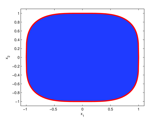
Figure 1: The convex set defined by $x_{1}^{2}+x_{2}^{2}\geq x_{1}^{4}+x_{1}^{2}x_{2}^{2}+x_{2}^{4}$.

The convex set $\{x\in\mathbb{R}^{2}:\,x_{1}^{2}+x_{2}^{2}\geq x_{1}^{4}+x_{1}^{2}x_{2}^{2}+x_{2}^{4}\}$ can be defined as $S_{\mathbb{R}^{2}}(f)$ with rational function $f(x)=1-\frac{x_{1}^{4}+x_{1}^{2}x_{2}^{2}+x_{2}^{4}}{x_{1}^{2}+x_{2}^{2}}$. The set $S_{\mathbb{R}^{2}}(f)$ is the shaded area bounded by a thick curve in Figure 1. We have already seen that $f(x)$ is first order sos concave. So $S_{\mathbb{R}^{2}}(f)=\mathcal{R}_{qmod}^{\mathbb{R}^{2}}(f)$. A polynomial division shows that $\frac{1}{x_{1}^{2}+x_{2}^{2}}\mathfrak{m}_{2}(x)\mathfrak{m}_{2}(x)^{T}$ equals

$$\begin{bmatrix}0&0&0&1&0&0\\ 0&1&0&x_{1}&x_{2}&0\\ 0&0&0&x_{2}&0&0\\ 1&x_{1}&x_{2}&x_{1}^{2}-x_{2}^{2}&x_{1}x_{2}&x_{2}^{2}\\ 0&x_{2}&0&x_{1}x_{2}&x_{2}^{2}&0\\ 0&0&0&x_{2}^{2}&0&0\end{bmatrix}+\frac{1}{p(x)}\begin{bmatrix}1&x_{1}&x_{2}&-x_{2}^{2}&x_{1}x_{2}&x_{2}^{2}\\ x_{1}&-x_{2}^{2}&x_{1}x_{2}&-x_{1}x_{2}^{2}&-x_{2}^{3}&x_{1}x_{2}^{2}\\ x_{2}&x_{1}x_{2}&x_{2}^{2}&-x_{2}^{3}&x_{1}x_{2}^{2}&x_{2}^{3}\\ -x_{2}^{2}&-x_{1}x_{2}^{2}&-x_{2}^{3}&x_{2}^{4}&-x_{1}x_{2}^{3}&-x_{2}^{4}\\ x_{1}x_{2}&-x_{2}^{3}&x_{1}x_{2}^{2}&-x_{1}x_{2}^{3}&-x_{2}^{4}&x_{1}x_{2}^{3}\\ x_{2}^{2}&x_{1}x_{2}^{2}&x_{2}^{3}&-x_{2}^{4}&x_{1}x_{2}^{3}&x_{2}^{4}\end{bmatrix}.$$

So we can see that $S_{\mathbb{R}^{2}}(f)=\mathcal{R}_{qmod}^{\mathbb{R}^{2}}(f)$ can be represented as

$$\left\{\begin{array}[]{l}(x_{1},x_{2})\in\mathbb{R}\times\mathbb{R}:\qquad\exists\quad y_{ij},z_{ij},\quad s.t.\qquad 1\geq y_{20}+z_{04},\\ \begin{bmatrix}0&0&0&1&0&0\\ 0&1&0&x_{1}&x_{2}&0\\ 0&0&0&x_{2}&0&0\\ 1&x_{1}&x_{2}&y_{20}-y_{02}&y_{11}&y_{02}\\ 0&x_{2}&0&y_{11}&y_{02}&0\\ 0&0&0&y_{02}&0&0\end{bmatrix}+\begin{bmatrix}z_{00}&z_{10}&z_{01}&-z_{02}&z_{11}&z_{02}\\ z_{10}&-z_{02}&z_{11}&-z_{12}&-z_{03}&z_{12}\\ z_{01}&z_{11}&z_{02}&-z_{03}&z_{12}&z_{03}\\ -z_{02}&-z_{12}&-z_{03}&z_{04}&-z_{13}&-z_{04}\\ z_{11}&-z_{03}&z_{12}&-z_{13}&-z_{04}&z_{13}\\ z_{02}&z_{12}&z_{03}&-z_{04}&z_{13}&z_{04}\end{bmatrix}\succeq 0\end{array}\right\}.$$

The plot of the projection of the above coincides with the shaded area in Figure 1.

3.3 Some special cases

3.3.1 Epigraph of rational functions

The rational function $f(x)$ is convex over the convex domain $\mathcal{D}$ if and only if its epigraph

$$\mathbf{epi}(f):=\{(x,t)\in\mathcal{D}\times\mathbb{R}:\,f(x)\leq t\}$$

is convex. The LMI $\mathcal{R}_{qmod}^{\mathcal{D}}(t-f)$ and $\mathcal{R}_{pre}^{\mathcal{D}}(t-f)$ can be constructed by thinking of $t-f(x)$ as a polynomial in $x$ with coefficients in $t$. So, if $f(x)$ is q-module (resp. preordering) convex over $\mathcal{D}$, $\mathcal{R}_{qmod}^{\mathcal{D}}(t-f)$ (resp. $\mathcal{R}_{pre}^{\mathcal{D}}(t-f)$) is an SDP representation for $\mathbf{epi}(f)$.

Now we consider the special case that $f(x)=\frac{q(x)}{p(x)}$ is a univariate rational function convex over an interval $I=[a,b]$ and $p(x)$ is positive over $(a,b)$. Note that $I=\{x\in\mathbb{R}:x-a\geq 0,b-x\geq 0\}$ ($x-a\geq 0$ is not required if $a=-\infty$, and similarly for $b-x\geq 0$).

Theorem 3.6.

Let $f(x)=\frac{q(x)}{p(x)}$ be a univariate rational function and $p(x)$ is a polynomial nonnegative over an interval $I$. If $f(x)$ is convex over $I$, then its epigraph $\mathbf{epi}(f)=\mathcal{R}_{qmod}^{I}(f)$.

Proof.

First assume $I=[a,b]$ is finite. Since $\mathcal{R}_{qmod}^{[a,b]}(f)$ is linear in $t$, it suffices to show for any fixed $t$

$$\{x\in[a,b]:\,\exists y,z,s.t.,\,x=y_{1},(y,z,t)\in\mathcal{R}_{qmod}^{[a,b]}(f)\}=\{x\in[a,b]:f(x)\leq t\}.$$

In the above the right hand side is contained in the left hand side. Now we prove the converse. For a contradiction, suppose there exists a tuple $(\hat{y},\hat{z},t)\in\mathcal{R}_{qmod}^{[a,b]}(f)$ such that and $\hat{x}=\hat{y}_{1}$ does not belong to the convex set $\{x\in[a,b]:f(x)\leq t\}$. Then there exists an affine function $c_{0}+c_{1}x$ such that

$$c_{0}+c_{1}\hat{x}<0,\quad c_{0}+c_{1}x\geq 0,\quad\forall\,x\in[a,b]:f(x)\leq t.$$

Since $f(x)$ is convex over [a,b], by optimality condition, there exists $\lambda\geq 0$ such that

$$c_{0}+c_{1}x-\lambda(t-f(x))=\frac{(c_{0}+c_{1}x-\lambda t)p(x)+\lambda q(x)}{p(x)}\geq 0,\quad\forall\,x\in[a,b].$$

Then we can see that $(c_{0}+c_{1}x-\lambda t)p(x)+\lambda q(x)$ is a univariate polynomial nonnegative on $[a,b]$. So there exist sos polynomials $s_{0}(x),s_{1}(x),s_{2}(x)$ of degrees at most $2d,2d-2,2d-2$ respectively (assume $\deg(p)+1,\deg(q)\leq 2d$ and see Powers and Reznick [15]) such that

$$(c_{0}+c_{1}x-\lambda t)p(x)+\lambda q(x)=s_{0}(x)+(x-a)s_{1}(x)+(b-a)s_{2}(x)$$

and hence then

$$c_{0}+c_{1}x=\lambda(t-f(x))+\frac{s_{0}(x)+(x-a)s_{1}(x)+(b-a)s_{2}(x)}{p(x)}.$$

Write $s_{0}(x),s_{1}(x),s_{2}(x)$ as

$$s_{0}(x)=\mathfrak{m}_{d}(x)^{T}W_{0}\mathfrak{m}_{d}(x),\quad s_{1}(x)=\mathfrak{m}_{d-1}(x)^{T}W_{1}\mathfrak{m}_{d-1}(x),\quad s_{2}(x)=\mathfrak{m}_{d-1}(x)^{T}W_{2}\mathfrak{m}_{d-1}(x)$$

for some symmetric $W_{0},W_{1},W_{2}\succeq 0$. Then we have (noting $g_{0}=1,g_{1}=x-a,g_{2}=b-x$ and (3.11))

$$a^{T}x-b =\lambda(t-f(x))+\sum_{i=0}^{2}\left(\frac{g_{i}(x)}{p(x)}\mathfrak{m}_{d-d_{i}}(x)\mathfrak{m}_{d-d_{i}}(x)^{T}\right)\bullet W_{i}\quad(d_{0}=0,d_{1}=d_{2}=1)$$

$$=\lambda(t-f(x))+\sum_{i=0}^{2}\left(\underset{\alpha\in\mathbb{N}:|\alpha|+|LE(p)|\leq 2d}{\sum}Q_{\alpha}^{(i)}x^{\alpha}+\underset{\beta\in\mathbb{N}:\beta<LE(p)}{\sum}P_{\alpha}^{(i)}\frac{x^{\beta}}{p(x)}\right)\bullet W_{i}.$$

In the above identity, if we replace each $x^{\alpha}$ by $\hat{y}_{\alpha}$ and $\frac{x^{\beta}}{p(x)}$ by $\hat{z}_{\beta}$, then get the contradiction

$$a^{T}\hat{x}-b=\lambda(t-(f^{(1)})^{T}\hat{y}-(f^{(2)})^{T}\hat{z})+\sum_{i=0}^{2}Q_{i}(\hat{y},\hat{z})\bullet W_{i}\geq 0.$$

Therefore we get $\mathbf{epi}(f)=\mathcal{R}_{qmod}^{[a,b]}(f)$.

When $I$ is an infinite interval of the form $[a,\infty)=\{x:x-a\geq 0\}$, $(-\infty,b]=\{x:b-x\geq 0\}$ or $(-\infty,\infty)=\{x:1\geq 0\}$, a similar argument can be applied to prove $\mathbf{epi}(f)=\mathcal{R}_{qmod}^{I}(f)$. ∎

3.3.2 Convex sets defined by structured rational functions

For the convenience of discussion, we define some basic convex sets ($r\leq s$)

$$K_{r,s}=\{(w,v)\in\mathbb{R}_{+}^{r}\times\mathbb{R}_{+}:\,w_{1}\cdots w_{r}\geq v^{s}\}$$ (3.16)

which are all SDP representable (see §3.3 in [1]).

First, consider epigraphs of rational functions of the form

$$f(x)=\frac{\sum_{i=1}^{P}(q_{i}(x))^{s_{i}}}{p_{1}(x)\cdots p_{r}(x)}$$ (3.17)

where $q_{i}(x),p_{j}(x)$ are polynomials nonnegative over $\mathcal{D}$ and the integer $s_{i}\geq r+1$. Then

$$\mathbf{epi}(f)=\left\{(x,t)\in\mathcal{D}\times\mathbb{R}:\,\sum_{i=1}^{P}(q_{i}(x))^{s_{i}}\leq p_{1}(x)\cdots p_{r}(x)t\right\}.$$

The epigraph $\mathbf{epi}(f)$ can be equivalently presented as

$$\mathbf{epi}(f)=\left\{(x,t)\in\mathcal{D}\times\mathbb{R}:\,\exists u_{i},w_{i},\,\sum_{i=1}^{P}\frac{u_{i}^{s_{i}}}{w_{1}\cdots w_{r}}\leq t,q_{i}(x)\leq u_{i},w_{i}\leq p_{i}(x),i=1,\ldots,P\right\}.$$

Note that

$$q_{i}(x)\leq u_{i}\Longleftrightarrow(x,u_{i})\in\mathbf{epi}(q_{i}),\qquad w_{i}\leq p_{i}(x)\Longleftrightarrow(x,-w_{i})\in\mathbf{epi}(-p_{i}),$$

$$\sum_{i=1}^{P}\frac{u_{i}^{s_{i}}}{w_{1}\cdots w_{r}}\leq t\Longleftrightarrow\exists v_{1},\cdots,v_{P}\geq 0,\,v_{1}+\cdots+v_{P}\leq t,(w_{1},\cdots,w_{r},v_{i},u_{i})\in K_{r+1,s_{i}}.$$

Hence we obtain that

$$\mathbf{epi}(f)=\Big{\{}(x,t)\in\mathcal{D}\times\mathbb{R}:\,\exists u_{i},w_{i},v_{i},\,\sum_{i=1}^{P}v_{i}\leq t,(w_{1},\cdots,w_{r},v_{i},u_{i})\in K_{r+1,s_{i}},$$

$$(x,u_{i})\in\mathbf{epi}(q_{i}),(x,-w_{i})\in\mathbf{epi}(-p_{i}),i=1,\ldots,P\Big{\}}.$$

When $q_{i}(x)$ are q-module (resp. preordering) convex over $\mathcal{D}$, we know $\mathbf{epi}(q_{i})=\mathcal{L}_{qmod}^{\mathcal{D}}(u_{i}-q_{i})$ (resp. $\mathbf{epi}(q_{i})=\mathcal{L}_{pre}^{\mathcal{D}}(u_{i}-q_{i})$), and similarly for $-p_{i}(x)$. Thus, we get the theorem:

Theorem 3.7.

Suppose $f(x)$ is given in the form (3.17) and all $q_{i}(x),p_{j}(x)$ there are nonnegative over $\mathcal{D}$.

(i)

If all $q_{i}(x),-p_{j}(x)$ are q-module convex over $\mathcal{D}$, then

$$\mathbf{epi}(f)=\Big{\{}(x,t):\,\exists u_{i},w_{i},v_{i},x\in\bigcap_{i=1}^{P}\mathcal{L}_{qmod}^{\mathcal{D}}(u_{i}-q_{i})\bigcap_{j=1}^{P}\mathcal{L}_{qmod}^{\mathcal{D}}(p_{j}-w_{j}),$$

$$\sum_{i=1}^{P}v_{i}\leq t,(w_{1},\cdots,w_{r},v_{i},u_{i})\in K_{r+1,s_{i}}\Big{\}}.$$

(ii)

If all $q_{i}(x),-p_{j}(x)$ are preordering convex over $\mathcal{D}$, then

$$\mathbf{epi}(f)=\Big{\{}(x,t):\,\exists u_{i},w_{i},v_{i},x\in\bigcap_{i=1}^{P}\mathcal{L}_{pre}^{\mathcal{D}}(u_{i}-q_{i})\bigcap_{j=1}^{P}\mathcal{L}_{pre}^{\mathcal{D}}(p_{j}-w_{j}),$$

$$\sum_{i=1}^{P}v_{i}\leq t,(w_{1},\cdots,w_{r},v_{i},u_{i})\in K_{r+1,s_{i}}\Big{\}}.$$

Example 3.8.

(i) Consider the epigraph $\left\{(x_{1},x_{2},t)\in\mathbb{R}_{+}\times\mathbb{R}\times\mathbb{R}:t\geq\frac{(1+x_{2}^{2})^{2}}{x_{1}}\right\}.$ The rational function here is given in the form (3.17). By Theorem 3.7, its epigraph can be represented as

$$\left\{(x_{1},x_{2},t):\,\exists\,u,\,\begin{bmatrix}t&u\\ u&x_{1}\end{bmatrix}\succeq 0,\,\begin{bmatrix}u-1&x_{2}\\ x_{2}&1\end{bmatrix}\succeq 0\right\}.$$

(ii) Consider the epigraph $\left\{(x,t)\in B(0,1)\times\mathbb{R}:\,t\geq\frac{(\sum_{i}x_{i}^{2})^{n+1}}{(1-x_{1}^{2})\cdots(1-x_{n}^{2})}\right\}.$ The rational function here is given in the form (3.17). By Theorem 3.7, its epigraph can be represented as

$$\left\{(x,t):\exists\,u,v_{i},w_{i},\,s.t.,\,\sum_{i=1}^{n}v_{i}\leq t,\begin{bmatrix}1-w_{i}&x_{i}\\ x_{i}&1\end{bmatrix}\succeq 0,\begin{bmatrix}u&x^{T}\\ x&I_{n}\end{bmatrix}\succeq 0,(u,w_{1},\ldots,w_{n},u)\in K_{n+1,n+1}\right\}.$$

Second, consider epigraphs of rational functions of the form

$$h(x)=\sum_{k=1}^{L}(f_{k}(x))^{b_{k}}$$ (3.18)

where $f_{k}(x)$ are rational functions given in form (3.17) and $b_{k}\geq 1$. Then the epigraph $\mathbf{epi}(h)=\{(x,t)\in\mathcal{D}\times\mathbb{R}:h(x)\leq t\}$ can be presented as

$$\mathbf{epi}(h)=\left\{(x,t):\,\exists\eta_{k},\tau_{k},\,\,\,\sum_{k=1}^{L}\tau_{k}\leq t,(x,\eta_{k})\in\mathbf{epi}(f_{k}),\,(\tau_{k},\eta_{k})\in K_{1,b_{k}},\,k=1,\cdots,L\right\}.$$

Once the SDP representation for each $\mathbf{epi}(f_{k})$ is available, one SDP representation for $\mathbf{epi}(h)$ can be obtained consequently from the above.

Example 3.9.

Consider the epigraph $\left\{(x_{1},x_{2},t)\in\mathbb{R}_{+}\times\mathbb{R}_{+}\times\mathbb{R}:\,t\geq\left(\frac{1+x_{2}^{2}}{x_{1}}\right)^{2}\right\}.$ From the above discussion, we know it can be represented as

$$\left\{(x_{1},x_{2},t):\,\exists\,u,\,\begin{bmatrix}t&u\\ u&1\end{bmatrix}\succeq 0,\,\begin{bmatrix}x_{1}&0&1\\ 0&x_{1}&x_{2}\\ 1&x_{2}&u\end{bmatrix}\succeq 0\right\}.$$

Third, consider the convex sets given in the form

$$T=\left\{x\in\mathcal{D}:a(x)\geq\sum_{k=1}^{J}h_{k}(x)\right\}$$ (3.19)

where $a(x)$ is a polynomial and every $h_{k}(x)$ is given in the form (3.18). Then

$$T=\left\{x:\,\exists t,\theta_{1},\cdots,\theta_{J},\,t\geq\sum_{k=1}^{J}\theta_{k},\,(x,-t)\in\mathbf{epi}(-a(x)),(x,\theta_{k})\in\mathbf{epi}(h_{k}(x)),k=1,\ldots,J\right\}.$$

When $a(x)$ is q-module or preordering concave over $\mathcal{D}$, $\mathbf{epi}(-a(x))$ is representable by $\mathcal{L}_{qmod}^{\mathcal{D}}(a(x)-t)$ or $\mathcal{L}_{pre}^{\mathcal{D}}(a(x)-t)$. Once the SDP representations for $\mathbf{epi}(-a(x))$ and all $\mathbf{epi}(h_{k}(x))$ are available, an SDP representation for $T$ can be obtained consequently.

Example 3.10.

(i) Consider the convex set $T=\left\{(x_{1},x_{2})\in\mathbb{R}_{+}\times\mathbb{R}:\,1-3x_{2}^{2}\geq\frac{(1+x_{2}^{2})^{2}}{x_{1}}\right\}.$ It is given in the form (3.19) with $\mathcal{D}=\mathbb{R}_{+}\times\mathbb{R}$. From the above discussion, we have

$$T=\left\{(x_{1},x_{2}):\,\exists\,u,w,\,\begin{bmatrix}1-u&x_{2}\\ x_{2}&\frac{1}{3}\end{bmatrix}\succeq 0,\,\begin{bmatrix}w-1&x_{2}\\ x_{2}&1\end{bmatrix}\succeq 0,\,(u,x_{1},w)\in K_{2,2}\right\}.$$

Note that $(u,x_{1},w)\in K_{2,2}$ has the representation $\begin{bmatrix}u&w\\ w&x_{1}\end{bmatrix}\succeq 0.$
(ii) Consider the convex set $T=\left\{(x_{1},x_{2})\in\mathbb{R}_{+}\times\mathbb{R}:\,1-x_{2}^{2}\geq\frac{(1+x_{2}^{2})^{2}}{x_{1}^{2}}\right\}.$ It is given in the form (3.19) with $\mathcal{D}=\mathbb{R}_{+}\times\mathbb{R}$. From the above discussion, we know it can be represented as

$$\left\{(x_{1},x_{2}):\,\exists\,u,\,\begin{bmatrix}1+u&x_{2}\\ x_{2}&1-u\end{bmatrix}\succeq 0,\,\begin{bmatrix}x_{1}&0&1\\ 0&x_{1}&x_{2}\\ 1&x_{2}&u\end{bmatrix}\succeq 0\right\}.$$

4 Convex sets with singularities

Let $S_{\mathcal{D}}(f)=\{x\in\mathcal{D}:f(x)\geq 0\}$ be a convex set defined by a polynomial or rational function $f(x)$. Here $\mathcal{D}=\{x\in\mathbb{R}^{n}:\,g_{1}(x)\geq 0,\cdots,g_{m}(x)\geq 0\}$ is still a convex domain defined by polynomials. Suppose the origin belongs to $S_{\mathcal{D}}(f)$ and is a singular point of the hypersurface $\mathcal{Z}(f)=\{x\in\mathbb{C}^{n}:\,f(x)=0\}$, i.e.,

$$f(0,0)=0,\,\nabla f(0,0)=0.$$

We are interested in finding SDP representability conditions for $S_{\mathcal{D}}(f)$.

As we have seen in Introduction, one natural approach to getting an SDP representation for $S_{\mathcal{D}}(f)$ is to find a “nicer” defining function (possibly a concave rational function). Let $p(x)$ be a polynomial or rational function positive in $int(\mathcal{D})$. Then we can see $S_{\mathcal{D}}(f)$ is the closure of the set

$$\left\{x\in int(\mathcal{D}):\frac{f(x)}{p(x)}\geq 0\right\}.$$

If $\frac{f(x)}{p(x)}$ has nice properties, e.g., $\frac{f(x)}{p(x)}$ has special structures discussed in Section 3, or it is q-module or preordering concave over $\mathcal{D}$, then an explicit SDP representation for $S_{\mathcal{D}}(f)$ can be obtained. For instance, consider the convex set

$$\{(x_{1},x_{2})\in\mathbb{R}_{+}^{2}:\,-x_{1}^{3}+3x_{1}x_{2}^{2}-(x_{1}^{2}+x_{2}^{2})^{2}\geq 0\}.$$

The origin is a singular point on its boundary. If we choose $p(x)=x_{2}^{2}$, then it can be presented as

$$\left\{(x_{1},x_{2})\in\mathbb{R}_{+}^{2}:\,3x_{1}\geq 2x_{1}^{2}+x_{2}^{2}+\frac{x_{1}^{3}}{x_{2}^{2}}+\frac{x_{1}^{4}}{x_{2}^{2}}\right\}.$$

Then this set can be represented as

$$\Big{\{}(x_{1},x_{2})\in\mathbb{R}_{+}^{2}:\,\exists\,u_{1},u_{2},u_{3},u_{4},\,\,s.t.,\,3x_{1}\geq 2u_{1}+u_{2}+u_{3}+u_{4},\,(u_{1},x_{1})\in K_{1,2},$$

$$\qquad(u_{2},x_{2})\in K_{1,2},(u_{3},x_{2},x_{2},x_{1})\in K_{3,3},(u_{4},x_{2},x_{2},x_{1})\in K_{3,4}\Big{\}}.$$

However, there is no general procedure to find such a nice function $p(x)$. In convex analysis, there is a technique called perspective transformation which might be very useful now. Generally, we can assume

$$S_{\mathcal{D}}(f)\subset\mathbb{R}_{+}\times\mathbb{R}^{n-1},\qquad int(S_{\mathcal{D}}(f))\neq\emptyset.$$

Define the perspective transformation $\mathfrak{p}$ as

$$\mathfrak{p}(x_{1},x_{2},\cdots,x_{n})=(1/x_{1},x_{2}/x_{1},\cdots,x_{n}/x_{1}).$$

The image of $S_{\mathcal{D}}(f)$ under the perspective transformation $\mathfrak{p}$ is

$$\Big{\{}\left(1/x_{1},x_{2}/x_{1},\cdots,x_{n}/x_{1}\right):\,x\in S_{\mathcal{D}}(f)\Big{\}}\subset\mathbb{R}_{+}\times\mathbb{R}^{n-1},$$

which is also convex (see §2.3 in [2]). Define new coordinates

$$\tilde{x}_{1}=\frac{1}{x_{1}},\quad\tilde{x}_{2}=\frac{x_{2}}{x_{1}},\quad\cdots,\quad\tilde{x}_{n}=\frac{x_{n}}{x_{1}}.$$

Denote $\tilde{\tilde{x}}=(\tilde{x}_{2},\cdots,\tilde{x}_{n})$. Suppose $f(x)$ has Laurent expansion around the origin

$$f(x)=f_{b}(x)-f_{b+1}(x)-\cdots-f_{d}(x)$$

where every $f_{k}(x)$ is a homogeneous part of degree $k$. Let

$$\tilde{f}(\tilde{x}):=\tilde{f}_{0}(\tilde{\tilde{x}})-\frac{\tilde{f}_{1}(\tilde{\tilde{x}})}{\tilde{x}_{1}}-\cdots-\frac{\tilde{f}_{d-b}(\tilde{\tilde{x}})}{\tilde{x}_{1}^{d-b}}$$

where $\tilde{f}_{i}(\tilde{x}_{2},\cdots,\tilde{x}_{n}):=x_{1}^{b+i}f_{b+i}(\tilde{x})$. Define a new domain $\tilde{\mathcal{D}}$ as

$$\tilde{\mathcal{D}}=\{\tilde{x}\in\mathbb{R}^{n}:\,\tilde{g}_{1}(\tilde{x})\geq 0,\cdots,\tilde{g}_{m}(\tilde{x})\geq 0\}$$

where $\tilde{g}_{i}(\tilde{x})=\frac{g_{i}(x)}{x_{1}^{\deg(g_{i})}}$. Note that $\tilde{\mathcal{D}}$ is convex if and only if $\mathcal{D}$ is convex (see §2.3 in [2]). Therefore, under the perspective transformation $\mathfrak{p}$, the set $S_{\mathcal{D}}(f)$ can be equivalently defined as

$$S_{\tilde{\mathcal{D}}}(\tilde{f})=\{\tilde{x}\in\tilde{\mathcal{D}}:\tilde{f}(\tilde{x})\geq 0\}.$$

Proposition 4.1.

If $S_{\mathcal{D}}(f)$ is convex, then $\tilde{f}_{0}(\tilde{\tilde{x}})\geq 0$ for any $\tilde{x}=(\tilde{x}_{1},\tilde{\tilde{x}})\in S_{\tilde{\mathcal{D}}}(\tilde{f})$.

Proof.

Fix $x=(x_{1},\cdots,x_{n})\in S_{\mathcal{D}}(f)$ and $\tilde{x}=(\tilde{x}_{1},\cdots,\tilde{x}_{n})\in S_{\tilde{\mathcal{D}}}(\tilde{f})$ such that $\tilde{x}=\mathfrak{p}(x_{1},x_{2},\cdots,x_{n})$. By the convexity of $S_{\mathcal{D}}(f)$, the line segment $\{tx:0\leq t\leq 1\}$ belongs to $S_{\mathcal{D}}(f)$. Thus its image

$$\mathfrak{p}(tx_{1},tx_{2},\cdots,tx_{n})=(\frac{1}{t}\tilde{x}_{1},\tilde{x}_{2},\cdots,\tilde{x}_{n})$$

belongs to $S_{\tilde{\mathcal{D}}}(\tilde{f})$. Now let $t\to 0$. Then $\tilde{f}(\frac{1}{t}\tilde{x}_{1},\tilde{x}_{2},\cdots,\tilde{x}_{n})\geq 0$ implies $\tilde{f}_{0}(\tilde{\tilde{x}})\geq 0$. ∎

4.1 The case of structured $\tilde{f}_{k}(\tilde{\tilde{x}})$

In this subsection, we assume $\tilde{f}_{k}(\tilde{\tilde{x}})$ have special structures. Then the methods in Subsection 3.3.2 can be applied to construct SDP representations for $S_{\tilde{\mathcal{D}}}(\tilde{f})$.

Theorem 4.2.

Suppose every $\tilde{f}_{k}(\tilde{\tilde{x}})\,(k=1,\cdots,d-b)$ is given in the form

$$\tilde{f}_{k}(\tilde{\tilde{x}})=\sum_{i=1}^{L_{k}}(q_{k,i}(\tilde{\tilde{x}}))^{r_{k,i}}+\sum_{j=1}^{R_{k}}\Big{(}\sum_{\ell=1}^{Q_{k,j}}(p_{k,j,\ell}(\tilde{\tilde{x}}))^{s_{k,j,\ell}}\Big{)}^{k}$$

for some polynomials $q_{k,i}(\tilde{\tilde{x}}),p_{k,j,\ell}(\tilde{\tilde{x}})$ which are nonnegative over $\tilde{\mathcal{D}}$ and integers $r_{k,i}\geq k+1$, $s_{k,j,\ell}\geq 2$ ($p_{k,j}(\tilde{\tilde{x}})$ can be any affine polynomial when $s_{k,j,\ell}$ is even). Then $S_{\tilde{\mathcal{D}}}(\tilde{f})$ can be represented as

$$\left\{\tilde{x}:\,\exists\,u,u_{k,i},v_{k,j,\ell},\,u\geq\sum_{k=1}^{d-b}\left(\sum_{i=1}^{L_{k}}\frac{(u_{k,i})^{r_{k,i}}}{\tilde{x}_{1}^{k}}+\sum_{j=1}^{R_{k}}\left(\sum_{\ell=1}^{Q_{k,j}}\frac{(v_{k,j,\ell})^{s_{k,j,\ell}}}{\tilde{x}_{1}}\right)^{k}\right)\right.,$$

$$(\tilde{\tilde{x}},-u)\in\mathbf{epi}(-\tilde{f}_{0}),\,(\tilde{\tilde{x}},u_{k,i})\in\mathbf{epi}(q_{k,i}),\,(\tilde{\tilde{x}},v_{k,j,\ell})\in\mathbf{epi}(p_{k,j,\ell})\Big{\}}.$$

Furthermore, if $-\tilde{f}_{0}(\tilde{\tilde{x}})$ and all $q_{k,j}(\tilde{\tilde{x}}),p_{k,j,\ell}(\tilde{\tilde{x}})$ are q-module or preordering convex over $\tilde{\mathcal{D}}$, then $S_{\tilde{\mathcal{D}}}(\tilde{f})$ is SDP representable.

Proof.

The first conclusion is obvious by introducing new variables $u,u_{k,i},v_{k,j,\ell}$. Note that

$$u\geq\sum_{k=1}^{d-b}\Big{(}\sum_{i=1}^{L_{k}}\frac{(u_{k,i})^{r_{k,i}}}{\tilde{x}_{1}^{k}}+\sum_{j=1}^{R_{k}}\Big{(}\sum_{\ell=1}^{Q_{k,j}}\frac{(v_{k,j,\ell})^{s_{k,j,\ell}}}{\tilde{x}_{1}}\Big{)}^{k}\Big{)}$$

is equivalent to

$$u\geq\sum_{k=1}^{d-b}\Big{(}\sum_{i=1}^{L_{k}}\eta_{k,i}+\sum_{j=1}^{R_{k}}\xi_{k}\Big{)},(\tilde{x}_{1},\cdots,\tilde{x}_{1},\,\,\eta_{k,i},u_{k,i}) \in K_{k+1,r_{k,i}},$$

$$(\xi_{k},\zeta_{k})\in K_{1,k},\,\,(\zeta_{k},\tilde{x}_{1},v_{k,j,\ell}) \in K_{2,s_{k,j,\ell}}.$$

When $-\tilde{f}_{0}(\tilde{\tilde{x}})$ is q-module (resp. preordering) convex over $\tilde{\mathcal{D}}$, $(\tilde{\tilde{x}},-u)\in\mathbf{epi}(-\tilde{f}_{0})$ is representable by $\mathcal{L}_{qmod}^{\tilde{\mathcal{D}}}(u-\tilde{f}_{0})$ (resp. $\mathcal{L}_{pre}^{\tilde{\mathcal{D}}}(u-\tilde{f}_{0})$). Similar results hold for $q_{k,j}(\tilde{\tilde{x}}),p_{k,j,\ell}(\tilde{\tilde{x}})$. Once the SDP representations for epigraphs of $-\tilde{f}_{0}(\tilde{\tilde{x}})$, $q_{k,j}(\tilde{\tilde{x}})$ and $p_{k,j,\ell}(\tilde{\tilde{x}})$ are all available, we can get an SDP representation for $S_{\tilde{\mathcal{D}}}(\tilde{f})$ consequently. ∎

Now we show some examples on how to apply Theorem 4.2.

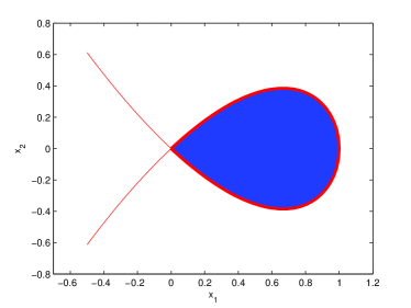
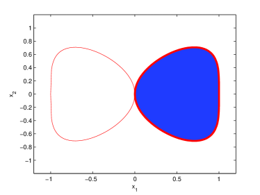
(a): $x_{1}^{2}-x_{1}^{3}-x_{2}^{2}\geq 0,x_{1}\geq 0$	(b): $x_{1}^{2}-x_{1}^{4}-x_{2}^{4}\geq 0,x_{1}\geq 0$
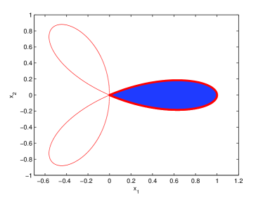
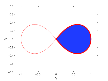
(c): $x_{1}^{3}-3x_{1}x_{2}^{2}-(x_{1}^{2}+x_{2}^{2})^{2}\geq 0,x_{1}\geq 0$	(d): $x_{1}^{2}-x_{2}^{2}-(x_{1}^{2}+x_{2}^{2})^{2}\geq 0,x_{1}\geq 0$

Figure 2: Four singular convex sets discussed in Example 4.3

.

Example 4.3.

(a) Consider convex set $S=\{(x_{1},x_{2})\in\mathbb{R}_{+}\times\mathbb{R}:\,x_{1}^{2}-x_{1}^{3}-x_{2}^{2}\geq 0\}.$ Its boundary is a cubic curve and the origin is a singular node. This convex set is the shaded area bounded by a thick curve in Figure 2(a). The thin curves are other branches of this cubic curve. After the perspective transformation, we get

$$\tilde{S}=\left\{(\tilde{x}_{1},\tilde{x}_{2})\in\mathbb{R}_{+}\times\mathbb{R}:\,1-\tilde{x}_{2}^{2}-\frac{1}{\tilde{x}_{1}}\geq 0\right\}$$

which can be represented as

$$\left\{(\tilde{x}_{1},\tilde{x}_{2}):\,\exists\,u,\,\,s.t.,\,\begin{bmatrix}1-u&\tilde{x}_{2}\\ \tilde{x}_{2}&1\end{bmatrix}\succeq 0,\,\begin{bmatrix}u&1\\ 1&\tilde{x}_{1}\end{bmatrix}\succeq 0\right\}.$$

After the inverse perspective transformation, we get

$$S=\left\{(x_{1},x_{2}):\,\exists\,u,\,\,s.t.,\,\begin{bmatrix}x_{1}-u&x_{2}\\ x_{2}&x_{1}1\end{bmatrix}\succeq 0,\,\begin{bmatrix}u&x_{1}\\ x_{1}&x_{1}\end{bmatrix}\succeq 0\right\}.$$

The plot of the projection of the above coincides with the shaded area in Figure 2(a).
(b) Consider convex set $S=\{(x_{1},x_{2})\in\mathbb{R}_{+}\times\mathbb{R}:\,x_{1}^{2}-x_{2}^{4}-x_{2}^{4}\geq 0\}.$ The origin is a singular tacnode on the boundary. This convex set is the shaded area bounded by a thick curve in Figure 2(b). The thin curve is the other branch of the singular curve $x_{1}^{2}-x_{2}^{4}-x_{2}^{4}=0$. After the perspective transformation, we get

$$\tilde{S}=\left\{(\tilde{x}_{1},\tilde{x}_{2})\in\mathbb{R}_{+}\times\mathbb{R}:\,1\geq\frac{1+\tilde{x}_{2}^{4}}{\tilde{x}_{1}^{2}}\right\}$$

which can be represented as

$$\left\{(\tilde{x}_{1},\tilde{x}_{2}):\,\exists\,u_{1},u_{2},\,\,s.t.,\,\begin{bmatrix}1-u_{1}&u_{2}\\ u_{2}&1+u_{1}\end{bmatrix}\succeq 0,\,\begin{bmatrix}u_{1}&1\\ 1&\tilde{x}_{1}\end{bmatrix}\succeq 0,\,\begin{bmatrix}u_{2}&\tilde{x}_{2}\\ \tilde{x}_{2}&\tilde{x}_{1}\end{bmatrix}\succeq 0\right\}.$$

After the inverse perspective transformation, we get

$$S=\left\{(x_{1},x_{2}):\,\exists\,u_{1},u_{2},\,\,s.t.,\,\begin{bmatrix}x_{1}-u_{1}&u_{2}\\ u_{2}&x_{1}+u_{1}\end{bmatrix}\succeq 0,\,\begin{bmatrix}u_{1}&x_{1}\\ x_{1}&1\end{bmatrix}\succeq 0,\,\begin{bmatrix}u_{2}&x_{2}\\ x_{2}&1\end{bmatrix}\succeq 0\right\}.$$

The plot of the projection of the above coincides with the shaded area in Figure 2(b).
(c) Consider convex set $S=\{(x_{1},x_{2})\in\mathbb{R}_{+}\times\mathbb{R}:\,x_{1}^{3}-3x_{1}x_{2}^{2}-(x_{1}^{2}+x_{2}^{2})^{2}\geq 0\}.$ The origin is a singular point on the boundary. This convex set is the shaded area bounded by a thick curve in Figure 2(c). The thin curves are other branches of the singular curve $x_{1}^{3}-3x_{1}x_{2}^{2}-(x_{1}^{2}+x_{2}^{2})^{2}=0$. After the perspective transformation, we get

$$\tilde{S}=\left\{(\tilde{x}_{1},\tilde{x}_{2})\in\mathbb{R}_{+}\times\mathbb{R}:\,1-3\tilde{x}_{2}^{2}-\frac{(1+\tilde{x}_{2}^{2})^{2}}{\tilde{x}_{1}}\geq 0\right\}$$

which can be represented as

$$\left\{(\tilde{x}_{1},\tilde{x}_{2}):\,\exists\,u,w,\,\,s.t.,\,\begin{bmatrix}1-u&\tilde{x}_{2}\\ \tilde{x}_{2}&\frac{1}{3}\end{bmatrix}\succeq 0,\,\begin{bmatrix}u&w\\ w&\tilde{x}_{1}\end{bmatrix}\succeq 0,\,\begin{bmatrix}w-1&\tilde{x}_{2}\\ \tilde{x}_{2}&1\end{bmatrix}\succeq 0\right\}.$$

After the inverse perspective transformation, we get

$$S=\left\{(x_{1},x_{2}):\,\exists\,u,w,\,s.t.,\,\begin{bmatrix}x_{1}-u&x_{2}\\ x_{2}&\frac{1}{3}x_{1}\end{bmatrix}\succeq 0,\,\begin{bmatrix}u&w\\ w&1\end{bmatrix}\succeq 0,\,\begin{bmatrix}w-x_{1}&x_{2}\\ x_{2}&x_{1}\end{bmatrix}\succeq 0\right\}.$$

The plot of the projection of the above coincides with the shaded area in Figure 2(c).
(d) Consider convex set $S=\{(x_{1},x_{2})\in\mathbb{R}_{+}\times\mathbb{R}:\,x_{1}^{2}-x_{2}^{2}-(x_{1}^{2}+x_{2}^{2})^{2}\geq 0\}.$ The origin is a singular point on the boundary which is one branch of the lemniscate curve $x_{1}^{2}-x_{2}^{2}-(x_{1}^{2}+x_{2}^{2})^{2}=0$. This convex set is the shaded area bounded a thick lemniscate curve in Figure 2(d). The thin curve is the other branch of the lemniscate curve. After the perspective transformation, we get

$$\tilde{S}=\left\{(\tilde{x}_{1},\tilde{x}_{2})\in\mathbb{R}_{+}\times\mathbb{R}:\,(1-\tilde{x}_{2}^{2})\geq\left(\frac{1+\tilde{x}_{2}^{2}}{\tilde{x}_{1}}\right)^{2}\right\}$$

which can be represented as

$$\left\{(\tilde{x}_{1},\tilde{x}_{2}):\,\exists\,u,w,\,\,s.t.\,\begin{bmatrix}1+u&\tilde{x}_{2}\\ \tilde{x}_{2}&1-u\end{bmatrix}\succeq 0,\,\begin{bmatrix}u&1&\tilde{x}_{2}\\ 1&\tilde{x}_{1}&0\\ \tilde{x}_{2}&0&\tilde{x}_{1}\end{bmatrix}\succeq 0\right\}.$$

After the inverse perspective transformation, we get

$$S=\left\{(x_{1},x_{2}):\,\exists\,u,\,\,s.t.\,\begin{bmatrix}x_{1}+u&x_{2}\\ x_{2}&x_{1}-u\end{bmatrix}\succeq 0,\,\begin{bmatrix}u&x_{1}&x_{2}\\ x_{1}&1&0\\ x_{2}&0&1\end{bmatrix}\succeq 0\right\}.$$

The plot of the projection of the above coincides with the shaded area in Figure 2(d).

4.2 The case of two consecutive homogeneous parts

In this subsection, we consider the special case that $f(x)=f_{b}(x)-f_{b+1}(x)$ having two consecutive homogeneous parts. Then, after perspective transformation, we get

$$S_{\tilde{\mathcal{D}}}(\tilde{f})=\left\{\tilde{x}\in\tilde{\mathcal{D}}:\tilde{f}_{0}(\tilde{\tilde{x}})-\frac{\tilde{f}_{1}(\tilde{\tilde{x}})}{\tilde{x}_{1}}\geq 0\right\}.$$

By Proposition 4.1, for any $\tilde{x}\in\tilde{\mathcal{D}}$, we have $f_{0}(\tilde{\tilde{x}})\geq 0$. Let $\mathcal{D}^{\prime}$ be the intersection of $\{\tilde{\tilde{x}}:f_{0}(\tilde{\tilde{x}})\geq 0\}$ and the projection of $\mathcal{D}\subset\mathbb{R}_{+}\times\mathbb{R}^{n-1}$ into $\mathbb{R}^{n-1}$. Then we get

$$S_{\tilde{\mathcal{D}}}(\tilde{f})=\left\{(\tilde{\tilde{x}},\tilde{x}_{1})\in\mathcal{D}^{\prime}\times\mathbb{R}_{+}:\tilde{x}_{1}\geq h(\tilde{\tilde{x}})\right\},\quad h(\tilde{\tilde{x}}):=\frac{\tilde{f}_{1}(\tilde{\tilde{x}})}{\tilde{f}_{0}(\tilde{\tilde{x}})}.$$

Then $S_{\tilde{\mathcal{D}}}(\tilde{f})$ is the epigraph $\mathbf{epi}(h)$ of the rational function $h(\tilde{\tilde{x}})$ over $\mathcal{D}^{\prime}$. Note that $h(\tilde{\tilde{x}})$ is convex over the domain $\mathcal{D}^{\prime}$ if and only if $S_{\tilde{\mathcal{D}}}(\tilde{f})$ is convex, which then holds if and only if $S_{\mathcal{D}}(f)$ is convex. So, if $h(\tilde{\tilde{x}})$ is q-module or preordering convex over $\mathcal{D}^{\prime}$, then $\mathcal{R}_{qmod}^{\mathcal{D}^{\prime}}(\tilde{x}_{1}-h)$ or $\mathcal{R}_{pre}^{\mathcal{D}^{\prime}}(\tilde{x}_{1}-h)$ is an SDP representation for $\mathbf{epi}(h)$, and then one can be obtained for $S_{\mathcal{D}}(h)$ after the inverse perspective transformation.

A very interesting case is $n=2$. Then $\mathcal{D}^{\prime}$ must be an interval $I$ of the real line.

Theorem 4.4.

Let $n=2$ and $\mathcal{D}^{\prime}=I$ be an interval as above. If $S_{\mathcal{D}}(f)$ is convex, then $S_{\tilde{\mathcal{D}}}(\tilde{f})=\mathcal{R}_{qmod}^{I}(\tilde{x}_{1}-h)$, and hence $S_{\mathcal{D}}(f)=\mathfrak{p}^{-1}(\mathcal{R}_{qmod}^{I}(\tilde{x}_{1}-h))$.

Proof.

When $n=2$, $f(\tilde{\tilde{x}})$ is a univariate rational function. When $S_{\mathcal{D}}(f)$ is convex, $S_{\tilde{\mathcal{D}}}(\tilde{f})$ is also convex. Since $S_{\tilde{\mathcal{D}}}(\tilde{f})$ is the epigraph of $f(\tilde{\tilde{x}})$, $f(\tilde{\tilde{x}})$ must be a univariate rational function convex over the interval $I$. By Theorem 3.6, its epigraph is representable by $\mathcal{R}_{qmod}^{I}(\tilde{x}_{1}-h)$. Thus $S_{\tilde{\mathcal{D}}}(\tilde{f})=\mathcal{R}_{qmod}^{I}(\tilde{x}_{1}-h)$. After the inverse perspective transformation, we can get an SDP representation for $S_{\mathcal{D}}(f)$. ∎

Now we see some examples on how to find SDP representations for singular convex sets by applying Theorem 4.4.

Example 4.5.

(i) We revisit the singular convex set (a) in Example 4.3. After the perspective transformation, we get $\tilde{S}=\left\{(\tilde{x}_{1},\tilde{x}_{2})\in\mathbb{R}\times[-1,1]:\,\tilde{x}_{1}\geq\frac{1}{1-\tilde{x}_{2}^{2}}\right\},$ which can be represented as

$$\left\{(\tilde{x}_{1},\tilde{x}_{2}):\begin{array}[]{lr}\exists\,y_{2},y_{3},y_{4},z_{0},z_{1},&\tilde{x}_{1}\geq z_{0},\qquad\begin{bmatrix}1-y_{2}&\tilde{x}_{2}-y_{3}\\ \tilde{x}_{2}-y_{3}&y_{2}-y_{4}\end{bmatrix}\succeq 0,\\ \begin{bmatrix}1&\tilde{x}_{2}&y_{2}\\ \tilde{x}_{2}&y_{2}&y_{3}\\ y_{2}&y_{3}&y_{4}\end{bmatrix}\succeq 0,&\begin{bmatrix}z_{0}&z_{1}&-1+z_{0}\\ z_{1}&-1+z_{0}&-\tilde{x}_{2}+z_{1}\\ -1+z_{0}&-\tilde{x}_{2}+z_{1}&-y_{2}-1+z_{0}\end{bmatrix}\succeq 0\end{array}\right\}.$$

Applying the inverse perspective transformation, we get an SDP representation for $S$

$$\left\{(x_{1},x_{2}):\begin{array}[]{lr}\exists\,y_{2},y_{3},y_{4},z_{0},z_{1},&1\geq z_{0},\qquad\begin{bmatrix}x_{1}-y_{2}&x_{2}-y_{3}\\ x_{2}-y_{3}&y_{2}-y_{4}\end{bmatrix}\succeq 0,\\ \begin{bmatrix}x_{1}&x_{2}&y_{2}\\ x_{2}&y_{2}&y_{3}\\ y_{2}&y_{3}&y_{4}\end{bmatrix}\succeq 0,&\begin{bmatrix}z_{0}&z_{1}&-x_{1}+z_{0}\\ z_{1}&-x_{1}+z_{0}&-x_{2}+z_{1}\\ -x_{1}+z_{0}&-x_{2}+z_{1}&-y_{2}-x_{1}+z_{0}\end{bmatrix}\succeq 0\end{array}\right\}.$$

Interestingly but not surprisingly, the plot of the above coincides with the shaded area in Figure 2(a).
(ii) Revisit the singular convex set (c) in Example 4.3. After the perspective transformation, we get $\tilde{S}=\left\{(\tilde{x}_{1},\tilde{x}_{2})\in\mathbb{R}\times\frac{1}{\sqrt{3}}[-1,1]:\,\tilde{x}_{1}\geq-\frac{x_{2}^{2}}{3}-\frac{7}{9}+\frac{16}{9(1-3x_{2}^{2})}\right\},$ which equals

$$\left\{(\tilde{x}_{1},\tilde{x}_{2}):\begin{array}[]{lr}\exists\,y_{2},y_{3},y_{4},z_{0},z_{1},&\tilde{x}_{1}\geq-\frac{1}{3}y_{2}-\frac{7}{9}+\frac{16}{9}z_{0},\begin{bmatrix}1-3y_{2}&\tilde{x}_{2}-3y_{3}\\ \tilde{x}_{2}-3y_{3}&y_{2}-3y_{4}\end{bmatrix}\succeq 0,\\ \begin{bmatrix}1&\tilde{x}_{2}&y_{2}\\ \tilde{x}_{2}&y_{2}&y_{3}\\ y_{2}&y_{3}&y_{4}\end{bmatrix}\succeq 0,&\begin{bmatrix}z_{0}&z_{1}&\frac{1}{3}(z_{0}-1)\\ z_{1}&\frac{1}{3}(z_{0}-1)&\frac{1}{3}(z_{1}-\tilde{x}_{2})\\ \frac{1}{3}(z_{0}-1)&\frac{1}{3}(z_{1}-\tilde{x}_{2})&-\frac{1}{3}y_{2}+\frac{1}{9}(z_{0}-1)\end{bmatrix}\succeq 0\end{array}\right\}.$$

Applying the inverse perspective transformation, we get an SDP representation for $S$

$$\left\{(x_{1},x_{2}):\begin{array}[]{lr}\exists\,y_{2},y_{3},y_{4},z_{0},z_{1},&1\geq-\frac{1}{3}y_{2}-\frac{7}{9}x_{1}+\frac{16}{9}z_{0},\begin{bmatrix}x_{1}-3y_{2}&x_{2}-3y_{3}\\ x_{2}-3y_{3}&y_{2}-3y_{4}\end{bmatrix}\succeq 0,\\ \begin{bmatrix}x_{1}&x_{2}&y_{2}\\ x_{2}&y_{2}&y_{3}\\ y_{2}&y_{3}&y_{4}\end{bmatrix}\succeq 0,&\begin{bmatrix}z_{0}&z_{1}&\frac{1}{3}(z_{0}-x_{1})\\ z_{1}&\frac{1}{3}(z_{0}-x_{1})&\frac{1}{3}(z_{1}-x_{2})\\ \frac{1}{3}(z_{0}-x_{1})&\frac{1}{3}(z_{1}-x_{2})&-\frac{1}{3}y_{2}+\frac{1}{9}(z_{0}-x_{1})\end{bmatrix}\succeq 0\end{array}\right\}.$$

Also interestingly but not surprisingly, the plot of the above also coincides with the shaded area in Figure 2(c).

Now let us conclude this subsection with an example such that Theorem 4.4 can be applied to get an SDP representation for $S_{\mathcal{D}}(f)$ while Theorem 4.2 can not.

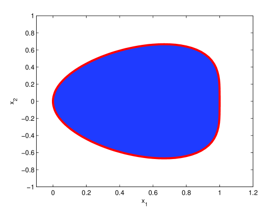
Figure 3: The singular convex set defined by $x_{1}(x_{1}^{2}+x_{2}^{2})-x_{1}^{4}-x_{1}^{2}x_{2}^{2}-x_{2}^{4}\geq 0$ .

Example 4.6.

Consider the convex set $S=\{(x_{1},x_{2})\in\mathbb{R}^{2}:\,x_{1}(x_{1}^{2}+x_{2}^{2})-x_{1}^{4}-x_{1}^{2}x_{2}^{2}-x_{2}^{4}\geq 0\}.$ The origin is a singular point on the boundary $\partial S$ which is a quartic bean curve. The picture of this convex set is the shaded area bounded by the thick bean curve in Figure 3. After the perspective transformation, we get $\tilde{S}=\left\{(\tilde{x}_{1},\tilde{x}_{2})\in\mathbb{R}^{2}:\,\tilde{x}_{1}\geq f(\tilde{x}_{2}):=\tilde{x}_{2}^{2}+\frac{1}{1+\tilde{x}_{2}^{2}}\right\}.$ $f(\tilde{x}_{2})$ does not have structures required by Theorem 4.2. Obviously $\mathcal{D}^{\prime}=(-\infty,\infty)$. We can check that $f(\tilde{x}_{2})$ is convex over $(-\infty,\infty)$, so its epigraph $\mathbf{epi}(f)=\mathcal{R}_{qmod}^{(-\infty,\infty)}(\tilde{x}_{1}-f)$ which can be represented as

$$\left\{(\tilde{x}_{1},\tilde{x}_{2}):\,\exists\,y_{2},z_{0},z_{1},\tilde{x}_{1}\geq y_{2}+z_{0},\begin{bmatrix}z_{0}&z_{1}&1-z_{0}\\ z_{1}&1-z_{0}&\tilde{x}_{2}-z_{1}\\ 1-z_{0}&\tilde{x}_{2}-z_{1}&y_{2}-1+z_{0}\end{bmatrix}\succeq 0\right\}.$$

A direct SDP representation of $S$ can be obtained by applying the inverse perspective transformation

$$\left\{(x_{1},x_{2}):\,\exists\,y_{2},z_{0},z_{1},\,1\geq y_{2}+z_{0},\begin{bmatrix}z_{0}&z_{1}&x_{1}-z_{0}\\ z_{1}&x_{1}-z_{0}&x_{2}-z_{1}\\ x_{1}-z_{0}&x_{2}-z_{1}&y_{2}-x_{1}+z_{0}\end{bmatrix}\succeq 0\right\}.$$

In the above, $y_{2}+z_{0}$ can be placed by one parameter. The plot of the above coincides with the shaded area in Figure 3.

4.3 General case

For the general case, we have the following result by applying Theorem 3.4.

Theorem 4.7.

Assume $\tilde{\mathcal{D}}$ and $S_{\tilde{\mathcal{D}}}(\tilde{f})$ are both convex and have nonempty interior, and $\dim(\{\tilde{x}_{1}=0\}\cap\partial S_{\tilde{\mathcal{D}}}(\tilde{f}))<n-1$.

(i)

If $\tilde{f}(\tilde{x})$ and every $\tilde{g}_{i}(\tilde{x})$ are q-module concave over $\tilde{\mathcal{D}}$ with respect to $\tilde{x}_{1}^{d-b}$, then $S_{\tilde{\mathcal{D}}}(\tilde{f})=\mathcal{R}_{qmod}^{\tilde{\mathcal{D}}}(\tilde{f})$.

(ii)

If $\tilde{f}(\tilde{x})$ and every $\tilde{g}_{i}(\tilde{x})$ are preordering concave over $\tilde{\mathcal{D}}$ with respect to $\tilde{x}_{1}^{d-b}$, then $S_{\tilde{\mathcal{D}}}(\tilde{f})=\mathcal{R}_{pre}^{\tilde{\mathcal{D}}}(\tilde{f})$.

After one perspective transformation $\mathfrak{p}$, the singular point in $S_{\mathcal{D}}(f)$ is mapped to one point at infinity of $S_{\tilde{\mathcal{D}}}(\tilde{f})$, i.e., $S_{\tilde{\mathcal{D}}}(\tilde{f})$ itself does not have a point which is the image $\mathfrak{p}(0)$. And the mapping $\mathfrak{p}$ is smooth when $x_{1}>0$. At any point $x\in S_{\mathcal{D}}(f)$ with $x_{1}>0$, the mapping $\mathfrak{p}$ will preserve the singularity or nonsingularity at $x$. In this sense, the perspective transformation $\mathfrak{p}$ will remove one or more singular points. Of course, the new convex set $S_{\tilde{\mathcal{D}}}(\tilde{f})$ might have singularity somewhere else. In this case, we can apply some coordinate transformation to shift one singular point to the origin and then apply the perspective transformation again. So a sequence of perspective transformations might be applied. If there are finitely many singular points on the boundary, a finite number of perspective transformations can be applied to remove all the singularities. However, this approach might not work if there are infinitely many singular points, i.e., the singular locus is positively dimensional. For instance, the convex set

$$\{x\in\mathbb{R}^{3}:\,(1-(x_{1}-1)^{2}-x_{2}^{2})^{3}-x_{3}^{4}\geq 0\},$$

has a singular locus of dimension one. In this case, a finite number of perspective transformations is usually not able to remove all the singularies.

5 Some discussions

We conclude this paper with some discussions and open questions.

More general convex sets  It is very natural to consider general convex sets of the form

$$S_{\mathcal{D}}(f_{1},\cdots,f_{k})=\{x\in\mathcal{D}:\,f_{1}(x)\geq 0,\cdots,f_{k}(x)\geq 0\},$$

where $f_{1}(x),\ldots,f_{k}(x)$ are given polynomials or rational functions concave over the convex domain $\mathcal{D}=\{x\in\mathbb{R}^{n}:\,g_{1}(x)\geq 0,\cdots,g_{m}(x)\geq 0\}$ defined by polynomials $g_{1}(x),\cdots,g_{m}(x)$. Note that

$$S_{\mathcal{D}}(f_{1},\cdots,f_{k})=S_{\mathcal{D}}(f_{1})\cap\cdots\cap S_{\mathcal{D}}(f_{k}).$$

So it suffices to consider each individual $S_{\mathcal{D}}(f_{i})$ separately.

One interesting but unaddressed case is that the defining polynomials $f_{i}$ are concave in some neighborhood of $S_{\mathcal{D}}(f_{1},\cdots,f_{k})$ but neither q-module nor prepordering concave over the domain $\mathcal{D}$. In this situation, is it always possible to find another domain $\mathcal{D}^{\prime}\supset S_{\mathcal{D}}(f_{1},\cdots,f_{k})$ such that the $f_{i}$ is q-module or prepordering concave over $\mathcal{D}^{\prime}$ with respect to some other $(p^{\prime},q^{\prime})$? Or is it always possible to find a different set of defining polynomials for $\mathcal{D}=\{x\in\mathbb{R}^{n}:\,\hat{g}_{1}(x)\geq 0,\cdots,\hat{g}_{m^{\prime}}(x)\geq 0\}$ such that $f_{i}$ is q-module or prepordering concave over $\mathcal{D}$ using new defining polynomials with respect to some different $(\hat{p},\hat{q})$? This is an interesting future research topic.

The separability in Positivestellensatz  The rational function $f(x)$ is concave over $\mathcal{D}$ if and only if

$$f(u)+\nabla f(u)^{T}(x-u)-f(x)\geq 0,\,\forall\,x,u\in\mathcal{D}.$$

By Positivestellensatz of Stengle [20], the above is true if and only if

$$\eta(x,u)\cdot f_{den}(x)f_{den}^{2}(u)\cdot(f(u)+\nabla f(u)^{T}(x-u)-f(x))=\hskip 85.35826pt$$

$$\sum_{\nu\in\{0,1\}^{m}}g_{1}^{\nu_{1}}(x)\cdots g_{m}^{\nu_{m}}(x)\left(\sum_{\mu\in\{0,1\}^{m}}g_{1}^{\mu_{1}}(u)\cdots g_{m}^{\mu_{m}}(u)\sigma_{\nu,\mu}(x,u)\right)$$

for some sos polynomials $\eta(x,u),\sigma_{\nu,\mu}(x,u)$. Here $f_{den}$ is the denominator of $f(x)$ which is nonnegative over $\mathcal{D}$. When $\eta(x,u)=\eta_{1}(x)\eta_{2}(u)$ is separable, we can choose $p(x)=\eta_{1}(x)f_{den}(x)$ and $q=\eta_{2}(u)f_{den}^{2}(u)$, and then get an SDP representation for $S_{\mathcal{D}}(f)$ by following the approach in Section 3. However, in general case, is it always possible to find a factor $\eta(x,u)$ that is separable? Or what conditions make the factor $\eta(x,u)$ to be separable? This is an interesting future research topic.

Resolution of singularities  In algebraic geometry [5], a well known result is that any singular algebraic variety (over a ground field with characteristic zero) is birational to a nonsingular algebraic variety. But the convexity might not be preserved by this birational transformation. Given a convex semialgebraic set in $\mathbb{R}^{n}$ with singular boundary, is it is birational to a convex semialgebraic set with nonsingular boundary? Or is every convex semialgebraic set in $\mathbb{R}^{n}$ equal to the projection of some higher dimensional convex semialgebraic set with nonsingular boundary? To the best knowledge of the author, all such questions are open. An interesting future work is to discuss how to remove the singular locus of convex semilagebraic sets while preserving the convexity.

Acknowledgement   The author would like to thank Bill Helton for fruitful discussions.

References

- [1] A. Ben-Tal and A. Nemirovski. Lectures on Modern Convex Optimization: Analysis, Algorithms, and Engineering Applications. MPS-SIAM Series on Optimization, SIAM, Philadelphia, 2001
- [2] S. Boyd and L. Vandenberghe. Convex Optimization. Cambridge University Press, 2004.
- [3] J. Bochnak, M. Coste and M-F. Roy. Real Algebraic Geometry, Springer, 1998.
- [4] D. Cox, J. Little and D. O’Shea. Ideals, varieties, and algorithms. An introduction to computational algebraic geometry and commutative algebra. Third Edition. Undergraduate Texts in Mathematics, Springer, New York, 2007.
- [5] J. Harris. Algebraic Geometry, A First Course. Graduate Texts in Mathematics , Springer Verlag, 1992.
- [6] J.W. Helton and J. Nie. Semidefinite Representation of Convex Sets. Preprint, 2007. http://arxiv.org/abs/0705.4068.
- [7] J.W. Helton and J. Nie. Sufficient and Necessary Conditions for Semidefinite Representability of Convex Hulls and Sets. Preprint, 2007. http://arxiv.org/abs/0709.4017.
- [8] W. Helton and V. Vinnikov. Linear matrix inequality representation of sets. Comm. Pure Appl. Math. 60 (2007), No. 5, pp. 654-674.
- [9] J. Lasserre. Global optimization with polynomials and the problem of moments. SIAM J. Optim., 11 (2001), No. 3, 796–817.
- [10] J. Lasserre. Convex sets with lifted semidefinite representation. To appear in Mathematical Programming.
- [11] Y. Nesterov and A. Nemirovskii. Interior-point polynomial algorithms in convex programming. SIAM Studies in Applied Mathematics, 13. Society for Industrial and Applied Mathematics (SIAM), Philadelphia, PA, 1994.
- [12] A. Nemirovskii. Advances in convex optimization: conic programming. Plenary Lecture, International Congress of Mathematicians (ICM), Madrid, Spain, 2006.
- [13] P. Parrilo. Semidefinite programming relaxations for semialgebraic problems. Mathematical Programming Ser. B, Vol. 96, No.2, pp. 293-320, 2003
- [14] P. Parrilo. Exact semidefinite representation for genus zero curves. Talk at the Banff workshop “Positive Polynomials and Optimizatio”, Banff, Canada, October 8-12, 2006.
- [15] V. Powers and B Reznick. Polynomials that are positive on an interval. Trans. Amer. Math. Soc. 352 (2000), 4677-4692.
- [16] M. Putinar. Positive polynomials on compact semi-algebraic sets, Ind. Univ. Math. J. 42 (1993) 203–206.
- [17] B. Reznick. Some concrete aspects of Hilbert’s problem. In Contemp. Math., volume 253, pages 251-272. American Mathematical Society, 2000.
- [18] R.T. Rockafellar. Convex analysis. Princeton Landmarks in Mathematics. Princeton University Press, Princeton, NJ, 1997.
- [19] K. Schmüdgen. The K-moment problem for compact semialgebraic sets, Math. Ann. 289 (1991), 203–206.
- [20] G. Stengle. A Nullstellensatz and Positivstellensatz in semialgebraic geometry. Mathematische Annalen 207(1974), 87 97.
- [21] H. Wolkowicz, R. Saigal, and L. Vandenberghe, editors. Handbook of semidefinite programming. Kluwer’s Publisher, 2000.