Challenging More Updates: Towards Anonymous Re-publication of Fully Dynamic Datasets

Abstract

Most existing anonymization work has been done on static datasets, which have no update and need only one-time publication. Recent studies consider anonymizing dynamic datasets with external updates: the datasets are updated with record insertions and/or deletions. This paper addresses a new problem: anonymous re-publication of datasets with internal updates, where the attribute values of each record are dynamically updated. This is an important and challenging problem for attribute values of records are updating frequently in practice and existing methods are unable to deal with such a situation.

We initiate a formal study of anonymous re-publication of dynamic datasets with internal updates, and show the invalidation of existing methods. We introduce theoretical definition and analysis of dynamic datasets, and present a general privacy disclosure framework that is applicable to all anonymous re-publication problems. We propose a new counterfeited generalization principle called m-Distinct to effectively anonymize datasets with both external updates and internal updates. We also develop an algorithm to generalize datasets to meet m-Distinct. The experiments conducted on real-world data demonstrate the effectiveness of the proposed solution.

I Introduction

Many organizations are required to publish individual records or other datasets for different purposes. The released data should provide useful information as much as possible, while the privacy issue should also be considered: any sensitive information of individuals should not be disclosed.

For example, a hospital tends to publish a dataset of medical records for research purpose, meanwhile it does not hope to reveal any sensitive information to public. Table I-A illustrates such an original dataset. Apparently, the “Name” attribute, which explicitly indicates an individual (called identifier), should be hidden from the public. Moreover, the other non-sensitive attributes (“Zipcode”, “Hours/week”) should not be published directly either. Because with the help of background knowledge, an adversary may identify an individual by the combination of these attribute values. This kind of attacks and the combination of these attributes are often referred to as linking attack and quasi-identifiers(QI) respectively.

Generalization [1] is a prevailing technique that can be exploited to anonymize datasets and protect sensitive information. It hides the specific attribute values by publishing less specific forms of QI attribute values. Since several individual records may have the same generalized attribute values, which will causes these records indistinguishable. We call the published records that have the same generalized QI attribute value a QI-group. Besides, generalization is presence resistant [2] in a certain degree as it does not publish the accurate QI attribute values directly. This feature makes itself superior to anatomy [3] et al. in some extent.

I-A Motivation

TABLE I: Microdata $T_{1}$

Name	Zip.	H	Disease
Ken	14k	20	Dyspepsia
Julia	16k	23	Pneumonia
Tom	24k	32	Pneumonia
Harry	26k	35	Gastritis
Lily	29k	17	Glaucoma
Ben	31k	19	Flu

TABLE II: Microdata $T_{2}$

Name	Zip.	H	Disease
Ken	14k	20	Dyspepsia
Julia	18k	31	Lung Cancer
Tom	15k	27	Pneumonia
Harry	23k	32	Dyspepsia
Lily	12k	17	Glaucoma
Ben	26k	35	Pneumonia

TABLE III: Generalization $T^{*}_{1}$

Name	GID	Zip.	H	Disease
Ken	1	[14k, 16k]	[20, 23]	Dyspepsia
Julia	1	[14k, 16k]	[20, 23]	Pneumonia
Tom	2	[24k, 26k]	[32, 35]	Pneumonia
Harry	2	[24k, 26k]	[32, 35]	Gastritis
Lily	3	[29k, 31k]	[17, 19]	Glaucoma
Ben	3	[29k, 31k]	[17, 19]	Flu

Most existing anonymization researches have focused on static datasets. However, real datasets are dynamic. These datasets are usually updated frequently, thus re-publication is required. Anonymizing and re-publishing dynamic datasets is a challenging task. Not only is the increasing number of publication times required, but also both of the old and new sensitive information need to be well protected.

The complexity of dynamic datasets anonymization is caused by data updates. We can classify dynamic dataset updates to two types: external update and internal update. Intuitively, external update is the update of the records in a dataset, e.g., record insertion and deletion will cause external update as the total records in the dataset are not the same as before. Internal update is the update of each record’s attribute values. In other words, in a dynamic dataset with internal updates, the attribute values of each record may be dynamically updated. For example, as a person’s age grows, her/his salary may increase. In addition, we have the following observation about internal updates:

TABLE IV: Generalization $T^{*}_{2}$

Name	GID	Zip.	H	Disease
Ken	1	[12k, 14k]	[17, 20]	Dyspepsia
Lily	1	[12k, 14k]	[17, 20]	Glaucoma
Julia	2	[15k, 18k]	[27, 31]	Lung Cancer
Tom	2	[15k, 18k]	[27, 31]	Pneumonia
Harry	3	[23k, 26k]	[32, 35]	Dyspepsia
Ben	3	[23k, 26k]	[32, 35]	Pneumonia

TABLE V: Counterfeit Generalization $T^{*}_{2}$

Name	GID	Zip.	H	Disease
Ken	1	[14k, 15k]	[19, 27]	Dyspepsia
Tom	1	[14k, 15k]	[19, 27]	Pneumonia
Julia	2	[18k, 23k]	[31, 32]	Lung Cancer
Harry	2	[18k, 23k]	[31, 32]	Dyspepsia
Lily	3	[10k, 12k]	[16, 17]	Glaucoma
$c_{1}$	3	[10k, 12k]	[16, 17]	Pneumonia
Ben	4	[26k, 27k]	[35, 37]	Pneumonia
$c_{2}$	4	[26k, 27k]	[35, 37]	Cataract

TABLE VI: Counterfeit Statistics

GID	Count
3	1
4	1

Observation 1.

In a dataset, the updates of attribute values are seldom arbitrary: there are certain correlations between the old value and the new one.

For example, a person’s current highest degree is “bachelor”; several years later, although we can not determine her/his highest degree without complementary knowledge, we can conclude that it will not be lower than “bachelor” and will be one of {“Bachelor”, “Master”, “PHD.”} with different non-zero probabilities.

Based on the observation above, in this paper we assume that all updates on sensitive values are not arbitrary. The possible updates and their probabilities are estimable, and can be treated as background knowledge known to public.

To demonstrate the challenges brought by internal updates, we give an example with only internal updates as follows. Note that the challenges remain when external and internal updates coexist.

Consider a hospital that carries out a project of tracking disease evolution. Every two months, it releases medical records of the same group of patients to other institutes; meanwhile, it also hopes to preserve the patients’ privacy.

The original microdata of the $1^{st}$ and $2^{nd}$ releases are shown in Table I-A and Table I-A. In each table, there are 6 records and each one corresponds to a unique patient. In the $2^{nd}$ release, some attribute values of the records (underlined) are updated.

I-A1 Invalidation of l-diversity

We take l-diversity to illustrate the invalidation of existing publication solutions, and the others are similar. Briefly, l-diversity requires that every QI-group should contain at least l “well-presented” sensitive values. One simple interpretation is “distinct”, which means there are at least l distinct sensitive values in each QI-group.

Table I-A and Table I-A are the published data of the $1^{st}$ and $2^{nd}$ releases respectively, both are 2-diverse. 2-diversity ensures that an adversary can not determine the exact disease of each patient if ignoring the correlation between the two releases. However, in practice, the situation can get worse.

For example, suppose an adversary knows that the medical records of Ben are in both releases. Furthermore, s/he also knows his detail information of each time: $<$Ben, 31k, 19$>$ in the $1^{st}$ release and updated to be $<$Ben, 26k, 35$>$ in the $2^{nd}$ release. The adversary will reason as follows: Ben must be in group 3 of both releases. The diseases he may contract are in {Glaucoma, Flu} and {Dyspepsia, Pneumonia} respectively. The adversary knows that, although Ben’s disease may be different in the two releases, there must be correlation between them. Since glaucoma can not update to both dyspepsia and pneumonia, the adversary concludes that Ben must contract flu in the $1^{st}$ release; both of glaucoma and flu can not update to dyspepsia, s/he can determine that Ben contracts pneumonia in the $2^{nd}$ release.

By exploiting the correlation between the two releases, the adversary can also disclose more sensitive information such as the disease of Ken and Lily in both releases, the disease of Julia in the $1^{st}$ release etc.

I-A2 Invalidation of m-Invariance

m-Invariance [4] was proposed to re-publish dynamic dataset with only external updates. It achieves anonymization by ensuring that in each release, the QI-group to which an arbitrary record belongs always has the same set of sensitive values. However, if there are internal updates in the dataset, the requirement of m-Invariance may be never met.

Suppose in the $1^{st}$ release Julia is in a QI-group of which the set of sensitive values is {Dyspepsia, Pneumonia}. Later, the disease she contracted is deteriorated into lung cancer, which will lead to that in the $2^{nd}$ release. The QI-group Julia is in can never contain the same set of sensitive values, for the QI-group must contain lung caner, which is not covered by {Dyspepsia, Pneumonia}, thus the requirement of m-Invariance is unreachable.

I-B Contributions

The internal updates causes the ineffectiveness of existing solutions in privacy preservation, because internal updates can enhance the adversary’s background knowledge and shrink the scope of an individual’s possible sensitive values. The situation will get worse as more publications are released, which will provide an increasing amount of background knowledge.

Let us revisit the previous example. By using our solution in this paper, Table I-A and I-A will be published, instead of Table I-A for the $2^{nd}$ release. Eight records in Table I-A (including 2 counterfeit records $c_{1}$ and $c_{2}$) are partitioned into 4 QI-groups. Table I-A contains the counterfeit statistics of Table I-A.

Reconsider that an adversary attempts to disclose the disease of Ben. S/he knows that Ben must in group 3 and group 4 of the two releases respectively. However, s/he can not determine the exact diseases Ben contracted in both releases. Because glaucoma may update to be cataract, and flu may update to be pneumonia: the two possible diseases in the $1^{st}$ release can not be excluded even exploiting the correlation between the two releases. Similarly, s/he can not exclude any possible disease of Ben in the $2^{nd}$ release either. Although Table I-A indicates that there are counterfeit records in the $2^{nd}$ release, it provides no help for the adversary to exclude any possible disease of Ben.

The core idea of our solution is to maintain the indistinguishability of the sensitive values in each QI-group persistently, even though there are internal updates and the adversary exploits the correlation between different releases. In each release, we partition each individual’s record into a QI-group that will not lead to any exclusion of its possible sensitive values. We also exploit counterfeit records if not enough records to form such a QI-group for an individual.

In this paper, we initiate a formal study on the anonymization of dynamic datasets with both internal and external updates. Internal updates lead to quite different challenges to anonymization of dynamic datasets from that of external updates, and invalidate all existing solutions. To the best of our knowledge, this is the first work to study internal updates problem.

We first give a formal description of dynamic datasets and updates (Section II). We then propose a novel privacy disclosure framework called SUG (Section III), which is applicable to all anonymous re-publication problems. By exploiting SUG, we show how the inference works and how to estimate the disclosure risk of sensitive information. Following that, we introduce a counterfeit generalization principle called m-Distinct (Section IV) to securely anonymize and re-publish dynamic datasets with both internal and external updates. An algorithm is also developed to achieve m-Distinct generalization (Section V). Finally, experiments are conducted on real-world data to show the inadequacy of existing solutions and the effectiveness of our solution (Section VI).

II Theoretical Foundation

Consider that $T$ is the microdata table that needs to be published, it has an identifier attribute $ID$, $m$ QI attributes $Q=\{Q_{1},Q_{2},...,Q_{m}\}$ and a sensitive attribute $S$. Each record $t$ is organized as $<id,q_{1},q_{2},...,q_{m},s>$. For an attribute $\mathcal{A}$, record $t$’s value on $\mathcal{A}$ is represented as $t[\mathcal{A}]$. We denote the generalized table by $T^{*}$ and the generalized record by $t^{*}$. If several records in $T^{*}$ have the same generalized QI values, these records form a QI-group $g$. If record $t$ is in QI-group $g$, we denote $t$’s candidate sensitive set $C$ as the set of sensitive values in $g$.

Let $i$ be the timestamp, and $T_{i}$ and $T^{*}_{i}$ be the microdata table and generalized table of the $i^{th}$ publication, respectively. If in $T_{i}$, there is a record $t_{i}$ ($t_{i}\in T_{i}$) such that $t[ID]=t_{i}[ID]$, we say $t_{i}$ is $t$’s $i^{th}$ version. Generally, we say two records which appears in different publications are the different versions of the same record, if they have the same $ID$ attribute value.

II-A Dynamic Dataset

Generally, a dataset is dynamic iff its data is different at different time. The differences are due to two types of updates: external update and internal update.

Definition 1 (External Update).

For any integer $i$ and $j$ ($0\leq i<j$), if a record $t$ ($t\neq\phi$) satisfies one of the following conditions:

1. $t_{i}\in T_{i}$ and $t_{j}\notin T_{j}$.

2. $t_{i}\notin T_{i}$ and $t_{j}\in T_{j}$.

We say that $t$ is an external update of $T_{j}$ in contrast to $T_{i}$.

Based on the definition above, there are two types of specific external updates: insertion and deletion, which correspond to condition 2 and 1, respectively. Another type of update, which occurs inside records, is called internal update.

Definition 2 (Internal Update).

For integer $i$ and $j$ ($0\leq i<j$), suppose $t_{i}\in T_{i}$ and $t_{j}\in T_{j}$ holds for a record $t$. If $t_{i}$ and $t_{j}$ satisfy at least one of the following conditions:

1. $t_{i}[Q]\neq t_{j}[Q]$.

2. $t_{i}[S]\neq t_{j}[S]$.

Then we say that there are internal updates on $t$ in the period of [$i$, $j$].

Internal updates may occur on either QI attribute values or sensitive attribute values. Especially, updates on sensitive attribute values will bring more difficulty to the anonymization of dynamic datasets as they enhance the adversary’s background knowledge about sensitive information.

Following external update definition, we have the definition of external dynamic datasets as follows.

Definition 3 (External Dynamic Dataset).

For integer $i$ and $j$ ($0\leq i<j$), if dataset $T$ has the following properties:

1. $\exists$ $i$, $j$, $T_{j}$ is externally updated in contrast to $T_{i}$.

2. $\forall$ $i$, $j$, if $t_{i}\in T_{i}$ and $t_{j}\in T_{j}$ holds for any record $t$, then $\forall$ $\mathcal{A}$, $t_{i}[\mathcal{A}]=t_{j}[\mathcal{A}]$ must holds.

Strictly, we say that $T$ is external dynamic.

Intuitively, if there are record insertions and/or deletions, and the attribute values of each record will not change as time goes, the dataset is external dynamic. Similarly, we have the formulation of internal dynamic dataset as follows.

Definition 4 (Internal Dynamic Dataset).

For integer $i$ and $j$ ($0\leq i<j$), if $T$ has the following properties:

1. $\exists$ $i$, $j$, and internal updates that happen on a record in the period of [$i$, $j$].

2. $\forall$ $i$, $j$, $T_{i}$ and $T_{j}$ has the same records.

Strictly, we say that $T$ is internal dynamic.

Anonymization of internal dynamic datasets has never been addressed in the literature. In this paper, we deal with fully dynamic datasets, which contain both external and internal updates.

Definition 5 (Fully Dynamic Dataset).

For integer $i$ and $j$ ($0\leq i<j$), if dataset $T$ has at least one of the following properties:

1. $\exists$ $i$, $j$, and $T_{j}$ that has external updates in contrast to $T_{i}$;

2. $\exists$ $i$, $j$, and internal update(s) occurring on at least one record during [$i$, $j$].

Then, we say that the dataset is fully dynamic.

Both of the internal dynamic dataset and external dynamic dataset are special cases of fully dynamic dataset as fully dynamic dataset may be updated by internal updates and external updates. As explained in [4], external update brings critical absence and other challenges into dynamic dataset anonymization. However, Internal update will leads to different challenges comparing to the previous work.

First, there will be an $i^{th}$ version $t_{i}$ for an individual’s record $t$ if it has not been removed from $T_{i}$. Furthermore, each version is an access to the record’s sensitive information and the total amount is increasing as time evolves. This is different from the situations in static dataset and external dynamic dataset, which always have immobilizing record for an individual.

Second, there is correlation between different versions of an individual’s record. In other words, the series of internal updates on an individual’s record are not independent. That makes the situation more complex: in contrast to external update, the record insertion or deletion are usually independent.

Third, the sensitive attribute value will be updated by internal update, which means the current one may be different from the historical values. Thus when publishing a dataset, both of the historical sensitive values and the current one need be well protected. The situation will get worse as the increasing releases of the individual’s sensitive value.

Forth,one breach of sensitive value may lead to chain-action breach if exploiting their correlation [6].

II-B Problem Formulation

Additional background knowledge rose by the updates promotes the disclosure probability of sensitive information. In this paper we classify the background knowledge into two types: explicit background knowledge is specifically related to the publication of the dataset while implicit background knowledge is more general.

Definition 6 (Explicit Background Knowledge).

i) For any positive integer $i$, there is an external knowledge table $E_{i}=<ID,Q_{1},Q_{2},...,Q_{m}>$ corresponding to $T_{i}$, which contains the ID attribute and QI attributes data of $T_{i}$. ii) In the span of $[1,n]$, we denote the union of the published tables as $PT_{n}=\bigcup_{i=1}^{n}T^{*}_{i}$, the union of external knowledge tables as $ET_{n}=\bigcup_{i=1}^{n}E_{i}$.

At any time $n$, an adversary’s explicit background knowledge consists of $PT_{n}$ and $ET_{n}$.

Definition 7 (Implicit Background Knowledge).

Excluding the explicit background knowledge, the information which is commonly known to public and can provide help to the adversary’s attack consists of the implicit background knowledge. Such as the domain and hierarchy of each attribute, the semantic of each attribute value, the probability of an internal update etc.

Definition 6 implies that the adversaries’ explicit background knowledge is incremental and will be enhanced by each re-publication operation. On the contrary, the implicit background knowledge is usually static and invariant. At the time of the $n^{th}$ publication, we denote all the background knowledge of an adversary as $BK_{n}$.

Example 1.

Revisit the example in section I-A1. In the $2^{nd}$ release, the explicit background knowledge includes $PT_{2}$ and $ET_{2}$. $PT_{2}$ is the union of table I-A and table I-A, $ET_{2}$ is the union of table I-A and table I-A, in which the “Disease” attribute is removed.

The rest of information that can also provide assistance to the adversary consists of the implicit background knowledge. Such as the domain of work hour per week is $[0,100]$, the Disease attribute is categorical etc. Especially, the background knowledge introduced by internal updates is also implicit: the probability of any attribute value $a_{i}$ update to be $a_{j}$, represented as $P_{trans}(a_{i},a_{j})$, is known to public.

Based on the background knowledge, the threat measurement to fully dynamic dataset, is defined as follows:

Definition 8 (Disclosure Risk).

For a positive integer $i$, suppose $t_{i}\in T_{i}$ holds for $t$. Before $T^{*}_{n+1}$ released, the disclosure risk $r_{n}(t_{i})$ is the probability of an adversary (with the help of $BK_{n}$) linking $t_{i}$ with its actual sensitive value $t_{i}[S]$.

As shown below, the disclosure risk in dynamic dataset is also dynamic. Specifically, it contains two-folded meaning. First, as time evolves, the disclosure risk of the same version of a record is fluctuant. Because the dataset re-publications increase the adversary’s explicit background knowledge (definition 6), which may lead to different risk estimation results at different moments. Second, at the same time, the disclosure risk of different versions of a record may be different.

Example 2.

Revisit Julia’s records in table I-A and I-A. When $T^{*}_{1}$ was released, the disclosure risk of her disease is $50\%$, because the QI-group she was in has 2 indistinguishable sensitive values.

After the release of $T^{*}_{2}$, the discourse risk of the disease she contracted in the $1^{st}$ release increases to be $100\%$. Meanwhile, now the adversary has different disclosure risks about Julia’s disease: $100\%$ for the old disease in the $1^{st}$ release and $50\%$ for the new one in the $2^{nd}$ release.

The disclosure risk is a measurement for separate record privacy. In order to measure the disclosure risk during the entire re-publication process, we define the re-publication risk.

Definition 9 (Re-publication Risk).

Suppose dataset $T$ is fully dynamic. $T^{*}_{1},T^{*}_{2},T^{*}_{3},...$ is a sequential release of $T$.

For any integer $i$ and $n$ ($0<i\leq n$), if $r_{n}(t_{i})\leq\alpha$ ($\alpha$ is minimum and $\alpha\in[0,1]$) always holds when $t_{i}\in T_{i}$, then we call the re-publication risk of $T$ is $\alpha$.

Intuitively, the re-publication risk is a minimized upper-bound of all disclosure risks. Therefore, we state the problem of anonymization of fully dynamic dataset as, given a fully dynamic dataset $T$, sequentially release $T^{*}_{1},T^{*}_{2},T^{*}_{3},...$ so that the re-publication risk is as lower as possible and the utility of publications is maximized.

III Privacy Disclosure Framework

In this section we propose a framework, Sensitive attribute Update Graph ($SUG$), to track an individual’s possible sensitive information and show how the disclosure happens. In section III-C, we will demonstrate the applicability of the framework by applying it to the previous work.

III-A Sensitive attribute Update Graph

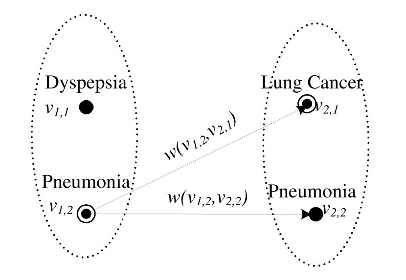
Figure 1: Julia’s $SUG$.Her actual sensitive value is represented by the circled dot.

The key idea of $SUG$ is to represent all the possible sensitive values and updates of a record in a graph: each node represents a possible sensitive value and each edge represents a feasible update on a sensitive value. We call an update $U(s_{s},s_{t})$ feasible only if sensitive value $s_{s}$ has non-zero probability update to $s_{t}$.

Suppose that before $T^{*}_{n+1}$ is released, $t^{{}^{\prime}}_{1},t^{{}^{\prime}}_{2},...,t^{{}^{\prime}}_{I}$ ($I\leq n$) are the sequential versions of record $t$ which exist in the corresponding releases of $T$. Formally, $t$’s $SUG$ is defined as follows:

Definition 10 (SUG).

Before $T^{*}_{n+1}$ released, $t$’s sensitive attribute update graph is denoted by $G_{n}(V,E)$, such that

• there is a one-to-one mapping between node $v_{i,j}$ ($v_{i,j}\in V$) and one possible sensitive value $s_{i,j}$ of $C_{i}$, where $i$ is any integer between $1$ and $I$.

• the weight of each node $v_{i,j}$ is the probability of an adversary linking $t^{{}^{\prime}}_{i}$ to $s_{i,j}$ only with the help of background knowledge ($BK_{i}-BK_{i-1}$).

• an edge $(v_{i,j},v_{i+1,k})$ represents a feasible update $U(s_{i,j},s_{i+1,k})$ and its weight $w(v_{i,j},v_{i+1,k})$ represents the probability of that feasible update happens, which is equal to $P_{trans}(s_{i,j},s_{i+1,k})$.

For a $SUG$, the weights of nodes and edges are determined by the background knowledge. Specifically, the weight of a node is the linking probability between $t$ and a sensitive candidate value without the help of historical background knowledge. That’s similar to the linking probability in the publication of static dataset. However, in dynamic dataset, the linking probability is determined together with the historical information hidden in the other parts of the graph.

It is apparent that a record’s candidate sensitive sets and their correlation are all encoded into a $SUG$. From the adversary’s perspective, $G_{n}(V,E)$ contains all the background knowledge about $t$’s sensitive information before $T^{*}_{n+1}$ released. Thus on the basis of $G_{n}(V,E)$, s/he can deduce the disclosure risk $r_{n}(t^{{}^{\prime}}_{i})$ for any integer $i$ between 1 and $I$.

Example 3.

Fig. 1 is Julia’s $SUG$ after Table I-A and I-A released. Without additional knowledge and specific declaration, we follow the random world assumption [7] that all the sensitive values in a sensitive candidate set have the equal linking probability, and the updates on a sensitive value have equal probability to happen. Thus the weight of every node and edge is 1/2 in fig. 1. The disclosure risk $r_{2}(t^{{}^{\prime}}_{1})$ is $100\%$ as $v_{1,1}$ has not outgoing edge; $r_{2}(t^{{}^{\prime}}_{2})$ is $50\%$ as both $v_{2,1}$ and $v_{2,2}$ has an incoming edge from $v_{1,2}$.

However, the $SUG$ can be further reduced by excluding some invalidate nodes and edges. E.g., in fig. 1, there’s no edge connect to $v_{1,1}$, that indicates dyspepsia can update to neither lung cancer nor pneumonia. Thus we know that Julia is impossible to contract dyspepsia and $v_{1,1}$ has no validate information. So we can deduce a subgraph only contains the validate information:

Definition 11 (feasible sub-$SUG$).

A feasible sub-$SUG$
$G^{\prime}_{n}(V^{\prime},E^{\prime})$ is a subgraph of $G_{n}(V,E)$ induced as follows:

Delete node $v$ and its connected edges from $G_{n}(V,E)$ if one of the following conditions holds:

• $v\in V_{1}$ and $deg^{-}(v)=0$;

• $v\in V_{I}$ and $deg^{+}(v)=0$;

• $v\in V_{i}$, $i\in(1,I)$, and at least $deg^{+}(v)=0$ or $deg^{-}(v)=0$ holds;

Repeat the process until no deletion left.

The above definition also provides a method to induce a feasible sub-$SUG$ from $SUG$. Actually, the deducing process is also the major part of the attack: excluding invalidate information so as to narrow the possible space of the sensitive values.

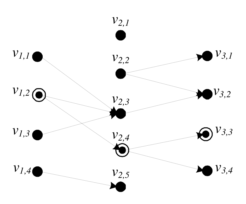
(a) A sample $SUG$

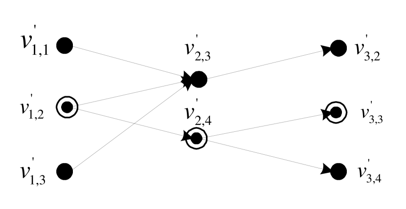
(b) A sample feasible sub-$SUG$

Figure 2: $SUG$

Fig. 2(b) is the feasible sub-$SUG$ deduced from fig. 2(a). As we observe, in a feasible sub-$SUG$, every path that begins from node in $V^{{}^{\prime}}_{1}$ and ends with node in $V^{{}^{\prime}}_{I}$ (we call it a feasible path) may represent the actual path that indicates the evolvement of $t$’s sensitive value. Thus at a specific time, once we get a record’s feasible sub-$SUG$, we can calculate the probability of each possible path, which can lead to the estimation of its disclosure risks $r_{n}(t^{{}^{\prime}}_{1}),r_{n}(t^{{}^{\prime}}_{2}),...,r_{n}(t^{{}^{\prime}}_{I})$.

III-B Disclosure Risk Estimation

The second part of the attack is the disclosure risk estimation. Since every path in the feasible sub-$SUG$ may be the one which contains all the correct sensitive values and updates, the weight portion of the feasible paths that crossing a node is just the probability that the correct path contains it, which is also the probability of linking $t^{{}^{\prime}}_{i}$ to the sensitive value represented by the node. Thus $r_{n}(t^{{}^{\prime}}_{i})$ equals to the weight portion of all the feasible paths that crossing the node representing $t^{{}^{\prime}}_{i}[S]$ in $V^{{}^{\prime}}_{i}$.

In order to calculate the risk, we first enumerate all the feasible paths by traversing $G^{\prime}_{n}(V^{{}^{\prime}},E^{{}^{\prime}})$. Then we compute the weight of every feasible path with the help of related nodes and edges. Assume $p_{k}=\{v^{{}^{\prime}}_{1,x_{1}},v^{{}^{\prime}}_{2,x_{2}},...,v^{{}^{\prime}}_{I,x_{I}}\}$ is any feasible path in $G^{\prime}_{n}(V^{{}^{\prime}},E^{{}^{\prime}})$, $v^{{}^{\prime}}_{i,x_{i}}$ is a node in $V^{{}^{\prime}}_{i}$. The weight of $p_{k}$ is the product of all the nodes and edges it traverses:

$$w(p_{k})=w(v^{{}^{\prime}}_{I,x_{I}})\prod^{I-1}_{i=1}w(v^{{}^{\prime}}_{i,x_{i}})w(v^{{}^{\prime}}_{i,x_{i}},v^{{}^{\prime}}_{i+1,x_{i+1}})$$ (1)

Finally, picking out all the feasible paths that crossing the node represents $t^{{}^{\prime}}_{i}[S]$, their portion equals to $r_{n}(t^{{}^{\prime}}_{i})$:

$$r_{n}(t^{{}^{\prime}}_{i})=\frac{\sum^{K_{i}}_{k^{{}^{\prime}}=1}w(p_{k^{{}^{\prime}}})}{\sum^{K}_{k=1}w(p_{k})}$$ (2)

$K$ is the total number of feasible paths and $K_{i}$ is the count of feasible paths that crossing the node represents $t^{{}^{\prime}}_{i}[S]$.

Example 4.

Consider the feasible sub-$SUG$ in fig. 2(b). There are totally 5 feasible paths in this graph. Enumerating them from top to down, their weights are 1/18, 1/36, 1/72, 1/72 and 1/18 respectively. The sum is 1/6.

There are 3 feasible paths crossing node $v^{{}^{\prime}}_{1,2}$: $\{v^{{}^{\prime}}_{1,2},v^{{}^{\prime}}_{2,3},v^{{}^{\prime}}_{3,2}\}$, $\{v^{{}^{\prime}}_{1,2},v^{{}^{\prime}}_{2,4},v^{{}^{\prime}}_{3,3}\}$ and $\{v^{{}^{\prime}}_{1,2},v^{{}^{\prime}}_{2,4},v^{{}^{\prime}}_{3,4}\}$. So $r_{3}(t^{{}^{\prime}}_{1})=(1/36+1/72+1/72)/(1/6)=1/3$. Similarly, we have $r_{3}(t^{{}^{\prime}}_{2})=1/6$ and $r_{3}(t^{{}^{\prime}}_{3})=1/12$.

We can estimate $r_{n}(t^{{}^{\prime}}_{1}),r_{n}(t^{{}^{\prime}}_{2}),...,r_{n}(t^{{}^{\prime}}_{I})$ based on $G^{{}^{\prime}}_{n}(V^{{}^{\prime}},E^{{}^{\prime}})$. Generally, for any positive integer $j$, in order to estimate $r_{j}(t^{{}^{\prime}}_{1}),r_{j}(t^{{}^{\prime}}_{2}),...,r_{j}(t^{{}^{\prime}}_{I})$, we should construct its feasible sub-$SUG$ $G^{\prime}_{j}(V^{{}^{\prime}},E^{{}^{\prime}})$ with the help of $BK_{j}$.

The increasing releases of $T$ will lead $t$’s feasible sub-$SUG$ dynamic and growing. Thus $r_{j}(t^{{}^{\prime}}_{i})$ is usually not equal to $r_{k}(t^{{}^{\prime}}_{i})$ ($j\neq k$). Because in $t$’s different feasible sub-$SUG$s, the weight portion of feasible paths that crossing the same node is usually variant. However, there are still exceptions:

Lemma 1.

If all the sensitive values in the sensitive domain can randomly updated to any other value (including itself), the disclosure risks of the existing sensitive information are invariant regardless how to release the new publications.

Proof.

The proof of lemmas can be found in [8].

The lemma also implies the anonymization problem of dynamic dataset can be reduced to several independent anonymization problem of static dataset when the internal updates on sensitive values are totally random. Because the random updates of sensitive values lead different publications to no correlation: $T_{n}$ and $T_{n+1}$ are entirely independent.

Generally, we have the following lemma for dynamic dataset which theoretically demonstrates at what time the disclosure of sensitive information happens:

Lemma 2.

Regardless how to publish the dataset, for any positive integer $i$ and $n$ ($i\leq n$), $r_{n}(t^{{}^{\prime}}_{i})=1$ holds iff $|V^{{}^{\prime}}_{i}|=1$ holds in the corresponding feasible sub-$SUG$.

III-C $SUG$ Applicability Demonstration

As mentioned, $SUG$ is a general privacy disclosure framework for re-publication problem. Exploiting it to analysis any re-publication problem, we follow two steps:

1. Constructing the record’s $SUG$ and deducing the corresponding feasible sub-$SUG$;

2. Calculating the weight of each feasible path and estimating disclosure risks.

Let us apply the framework to re-publish external dynamic dataset [4]. Since there is no internal update in the external dynamic dataset, each node have at most one incoming edge and one outgoing edge in a record’s $SUG$; each edge connects two nodes which represent the same sensitive value. After excluding the invalidate information in the $SUG$, the feasible sub-$SUG$ must have the following characteristics:

1. For each feasible path, all the nodes it crossed represent the same sensitive value;

2. For each node, there is only one feasible path crossing it.

Intuitively, the feasible sub-$SUG$ contains several parallel feasible paths and each one contains the same sensitive value. According to lemma 2, the disclosure will occur when there is only one feasible path left. The analysis also hints us that, if we can guarantee that the feasible sub-$SUG$ always have several indistinguishable feasible paths, the disclosure will not happen. Moreover, employing our estimation method, we will get that the re-publication risk of m-Invariance is $1/m$ as each feasible path has equal weight.

The analysis above also convinced us that re-publication of external dynamic dataset is a special case of our problem. Revisiting fully dynamic dataset, as illustrated in fig. 2(b), the $SUG$ of each record is more complex and the risks are difficult to control. However, if we can make a similar guarantee: in each record’s feasible sub-$SUG$, there always exists several indistinguishable feasible paths and each candidate node set contains several nodes, at least the disclosure will not occur.

IV Anonymization Principle

According to the analysis in the previous section, if a record’s sensitive information is well protected in each separate publication, the disclosure is mainly rose by the pruning to its $SUG$. In other words, if we prevent the possible pruning to the record’s $SUG$ and always guarantee $|V^{{}^{\prime}}_{i}|>1$ for all $i$, the disclosure of sensitive information will never happen.

Referring to a dataset containing a mount of records, we should pay more attention: when publishing the dataset, we need guarantee that there will be no pruning to all the records at any time, as to prevent the chain-actions of disclosure [6].

Specifically, two requirements need to be met:

1. All the records’ sensitive information is well preserved in each separate publication;

2. At any time, there is no pruning to all the records’ $SUG$ so as to maintain the indistinguishability of sensitive values.

In this paper, we use m-unique [4] to illustrate the sensitive value indistinguishability: if there are at least m records in $QI$-group $g$ and all of them have distinct sensitive values, we call $g$ is m-unique; a published table is m-unique if all the $QI$-groups in it are m-unique.

IV-A m-Distinct

Before presenting our method, we formulate the following concept to describe the update candidates of a value:

Definition 12 (Candidate Update Set).

Suppose $a$ is an element in the domain of attribute $\mathcal{A}$ ($a\in dom(\mathcal{A})$), its candidate update set $CUS(a)$ is the union of some elements in $dom(\mathcal{A})$, such that $a$ has non-zero update probability to it.

Note that if $b\in CUS(a)$, then $CUS(b)\subseteq CUS(a)$ must hold. Similarly, we have the following notion for a group of sensitive values:

Definition 13 (Update Set Signature).

Suppose $QI$-group $g$ contains $n$ records and their sensitive values are $s_{1},s_{2},...,s_{n}$, respectively. Then $g$’s update set signature $USS(g)$ is a multi-set: {$CUS(s_{1}),CUS(s_{2}),...,CUS(s_{n})$}.

Since $USS$ is a multi-set of $CUS$, the same $CUS$ may appear several times in a $USS$, because several records may have the same sensitive value and different sensitive values may even have the equal candidate update set. Record $t$’s update set signature, which is inherited from the $QI$-group it is in, is denoted by $USS(t)$. It is obvious that a record’s $USS$ is dynamic as the re-publication progress evolves, because in different time the sensitive values of its $QI$-group are variant.

In this paper, we say that $USS_{i}$ and $USS_{j}$ ($i\not=j$) are intersectable, if they have equal number of $CUS$ and there exists a one-to-one map between two $CUS$ in $USS_{i}$ and $USS_{j}$, such that the intersection of the two $CUS$ is non-empty; moreover, if the $CUS$ of $USS_{j}$ is a subset of the $CUS$ of $USS_{i}$, we call $USS_{i}$ implies $USS_{j}$ (denote as $USS_{i}\supseteq USS_{j}$).

Next, we explains under what conditions, a set of values is a legal update instances of a $USS$:

Definition 14 (Legal Update Instance).

A set of sensitive values $S=\{s_{1},s_{2},...,s_{n}\}$ is a legal update instance of a $USS$ if the following conditions hold:

1. The number of sensitive values in $S$ equals to the number of $CUS$ in the $USS$: $|S|=|USS|$.

2. For any value $s_{i}$ in $S$, there is at least one candidate update set $CUS_{j}$ such that $s_{i}\in CUS_{j}$.

3. For any candidate update set $CUS_{j}$ in $USS$, there is at least one sensitive value $s_{i}$ in $S$ such that $s_{i}\in CUS_{j}$.

If a group of sensitive values are a legal update instance of a $USS$, in the perspective of adversary, every value in it can not be excluded. Suppose $t$’s candidate sensitive set $C$ is a legal update instance of its $USS$ in the previous publication, then the deduce procedure (as illustrated in section III-A) can not exclude any node or edge: all the information in its $SUG$ are validate. Hence the threats rose by invalidate information exclusion are prevented.

Example 5.

In the example of section I-B, Julia’s candidate sensitive set $C_{1}$ is $\{Dyspepsia,Pneumonia\}$. With the help of implicit background knowledge, we know that
$CUS(Dyspepsia)=\{Dyspepsia,Gastritis,other\;digestive\;\\ system\;diseases\}$ and $CUS(Pneumonia)=\\ \{Pneumonia,Flu,Lung\;Cancer,other\;respiratory\;\\ system\;diseases\}$. Thus Julia’s update set signature in the $1^{st}$ release is $\{CUS(Dyspepsia),CUS(Pneumonia)\}$.

According to definition 14, if we randomly pick out an element from $CUS(Dyspepsia)$ and $CUS(Pneumonia)$ respectively, then the two elements must be a legal instance of $USS(Julia_{1})$.

Now we are ready for our anonymization principle:

Definition 15 (m-Distinct).

$T$ is a dynamic dataset, a sequential releases of $T$: $T^{*}_{1},T^{*}_{2}$, $T^{*}_{3}$, $...$, $T^{*}_{n}$ are m-Distinct if it meets:

1. For all $i\in[1,n]$, $T^{*}_{i}$ is m-unique.

2. Suppose for any record $t$, $T_{i}$ and $T_{j}$ ($i<j$) are two neighboring releases which both contain $t$ ($t_{i}\in T_{i}$, $t_{j}\in T_{j}$). For all $i\in[1,n]$, $t_{j}$’s candidate sensitive set $C_{j}$ is a legal update instance of $USS(t_{i})$.

The rationale of m-Distinct is that, we adopt m-unique to maintain the indistinguishability of sensitive values in each separate publication; then when releasing new publication, we carefully partition the records so that the indistinguishability of sensitive values is still maintained. In other words, the concept of “legal update instance” guarantees that there is no inference rose by information exclusion.

Revisit example 5, since Julia’s candidate sensitive set $C_{2}$=$\{Dyspepsia,Lung\;Cancer\}$ is a legal update instance of $\{CUS(Dyspepsia),CUS(Pneumonia)\}$, $T^{*}_{1}$ and $T^{*}_{2}$ are 2-Distinct with respect to Julia.

Deriving from definition 15, when releasing a new version of $T$ and maintaining the m-Distinct property meanwhile, we only need the information of most recent versions of the records. Specifically, if the two following conditions hold:

1. the new version $T^{*}_{new}$ is m-unique;

2. for any record $t$ ($t_{new}\in T_{new}$), suppose $t_{pre}$ is $t$’s most recent version, then $t_{new}$’s candidate sensitive set is a legal update instance of $USS(t_{pre})$.

Then the sequential release including $T^{*}_{new}$ are also m-Distinct. Furthermore, we have the following lemma:

Lemma 3.

If a sequential releases of $T$: $T^{*}_{1},T^{*}_{2}$, $T^{*}_{3}$, $...$, $T^{*}_{n}$ are m-Distinct, then for any record $t\in T$, $|V^{{}^{\prime}}_{i}|\geq m$ holds for all the candidate node sets in its feasible sub-$SUG$ $G^{\prime}_{n}(V^{\prime},E^{\prime})$.

Lemma 3 reveals that the disclosure will not occur if the releases are m-Distinct. A larger $m$ usually makes the disclosure more difficult because more values are indistinguishable in each QI-group.

IV-B m-Distinct Extension

m-Distinct guarantees that no disclosure of sensitive values will occur, however, sometimes more strict anonymization principle may be needed to limit the re-publication risk. Thus we have the following principle called m-Distinct^∗:

1. the requirements of m-Distinct hold.

2. Suppose for any record $t$, $T_{first}$ is the first release contains $t$ ($t_{first}\in T_{first}$). then $CUS_{\alpha}\cap CUS_{\beta}=\phi$ ($\alpha\neq\beta$) holds for any two candidate update sets in $USS(t_{first})$.

Then the following consequence holds:

Lemma 4.

If a sequential releases of $T$: $T^{*}_{1},T^{*}_{2}$, $T^{*}_{3}$, $...$, $T^{*}_{n}$ are m-Distinct^∗, then the re-publication risk is at most $1/m$.

The key of m-Distinct^∗ is the $2^{nd}$ condition. It implies that, in the same $QI$-group, every sensitive value’s $CUS$ does not overlap with the other values’.

By applying our privacy disclosure framework, m-Distinct^∗ can limit the re-publication risk to $1/m$ because it guarantees that there are at least $m$ parallel feasible paths in every record’s feasible sub-$SUG$. However, m-Distinct^∗ may not be met in general case: there may not exist $m$ sensitive values to form a QI-group in which there is no overlap between the $CUS$ of any two sensitive values.

V Algorithm

We now present an algorithm to meet m-Distinct. According to the analysis in previous section, if every new release of the dataset meets the two conditions in previous section, then m-Distinct persists in the sequential release. Thus we put the attention on releasing $T^{*}_{n}$ based on the previous releases.

When anonymizing $T_{n}$, the crucial part of maintaining m-Distinct property is that, every record’s new candidate sensitive set should be a legal update instance of its previous $USS$. The basic idea of our algorithm is to assign records to proper bucket according to their $USS$ such that we can always find a way to partition records into $QI$-group, of which the candidate sensitive set is a legal update instance of these records. The overview of our algorithm is described in Algorithm 1.

Algorithm 1 Overview of Our Algorithm

0:  $T_{n}$: the $n^{th}$ version of $T$; $m$: the user configured parameter for m-Distinct; $t_{pre}$: the most recent version of $t$, where $t\in T_{n}$ and $t$ has appeared in $T$ before;

1:  create buckets $Q_{buc}$ according to the records which has $t_{pre}$;

2:  assign records to proper position of proper bucket in $Q_{buc}$;

3:  partition the unassigned records into m-unique $QI$-groups;

4:  recursively split each bucket into two until no more split left (forms $QI$-groups);

5:  generalize each $QI$-group;

6:  publish the generalized $QI$-groups and counterfeit statistics.

In our algorithm we introduce counterfeit records when no enough record in the dataset helps to meet m-Distinct. Note that the only usage of the counterfeit records is to maintain the sensitive value indistinguishability of a $QI$-group.

Except for meeting the anonymization principle, we also aims to minimize two criterions: the number of counterfeit records and the generalization of $QI$ attributes. Because more counterfeit records will cover up more characteristics of the original dataset and more generalization will lead to more information loss, both are harm to the dataset utility.

Our algorithm mainly contains the three following phases.

V-A Phase 1: Creating Buckets

Algorithm 2 Create Buckets

0:  $Q_{rec}$: the queue of records in $T_{n}$; $t_{pre}$: the most recent version of $t$, where $t\in T_{n}$ and $t$ has appeared in $T$ before;

1:  Let $Q_{buc}$ and $Q_{tmp}$ be empty queues of buckets;

2:  for all record $t$ in $Q_{rec}$ do

3:     if $t_{pre}$ exists then

4:        create $B_{new}$ such that $USS(B_{new})=USS(t_{pre})$;

5:        if $B_{new}$ does not exist in $Q_{buc}$ then

6:           enqueue($Q_{buc},B_{new}$);

7:  for every 2 buckets $B_{i},B_{j}\in Q_{buc}(i<j)$ do

8:     if $USS(B_{i})$ and $USS(B_{j})$ are intersectable then

9:        pick out their highest scored intersection plan $USS_{new}$;

10:        create $B_{new}$ such that $USS(B_{new})=USS_{new}$;

11:        if $B_{new}$ does not exist in $Q_{buc}$ and $Q_{tmp}$ then

12:           enqueue($Q_{tmp},B_{new}$);

13:  append($Q_{buc},Q_{tmp}$);

14:  return $Q_{buc}$;

Our algorithm (algorithm 2) will first create buckets which the records are possibly in. Note that a bucket is only identified by its $USS$.

Suppose for any record $t\in T_{n}$, $t_{pre}$ is $t$’s most recent version. First, we create a bucket $B_{new}$ for $t$, such that $USS(B_{new})$ equals to $USS(t_{pre})$ (lines 2-6). We only skip record $t$ if such bucket is already exist, or this is the first time $t$ appears in the dataset. We denote an entry of bucket $B$ as a candidate update set in $USS(B)$. The number of entries equals to the number of candidate update sets of $B$.

In the second step (lines 7-12), we generate new bucket based on the buckets created in the previous step: if any two buckets are intersectable, we create a new bucket whose update set signature is the intersection of their $USS$; if there are several possible intersection plans, we choose the one with highest score: the higher proportion of the overlapped elements, the higher score of the intersection plan.

At the end of this phase, we have all the possible buckets for the records of $T_{n}$ which have appeared before. For the new records, we will create new bucket for them later, if no existing bucket is suitable.

V-B Phase 2: Assigning Records

Algorithm 3 Assign Records

0:  $Q_{rec}$: the queue of sorted records ($CNT_{buc}\geq 1$ for all); $CNT_{buc}(t)$: the number of buckets $t$ can be assigned; $Q_{t}$: the queue of suitable buckets for record $t$.

1:  while $Q_{rec}$ is not empty do

2:     $t\leftarrow$dequeue($Q_{rec}$);

3:     max_score$\leftarrow-\infty$;{global maximum score of $t$}

4:     while $Q_{t}$ is not empty do

5:        $B\leftarrow$dequeue($Q_{t}$);

6:        buc_score$\leftarrow-\infty$;{maximum score of $t$’s assignment in $B$}

7:        for entry $e_{i}$ in $B$ do

8:           if $t[S]\in e_{i}$ then

9:              tmp_score$\leftarrow$get_score($t,B,e_{i}$);

10:              if tmp_score==buc_score then

11:                 buc_entry$\leftarrow$choose_entry(buc_entry, $i$);

12:              else if tmp_score$>$buc_score then

13:                 buc_score$\leftarrow$tmp_score;

14:                 buc_entry$\leftarrow$$i$;

15:        if buc_score$>$max_score then

16:           max_score$\leftarrow$buc_score;

17:           max_entry$\leftarrow$buc_entry;

18:           max_buc$\leftarrow B$;

19:     assign($t$,max_buc, max_entry);

The main task of this phase is to assign records to proper bucket and the corresponding entry. If record $t$ and bucket $B$ meet $USS(t_{pre})\supseteq USS(B)$ and $t[S]$ is covered by $USS(B)$, then $t$ can be assigned to $B$. The reason is that, when we pick out an record from each entry of the bucket and forms a $QI$-group (will carry on in next phase), if there is no duplicate sensitive value in the group, the $QI$-group must hold m-Distinct. Because the candidate sensitive set of $t$ now must be a legal update instance of $USS(B)$ as well as $USS(t_{pre})$.

Referring to a record which appears in the dataset the first time, it can be assign to a bucket only if its current sensitive value is covered by the bucket’s $USS$.

In order to facilitate the task, we first calculate $CNT_{buc}(t)$, the number of buckets $t$ can be assigned, and sort the records increasingly according to their $CNT_{buc}$.

The records which have no existing buckets to be assigned in ($CNT_{buc}$=0), must also be the first time appears in the dataset. Thus we process them separately: partitioning them into $QI$-groups which are m-unique. It can be done by exploiting existing anonymization algorithms [9, 10, 4] because they have no previous version involved. Note that counterfeit records will be added in case they are not m-eligible.

The rest of the records, which can be assigned to at least one bucket, will be assigned to a bucket sequentially as algorithm 3. Since there are $K!$ (denote $K$ as the number of rest records) orders to assign these records, our greed algorithm starts the assignment by processing the records with least $CNT_{buc}$, because they have less optional buckets and can be determined with less overheads.

In algorithm 3, we consider each possible bucket (line 4) and entry for a record so as to get the highest scored assignment. A record $t$ can be assigned to an entry $e_{i}$ only if the $CUS$ it represented contains $t[S]$ (line 8). Specifically, the score of $t$ with respect to $e_{i}$ of $B$ (line 9) is calculated as follows:

(i) We define $\epsilon$ to indicate $t$’s contribution to counterfeit counts if $t$ is assigned to $e_{i}$. $\epsilon=1$ means $t$’s assignment will not increase the counterfeit count in $B$; otherwise, $\epsilon$ is $-1$. So we first calculate parameter $\delta$, such that $\delta=max\{F_{max},|e_{1}|,|e_{2}|,...,|e_{|USS(B)|}|\}$, where $F_{max}$ is the maximal frequency of sensitive value in $B$. Then we set $\epsilon$ to be $-1$ if the frequency of $t[S]$ in $B$ equals $\delta$ or $|e_{i}|$ equals $\delta$.

(ii) We also define a parameter to indicate $t$’s contribution to the further generation: $\lambda=Z_{aft}/Z_{bef}$. $Z_{bef}$ and $Z_{aft}$ are the $|QI|$-dimensional area generated by all the records in $B$ before and after $t$’s assignment. Apparently, $\lambda\geq 1$ and a larger value indicates $t$’s assignment brings into more generation.

(iii) At last we return the following score:

$$score=\left\{\begin{array}[]{ll}1/\lambda&if\;\epsilon=1\\ -\lambda&if\;\epsilon=-1\end{array}\right.$$ (3)

The above equation blends $t$’s contributions to counterfeit count and generalization together. Obviously, a larger score of $t$’s assignment shows that it will bring into less counterfeit records and generalization.

When two entries in $B$ has the same score, we assign the record into the entry with less already assigned records (line 11 choose_entry), so as to get a more balanced bucket. Once we get the assignment with least score, we immediately assign this record to the bucket by pushing it into the corresponding bucket entry (line 19).

After all the records are assigned, the buckets will be balanced with counterfeit records so as they are m-eligible. Thus we calculate $\delta$ as before, then add counterfeit records to the entries so that each entry has $\delta$ records.

V-C Phase 3: Generating $QI$-groups

Now every bucket is m-eligible and is well prepared for generating $QI$-groups. Since there are $|USS(B)|$ entries in $B$ and each one has $\delta$ records, it is workable to split the bucket into $\delta$ $QI$-groups: each one contains only one record of an entry and all the records have distinct sensitive values.

In this phase, we will recursively split each bucket into two children until only one record left in each entry. In order to perform further split on the generated buckets, the child buckets should also be m-eligible. Specifically, both of them should meet the following conditions:

1. balanced;

2. $F_{max}$ should not be larger than the number of records in each entry.

Besides, in order to generate $QI$-groups with least information loss, each split we aims to minimize the generalization. Similar to [4], we calculate score for a split plan as follows:

$$split\_score=\sum^{2}_{i=1}(|B_{i}|\cdot\sum^{d}_{j=1}\frac{l_{i,j}}{I_{j}})$$ (4)

where $l_{i,j}$ and $I_{j}$ are the minimum interval of attribute $q_{j}$ in $B_{i}$ and $B$, respectively.

To find the split plan with least score, we organize the records of a bucket in a queue and sort them according to attribute $q_{i}$. Then we greedily pick out records from the queue so as to form two child buckets. The split plan with least score is kept. After we do the above procedure for all the $QI$ attributes, we choose the minimum one and apply it to $B$.

The key of this phase is how to pick out records so as to form two child buckets which both meet the above conditions. In our algorithm, each time we traversal the queue and pick out $|USS(B)|$ records, which are all from different entries and have no duplicate sensitive value. The pick-out procedure executes recursively so as to pick out more records and generate all the possible split plans. In the worst case, ${\delta^{{}^{\prime}}}^{|USS(B)|-1}$ operations may be performed in order to pick out $|USS(B)|$ legal records. $\delta^{{}^{\prime}}$ is the current number of records which are still left in each entry.

Note that if $B$ can not be split again and it has counterfeit record in entry $e_{i}$, we will randomly assign the counterfeit record a sensitive value, which is pick out from the $CUS$ that $e_{i}$ represented and different from the existing values in $B$.

At last, we generalize all the $QI$-groups formed in phase 2 and 3 and publish them together with the corresponding counterfeit statistics.

V-D Extension

The presented algorithm is a general method to meet m-Distinct. According to the definition of m-Distinct^∗, it has an additional constrain on the $1^{st}$ release of any record in contrast to m-Distinct. Thus we only need to handle the $QI$-group with new records particularly: grantees that it has at least m records with different sensitive values and the $CUS$ of any two records’ sensitive values are not overlapped.

To achieving this, in each publication, we will first check whether there are suitable buckets created in phase 1 for the new record. The record will be assigned in if such a bucket found, otherwise we partitioning these new record into new $QI$-groups as did in the anonymization of static dataset but with an addition criterion: in each $QI$-group, no overlap exists between any two sensitive values’ $CUS$. For the old records, we process them no difference to the procedure in m-Distinct.

VI Experiments

The experiments were performed on a 3GHz Intel IV processor machine with 2GB memory. All the algorithms are implemented in C++.

VI-A Experiment Setup

We use a real dataset OCC from http://ipums.org, which is also adopted by [3, 4]. The dataset consists of 200k records with four $QI$ attributes and one sensitive attribute. More detail information of the dataset is given in table VII. Vital parameters of the experiment are set as follows:

External Update. Since the external update property is well investigated in [4], in our experiment, we use a fixed external update rate: we began to publish $T_{1}$ with 20,000 records which are randomly chose from the original dataset; then in each new release $T_{i}$, we randomly remove 2,000 records from $T_{i-1}$ and insert 5,000 records from the rest of records. The dataset will be re-published 20 times.

Internal Update. As no existing dataset contains internal updates information explicitly, we generate internal updates according to the semantic of each attribute. In the span of $[i,i+1]$, the internal updates are configured as follows:

• Age: the age of each record will increase 1 till reach 100;

• Gender: will not change;

• Marital Status/ Education: will update according to the specific semantic of each value. E.g., the marital status of a record may update from married to any one in {married, divorced, separated, widowed} but can not update to be never-married; its education may update from bachelor to any eduction not lower than bachelor.

• Occupation: since the internal update on sensitive attribute is critical to the problem of this paper, we introduce internal update diameter d to describe the flexibility of internal updates on sensitive attribute. An sensitive value’s d equals to the size of its candidate set. Apparently, a large diameter indicates more flexible internal updates.

  By default, we set $d$ to be 10, which means a person’s occupation may stay the same or change to be nine other similar jobs with equal probabilities. Noticing that in each publication, we set the internal updates on sensitive values only randomly occurred on 5,000 records.

TABLE VII: Dataset Description

attribute	Age	Gender	Marital.	Education	Occupation
dom. size	100	2	6	17	50
type	num.	cat.	cat.	cat.	cat.

VI-B Invalidation of Existing methods

We first perform experiments to show the inadequacy of the existing anonymization methods.

The l-diversity algorithm in [10] is exploited to re-publish the dynamic dataset. Fig. 3(a) demonstrates the total number of vulnerable sensitive values if the dataset is re-published using l-diversity. Note that there are $n$ versions of sensitive value related to a record if it is published $n$ times. The result confirms that l-diversity is insufficient to re-publish dynamic dataset, e.g. about $66\%$ percentage of the published sensitive values are disclosed when the dataset is published 20 times using $2$-diversity. Although a larger $l$ will lead less disclosure, the number of disclosed sensitive values increases as the re-publication process evolves.

We also test the number of vulnerable sensitive values versus internal update diameter (fig. 3(b)). A smaller diameter usually leads to more vulnerable sensitive information, because the updates on sensitive values are less flexible and more pruning will be performed when deducing the feasible sub-$SUG$. Besides, the total vulnerable information decreases as $l$ grows, because lemma 2 is more difficult to be met when more records are plunged into a group.

In the next experiment, we show the invalidation of m-Invariance. We adopt the algorithm in [4] to re-publish dataset and report the total number of invalidate records. As expected, the invalidate counts increase gradually as new publication releases (fig. 4(a)).

Since the invalidation of m-Invariance is cause by internal updates, we test the invalidate record counts with respect to the diameter (fig. 4(b)).The invalidate counts increase dramatically with respect to the increase of diameter. Specially, when the diameter is 1, which means each value can not update to be anyone else, there is no invalidate records. That reconfirmed that the invalidation reason of m-Invariance is internal update.

(a) Vs. time

(b) Vs. d

Figure 3: Total vulnerable counts

(a) Vs. time

(b) Vs. d

Figure 4: Number of invalidate records

VI-C m-Distinct Evaluation

In this subsection, we will evaluate our solution from the following aspects:

VI-C1 Query Accuracy

We test the query accuracy of anonymization data by answering aggregate queries as follows:

SELECT COUNT(*)
FROM $T_{i}$
WHERE	$Q_{1}>a_{1}$	AND $Q_{1}<b_{1}$
		…
	$Q_{4}>a_{4}$	AND $Q_{4}<b_{4}$
	$S>a_{5}$	AND $S<b_{5}$

For each query, we configure its range as $|b_{j}-a_{j}|=\theta\cdot|dom(A_{j})|$, where $\theta\in(0,1]$. Apparently, a query with larger $\theta$ will involve more records and return a larger result.

The query error, which is the difference between the returned results on $T_{i}$ and $T^{*}_{i}$, is $|R^{*}-R|/R^{*}$. $R$ is the query result on $T_{i}$ and $R^{*}$ is the estimated result on $T^{*}_{i}$. Specifically, the estimated result is the number of possible records which are in QI-group $g$ and covered by the query. Suppose the records in $g$ are uniformly distributed, the probability of a record $t$ meets the query is the product of probabilities that $t[A_{j}]$ ($i=1,2,...,5$) is in the interval $(a_{j},b_{j})$. Thus $R^{*}$ equals to the product of the records count of $g$ (excluding counterfeit counts) and the above probability.

In this experiment, we randomly generate 10,000 queries and report the median error. Fig. 5(a) shows the median errors for different time and m. The median error increases smoothly as time evolves, because the new inserted records for a QI-group are usually not as ’well’ as the deleted ones; however, as the result of 2(4)-Distinct demonstrated, the median error will not increase anymore when re-publishing enough times.

Fig. 5(b) shows the median error versus different $\theta$ while $m=4$. As expected, the query with larger range gets more accurate result, because when it covers more records, the estimation are more close to the actual result. At last, in fig. 7 we show the median error for different internal update diameter. Since a larger diameter means more flexible internal updates, which allows more records to be assigned in a bucket and is more flexible to generate QI-groups, the accuracy increases with $d$.

(a) Vs. time ($\theta=50\%$)

(b) Vs. $\theta$ ($m=4$)

Figure 5: Query error

Figure 6: Query error Vs. d ($m=4,\theta=50\%$)

Figure 7: $CNT_{g}$ Vs. time ($m=6,d=5$)

VI-C2 Counterfeit Counts

In this experiment we temporarily configure the delete amount of each re-publication to be 3,000 because our initial setup leads to zero counterfeit count in most of evaluations. We define the measurement as the average counterfeit count per QI-group (denote as $CNT_{g}$).

Fig. 7 plots the $CNT_{g}$ versus time when $m=6$ and $d=5$. $CNT_{g}$ increases at the beginning because more existing QI-groups have records been removed, that leads to a more urgency of counterfeit records in the balance step. However, after the $7^{th}$ publication, $CNT_{g}$ decreases as the total number of counterfeit records becomes more and more stabilized and the number of QI-groups are always increasing.

Then we fix $m=6$ and show the average $CNT_{g}$ per time with different configuration of d (fig. 8(a)). It is expected that a larger diameter makes the publication with less counterfeit records in each group, because it also means more flexible assignment for the inserted records.

In fig. 8(b) we set $d=5$ and measure the average $CNT_{g}$ per time for different m-Distinct. The result of 8-Distinct is the largest but also smaller than 2.

VI-C3 Computation Cost

According to the experiment setup, the number of re-publication records is incremental as time evolves. In order to accurately measure the cost of a single re-publication procedure, we report the average running time for re-publishing $T^{*}_{2}$.

Fig. 9(a) demonstrates the computation cost with different internal update diameter. A larger diameter can lead to higher data utility (fig. 7) as well as always needs higher cost. Because in phase 2, there may be more optional buckets for a new inserted records and more records will be assigned in the same bucket, which will lead to more cost when splitting and generating $QI$-groups in the last phase.

We also observe the cost comparing to different m. The cost decreases from 2 to 4 because a smaller m has less number of buckets and each bucket has more records, which need more split operations to generate $QI$-groups. However, the overhead increases from 4 to 8, that is because when m becomes larger, the major cost is how to find a legal split for a bucket with least information loss, which is positively correlated to m (as the analysis in section V-C).

(a) Vs. d ($m=6$)

(b) Vs. m ($d=5$)

Figure 8: average $CNT_{g}$ per time

VII Related Work

Most existing anonymization work is carried out on static datasets, where records are inserted and/or deleted dynamically. Different anonymization principles [2, 3, 10, 11, 12, 13] have been proposed to preserve privacy and ensure the sensitive information security from different perspectives. In addition to resisting different kinds of disclosure attacks [6, 10, 14, 15], the anonymization principles also struggle to achieve privacy preservation with less information loss. Many algorithms [1, 9, 14, 16, 17] have are also been proposed to generalize datasets to meet the principles with little overhead.

Relatively, the data re-publication has received less attention. Wang and Fung [18] first studied the problem of securely releasing multi-shots of a static dataset. The main challenge is the inference caused by joining between multiple releases. They proposed a solution to properly anonymize the current release so as to control possible inferences.

The anonymization work on dynamic datasets was initiated in  [5]. Byun et al. tackled the problem of incremental dataset anonymization, where a dataset is updated by only record insertion. Their solution supports neither record deletion nor attribute value update.

Xiao and Tao [4] first conducted anonymization on external dynamic datasets, which are updated by both record insertion and deletion. The challenge lies in that the inserted and deleted records may cause the disclosure risk of both themselves and the remained records, and even lead to the disclosure of individuals’ sensitive values. Their solution, called m-Invariance [4, 19], guarantees that each time the QI-group to which a record belongs contains the same set of sensitive values.

In short, all existing work do not consider internal updates, and their solutions are invalid for fully dynamic datasets. This constitutes the task for our paper to solve.

(a) Vs. d ($m=4$)

(b) Vs. m

Figure 9: Computation cost

VIII Conclusion

This paper challenges a new problem—enabling anonymization of dynamic datasets with both internal updates and external updates. For this goal, a novel privacy disclosure framework, which is applicable to all dynamic scenarios, is proposed. A new anonymization principle m-Distinct and corresponding algorithm are presented for anonymous re-publication of fully dynamic datasets. Extensive experiments conducted on real world data demonstrate the effectiveness of the proposed solution.

APPENDIX

Proof of lemma 1. Suppose $t^{{}^{\prime}}_{1},t^{{}^{\prime}}_{2},...,t^{{}^{\prime}}_{I}$ are the sequential versions of record $t$ which exist in the corresponding releases of $T^{{}^{\prime}}$. For any $1\leq i\leq I$, we have $t^{{}^{\prime}}_{i}\in T^{{}^{\prime}}_{i}$. Regardless how to release $T^{{}^{\prime}}_{I+1}$, if we can prove $r_{I}(t^{{}^{\prime}}_{i})=r_{I+1}(t^{{}^{\prime}}_{i})$ holds for any $1\leq i\leq I$, lemma 1 must holds.

Derive from the condition presented in the lemma, we know that $t$’s feasible sub-$SUG$ $G^{{}^{\prime}}_{I+1}(V^{{}^{\prime}},E^{{}^{\prime}})$ can be constructed on the basis of $G^{{}^{\prime}}_{I}(V^{{}^{\prime}},E^{{}^{\prime}})$: add $|C_{I+1}|$ nodes which represent the sensitive candidate set $C_{I+1}$ and draw edges from every node in the last sensitive candidate set of $G^{{}^{\prime}}_{I}(V^{{}^{\prime}},E^{{}^{\prime}})$ to every new node.

Suppose $p^{{}^{\prime}}_{k}$ is any feasible path in $G^{{}^{\prime}}_{I+1}(V^{{}^{\prime}},E^{{}^{\prime}})$, its weight can be represented as $w(p^{{}^{\prime}}_{k})=w(p_{k})w(v^{{}^{\prime}}_{I,x_{I}},v^{{}^{\prime}}_{I+1,x_{I+1}})w(v^{{}^{\prime}}_{I+1,x_{I+1}})=\frac{1}{|C_{I+1}|}w(p_{k})w(v^{{}^{\prime}}_{I+1,x_{I+1}})$, where $p_{k}$ is a feasible path in $G^{{}^{\prime}}_{I}(V^{{}^{\prime}},E^{{}^{\prime}})$ and contained by $p^{{}^{\prime}}_{k}$; node $v^{{}^{\prime}}_{I,x_{I}}$ and $v^{{}^{\prime}}_{I+1,x_{I+1}}$ are in $V^{{}^{\prime}}_{I}$ and $V^{{}^{\prime}}_{I+1}$ respectively and crossed by $p^{{}^{\prime}}_{k}$.

According to equation 2, we have $r_{I}(t^{{}^{\prime}}_{i})=\frac{\sum^{K_{i}}_{k^{{}^{\prime}}=1}w(p_{k^{{}^{\prime}}})}{\sum^{K}_{k=1}w(p_{k})}$. Similarly, we have $r_{I+1}(t^{{}^{\prime}}_{i})=\frac{\sum^{K_{i}\cdot|C_{I+1}|}_{k^{{}^{\prime}}=1}w(p^{{}^{\prime}}_{k^{{}^{\prime}}})}{\sum^{K\cdot|C_{I+1}|}_{k=1}w(p^{{}^{\prime}}_{k})}$. According to the construction process stated above, in $G^{{}^{\prime}}_{I+1}(V^{{}^{\prime}},E^{{}^{\prime}})$, the number of total feasible paths ($t^{{}^{\prime}}_{i}$ related feasible paths) are $|C_{I+1}|$ times of the count in $G^{{}^{\prime}}_{I}(V^{{}^{\prime}},E^{{}^{\prime}})$. Collaborate $r_{I+1}(t^{{}^{\prime}}_{i})$ with $p^{{}^{\prime}}_{k}$, we have $r_{I+1}(t^{{}^{\prime}}_{i})=\frac{\sum^{|C_{I+1}|}_{m^{{}^{\prime}}=1}\sum^{K_{i}}_{k^{{}^{\prime}}=1}w(p_{k^{{}^{\prime}}})w(v^{{}^{\prime}}_{I+1,x_{m^{{}^{\prime}}}})}{\sum^{|C_{I+1}|}_{m=1}\sum^{K_{i}}_{k=1}w(p_{k})w(v^{{}^{\prime}}_{I+1,x_{m}})}\\ =\frac{\sum^{K_{i}}_{k^{{}^{\prime}}=1}\{w(p_{k^{{}^{\prime}}})\sum^{|C_{I+1}|}_{m^{{}^{\prime}}=1}w(v^{{}^{\prime}}_{I+1,x_{m^{{}^{\prime}}}})\}}{\sum^{K_{i}}_{k=1}\{w(p_{k})\sum^{|C_{I+1}|}_{m=1}w(v^{{}^{\prime}}_{I+1,x_{m}})\}}$.

Since the weight sum of the nodes in $V^{{}^{\prime}}_{I+1}$ is 1, we also have $\sum^{|C_{I+1}|}_{m^{{}^{\prime}}=1}w(v^{{}^{\prime}}_{I+1,x_{m^{{}^{\prime}}}})=1$ and $\sum^{|C_{I+1}|}_{m=1}w(v^{{}^{\prime}}_{I+1,x_{m}})=1$. Thus $r_{I+1}(t^{{}^{\prime}}_{i})=\frac{\sum^{K_{i}}_{k^{{}^{\prime}}=1}w(p_{k^{{}^{\prime}}})}{\sum^{K}_{k=1}w(p_{k})}$ holds, which is also equal to $r_{I}(t^{{}^{\prime}}_{i})$. Hence Lemma 1 is proved.

Proof of lemma 2. According to equation 2, $r_{n}(t^{{}^{\prime}}_{i})=1$ implies that the weight sum of feasible paths crossing the node represents $t^{{}^{\prime}}[S]$ equals to the total sum of all the feasible paths. Since every feasible path must cross only one node in $V^{{}^{\prime}}_{i}$ and each node must in at least one feasible path, the above condition satisfied only when there is only one node in $V^{{}^{\prime}}_{i}$.

Similarly, $|V^{{}^{\prime}}_{i}|=1$ directly implies $K_{i}=K$ and $\sum^{K_{i}}_{k^{{}^{\prime}}=1}w(p_{k^{{}^{\prime}}})=\sum^{K}_{k=1}w(p_{k})$, which will lead to $r_{n}(t^{{}^{\prime}}_{i})=1$. Hence lemma 2 is proved.

Proof of lemma 3. Suppose $t$ is any record involved in the sequential release of $T$. If the releases are m-Distinct, there are at least $m$ distinct sensitive values for each $QI$-group $t$ is in, because each release is $m$-unique. That implies that in $t$’s $SUG$ $G_{n}(V,E)$, $|V_{i}|>m$ holds for any candidate node set.

Now if we can prove that the deduce from $G_{n}(V,E)$ to $G^{{}^{\prime}}_{n}(V^{{}^{\prime}},E^{{}^{\prime}})$ will not delete any edge and node, $|V^{{}^{\prime}}_{i}|>m$ must hold for $G^{{}^{\prime}}_{n}(V^{{}^{\prime}},E^{{}^{\prime}})$ of $t$. Actually this holds because the candidate sensitive set of $t_{i+1}$ $C(t_{i+1})$ must be a legal update instance of $C(t_{i})$, which also means that any node in $V_{i}$ at least has an outgoing edge connecting to a node in $V_{i+1}$ as well as any node in $V_{i+1}$ at least has an incoming edge from a node in $V_{i}$. Since this holds for all $i$, no deletion will happen in the deduce procedure. Hence the lemma is proved.

Proof of lemma 4. According to the definition of m-Distinct^∗, if a sequential releases are m-Distinct^∗, they must also be m-Distinct and lemma 3 hold.

Since $CUS_{\alpha}\cap CUS_{\beta}=\phi$ ($\alpha\neq\beta$) holds for any two sensitive values in $t_{1}$’s candidate sensitive set, in $t$’s $G^{{}^{\prime}}_{n}(V^{{}^{\prime}},E^{{}^{\prime}})$, there does not exist two edges from $V^{{}^{\prime}}_{i}$ to $V^{{}^{\prime}}_{i+1}$ ($i=1$) cross the same node. According to the transitivity of updates, the above property also holds for $i=1,2,...,n$. Thus we can derive that there are at least $m$ parallel feasible paths in $t$’s $G^{{}^{\prime}}_{n}(V^{{}^{\prime}},E^{{}^{\prime}})$. Following the random world assumption, each feasible path has equal weight and the disclosure risk for $t$’s any sensitive value is at most $1/m$ (equation 2). Hence the re-publication risk is at most $1/m$ and lemma 4 is proved.

References

- [1] P. Samarati and L. Sweeney, “Generalizing data to provide anonymity when disclosing information,” in PODS, 1998, p. 188.
- [2] M. E. Nergiz, M. Atzori, and C. Clifton, “Hiding the presence of individuals from shared databases,” in SIGMOD, 2007, pp. 665–676.
- [3] X. Xiao and Y. Tao, “Anatomy: Simple and effective privacy preservation,” in VLDB, 2006, pp. 139–150.
- [4] X. Xiao and Y. Tao, “m-invariance: towards privacy preserving re-publication of dynamic datasets,” in SIGMOD, 2007, pp. 689–700.
- [5] J.-W. Byun, Y. Sohn, E. Bertino, and N. Li, “Secure anonymization for incremental datasets,” in SDM, 2006, pp. 48–63.
- [6] Y. Tao, X. Xiao, J. Li, and D. Zhang, “On anti-corruption privacy preserving publication,” in ICDE, 2008.
- [7] F. Bacchus, A. J. Grove, J. Y. Halpern, and D. Koller, “From statistical knowledge bases to degrees of belief,” in Artif. Intell., 1996, pp. 87(1–2):75–143.
- [8] F. Li and S. Zhou. (2008) Dealing with more updates: Towards anonymous re-publication of dynamic datasets. [Online]. Available: http://arxiv.org/list/cs.DB/recent
- [9] K. LeFevre, D. J. DeWitt, and R. Ramakrishnan, “Mondrian multidimensional k-anonymity,” in ICDE, 2006, p. 25.
- [10] A. Machanavajjhala, J. Gehrke, D. Kifer, and M. Venkitasubramaniam, “l-diversity: Privacy beyond k-anonymity,” in ICDE, 2006, p. 24.
- [11] L. Sweeney, “k-anonymity: A model for protecting privacy,” International Journal of Uncertainty, Fuzziness and Knowledge-Based Systems, vol. 10, no. 5, pp. 557–570, 2002.
- [12] X. Xiao and Y. Tao, “personalized privacy preservation,” in SIGMOD, 2006, pp. 229–240.
- [13] N. Li, T. Li, and S. Venkatasubramanian, “t-closeness: Privacy beyond k-anonymity and l-diversity,” in ICDE, 2007, pp. 106–115.
- [14] Q. Zhang, N. Koudas, D. Srivastava, and T. Yu, “Aggregate query answering on anonymized tables,” in ICDE, 2007, pp. 116–125.
- [15] R. C.-W. Wong, A. W.-C. Fu, K. Wang, and J. Pei, “Minimality attack in privacy preserving data publishing,” in VLDB, 2007, pp. 543–554.
- [16] G. Ghinita, Y. Tao, and P. Kalnis, “On the anonymization of sparse high-dimensional data,” in ICDE, 2008.
- [17] K. LeFevre, D. J. DeWitt, and R. Ramakrishnan, “Incognito: Efficient full-domain k-anonymitys,” in SIGMOD, 2005, pp. 49–60.
- [18] K. Wang and B. C. M. Fung, “Anonymizing sequential releases,” in KDD, 2006, pp. 414–423.
- [19] X. Xiao and Y. Tao, “Dynamic anonymization: Accurate statistical analysis with privacy preservation,” in SIGMOD, 2008.