On the stability analysis in the transition to turbulence problem

Abstract

In this note, which is of general stability theory interest, we discuss some of the key assertions usually stated in the context of the transition to turbulence problem. In particular, the two main points made here in the setting of the transition problem are (i) the crucial dependence of the stability results on whether the problem is considered on infinite or semi-infinite domain, and (ii) the energy conservation by the nonlinear terms of the Navier-Stokes equations. As an application, we demonstrate that the Couette flow, when analyzed in the mathematical setting most correctly reflecting the way the experiments are usually done, is spectrally unstable for finite Reynolds numbers in apparent contradiction to the commonly accepted classical century-old results. Also, the interrelation of various stability notions, the effects of infinite dimensionality, the covariant nature of the transition phenomena and how non-normality of the linear operators and finite-amplitude instability fit into this picture are discussed as well.

I Introduction

When exploring physical phenomena, one naturally uses both experimental and theoretical tools to gain as complete understanding as possible. If understanding of the physics is relatively complete, then not fully rigorous mathematical description usually suffices. If, however, the phenomenon is as complicated, as the transition to turbulence problem, where despite numerous experimental studies there is no firm grasp of physics, then the progress inevitably relies upon rigorous mathematical tools. Since, all the equations we use in physics are phenomenological, then only a constructive symbiosis of experimental and rigorous theoretical tools allows us to understand the validity and the range of applicability of these equations. The Navier-Stokes equations (NSEs) for incompressible fluid, we discuss here,

$${\partial\mathbf{u}\over\partial t}+\mathbf{u}\,\nabla\mathbf{u} =-{1\over\rho}\nabla p+\nu\Delta\mathbf{u}\ \mathrm{in}\ \Omega\times(0,\infty)$$ (1a)

$$\nabla\cdot\mathbf{u} =0\ \mathrm{in}\ \Omega\times(0,\infty)$$ (1b)

are not an exception, since their analytical properties are still not fully understood. System (1) is supplied, as usual, with the appropriate boundary conditions at $\partial\Omega$ and initial conditions at $t=0$.

The transition to turbulence problem has long been considered in the realms of hydrodynamic stability theory, the key question of which can be formulated as follows: what happens to a given fluid flow (base state) under the influence of disturbances. If the flow is robust under the influence of all possible disturbances, it is called (Lyapunov) stable and can be expected to be observed in Nature. If there are perturbations which start to grow, the flow is called unstable and thus is expected to break up. If there is some finite critical amplitude of disturbance, beyond which the flow is unstable, then it is called finite-amplitude unstable. One can also enrich this picture by quantifying not only amplitudes of the critical disturbances, but also their geometry in some appropriate infinite-dimensional phase space. Despite this seemingly straightforward view of stability, there is still no theory which would predict robustly the experimentally observed behavior, especially for canonical flows such as Couette, Poiseuille and Hagen-Poiseuille flows, where linear spectral stability analysis is known to fail Drazin .

The current experimental evidence suggests that the transition from laminar to turbulent state has the character of a finite-amplitude instability, cf. the recent work of Mullin and Peixinho Mullin and figure 7 in that reference. However, based on the natural limitations of any realistic experimental procedure, such as inability to introduce disturbances of all possible forms and to wait infinitely long to see if a particular disturbance will lead to transition (the pipe is of finite length!), one has to keep in mind that the actual transition may turn out to be not a finite-amplitude instability , but an infinitesimal instability in a Lyapunov sense . At the same time, due to the finite length of a pipe, one cannot say for sure that the disturbances, which seem to grow, will not decay eventually.

Thus, it would be honest to say that the experimental suggestions cannot be considered as a firm evidence, and the gap between the natural deficiencies of experiments and the current theories can only be bridged by careful sorting out and making precise the theoretical results and by the subsequent punctilious interpretation.

In this note we make one step in this direction by analyzing some of the key assumptions in the current theoretical views. The first one is the standard consideration of disturbances as defined on domains which are infinite in the streamwise direction, $-\infty<x<+\infty$, which is usually justified by the translational invariance of the base plane-parallel state. As we will show in §II, the usage of a more relevant to experiments domains setup, $0\geq x<+\infty$, leads to unexpected stability results. The second one lies at the foundation of the transient growth approach, namely the energy conservation by the nonlinear terms of the NSEs. Just to remind the reader, the arguments usually made in the context of the transition to turbulence problem are

1. Nonlinear terms do not produce energy;

2. Thus, in order to explain transition one has to focus on the linear terms;

3. The linear terms produce energy only transiently and thus the transient growth, originating in the non-normality of the linear operator, is the key to explaining the transition, i.e. the transition is “essentially linear” Trefethen:I and non-normality is the necessary condition for subcritical transition Henningson:I ; Reddy .

As we will show in §III, the energy conservation is not true in the context of the transition to turbulence problems in general. In the rest of the paper, we discuss other important issues of the current theories, namely the interrelation of various stability notions, the effects of infinite dimensionality, the covariant nature of the transition phenomena and how non-normality of the linear operators and finite-amplitude instability fit into this picture.

II Domain type effects

As mentioned in the introduction, the stability analysis of the Couette and pipe flow is usually performed on domains unbounded in both directions, $-\infty<x<+\infty$. If one recalls the way the experiments on the transition are usually done, i.e. one introduces disturbances at the inlet location and observes how they evolve downstream, then it becomes clear that the semi-infinite domain, $x\in[0,+\infty)$, is more relevant as a mathematical idealization (in reality the domains are finite, of course). To illustrate the domain type effect on the stability results, namely whether the domain is infinite or semi-infinite, we consider first the Kovasznay flow in §II.1, which is treatable analytically and thus allows us to make the key points in the most clear way, and then the Couette flow in §II.2, which we study both numerically and analytically.

II.1 Kovasznay flow

Let us first analyze the inviscid version of the Kovasznay flow, i.e. the flow behind a periodic grid located at $x=0$, as shown in figure 1. This choice of the flow is due to its direct relevance to the transition to turbulence problem both in terms of the plane-parallel base state and the flow domain type, as well as due to transparent analytical treatment.

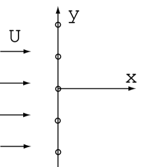
Figure 1: Kovasznay flow.

In the 2D stream-function formulation, when the velocity components are $u=\psi_{y}$ and $v=-\psi_{x}$, its dynamics obeys

$$\Delta\psi_{t}+\psi_{y}\Delta\psi_{x}-\psi_{x}\Delta\psi_{y}=0,$$ (2)

which after decomposition, $\psi=\Psi+\psi^{\prime}$, into the basic state $\Psi(x,y)=y$ periodic for $x>0$ with period $1$, and into the perturbation $\psi^{\prime}$ produces the following linearized evolution equation for $\psi^{\prime}$:

$$\Delta\psi_{t}^{\prime}+\Psi_{y}\Delta\psi_{x}^{\prime}=0.$$ (3)

Performing the standard eigenvalue analysis of (3), $\psi^{\prime}(t,x,y)\rightarrow\phi(x,y)e^{\lambda t}$, where in view of the solution periodicity in $y$-direction

$$\phi(x,y)=\sum_{n=0}^{\infty}{\alpha_{n}(x)\cos{2\pi ny}+\beta_{n}(x)\sin{2\pi ny}},$$ (4)

we find that all the mode amplitudes $\alpha_{n}(x)$ and $\beta_{n}(x)$ are decoupled, since the operator $\mathcal{L}=\left(\lambda+\partial_{x}\right)\Delta$ acting on $\phi(x,y)$ is of even order in $\partial_{y}$. Hence,

$$\left|\begin{array}[]{cccc}\mathcal{L}_{0}&&&0\\ &\mathcal{L}_{1}&&\\ &&\mathcal{L}_{2}&\\ 0&&&\ddots\end{array}\right|\cdot\left|\begin{array}[]{c}\alpha_{0}\\ \alpha_{1}\\ \alpha_{2}\\ \vdots\end{array}\right|=\bm{0},$$ (13)

that is each “amplitude” $\alpha_{n}$ satisfies

$$(\lambda+\mathrm{d}_{x})(\mathrm{d}_{x}^{2}-4\pi^{2}n^{2})\alpha_{n}(x)=0,\,n\in\mathbb{Z}^{+}.$$ (14)

For example, for $n=0$ let us contrast the solution of this eigenvalue problem on infinite and semi-infinite domains:

• $x\in(-\infty,+\infty)$: assuming that $y(x)\in L_{2}$, by applying Fourier transform we get $\lambda=-ik$, $k\in\mathbb{R}$, i.e. marginal stability.

• $x\in[0,+\infty)$ and $|y(x)|<\infty$: clearly, instability is present since there is an eigenfunction $y\sim e^{-\mu x}$, $\mu\geq 0$ such that the eigenvalue $\lambda=\mu$, which clearly leads to instability.

Same type of analysis can be done in the viscous case as well.

This counter-intuitive difference in the stability results between the semi-infinite and infinite domains can be appreciated with the sketch in figure 2. Namely, if, for example, one restricts (eigen-) functions $f(x)$ to be bounded for all $x$ including infinities as motivated by the physics, then the space of functions defined on $x\in(-\infty,+\infty)$ is more restricted compared to the space of functions defined on $x\in[0,+\infty)$. Indeed, if one can construct a function $f_{+}$ bounded on $x\in[0,+\infty)$ which also satisfies the Orr-Sommerfeld (OS) equation (15a), then continuation of this function onto $x\in(-\infty,0]$ may lead to an unbounded function $f_{-}$, as dictated by the structure of the linear Orr-Sommerfeld operator and as illustrated in figure 2.

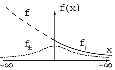
Figure 2: Semi- versus infinite flow domains. $f_{+}$ is defined on $x\in[0,+\infty)$, $f_{-}$ is defined on $x\in(-\infty,0]$, $f$ is defined on $x\in(-\infty,+\infty)$

Note that this explains the sensitivity of the critical bifurcation (Reynolds) number to the properties of disturbances at the domain inlet, $x=0$: while their amplitudes do not play a role in view of the linearity of the problem, gradient-like properties of the disturbances do! Indeed, varying these properties of disturbances at $x=0$, which may be masked by their amplitude, effectively changes the boundary conditions at $x=0$ and thus the size of the function space. Since restricting the domain to $x\in[0,+\infty)$ enlarges the function space, one can expect that the spectrum enlarges as well and may lead to instabilities.

Finally, just to reiterate on the crucial distinction of the stability on infinite versus semi-infinite domain, we remind the reader that an instability on a semi-infinite domain implies a growth of some eigenmode, say function $f_{+}$ defined only on a semi-infinite domain in figure 2. Then, if the domain is infinite, the unstable eigenmode $f_{+}$ obtained for a semi-infinite domain is not defined in general (cannot be continued for negative $x$ in the original function space, say the space of bounded function) and cannot grow in the part of the domain, where it is not defined.

II.2 Couette flow

One can expect that the analogous behavior should take place in the Couette and other “troublesome” flows. First recall that in the case of the Couette flow, Romanov Romanov rigorously proved that the disturbance defined on $x\in(-\infty,+\infty)$ and decaying at $x=\pm\infty$ can not lead to instability.

Let us show that the Couette flow is unstable on a semi-infinite domain as opposed to the case considered on an infinite domain. In the latter case, when the disturbance is defined on $-\infty<x<+\infty$ and decays at infinities, it is known Romanov that the upper bound of the real parts of the spectrum of the linear operator $A$ is $\sup\mathrm{Re}(\lambda)\leq-c/Re$ with $c>0$. If, on the other hand, analogously to the Kovasznay flow we consider the eigenfunctions $\phi(x,y)$ defined on $x\in[0,\infty)$, then assuming the separated form $\phi(x,y)=a(y)b(x)=a(y)e^{-\mu x}$ with $\mu\geq 0$ , we get the following eigenvalue problem for $a(y)$:

$$\lambda a_{yy}=Re^{-1}a_{yyyy},$$

$$y=-1,1:\,a=a_{y}=0,$$

which is given in the case $\mu=0$ (which according to the Fourier analysis should be present if the disturbance does not decay at $x=\infty$). The straightforward dispersion relation for this equation yields

$$\lambda=4\pi^{2}n^{2}\,Re^{-1},\,n\in\mathbb{N},$$

i.e. there is the eigenvalue $\lambda=0$ which gives marginal stability for any $Re$, as opposed to the result on the infinite domain.

While the above is the rigorous result on the stability of the Couette flow when the disturbances do not decay at infinity, one can apply heuristic Synge’s method to the general case, $\mu\geq 0$:

$$\left[{\mathrm{d}^{2}\over\mathrm{d}y^{2}}+\mu^{2}-Re\left(\lambda-\mu y\right)\right]\left({\mathrm{d}^{2}\over\mathrm{d}y^{2}}+\mu^{2}\right)a(y)=0,$$ (15a)

$$y=-1,1:\,a=a_{y}=0.$$ (15b)

Multiplying by $a^{*}$, integrating over $y\in[-1,1]$, and using the notation $I_{i}^{2}=\int_{-1}^{1}{|a^{(i)}|^{2}\,\mathrm{d}y}$, we get

$$Re\,\lambda(\mu^{2}I_{0}^{2}-I_{1}^{2})=I_{2}^{2}-2\mu^{2}I_{1}^{2}+\mu^{4}I_{0}^{2}$$

$$- Re\,\mu\left[\int_{0}^{1}{ya_{y}^{2}\,\mathrm{d}y}-\mu^{2}\int_{-1}^{1}{ya^{2}\,\mathrm{d}y}\right],$$

which in the limit $\mu\rightarrow+\infty$, physically corresponding to the localized disturbance at the inlet, yields

$$\lambda\sim Re^{-1}\mu^{2}>0,$$ (16)

i.e. one should observe an instability. The above asymptotics is, of course, valid only if the solution $a(y)$ does not have a strong dependence on $\mu$. While, as we will see shortly, $a(y)$ does depend on $\mu$, (16) turns out to give the right insight.

Rigorous dispersion relation for the Couette flow on semi-infinite domain can, in fact, be written down analytically. If we rewrite (15) in the operator form, $L_{1}L_{2}a(y)$, where $L_{1}={\mathrm{d}^{2}\over\mathrm{d}y^{2}}+\mu^{2}-Re\left(\lambda-\mu y\right)$ and $L_{2}={\mathrm{d}^{2}\over\mathrm{d}y^{2}}+\mu^{2}$, then we can exploit this factorization of the original forth-order operator in deriving the dispersion relation. First note that the kernel of these operators without boundary conditions are

$$\mathrm{ker}\,L_{1} =\mathrm{span}\left\{\mathrm{Ai}(\ldots),\mathrm{Bi}(\ldots)\right\},$$

$$\mathrm{ker}\,L_{2} =\mathrm{span}\left\{\sin(\ldots),\cos(\ldots)\right\}.$$

Thus, effectively we are solving

$$L_{2}^{00}a(y)=\alpha\mathrm{Ai}(\ldots)+\beta\mathrm{Bi}(\ldots),$$ (17)

where $L_{2}^{00}$ is the smaller operator with the boundary conditions (15b). Thus, in order to solve (17) one must have

$$\alpha\mathrm{Ai}(\ldots)+\beta\mathrm{Bi}(\ldots)\bot\mathrm{ker}\,L_{2}^{00*},$$

where $L_{2}^{00*}$ is the adjoint (not formally adjoint!) to $L_{2}^{00}$. Simple usage of the definition of adjoint

$$\langle v,L_{2}^{00}w\rangle=\langle L_{2}^{00*}v,w\rangle\equiv\langle L_{2}v,w\rangle$$ (18)

shows that $L_{2}^{00*}$ coincides with $L_{2}$, i.e. the operator without boundary conditions! Since we know the kernel of $L_{2}$, then for equation (17) and thus (15) to have a solution, it is necessary and sufficient that the Gram determinant vanishes:

$$\left|\begin{array}[]{cc}\left<\mathrm{Ai}|\cos\right>&\left<\mathrm{Ai}|\sin\right>\\ \left<\mathrm{Bi}|\cos\right>&\left<\mathrm{Bi}|\sin\right>\end{array}\right|=0.$$ (21)

In order to get some useful insights into the structure of a solution, let us analyze one of the entries of the above dispersion relation, e.g.

$$\left<\mathrm{Ai}|\cos\right>=\int_{-1}^{1}{\mathrm{Ai}(-\alpha y+\beta)\,\cos{\mu y}\,\mathrm{d}y},$$

where

$$\alpha=(\mu\mathrm{Re})^{1/3},\,\beta=\left({\lambda\over\mu}-{\mu\over Re}\right)\alpha.$$

As suggested by the asymptotics (16), it is tempting to consider the limit $\mu\gg 1$ and thus to exploit the stationary phase method, i.e. by considering $\cos{\mu y}$ as fast oscillating function and $\mathrm{Ai}(-\alpha y+\beta)$ as a slowly varying function. However, it turns out that for the given range of $y$ the periods of oscillation of both Airy and cosine functions are of the same order, which invalidates application of the stationary phase method. Another possible approach is to consider the Airy function with large arguments $|-\alpha y+\beta|\gg 1$, but then either $\lambda\sim O(1)$ leads to inconsistent asymptotics or $|\lambda|\gg 1$ invalidates the assumption of a uniform large argument $|-\alpha y+\beta|\gg 1$ for all $y$. In any case, large values of $\mu$ indeed turn out to produce interesting structure of the solution, as illustrated in figure 4 for $\mu$; higher values of $\mu$ increase the number of oscillations in the “accordion” structure.

In view of this fundamental difficulty to resolve this problem with the available rigorous analytical methods, we appealed to the numerical solution of (15) by expanding the solution into functions based on the complete set of the Chebyshev polynomials $T_{n}(y)=\cos{n\mathrm{arccos}\,y}$

$$a(y)=\sum_{i=0}^{N}{c_{i}\,\phi_{i}(y)},$$ (22)

which guarantee the convergence faster than any power of $N$ Orszag . Here the basis functions are given by

$$\phi_{i}(y)=T_{i}(y)-2{i+2\over i+3}T_{i+2}(y)+{i+1\over i+3}T_{i+4}(y),$$

i.e. they automatically satisfy the boundary conditions (15b). All the inner products associated with the Galerkin projection can be computed analytically, which is another advantage of this method.

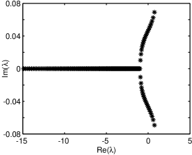
(a) Spectrum (eigenvalues continue to the negative part of the real axis.

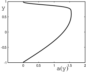
(b) Most unstable eigenfunction.

Figure 3: Spectral picture for the Couette flow at $Re=5000$ and $\mu=1$. The rightmost eigenvalue has real part $\mathrm{Re}\lambda_{\mathrm{max}}\simeq 0.75988755$ and the corresponding eigenfunction is shown in figure 3(b).

Since the goal here is not to study the complete bifurcation picture for the Couette flow, but to demonstrate that it is spectrally unstable for some finite Reynolds number, say $Re=5000$ and $\mu=1$. The resulting spectrum is shown in figure 3(a) and the eigenfunction corresponding to the eigenvalue with the largest real part in figure 3(b).

Figure 4: The eigenfunction corresponding to the rightmost eigenvalue has real part $\mathrm{Re}\,\lambda_{\mathrm{max}}\simeq 38.5314476$ for the Couette flow at $Re=5000$ and $\mu=40$.

As figure 3(a) clearly suggests, the transition in the Couette flow is of Hopf bifurcation type. For each fixed $\mu$ one can compute a critical Reynolds number $Re_{c}$, e.g. for $\mu=1$ we get $Re_{c}\simeq 75$. As $\mu$ increases, i.e. the disturbance is localized around the inlet, the value of $\mathrm{Re}\,\lambda_{\mathrm{max}}$ increases as well, as anticipated (16) and in agreement with the general observation at the end of §II.1. Note that there is nothing wrong with unbounded growth rates for infinite values of $\mu$, which is a common feature in many fundamental hydrodynamic instabilities in the short-wave limit, e.g. Rayleigh-Taylor instability. Of course, in the nonlinear setting one does not observe an infinite growth rates, which is suppressed by the nonlinear effects, which can also be dissipative as will be shown in §III. Also with increasing $\mu$ the eigenfunction structure becomes more complicated as we predicted in the above analytical study, e.g. for $Re=5000$ and $\mu=40$ the eigenfunction is shown in figure 4. More complete study of the stability picture for the Couette flow is out of the scope of this work and will be presented elsewhere.

III Nonlinear terms effects

As pointed out in the introduction, the usual argument made is that the linear terms in the NSEs are the only ones which produce energy and thus the nonlinear terms are energy-conserving and only mix energy between different modes Grossmann:II ; Henningson:II ; Henningson:I . The claim made in Henningson:II in the context of discussing shear flows with base state velocity field $\mathbf{U}$ is based on the consideration of the evolution of the kinetic energy $E(t)=\|\mathbf{u}\|^{2}/2$ of the disturbance velocity field $\mathbf{u}$ either over domains with periodic (i.e., compact domains) or homogeneous (zero) boundary conditions for disturbance, which leads to the classical Reynolds-Orr equation

$${\mathrm{d}E\over\mathrm{d}t}= -\nu\|\nabla\mathbf{u}\|^{2}-\left<D_{ij},u_{i}u_{j}\right>,$$ (23)

where $D_{ij}$ is the symmetric part of the base state velocity gradient tensor $\nabla\mathbf{U}$ . The linearity of (23), i.e. absence of the nonlinear terms effects, motivated the “transient-growth” idea of focusing only on the linear mechanisms.

The problem with the above argument is that the “troublesome” shear flows are defined not on either over domains with periodic (i.e., compact domains) or homogeneous (zero) boundary conditions for disturbance, but on domains with at least one semi- or unbounded dimension and the boundary condition of boundedness of the disturbance field at infinity. Thus, let us re-derive equation (23) taking into account that the boundary conditions on $\partial\Omega$ could be moved away to infinity. This leads to the following equation

$$-{\mathrm{d}E\over\mathrm{d}t}=\int\limits_{\partial\Omega}{n_{i}u_{i}p\,\mathrm{d}s}+\nu\int\limits_{\partial\Omega}{n_{j}u_{i}u_{i,j}\,\mathrm{d}s}+\nu\|\nabla\mathbf{u}\|^{2}$$ (24)

$$\left<D_{ij},u_{i}u_{j}\right>+\boxed{{1\over 2}\int_{\partial\Omega}{n_{j}u_{j}u_{i}u_{i}\,\mathrm{d}s}}+{1\over 2}\int_{\Omega}{n_{j}U_{j}u_{i}u_{i}\,\mathrm{d}x},$$

where $\mathbf{n}$ is the normal outward (w.r.t. $\partial\Omega$) vector and part or the whole of $\partial\Omega$ may be at infinity. If the domain $\Omega$ is unbounded, as in many applications, then the evaluation of the boundary terms in (24) becomes non-trivial, since it depends on the rate of the solutions decay in unbounded spatial directions , and therefore the nonlinear terms (cubic term in (24)) do not disappear, in general. In fact, there are no reasons to expect that these terms vanish in the Couette or other channel and pipe flows, since the disturbance, if it leads to an instability, does not decay as it propagates from the entrance to infinity. Moreover, if we consider the flow on a semi-infinite domain, as discussed in §II, then there is a non-zero contribution of the nonlinear terms at this portion of $\partial\Omega$ as well. As for open shear flows the nonlinear terms do not vanish since it is well-known that in order to construct a full set of eigenfunctions from the Orr-Sommerfeld equation, it is necessary to relax the homogeneous boundary conditions at infinity to the condition of boundedness at infinity, $|\mathbf{u}|_{|x|\rightarrow\infty}<\infty$, Salwen ; Grosch ; Herron:I , because the homogeneous boundary condition leads only to a finite set of a point discrete spectrum and therefore the inclusion of the continuous spectrum component is necessary for completeness. The completeness is of course important if one wants to study the question of stability rigorously. Therefore, one has to admit that the role of the nonlinear terms in the NSEs for shear flow problems is not a simple mixing of energy, but the disturbance energy can be denerated/dissipated by the nonlinearities.

Finally, another very important point is that the usual assertion that at early times the nonlinear effects are not important is not necessarily true since, for example, the linear term $\left<D_{ij},u_{i}u_{j}\right>$ and nonlinear one $-{1\over 2}\int_{\partial\Omega}{n_{j}u_{j}u_{i}u_{i}\,\mathrm{d}s}$ in equation (24) may become comparable even at small times either thanks to the very small values of $D_{ij}$ and/or the large cumulative effect of nonlinear terms when integrated over $\partial\Omega$ (possibly infinitely extended). In any case, no one has ever proved that this cannot occur for the flows in question!

It should be kept in mind that the energy is a nonlocal measure of the fluid motion, while in reality we are interested in the pointwise description, since we do not know much about the singular structure of the NSEs solution.

IV Other issues

For the purpose of the subsequent discussion discussion, it is convenient to treat the NSEs (1) as an infinite-dimensional ODE in the operator form in some Banach space $X$:

$${\mathrm{d}\mathbf{u}\over\mathrm{d}t}=A\mathbf{u}+N(\mathbf{u}),$$ (25)

where $A$ is the linear operator, usually stationary, and $N$ is the nonlinear operator. Historically, this approach allowed one to apply the dynamical systems methods of Dalekii & Krein Krein , Yudovich Yudovich:I for nonlinear stability of the equilibrium solutions of (25). Equation (25) can be obtained from (1) by utilizing the Helmholtz decomposition Chorin , i.e. through decomposing the solution vector field into the sum of its divergence- and curl-free components, e.g. $L^{p}(\Omega)=S^{p}(\Omega)\otimes G^{p}(\Omega)$, where $S^{p}(\Omega)$ is the Banach space obtained by closing the set of solenoidal vectors and $G^{p}(\Omega)$ is the Banach space obtained by closing the set of gradients in the norm of $L^{p}(\Omega)$. Then one can introduce the Leray projector $\mathbb{P}$, which projects any vector in $L^{p}(\Omega)$ onto $S^{p}(\Omega)$, and thus yields (25). In particular, if the stability of a nontrivial stationary (time-independent) base state $\mathbf{U}(\mathbf{x})$ is studied, then the linear and nonlinear operators in (25) take the form

$$A\mathbf{u} =\mathbb{P}\left[-\mathbf{U}\cdot\nabla\mathbf{u}-\mathbf{u}\cdot\nabla\mathbf{U}+Re^{-1}\Delta u\right],$$ (26a)

$$N(\mathbf{u}) =-\mathbb{P}\left[\nabla\cdot(\mathbf{u}\otimes\mathbf{u})\right].$$ (26b)

As follows from (26a), one can see the linear NSEs operator $A$ as a non-self-adjoint perturbation of the Laplace operator.

IV.1 Interrelation of stability notions

The notions of stability or instability, as physically observable phenomena, were given by Lyapunov Khalil . Namely, the equilibrium solution (base state) $\mathbf{u}^{e}\in X$ of (25) is said to be Lyapunov stable (sometimes called nonlinearly stable since (25) is nonlinear) if for any $\epsilon>0$ there exists a $\delta>0$ so that the initial conditions $\mathbf{u}_{0}\in X$ and $\|\mathbf{u}_{0}-\mathbf{u}^{e}(t_{0})\|_{X}<\delta$ imply that (i) there exists a solution $\mathbf{u}(t,t_{0},\mathbf{u}_{0})$ and (ii) $\|\mathbf{u}(t,t_{0},\mathbf{u}_{0})-\mathbf{u}^{e}(t)\|_{X}<\epsilon$ for all $t$. Then, the notion of Lyapunov instability is simply the negation of the above definition of stability. While this negation formally does not require existence to hold, i.e. the solution seizing to exist is a particular form of instability, from the physical point of view one does need existence in $X$ to get a sensible instability result Krechetnikov:II . Note that the linear stability is the Lyapunov stability of the linearized version of (25), $\mathbf{u}_{t}=A\mathbf{u}$ in the sense of the above definition. This should also be distinguished from the spectral stability, i.e. a formal notion obtained from the spectral problem, $A\mathbf{v}=\lambda\mathbf{v}$, associated with the linearized version of (25), when the spectrum is in the left half-plane.

There is a common view that linear eigenvalue analysis implies nonlinear Lyapunov stability, e.g. Henningson:I who, in the context of their discussion of the transition to turbulence, refer to Sattinger Sattinger in order to claim that a connection between linear and nonlinear stability has been established. However, in that work Sattinger demonstrated stability using the Reynolds-Orr equation, that is in a non-pointwise norm, for compact domains only, while the shear flows are usually considered on domains with at least one extended dimension. In general, as one can gather from most of the fluid dynamics literature, it is used as a rule: if the spectrum of the linearized operator (26a) is in the left half plane then one has stability and the instability takes place if there are eigenvalues in the right half plane. Below we first discuss the interrelation of all these notions in finite dimensions, and then address infinite dimensions in §IV.2.

Example 1.

First, consider a conservative system with the Hamiltonian $H(p,q)={p^{2}/2}+V(q)$, where the potential is quartic $V(q)=q^{4}/4$. As one can immediately see from the Hamilton’s equations, $q_{t}=p$ and $p_{t}=-q^{3}$, the linear and nonlinear stability of its equilibrium, $q=p=0$, definitions do not imply each other: this Hamiltonian system demonstrates nonlinear stability because the energy function is concave, but its linearization around the origin, $\dot{p}=0$ & $\dot{q}=p$, produces a solution growing linearly in time, i.e. it is linearly unstable. However, this example is spectrally stable; thus, spectral stability does not imply even linear stability, however the converse is true.

One might think that the above is a peculiar feature of the Hamiltonian dynamics, but in fact one observes the same for dissipative systems, e.g. for $q_{t}=p$ and $p_{t}=-q^{3}-p^{3}$.

Another example, discussed in Pollard (see also Siegel ) proves that linear stability does not imply nonlinear stability:

Example 2.

Given the Hamiltonian

$$H={1\over 2}(p_{1}^{2}+q_{1}^{2})-(p_{2}^{2}+q_{2}^{2})+{1\over 2}p_{2}(p_{1}^{2}-q_{1}^{2})-q_{1}q_{2}p_{1}.$$

from the corresponding Hamilton’s equations, we find that the origin, $\mathbf{q}=\mathbf{0}$ and $\mathbf{p}=\mathbf{0}$, is linearly stable, but a one-parameter, $\tau$, family of solutions for this system

$$p_{1} =\sqrt{2}\,{\sin(t-\tau)\over t-\tau}, \ p_{2} ={\sin{2(t-\tau)}\over t-\tau},$$

$$q_{1} =-\sqrt{2}\,{\cos{(t-\tau)\over t-\tau}}, \ q_{2} ={\cos{2(t-\tau)}\over t-\tau},$$

demonstrates nonlinear instability by blowing up at some finite time, $t=\tau$.

Therefore, from the above examples we conclude that

• linear instability does not imply nonlinear instability;

• linear stability does not imply nonlinear stability;

• spectral stability does not imply both linear and nonlinear stability,

However, spectral instability implies nonlinear instability in finite dimensions based on the classical Lyapunov indirect method Khalil .

IV.2 Infinite dimensionality effects

In infinite dimensions, the situation is even richer, because the latter property – the Lyapunov indirect method – does not hold in general. As mentioned in §IV.1, the usual approach is to base the conclusion of stability or instability of (25) on the spectrum $\sigma(A)$ of the linear operator $A$: if all eigenvalues lie strictly (i.e. no eigenvalues are on the imaginary axis) in the left half of the complex plane $\mathbb{C}$, then the zero solution is stable, while if there are eigenvalues in the left half-plane of $\mathbb{C}$, then the zero solution is unstable.

Let us discuss the question of linearized stability systematically . The solution of the linearized version of (25) which can be written symbolically as

$$\mathbf{u}(t)=\mathbf{u}(t_{0})\ e^{A(t-t_{0})}.$$ (27)

For a Banach space $X$ of finite dimension it is well known that if $\sup\limits_{\mathrm{Re}\,\lambda}{\lambda\in\sigma(A)}$ is $<0$, then $\|T(t)\|$ decays exponentially Pazy . This behavior is a consequence of the fact that linear operators in finite-dimensional Banach spaces have only point spectrum. Since this is not the case in infinite-dimensional Banach spaces one does not expect this result to be true in general. From a formal point of view, the exponent $e^{At}$ makes mathematical sense if the operator $A$ is bounded, i.e. $\|Ax\|_{X}\leq M\|x\|_{X}$ (in future we drop the index denoting the space $X$ in which the norm applies unless it becomes important to distinguish), so that

$$e^{At}=\sum\limits_{k=0}^{\infty}{A^{k}t^{k}/k!},$$ (28)

is well-defined, and from the spectral mapping theorem Engel one can connect the spectra $\sigma(A)$ and $\sigma(e^{At})$ via

$$\sigma(e^{At})=e^{t\sigma(A)}.$$ (29)

The convergence of (28) allows one to get a rough estimate, $\|e^{At}\|\leq\sum\limits_{k=0}^{\infty}{\|A\|^{k}t^{k}/k!}=e^{\|A\|t}$, $t>0$. However, the knowledge of the spectrum $\sigma(A)$ allows one to get sharper estimates: in particular, if $\|e^{A}\|\leq q$, the spectrum $\sigma(A)$ lies in the interior of $\mathrm{Re}\,\lambda\leq\log{q}$. If, however, the operator $A$ is unbounded, which is usually the case in hydrodynamics, then $e^{At}$ makes only symbolic sense and the equality is not true in general Phillips (see also Lax Lax:I , pp. 434–439) and, in fact, the spectral mapping property (29) does not hold, i.e.

$$\sigma(e^{At})\supset e^{t\sigma(A)},$$ (30)

from where it follows that one cannot conclude on stability of (25) based on the knowledge of spectrum of $\sigma(A)$. For unbounded operator the property (29) takes place only if it is an infinitesimal generator of an analytic semi-group, the convenient test for which is via proving that the operator is sectorial (cf. Henry Henry ), i.e. if its eigenvalues are contained in a cone sector with an apex angle $<\pi$ in the left-half of the complex plane.

These known facts can be most conveniently formulated with the help of two notions: spectral bound, $r(A)=\sup\left\{\mathrm{Re}\,\lambda|\,\lambda\in\sigma(A)\right\}$, and the growth abscissa of the semigroup, $\omega(A)=\lim\limits_{t\rightarrow\infty}{t^{-1}\log\left(\|e^{At}\|\right)}$. Then, in finite dimensions it is true that $\omega(A)=r(A)$, which is implicit in all studies of hydrodynamic stability. In the infinite-dimensional case, this equality is not true in general, as will be discussed below. However, some operators in certain spaces do possess this property, such as the Stokes operator is known Yudovich:I to generate an analytic semigroup in any $L^{p}$ space. Thus, one can expect that if (26a) is not a strong enough perturbation of the elliptic operator, which also depends on the boundary conditions, then the operator should still be a generator of an analytic semigroup.

On the other hand, there are many stability problems where the diffusive mechanisms, as controlled by elliptic operators (the Stokes, biharmonic, etc.), may be negligible, and thus $\omega(A)\neq r(A)$. For example, hyperbolic PDEs exhibit such behavior, as can be illustrated with the following simple example due to Renardy Renardy:I

Example 3.

Consider the following hyperbolic equation:

$$u_{tt}=u_{xx}+u_{yy}+e^{iy}u_{x},$$ (31)

with $2\pi$-periodic boundary conditions in both directions. Introducing $v=u_{t}$, the semigroup operator $A$ associated with (31) is $A(u,v)=\left(v,u_{xx}+u_{yy}+e^{iy}u_{x}\right)$, which in fact generates a $C_{0}$-semigroup in the space $H^{1}\times L^{2}$ for the pair $(u,u_{t})$. The analysis Renardy:I demonstrates that $r(A)=0$, while $\omega(A)=1/2$.

In general, it is well-known after the work of Zabczyk Zabczyk that for any two real numbers $\omega_{s}<\omega_{0}$ there exists a strongly continuous semigroup $\{T_{t}\}_{t\geq 0}$ on a Hilbert space, such that $\omega_{s}=\sup\left\{\mathrm{Re}\,\lambda;\,\lambda\in\sigma(A)\right\}$ and $\left|T_{t}\right|=e^{\omega_{0}t},\ t\geq 0$, where $\sigma(A)$ denotes the spectrum of the generator $A$ of the semigroup $\{T_{t}\}_{t\geq 0}$.

The above most systematically can be understood in terms of classification of semi-groups Pazy , namely parabolic versus hyperbolic, as resulted from the application of the abstract semi-group theory to evolution partial differential equations. In the parabolic case the operators are the infinitesimal generators of an analytic semi-group, while in the hyperbolic case one can expect the behavior as in the above example 3 due to Renardy Renardy:I . While behavior of example 3 is common for Hamiltonian systems, in which the eigenvalues are distributed symmetrically w.r.t both axes in the complex plane and the placement of all eigenvalues on the imaginary axis is a necessary but not a sufficient condition for stability of an equilibrium, equation (31) is clearly non-conservative, which suggests that such pathologies in the linear stability picture are common for dissipative systems too.

First of all, the existence and (in)stability of the solutions of the full nonlinear system (25) are most conveniently (at the current level of mathematics) studied by transforming it into the integral form via Duhamel’s formula

$$\mathbf{u}(t)=\mathcal{T}(\mathbf{u})=\mathbf{u}(0)e^{At}+\int\limits_{0}^{t}{e^{A(t-\tau)}\,N(\mathbf{u}(\tau))\,\mathrm{d}\tau},$$ (32)

which is not only used to solve (25) using fixed point theorems for the mapping $\mathcal{T}(\mathbf{u})$, but also clearly illustrates the importance of both the linear terms – the semigroup $\{e^{At}\}_{t\geq 0}$ – and the nonlinear terms in infinite dimensions. Indeed, on any relevant to this discussion Banach space $X$ the nonlinear terms will be unbounded in view of the presence of unbounded operator of differentiation in (26b), which can be compensated only by the smoothing effect of the semigroup $e^{A(t-\tau)}$. The latter can happen, of course, only if the semigroup is “nice” enough. This illustrates the importance of consideration of both linear and nonlinear effects when studying the questions of stability. Formula (32) is the basis of all rigorous stability studies, such as due to Krein Krein , Henry Henry , and Yudovich Yudovich:I .

Thus, it is not surprising that infinite dimensionality may lead to pathologies, which are not possible in finite dimensions. For example, in the context of elasticity problems it is known that the positive definite second variation of the energy (and thus the corresponding system should be nonlinearly stable according to the Dirichlet theorem, valid in finite dimensions only) does not guarantee the stability in view of the possible presence of an infinite number of unstable directions Ball:I .

Another complication arising due to infinite dimensionality is the norm-dependence of stability criteria – the issue which has been understood for a long time Yudovich:I ; Friedlander:II . In the finite-dimensional case this difficulty cannot arise since all norms in finite-dimensional Banach spaces are equivalent.

Example 4.

One of the simplest examples of this subtlety is due to Yudovich:I and represents a linear PDE:

$${\partial u\over\partial t}=x{\partial u\over\partial x},$$

$$u(0,x)=\phi(x),$$

the unique solution of which is $u(x,t)=\phi\left(x\ e^{t}\right)$. Thus one can express the $L^{p}$-norm of the solution derivatives via $\left\|{\partial^{k}u(\cdot,t)\over\partial x^{k}}\right\|_{L^{p}(\mathbb{R})}=e^{(k-p^{-1})t}\left\|\phi^{(k)}\right\|_{L^{p}(\mathbb{R})}$, and therefore one has (a) asymptotic stability in $L^{p}(\mathbb{R})$ for $1\leq p<\infty$, (b) Lyapunov stability in $L^{\infty}(\mathbb{R})$, and (c) exponential instability in Sobolev spaces $W^{k,p}(\mathbb{R})$ with $k>1$, $p\geq 1$ or $k=1$, $p>1$.

Finally, quite often by “nonlinear stability” one understands “energy stability”, which is not quite correct, since nonlinear stability is a stability in the Lyapunov pointwise sense, while the energy norm is a global measure . In order to make a pointwise sense of the energy-like norms, so that the function belongs to the Hölder space of $k$-times continuously differentiable functions $f\in C^{k}$, one needs energy-like bounds for the solution derivatives, that is $f$ should belong to the Hilbert space $H^{k}$ with high enough index, so that one can employ the Sobolev inequality; e.g. in the two-space dimensions:

$$\left|f\right|_{C^{k}}\leq C\|f\|_{H^{k+s}},\ s\geq 1.$$

From here it follows that establishing bounds on the usual kinetic energy norm $H^{0}$ is not enough to assert the bounds on the solution, and thus to claim the stability of the solutions in the Lyapunov sense.

IV.3 Non-normality and covariance

Starting with Trefethen et al. Trefethen:I the following two-dimensional model is very popular Henningson:I for illustrating what is “supposed” to happen in the transition problem

$${\mathrm{d}\mathbf{u}\over\mathrm{d}t}=A\mathbf{u}+\mathbf{F}(\mathbf{u}),\ A=\left(\begin{array}[]{cc}-a_{1}&1\\ 0&-a_{2}\end{array}\right),$$ (35)

where $A$ is a non-normal operator in a sense that $A\,A^{*}\neq A^{*}\,A$, where $A^{*}$ is the adjoint operator, with $a_{1,2}\sim Re^{-1}$ being small exponents determining the time-evolution, and $\mathbf{F}(\mathbf{u})$ is a nonlinear energy conserving operator and. Since the linear operator $A$ is non-normal, then its eigenvectors corresponding to the eigenvalues $\lambda_{1}=-a_{1}$ and $\lambda_{2}=-a_{2}$ are almost parallel for $Re\gg 1$, which in the case used by Trefethen et al. Trefethen:I , $a_{1}=Re^{-1}$ and $a_{2}=2\,Re^{-1}$, are:

$$\mathbf{e}_{1}=\left[\begin{array}[]{c}1\\ 0\end{array}\right],\ \mathbf{e}_{2}=\left[\begin{array}[]{c}1\\ -Re^{-1}\end{array}\right].$$ (40)

In the limit $Re\rightarrow\infty$ the matrix $A$ becomes the non-trivial Jordan block, when the solution $\mathbf{u}$ grows algebraically. Due to this non-normality for finite $Re$, the system $\dot{\mathbf{u}}=A\mathbf{u}$ experiences a transient growth for $t=O(Re)$, e.g. for the initial conditions $\mathbf{u}(0)=\left[0,1\right]^{T}$:

$$\mathbf{u}(t) =\left[\begin{array}[]{c}Re\\ 0\end{array}\right]e^{-{t\over Re}}+\left[\begin{array}[]{c}-Re\\ 1\end{array}\right]e^{-{2t\over Re}}$$ (45)

$$=\left[\begin{array}[]{c}t+O\left(t^{2}\over Re\right)\\ 1-{2t\over Re}+O\left(t^{2}\over Re^{2}\right)\end{array}\right].$$ (48)

Next, the key dynamic feature of all these models is the presence of a finite-amplitude instability; in the case of Trefethen et al. Trefethen:I the nonlinearity is $\|\mathbf{u}\|B\mathbf{u}$ with $B=\left(\begin{array}[]{cc}0&-1\\ 1&0\end{array}\right)$, which has three stable nodes (one at the origin) and two saddle points, while Manneville Manneville:I used $\mathbf{F}(\mathbf{u})=\left(uv,-u^{2}\right)^{T}$, which has two stable nodes (one is at the origin) and a saddle. Manneville used example (35) to advocate that the non-normality of the linear operator is not in itself responsible for the by-pass transition, while Trefethen et al. Trefethen:I insisted that the transition is “essentially linear”. While the form of Trefethen’s nonlinearity was criticized Waleffe:I as not relevant to the NSEs, it is clear that it cannot be obtained as a result of some kind of reduction from the NSEs, since the square root is not Taylor expansion-friendly.

If one expects that transition is a fundamental physical phenomenon, then it must be accounted in a covariant (coordinate-free) manner, that is its understanding should be independent of the coordinate system. Thus, let see if model (35) possesses this property.

In this subsection we consider the linear part of (35) recalling some elementary facts, while in the next section we discuss the fully nonlinear dynamics. Even though the original matrix $A$ in (35) is non-normal, there exists a transformation which makes this linear operator in (35) normal. Clearly, normal matrices are a subset of the diagonizable matrices and the relation between normal and diagonizable matrices is well-understood Mitchell . The notion of diagonizability is an intrinsic notion (that is, independent of a coordinate system) as opposed to to non-normality, since the latter notion depends upon a system of coordinates. In terms of genericity notion, cf. Wiggins Wiggins , i.e., informally, how common are the physical systems with non-normal operators, it is obvious that non-normal matrices form a dense subset in the set $C^{n^{2}}$ of all $n\times n$ matrices. Further, we will comment on the infinite-dimensional operators, but first consider the finite dimensional case as relevant to the discussion of model (35). In fact, this clear understanding of which notions are intrinsic or not shades some light on the claims that the non-normal linear operators is the key to transition. Appealing to the standard matrix theory Franklin , let us consider a linear transformation $A$ on the Euclidean space $\mathbb{E}^{n}$, which maps the vector $\mathbf{x}$ into $\mathbf{x}^{\prime}$: $\mathbf{x}^{\prime}=A\mathbf{x}$. If matrix $T$ consists of the basis vectors $\mathbf{t}^{1},\ldots,\mathbf{t}^{n}$, then $\mathbf{x}=T\mathbf{y}$ and $\mathbf{x}^{\prime}=T\mathbf{y}^{\prime}$, where $\mathbf{y}$ and $\mathbf{y}^{\prime}$ are components of the corresponding vectors $\mathbf{x}$ and $\mathbf{x}^{\prime}$. Note that $\mathrm{det}\,T\neq 0$ since it forms a basis. Then, the relation between $\mathbf{y}$ and $\mathbf{y}^{\prime}$ is simply $\mathbf{y}^{\prime}=T^{-1}\,A\,T\,\mathbf{y}$. Matrices $A$ and $T^{-1}\,A\,T$ are similar, and $T^{-1}\,A\,T$ can be made diagonal (and thus normal) if and only if $A$ has $n$ linearly independent eigenvectors (in particular, if $A$ has distinct eigenvalues, but not necessarily). Of course, if the matrix $A$ is originally normal, then it will have orthogonal eigenvectors and thus $T$ will be orthogonal, which means that normality will be ‘preserved’. Anyway, non-normal matrices may be reduced to normal ones under appropriate change of coordinates. Since we looking for a covariant description of physical phenomena, i.e. independence of our understanding of the phenomena of a coordinate system, then it becomes clear that non-normality has nothing to do with the covariant understanding of the fundamental cause of the transition. While the transient growth effects may be important exactly as “transient” effects, which can be most clearly seen through the singular value decomposition, on the time scales greater than the transient growth time, e.g. $t>Re^{-1}$ in (48), their effect is not relevant in any coordinate system. Becides these general remarks, one should also point out from the positions of control theory that not all non-normal operators can lead to significant transient effects, but only those which possess some high sensitivity subspaces in their domain of definition together with the presence of disturbances in this subspace.

The above discussion for operators in finite-dimensional spaces can be translated to the case of infinite-dimensional operators, as we discuss here in the context of PDEs. Clearly, the linear operator in the NSEs (26a) is non-normal for non-trivial base states $\mathbf{U}(\mathbf{x})$. The degree of non-normality of (26a) increases as the Reynolds number increases since the self-adjoint part of (26a) , that is the Laplacian, becomes less dominant. Most clearly, this probably can be seen in a spectral space after the Galerkin projection. In any case, the non-normality of the partial differential operator leads to a transient in time growth in the same way as a non-normal matrix-operator, which is a self-evident fact, but nevertheless quite a number of works were devoted to illustrate this behavior in the context of the NSEs Reddy ; Bamieh .

IV.4 Finite-amplitude effects

From the nonlinear covariant analysis viewpoint, it is tempting to perform the normal form analysis of (35) in order to reveal the universal behavior of (35). However, the local nature of the normal form analysis, i.e. inability to get the global bifurcation picture, does not allow one to capture the finite-amplitude instabilities inherent in (35): e.g. in the non-resonant case of $a_{1}$ and $a_{2}$ in (35), the normal form is simply

$${\mathrm{d}\mathbf{x}\over\mathrm{d}t}=J\mathbf{x},\ J=\left(\begin{array}[]{cc}-a_{1}&0\\ 0&-a_{2}\end{array}\right),$$ (51)

and in the resonant case, $a_{2}=2a_{1}$ is

$${\mathrm{d}\mathbf{x}\over\mathrm{d}t}=J\mathbf{x}+\left(\begin{array}[]{c}0\\ ax_{1}^{2}\end{array}\right),\,a\in\mathbb{R}.$$ (54)

Both the above normal forms do not exhibit finite-amplitude instabilities. This fundamental inability of the normal form analysis to capture the global bifurcation picture can be understood with the following simple example, which also leads to some further insights.

Example 5.

Let us consider the following equation

$${\mathrm{d}x\over\mathrm{d}t}=-\epsilon x+x^{2},$$ (55)

which describes transcritical bifurcation and exhibits a finite-amplitude instability with the critical amplitude $x_{c}=\epsilon$. With the goal to reduce this equation to a linear equation

$${\mathrm{d}y\over\mathrm{d}t}=-\epsilon y,$$ (56)

let us introduce a transformation, $x=y+F(y)$, where $F(y)$ is a function to be determined. Substitution of this transformation into (55) gives

$${\mathrm{d}y\over\mathrm{d}t}[1+F^{\prime}(y)]=-\epsilon[y+F(y)]+[y+F(y)]^{2}.$$ (57)

In the standard treatment of the local normal form analysis (e.g. Wiggins ), one assumes that $|F^{\prime}(y)|\ll 1$ and thus inverts $[1+F^{\prime}(y)]$ approximately, i.e. $[1+F^{\prime}(y)]^{-1}\simeq 1-F^{\prime}(y)$. In fact, one does not need this approximate procedure in order to get an equation for $F(y)$: instead, one multiplies (56) by $F^{\prime}(y)$ and subtracts from (57):

$${\mathrm{d}y\over\mathrm{d}t}=-\epsilon y-\epsilon F(y)+\epsilon yF^{\prime}(y)+[y+F(y)]^{2},$$ (58)

that is, $F(y)$ is determined from

$$\epsilon[F-yF^{\prime}]=[y+F]^{2},$$ (59)

with the result

$$F(y)={\epsilon y\over y-\alpha}-y,$$ (60)

where $\alpha\neq 0$ for the transformation $x=y+F(y)$ to be non-singular. Thus, for $x\neq\epsilon$ the transformation $x=y+F(y)$ “straightens out” the trajectories of the original system (55) and produces a trivial dynamics as in (56), but is singular for $x=\epsilon$.

The latter property, i.e. singularity of the transformation which linearizes the dynamics globally except for at the threshold amplitudes can be used to identify the presence and location of the finite-amplitude instabilities in the appropriate configuration (phase) spaces.

The indicated in the introduction possibility of finite-amplitude instability nature of the transition suggested a search for finite-amplitude solutions in the shear flows. For example, Nagata Nagata:I found a finite-magnitude periodic solutions in the Couette flow, which coexists with the linear Couette profile, appealing to the concept bifurcation from infinity Rosenblat . The travelling wave-like solutions are known both in the context of the pipe Faisst and plane Couette Nagata:II flows. However, their “strongly unstable character”, since they are all saddle points in phase space Kerswell:I , is also well-known Eckhardt . The latter work also advocates that the turbulent state in pipe flow corresponds to a chaotic saddle (unstable aperiodic orbit) in state space. The idea is that travelling wave solutions presumably constitute a ‘skeleton’ about which complicated time-dependent orbits may drape themselves temporarily before falling back to the laminar state Kerswell:I .

Waleffe Waleffe:I advocated the idea of exploring the size of the domain of attraction of the finite-amplitude solutions following the original thoughts of Orr and Thomson. Also, Trefethen et al. Trefethen:I conjectured that the non-normality of the linear operator shrinks the size of the attraction basin and, in fact, the threshold amplitude scales as $Re^{-\gamma}$.

The above dynamical systems approach is based on the finite-dimensional view of the NSEs dynamics. The latter is usually justified Kerswell:I by the argument that the motion of a viscous fluid in a finite domain is always finite-dimensional which is due to the viscous cutoff of fine scales with reference to Constantin . However, the troublesome flows always have at least one unbounded dimension, which undermines the above logic and poses the question on the possible crucial effect of infinite-dimensionality. Next, as currently understood, all these finite-amplitude solutions proved to be unstable. Moreover, it is very likely that if the transition is indeed a finite-amplitude instability, the attracting solutions in fact are intrinsically time-dependent or even chaotic and occupy some subset of the phase space. Thus, there is little hope to find the corresponding solutions analytically.

V Discussion

The purpose of this note was to bring a number of important theoretical issues to the attention of the fluids community, solving of which may help to make some progress on a reasonable qualitative understanding and quantitative prediction of the experimental observations, which are still lacking. In particular, as follows from §II and §III, exploring the effects of the domain type and of the energy conservation by nonlinear terms are the first natural issues to address systematically.

The authors also see two other possible ways of exploring the problem of transition rigorously. The first way is to develop a semi-local nonlinear stability theory, which could be a natural generalization of the stability theory due to Krein, Yudovich, and Henry by inclusion of the finite-amplitude instability picture in consideration. The second possible avenue is to gain insights into the geometric structure of the equations, which allow one to identify the possible regions of attraction in the phase space and thus to establish the stability picture in large (i.e. both local, global, finite-amplitude, etc.). Namely, one first explores the phase space structure of the Hamiltonian approximation (ideal fluid) and, if this is not sufficient for explaining the instability picture, one adds dissipative effects (viscosity). In particular, this would allow one to understand if the fundamental basis of the transition phenomena is Hamiltonian or intrinsically due to dissipative (viscous) effects; see also Krechetnikov:II . The reader can easily appreciate the effectiveness of this approach with the help of, say, the Takens-Bogdanov system Lewis :

$$\ddot{x}=\mu-x^{2}=-V_{x},\ V(x)=-\mu x+{x^{3}/3}.$$ (61)

Namely, locating maxima and minima of the potential $V(x)$ (or alternatively of the Hamiltonian) indicates the stability picture. This idea, of course, is very old and goes back to Lagrange, Dirichlet and other classics. Next, one adds dissipative effects Krechetnikov and observes how the stability picture changes. The infinite-dimensional case is, of course, more complicated, but some progress has been done in this direction as well Krechetnikov:II .

Finally, while all the previous fluid mechanics experience over the last few centuries suggests that the NSEs are the adequate description of fluid motion, strictly speaking one cannot discard the chance that the NSEs do not describe the subtle transition to turbulence phenomena. One can name many reasons for which the NSEs may turn out to be inappropriate for modeling of the transition. For example, since the transition is a phenomenon presumably very sensitive to initial and boundary conditions, then it should be very sensitive to the details of the equations. Since Newtonian fluid description is an approximate one, then in the conventional NSEs for incompressible fluid we discard by hyperbolic effects common for non-Newtonian fluids. Same can be said about the incompressibility approximation. While one might argue that these effects may have an influence only at some marginal time and spatial scales, the history of hydrodynamics knows a number of fundamental examples when small effects affect the flow in the large (Prandtl’s boundary layer theory, for instance).

VI Acknowledgements

R.K. would like to thank the attendees of the session on transition in shear flows at the Second Canada-France Congress (June 1-6, 2008), where the presented here results were announced, for the feedback.

References

- (1) P.G. Drazin and W.H. Reid. Hydrodynamic stability. Cambridge University Press, 1984.
- (2) T. Mullin and J. Peixinho. Transition to turbulence in pipe flow. J. Low Temp. Phys., 145:75–88, 2006.
- (3) L. N. Trefethen, A. E. Trefethen, S. C. Reddy, and T. A. Driscoll. Hydrodynamic stability without eigenvalues. Science, 261:578–584, 1993.
- (4) D. S. Henningson and S. C. Reddy. On the role of linear mechanisms in transition to turbulence. Phys. Fluids, 6:1396–1398, 1994.
- (5) S. C. Reddy and D. S. Henningson. Energy growth in viscous channel flows. J. Fluid Mech., 252:209–238, 1993.
- (6) V. A. Romanov. Stability of plane-parallel Couette flow. Functional Anal. & its Applications, 7:137–146, 1973.
- (7) D. Gottlieb and S. A. Orszag. Numerical Analysis of Spectral Methods: Theory and Applications. SIAM, Philadelphia, Pennsylvania, 1977.
- (8) S. Grossmann. Instability without instability?, pages 10–22. Springer, 1996.
- (9) D. Henningson. Comment on “Transition in shear flows. Nonlinear normality versus non-normal linearity”. Phys. Fluids, 8:2257–2258, 1996.
- (10) H. Salwen and C. E. Grosch. The continuous spectrum of the Orr-Sommerfeld equation. Part 1. Eigenfunction expansions. J. Fluid Mech., 104:445–465, 1981.
- (11) C. E. Grosch and H. Salwen. The continuous spectrum of the Orr-Sommerfeld equation. Part 2. The spectrum and the eigenfunctions. J. Fluid Mech., 87:33–54, 1978.
- (12) I. H. Herron. The Orr-Sommerfeld equation on infinite intervals. SIAM Rev., 29:597–620, 1987.
- (13) Ju. L. Daleckii and M. G. Krein. Stability of solutions of differential equations in Banach space. AMS, Providence, 1974.
- (14) V. I. Yudovich. The linearization method in hydrodynamical stability theory. AMS, Providence, 1989.
- (15) A. J. Chorin and J. E. Marsden. A Mathematical Introduction to Fluid Mechanics. Springer, 1993.
- (16) H. K. Khalil. Nonlinear systems. Prentice Hall, 2002.
- (17) R. Krechetnikov and J. E. Marsden. Dissipation-induced instability phenomena in infinite-dimensional systems. 2008. to appear in Arch. Rat. Mech. Anal.
- (18) D. H. Sattinger. The mathematical problem of hydrodynamic stability. J. Math. Mech., 19:797–817, 1970.
- (19) H. Pollard. Mathematical introduction to celestial mechanics. Prentice-Hall, Englewood Cliffs, 1966.
- (20) C. L. Siegel and J. K. Moser. Lectures on celestial mechanics. Springer-Verlag, New York, 1971.
- (21) A. Pazy. Semigroups of linear operators and applications to partial differential equations. Springer-Verlag, New York, 1983.
- (22) K.-J. Engel and R. Nagel. One-Parameter Semigroups for Linear Evolution Equations. Springer, 1999.
- (23) R. S. Phillips. Spectral theory of semigroups of linear operators. Trans. AMS, 74:393–415, 1951.
- (24) P. D. Lax. Functional Analysis. Wiley-Interscience, 2002.
- (25) D. Henry. Geometric theory of semilinear parabolic equations. Springer-Verlag, New York, 1981.
- (26) M. Renardy. On the linear stability of hyperbolic pdes and viscoelastic flows. Z. Angew. Math. Phys., 45:854–865, 1994.
- (27) J. Zabczyk. A note on semigroups. Bull. Acad. Polon. Sci., 23:895–898, 1975.
- (28) J. M. Ball and J. E. Marsden. Quasiconvexity, second variations and nonlinear stability in elasticity. Arch. Rat. Mech. An., 86:251–277, 1984.
- (29) S. Friedlander and V. Yudovich. Instabilities in fluid motion. Notices of Amer. Math. Soc., 46:1358–1367, 1999.
- (30) P. Manneville. Modeling the direct transition to turbulence. Fluid Mech. Appl., 77:1–34, 2005.
- (31) F. Waleffe. Transition in shear flows. Nonlinear normality versus non-normal linearity. Phys. Fluids, 7:3060–3066, 1995.
- (32) B. E. Mitchell. Normal and diagonalizable matrices. The American Mathematical Monthly, 60:94–96, 1953.
- (33) S. Wiggins. Introduction to Applied Nonlinear Dynamical Systems and Chaos. Springer, 2003.
- (34) J. N. Franklin. Matrix theory. Prentice Hall, 1968.
- (35) B. Bamieh and M. Dahleh. Energy amplification in channel flows with stochastic excitation. Phys. Fluids, 13:3258–3269, 2001.
- (36) M. Nagata. Three-dimensional finite-amplitude solutions in plane Couette flow: bifurcation from infinity. J. Fluid Mech., 217:519–527, 1990.
- (37) S. Rosenblat and S. H. Davis. Bifurcation from infinity. SIAM J. Appl. Math., 37:1–19, 1979.
- (38) H. Faisst and B. Eckhardt. Traveling waves in pipe flow. Phys. Rev. Lett., 91:224502, 2003.
- (39) M. Nagata. Three-dimensional traveling-wave solutions in plane Couette flow. Phys. Rev. E, 55:2023–2025, 1997.
- (40) R. R. Kerswell. Recent progress in understanding the transition to turbulence in a pipe. Nonlinearity, 18:17–44, 2005.
- (41) B. Eckhardt, T. M. Schneider, B. Hof, and J. Westerweel. Turbulence transition in pipe flow. Annu. Rev. Fluid Mech., 39, 2007.
- (42) P. Constantin, C. Foias, O. P. Manley, and R. Temam. Determining modes and fractal dimension of turbulent flows. J. Fluid Mech., 150:427–440, 1985.
- (43) D. Lewis and J. Marsden. A Hamiltonian-dissipative decomposition of normal forms of vector fields. In in the Proceedings of the International conference on ”Bifurcation theory and its numerical analysis”, pages 51–78, China, 1988.
- (44) R. Krechetnikov and J. E. Marsden. Dissipation-induced instabilities in finite dimensions. Rev. Mod. Phys., 79:519–553, 2007.
- (45) B. Straughan. The energy method, stability, and nonlinear convection. Springer, 1991.
- (46) V. I. Arnold. On matrices depending on parameters. Russ. Math. Surv., 26:29–43, 1971.