X-ray spectra from magnetar candidates. II. Resonant cross sections for electron-photon scattering in the relativistic regime

Abstract

Recent models of spectral formation in magnetars called renewed attention on electron-photon scattering in the presence of ultra-strong magnetic fields. Investigations presented so far mainly focussed on mildly relativistic particles and magnetic scattering was treated in the non-relativistic (Thomson) limit. This allows for consistent spectral calculations up to a few tens of keVs, but becomes inadequate in modelling the hard tails ($\la 200$ keV) detected by INTEGRAL from magnetar sources. In this paper, the second in a series devoted to model the X-/soft $\gamma$-ray persistent spectrum of magnetar candidates, we present explicit, relatively simple expressions for the magnetic Compton cross-section at resonance which account for Landau-Raman scattering up to the second Landau level. No assumption is made on the magnetic field strength. We find that sensible departures from the Thomson regime can be already present at $B\sim 5\times 10^{12}$ G. The form of the magnetic cross section we derived can be easily implemented in Monte Carlo transfer codes and a direct application to magnetar spectral calculations will be presented in a forthcoming study.

1 Introduction

The recent discovery with the INTEGRAL satellite of hard X-ray tails in the (persistent) spectra of the magnetar candidates (the anomalous X-ray pulsars, AXPs, and the soft $\gamma$-repeaters, SGRs; e.g. Mereghetti 2008) provides evidence that a sizeable fraction (up to $\sim 50\%$) of the energy output of these sources is emitted above $\sim 20$ keV. Up to now, high-energy emission has been detected in two SGRs, 1806-20 and 1900+14 (Mereghetti et al., 2005; Götz et al., 2006), and three AXPs, 4U 0142+614, 1RXS J170849-4009 and 1E 1841-045 (Kuiper, Hermsen & Mendez, 2004; Kuiper et al., 2006, see also for an updated summary of INTEGRAL observations Götz 2008) . This result come somehow unexpected, since the spectra of SGRs/AXPs in the soft X-ray range ($\sim 0.1$–10 keV) are well described by a two component model, a blackbody at $kT\sim 0.2$–0.6 keV, and a rather steep power-law with photon index $\Gamma_{soft}\sim 1.5$–4. INTEGRAL observations have shown that in SGRs the power-law tail extends unbroken (or steepens) in the $\sim 20$–200 keV range, $\Gamma_{hard}\ga\Gamma_{soft}\sim 1.5$. In AXPs, which have steeper spectra in the soft X-ray band, a spectral upturn appears, i.e. the high-energy power-law is harder than the soft one, $\Gamma_{hard}\sim 1$ while $\Gamma_{soft}\sim 3$–4 (see e.g. Rea et al., 2008, for a joint spectral analysis of XMM-Newton and INTEGRAL data).

Within the magnetar scenario, the persistent 0.1–10 keV emission of SGRs and AXPs has been successfully interpreted in terms of the twisted magnetosphere model (Thompson, Lyutikov & Kulkarni, 2002). In an ultra-magnetized neutron star the huge toroidal field stored in the interior produces a deformation of the crust. The displacement of the footprints of the external (initially dipolar) field drives the growth of a toroidal component which, in turn, requires supporting currents. Charges flowing in the magnetosphere provide a large optical depth to resonant cyclotron scattering (RCS) and repeated scatterings of thermal photons emitted by the star surface may then lead to the formation of a power-law tail. The original picture by Thompson, Lyutikov & Kulkarni (2002) has been further explored by Lyutikov & Gavriil (2006), Fernandez & Thompson (2007) and Nobili, Turolla & Zane (2008, hereafter paper I). Recently Rea et al. (2008) presented a systematic application of the 1D, analytical RCS model of Lyutikov & Gavriil (2006) to a large sample of magnetars X-ray spectra finding a good agreement with data in the 0.1–10 keV range. As shown in paper I, more sophisticated 3D Monte Carlo calculations of RCS spectra successfully reproduce soft X-ray observations.

Despite the twisted magnetosphere scenario appears quite promising in explaining the magnetars soft X-ray emission, if and how it can account also for the hard tails detected with INTEGRAL has not been unambiguously shown as yet. Thompson & Belobodorov (2005) suggested that the hard X-rays may be produced either by thermal bremsstrahlung in the surface layers heated by returning currents, or by synchrotron emission from pairs created higher up ($\approx 100$ km) in the magnetosphere. Baring & Harding (2007, 2008) have recently proposed a further possibility, according to which the soft $\gamma$-rays may originate from resonant up-scattering of seed photons on a population of highly relativistic electrons. Previous investigations (Lyutikov & Gavriil 2006; Fernandez & Thompson 2007; paper I) mainly focussed on mildly relativistic particles and magnetic scattering was treated in the non-relativistic (Thomson) limit. This is perfectly adequate in assessing the spectral properties up to energies $\ll m_{e}c^{2}/\gamma$ (here $\gamma$ is the typical electron Lorentz factor) since i) the energy of primary photons is low enough ($\approx 1$ keV) to make resonant scattering onto electrons possible only where the magnetic field has dropped well below the QED critical field, ii) up-scattering onto electrons with $\gamma\approx 1$ hardly boosts the photon energy in the hundred keV range, so electron recoil is not important. However, some photons do actually gain quite a large energy (because they scatter many times on the most energetic electrons) and fill a tail at energies $\ga 50$ keV. We caveat that, despite in previous works spectra have been computed up to the MeV range, they become untrustworthy above some tens of keV and can not be used to assess the spectral features that can arise due to electron recoil effects (i.e. a high-energy spectral break). Proper investigation of the latter demands a complete QED treatment of magnetic Compton scattering. This is mandatory if highly relativistic particles are considered because a photon can be boosted to quite large energies in a single scattering and, if it propagates towards the star, it may scatter again where the field is above the QED limit.

Monte Carlo numerical codes for radiation transport in a magnetized, scattering medium, as the one we presented in paper I, make an excellent tool to investigate in detail the properties of RCS in the case in which energetic electrons are present in addition to the mildly relativistic particles which are responsible for the formation of the soft X-ray spectrum. The Compton cross-section for electron scattering in the presence of a magnetic field was first studied in the non relativistic limit by Canuto, Lodenquai & Ruderman (1971), and the QED expression was derived long ago by many authors (Herold, 1979; Daugherty & Harding, 1986; Bussard, Alexander & Mészáros, 1986; Harding & Daugherty, 1991). However, its form is so complicated to be often of little practical use in numerical calculations. Moreover, because of their inherent complexity, many of the published expressions are affected by misprints and the comparison between different derivations is often problematic. On the other hand, the use of the full expression of the cross section is especially needed when a detailed model of cyclotron line formation has to be evaluated, including expectations for the line profile (see e.g. Daugherty & Ventura, 1978; Araya & Harding, 1999). In the situation we are considering, it is reasonable to assume that nearly all photons scatter at resonance. Non-resonant scattering contributions have negligible effects on shaping the overall spectrum, except possibly in the very neighborhood of a cyclotron line peak.

Motivated by this, we present here explicit, relatively simple expressions for the magnetic Compton cross-section at resonance that can be then included in Monte Carlo calculations such as that described in Paper I. In doing so, we investigate the behaviour of the different terms and assess their relative importance. The final expressions have been cross-checked by comparing different published formulations, when specialized at resonance. A direct application of the results discussed here to spectral calculations will be presented in a forthcoming study (Nobili, Turolla & Zane, in preparation). The paper is organized as follows. In §2 we formulate the problem and summarize the main ingredients needed for a Monte Carlo simulation. In §3 we compute the relevant cross sections, specified at the resonance, while the transition rates (which are related to the natural width of the excited resonant levels) are given in §4. The creation of photon via spawning effects is discussed in §5, while §6 contains a brief comparison between scattering and absorption. In §7 we compute the optical depth, which yields the probability of scattering. Conclusions follow in §8.

2 Formulation of the problem

In this section we briefly outline our approach, discuss our working assumptions and introduce the mathematical notation. In dealing with relativistic scattering it is convenient to express all relevant physical quantities in a dimensionless form. To this end we introduce the dimensionless photon energy and magnetic field strength

$$\epsilon = \hbar\omega/m_{e}c^{2}\,,$$ (1)

$$B = {\cal B}/{\cal B}_{cr}\ =\ \epsilon_{B}$$ (2)

where $\omega$ is the photon angular frequency, ${\cal B}$ the magnetic field and ${\cal B}_{cr}=m_{e}^{2}c^{3}/e\hbar=4.414\times 10^{13}$ G the critical QED field, at which the fundamental cyclotron energy $\hbar\omega_{B}$ equals the electron rest mass energy. Similarly, we denote with $E$ the particle energy expressed in units of $m_{e}c^{2}$, and with $p$ the component of the particle momentum parallel to the magnetic field, expressed in units of $m_{e}c$.

The process of electron-photon scattering can be schematized as follows:

1. an electron in the lowest Landau level at a certain position $P$ in the magnetosphere; the initial spin orientation is necessarily down;

2. an incoming photon with energy $\epsilon$ which propagates in a direction forming angles $\theta$ and $\varphi$ with respect to the magnetic field direction in $P$ (see Figure 1). The incoming photon may have either linear polarization $s=1$, also indicated by $\parallel$, i.e. parallel to the magnetic field (ordinary photon) or $s=2$, also denoted by $\perp$, i.e. orthogonal to $\vec{\cal B}$ (extraordinary photon).

3. an excited electron which occupies an intermediate Landau level with quantum number $n>0$ and energy $E_{n}$.

4. a scattered photon with energy $\epsilon^{\prime}$, direction $\theta^{\prime},\ \varphi^{\prime}$ and polarization $s^{\prime}=1,2$.

5. a recoiled electron in the Landau level $\ell<n$, with energy $E_{\ell}=1+\epsilon-\epsilon^{\prime}\,$ and parallel momentum $p^{\prime}$. If $\ell>0$ the spin of the recoiled electron can be either up (spin-flip transition) or down (no spin-flip transition). In the following sections these two possibilities will be denoted, following Harding & Daugherty (1991), with $f=1$ and $f=0$ respectively.

6. If $\ell>0$ electron de-excitation to the ground level is accompanied by the emission of one or more photons (Landau-Raman scattering).

In order to derive the relevant expressions at resonance, we start from the fully relativistic magnetic Compton scattering cross section as derived by Daugherty & Harding (1986) and Harding & Daugherty (1991). We do not refer to the ultra-relativistic limit discussed in Gonthier et al. (2000), because our final goal is to derive expressions that can be used in simulations where different electron populations are present, from non-relativistic to mildly and ultra-relativistic. The cross section derived by Daugherty & Harding (1986) and Harding & Daugherty (1991) includes excitation of the electron to arbitrary Landau levels. However, since we are interested in computing spectra up to a few hundred keVs, scattering occurs (for all resonances) where $B\la 1$. For such fields the probability of exciting the second Landau levels is already modest, although non-negligible (see §3 and Figure 2), and becomes even smaller (typically by a factor $\ga 10$) for $n>2$. For this reason we will assume that the scattering process occurs only via intermediate states $n\leq 2$ and, consequently, the final level of the electron (i.e. after the scattering) can be either $\ell=0$ or $\ell=1$. In the latter case the electron remains in an excited state and the rapid de-excitation to the ground level is accompanied by the emission of a new photon. The relevance of this process (photon spawning) is discussed in Section 5.

In the following sections we will make use of four different reference frames: a fixed frame (LAB), centered on the neutron star; a frame in which the electron has vanishing parallel momentum before the scattering (the electron rest frame, ERF); a frame in which the recoiled charge has vanishing parallel momentum (ERF^⋆); a frame in which the electron is at rest in its virtual excited state $n$ (ERF^⋆⋆). Unprimed (primed) variables refer to quantities before (after) the scattering.

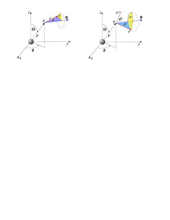
Figure 1: Geometry for electron-photon scattering. The left (right) panel refers to the situation before (after) scattering; all relevant angles are indicated. The direction of the spawned photon with energy $\epsilon^{\prime\prime}$ is also shown (note that this is only allowed for intermediate states with quantum number $n\geq 2$). The figure has only illustrative purposes and here all quantities are referred to an observer at rest with the star.

3 Resonant cross sections for photon-electron scattering

In strong magnetic fields the transverse momentum of a charge is not conserved upon scattering since the field can absorb or add momentum to the particle. The charge momentum parallel to the magnetic field, $p$, instead, is related to the parallel components of the photon momentum before and after the collision by the usual conservation law, which, in the ERF reads

$$p^{\prime} = \epsilon\,\cos\theta-\epsilon^{\prime}\,\cos\theta^{\prime}.$$ (3)

After the collision the particle is left in a state with principal quantum number $\ell\geq 0$ and energy $E^{\prime}_{\ell}\ =\ \sqrt{1+{p^{\prime}}^{2}+2\ell B}$. Energy and parallel momentum as measured in the ERF and in the frame where the recoiled electron is at rest, ERF^⋆, are then related by the Lorentz transformations

$$\sqrt{1+2\ell B} = E^{*}_{\ell}\ =\ \gamma^{\prime}\,(E^{\prime}_{\ell}-\beta^{\prime}\,p^{\prime})\qquad\quad{\rm and}\qquad\quad 0\ =\ p^{*}\ =\ \gamma^{\prime}\,(p^{\prime}-\beta^{\prime}\,E^{\prime}_{\ell}),$$ (4)

from which the velocity and energy of the excited particle in the ERF follows

$$\beta^{\prime} = \displaystyle{{p^{\prime}}\over{\sqrt{1+{p^{\prime}}^{2}+2\ell B}}}\,\,,\qquad\gamma^{\prime}\ =\ \displaystyle{{\sqrt{1+{p^{\prime}}^{2}+2\ell B}}\over{\sqrt{1+2\ell B}}}\,\,.$$ (5)

Finally, parallel momentum and energy conservation yields the final photon energy

$$\epsilon^{\prime} = \displaystyle{{\epsilon^{2}\,\sin^{2}\theta+2\epsilon-2\ell B}\over{1+\epsilon(1-\,\cos\theta\,\cos\theta^{\prime})+\sqrt{\,1+2\epsilon\,\cos\theta^{\prime}(\,\cos\theta^{\prime}-\,\cos\theta)+\epsilon^{2}(\,\cos\theta-\,\cos\theta^{\prime})^{2}+2\ell B\,\sin^{2}\theta^{\prime}}}}\,.$$ (6)

A strong magnetic field greatly affects the scattering cross section, but its effect is substantially different in the case the photon electric vector is parallel or perpendicular to $\vec{\cal B}$. For frequencies below $\omega_{B}$ the cross section of the extraordinary mode ($\perp$-mode) is greatly suppressed with respect to the Thomson value, $\sigma_{T}$ (Canuto, Lodenquai & Ruderman, 1971). Both polarization modes manifest, however, a singular behavior at nearly regular frequencies $\omega_{n}$, which correspond to excitations of the quantum Landau levels. In the frame where the electron is initially at rest and using the dimensionless variables defined in §2 the relativistic second order cross section for the transition from the ground to an arbitrary state $\ell$ is

$$\displaystyle{{d\sigma_{s\to s^{\prime}}}\over{d\Omega^{\prime}}} = \displaystyle{{3\sigma_{T}}\over{16\pi}}\,\displaystyle{{\epsilon^{\prime}}\over{\epsilon}}\,\displaystyle{{(2+\epsilon-\epsilon^{\prime})\,\exp{[-(\epsilon^{2}\,\sin^{2}\theta+{\epsilon^{\prime}}^{2}\,\sin^{2}\theta^{\prime})/2B}]}\over{[1+\epsilon-\epsilon^{\prime}-(\epsilon\,\cos\theta-\epsilon^{\prime}\,\cos\theta^{\prime})\,\cos\theta^{\prime}]}}\,\left|\,\sum_{n=0}^{\infty}\,\left[F_{n,-}^{(1)}+F_{n,+}^{(1)}+\left(F_{n,-}^{(2)}+F_{n,+}^{(2)}\right)\exp{(2i\Phi)}\right]\,\right|^{2}$$ (7)

(see equation [11] of Harding & Daugherty 1991 where some misprints have been corrected). Here $d\Omega^{\prime}=\sin\theta^{\prime}d\theta^{\prime}d\varphi^{\prime}$, the phase $\Phi$ depends on the difference $\varphi-\varphi^{\prime}$, and the complete expressions for the functions $F_{n,\pm}^{(k)}$ can be found in the Appendix of Harding & Daugherty (1991). The major complication in equation (7) derives from the presence of an infinite sum over all intermediate (virtual) states with principal quantum number $n$. In addition, the $F_{n,\pm}^{(k)}$ are complicated complex functions of $B,\,\epsilon$, $\epsilon^{\prime}$, $\theta\,,\theta^{\prime}$, $\varphi\,,\varphi^{\prime}$. They depend also on the initial and final photon polarization mode, $s,\,s^{\prime}$, and on the spin orientation of the electron in the intermediate state, i.e. spin-up (labelled by the index $+$) or spin-down (index $-$). Finally, if $\ell>0$, the form of these functions is different if the orientation of the electron spin in the final state is up ($f=1$) or down ($f=0$). If the final state is the ground state only spin down is allowed.

All the $F_{n,\pm}^{(1)}$ exhibit a divergent behaviour at the resonant energies

$$\epsilon_{n} = \displaystyle{{2nB}\over{1+\sqrt{1+2nB\sin^{2}\theta}}}\,.$$ (8)

while the $F_{n,\pm}^{(2)}$, which are obtained from $F_{n,\pm}^{(1)}$ by plane crossing symmetry replacement of variables (see again Harding & Daugherty, 1991), remain instead finite. Since, as mentioned earlier on, we are interested only in resonant scattering, this leads to a major simplification. Neglecting all non-resonant contributions in (7) when $\epsilon\simeq\epsilon_{n}$, which amounts to disregard both the $F_{n,\pm}^{(2)}$ and the non-resonant terms in the $F_{n,\pm}^{(1)}$, makes it possible to express the cross section as a infinite sum of separated terms

$$\displaystyle{{d\sigma_{s\to s^{\prime}}}\over{d\Omega^{\prime}}} = \sum_{n=1}^{\infty}\displaystyle{{d\sigma^{(n)}_{s\to s^{\prime}}}\over{d\Omega^{\prime}}}$$ (9)

where each resonant contribution is given by

$$\displaystyle{{d\sigma^{(n)}_{s\to s^{\prime}}}\over{d\Omega^{\prime}}} = \displaystyle{{3\sigma_{T}}\over{16\pi}}\,\displaystyle{{\epsilon^{\prime}}\over{\epsilon}}\,\displaystyle{{(2+\epsilon-\epsilon^{\prime})\,\exp{[-(\epsilon^{2}\,\sin^{2}\theta+{\epsilon^{\prime}}^{2}\,\sin^{2}\theta^{\prime})/2B]}}\over{[1+\epsilon-\epsilon^{\prime}-(\epsilon\,\cos\theta-\epsilon^{\prime}\,\cos\theta^{\prime})\,\cos\theta^{\prime}]}}\,\left|\,F_{n,+}^{(1)}\ +\ F_{n,-}^{(1)}\,\right|^{2}.$$ (10)

The quantities $F_{n,\pm}^{(1)}$ are independent on $\varphi$ and have the general form

$$F_{n,\pm}^{(1)} = \left(\displaystyle{{1+E_{n}}\over{2E_{n}}}\right)\,\displaystyle{{\,T^{n,\ell}_{\pm}(\epsilon,\epsilon^{\prime},\theta,\theta^{\prime},B;\,s,s^{\prime},f)}\over{1+\epsilon-E_{n}}}$$ (11)

where

$$E_{n} = \sqrt{1+\epsilon^{2}\,\cos^{2}\theta+2nB}$$ (12)

is the energy of the electron in the intermediate state. As discussed in §2, we restrict our treatment to situations in which scattering occur only via excitation of intermediate states $n\leq 2$, i.e. we only consider the first two resonant terms in equation (10); the corresponding expression for $\,T^{n,\ell}_{\pm}$ are given explicitly in the Appendix.

Actually, the divergence of the $F_{n,\pm}^{(1)}$, which occurs when the denominator $1+\epsilon-E_{n}$ vanishes, reflects an unphysical behaviour of the cross section and is merely a consequence of the fact that the expressions presented so far have been computed without accounting for the finite lifetime of the electron in the excited Landau levels. In a realistic situation, according to the Heisenberg principle, each excited level has an energy indeterminacy which is proportional to the inverse of the lifetime of the electron in that state, i.e. to the decay rate. This is standardly accounted for by introducing the natural line widths, which amounts to perform the substitution

$$E_{n}\ \to \ E_{n}-{i}\,\Gamma^{n}_{\pm}/2,$$ (13)

in the denominator of equation (11); here the $\,\Gamma^{n}_{\pm}$ are related to the relativistic decay rate out of the $n$-th intermediate state and their explicit expressions will be presented in §4. With this substitution, the functions (11) become

$$F_{n,\pm}^{(1)} = \left(\displaystyle{{1+E_{n}}\over{2E_{n}}}\right)\,\displaystyle{{\,T^{n,\ell}_{\pm}}\over{1+\epsilon-E_{n}+i\,\Gamma^{n}_{\pm}/2}}.$$ (14)

A more useful representation is obtained by replacing the Lorentzian that naturally arises from (14), with a $\delta$-function. By taking the limit

$$\lim_{\,\Gamma^{n}_{\pm}\to 0}\displaystyle{{\,\Gamma^{n}_{\pm}/2\pi}\over{(\epsilon-E_{n}+1)^{2}+(\,\Gamma^{n}_{\pm}/2)^{2}}} = \delta(\epsilon-E_{n}+1)$$ (15)

we obtain, after a lengthy but straightforward calculation,

$$\left|\,F_{n,+}^{(1)}+F_{n,-}^{(1)}\,\right|^{2} = \displaystyle{{\pi}\over{2}}\,\left(\displaystyle{{1+E_{n}}\over{E_{n}}}\right)^{2}\,\left[\displaystyle{{({\,T^{n,\ell}_{+}})^{2}}\over{\,\Gamma^{n}_{+}}}+\displaystyle{{({\,T^{n,\ell}_{-}})^{2}}\over{\,\Gamma^{n}_{-}}}+\displaystyle{{4\,\,T^{n,\ell}_{+}\,\,T^{n,\ell}_{-}}\over{\,\Gamma^{n}_{+}+\,\Gamma^{n}_{-}}}\right]\displaystyle{{E_{n}(\epsilon_{n})\,\delta(\epsilon-\epsilon_{n})}\over{\sqrt{1+2nB\sin^{2}\theta}}}\,.$$ (16)

We note that the factor $E_{n}(\epsilon_{n})/\sqrt{1+2nB\sin^{2}\theta}$ in eq. (16) arises because of the change in the argument of the $\delta$-function, from $\epsilon-E_{n}(\epsilon)+1$ to $\epsilon-\epsilon_{n}$. Ultimately it reflects the fact that the “effective” width of the scattering line profile near resonance is $\Gamma_{n}E_{n}(\epsilon_{n})/(2\sqrt{1+2nB\,\sin^{2}\theta})$ (see Harding & Daugherty, 1991).

Substituting back equation (16) into equation (10) and upon a trivial integration on $\varphi^{\prime}$, brings the $n$-th resonant term (10) in the form

$$\displaystyle{{d\sigma^{(n)}_{s\to s^{\prime}}}\over{d{\,\cos\theta\,}^{\prime}}} = {\cal D}^{(n)}_{s\to s^{\prime}}(B,\theta,\theta^{\prime})\,\delta(\epsilon-\epsilon_{n}),$$ (17)

where

$${\cal D}^{(n)}_{s\to s^{\prime}}=\displaystyle{{3\pi\sigma_{T}}\over{16}}\displaystyle{{(1+E_{n})^{2}}\over{E_{n}\sqrt{1+2nB\sin^{2}\theta}}}\,\displaystyle{{\epsilon^{\prime}\,(2+\epsilon-\epsilon^{\prime})\exp{[-(\epsilon^{2}\,\sin^{2}\theta+{\epsilon^{\prime}}^{2}\,\sin^{2}\theta^{\prime})/2B]}}\over{\epsilon[1+\epsilon-\epsilon^{\prime}-(\epsilon\,\cos\theta-\epsilon^{\prime}\,\cos\theta^{\prime})\,\cos\theta^{\prime}]}}\left[\displaystyle{{({\,T^{n,\ell}_{+}})^{2}}\over{\,\Gamma^{n}_{+}}}+\displaystyle{{({\,T^{n,\ell}_{-}})^{2}}\over{\,\Gamma^{n}_{-}}}+\displaystyle{{4\,\,T^{n,\ell}_{+}\,\,T^{n,\ell}_{-}}\over{\,\Gamma^{n}_{+}+\,\Gamma^{n}_{-}}}\right]\,,$$ (18)

and $\epsilon^{\prime}$ is given by equation (6). In the previous expression one can safely put $\epsilon=\epsilon_{n}$ since ${\cal D}^{(n)}_{s\to s^{\prime}}$ in multipled by $\delta(\epsilon-\epsilon_{n})$.

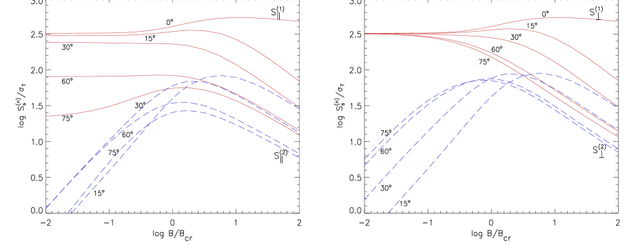
Figure 2: The resonance factors for the first (upper curves, solid red lines) and second (lower curves, dashed blue lines) intermediate Landau levels as a function of $\log B$; the $S^{(n)}_{s}$ are in unit of the Thomson cross section. Different curves are labelled by the value of the angle between the incident photon direction and the magnetic field. Left: ordinary photons. Right: extraordinary photons (note the weaker angular dependence in the latter case). Clearly, for a photon propagating parallel to the magnetic field only the first resonance exists and $S^{(2)}_{s}$ vanishes.

The $n$-th resonant term in the angle-integrated cross section is

$$\sigma^{(n)}_{s\to s^{\prime}} = {S}^{(n)}_{s\to s^{\prime}}(B,\theta;\ell,f)\delta(\epsilon-\epsilon_{n})\,,$$ (19)

where the integral

$${S}^{(n)}_{s\to s^{\prime}}(B,\theta;,\ell,f) = \int_{-1}^{1}{\cal D}^{(n)}_{s\to s^{\prime}}d({\,\cos\theta\,}^{\prime})$$ (20)

can be evaluated numerically. The $n$-th resonant term of the total cross section is then obtained by summing equation (19) over the polarization states of the scattered photon, $s^{\prime}$, and over the energy levels $\ell$, and the spin states, $f$, of the recoiled electron.

When $n=1$, the terms $\,S^{(1)}_{s\to s^{\prime}}$ and ${\cal D}^{(1)}_{s\to s^{\prime}}\,$ are not associated with a choice of different quantum states $\ell$ and $f$, because in this case it necessarily follows that $\ell=0$ and $f=0$. Therefore, for a photon with given initial polarization $s$, the first resonant term of the total cross section is simply given by the sum of two contributions, i.e.

$$\sigma^{(1)}_{s}(\epsilon,B,\theta) = \left[S^{(1)}_{s\to 1}(B,\theta;\,\ell=0,f=0)\ +\ S^{(1)}_{s\to 2}(B,\theta;\,\ell=0,f=0)\right]\delta(\epsilon-\epsilon_{1})\ =\ S^{(1)}_{s}(B,\theta)\,\delta(\epsilon-\epsilon_{1}).$$ (21)

Instead, the second resonant term of the total cross section, corresponding to the intermediate state $n=2$, must account for both final states $\ell=0,\,1$ and, if $\ell=1$, for two different orientations of the electron spin. Its expression is then

$$\sigma^{(2)}_{s}(\epsilon,B,\theta) = \left\{\left[S^{(2)}_{s\to 1}(B,\theta;\ell=0,f=0)\ +\ S^{(2)}_{s\to 2}(B,\theta;\ell=0,f=0)\right]\ +\ \right.$$

$$\left.\left[S^{(2)}_{s\to 1}(B,\theta;\ell=1,f=0)\ +\ S^{(2)}_{s\to 2}(B,\theta;\ell=1,f=0)\right]\ +\ \right.$$

$$\left.\left[S^{(2)}_{s\to 1}(B,\theta;\ell=1,f=1)+S^{(2)}_{s\to 2}(B,\theta;\ell=1,f=1)\right]\right\}\delta(\epsilon-\epsilon_{2})\ =\ S^{(2)}_{s}(B,\theta)\,\delta(\epsilon-\epsilon_{2})\,.$$

Finally, the total cross section is obtained by adding the different resonant terms

$$\sigma_{s}(\epsilon,B,\theta) = \sigma^{(1)}_{s}(\epsilon,B,\theta)+\sigma^{(2)}_{s}(\epsilon,B,\theta)=\sum_{n=1}^{2}\,S_{s}^{(n)}(B,\theta)\,\delta(\epsilon-\epsilon_{n}).$$ (23)

The eight functions $\,S^{(n)}_{s\to s^{\prime}}\,$ which appear in equations (21)-(3) are the fundamental ingredients for any computational investigation of photon diffusion in strong magnetized plasmas. In particular, when performing Monte Carlo simulations, proper combinations of these expressions can be used to evaluate the probability of transition between different states.

Figure 2 illustrates the dependence of the functions $S^{(1)}_{s}$ and $S^{(2)}_{s}$ on the magnetic field strength for both polarization states and different incident photon direction. The non-relativistic limit tangent to the low $B$-field limit of each curve and takes the form

$$S_{\perp}^{(1)} \sim \displaystyle{{3\pi}\over{8\alpha}}(2+B\,\cos^{2}\theta)\,,\hskip 28.45274ptS_{\parallel}^{(1)}\sim\displaystyle{{3\pi}\over{8\alpha}}(2\,\cos^{2}\theta+B)$$

$$S_{\perp}^{(2)} \sim \displaystyle{{3\pi}\over{2\alpha}}B\,\sin^{2}\theta\,,\hskip 50.50346ptS_{\parallel}^{(2)}\sim\displaystyle{{3\pi}\over{2\alpha}}B\,\sin^{2}\theta(B+\,\cos^{2}\theta)\,,$$

where $\alpha=1/137$ is the fine structure constant. In the ultra-relativistic limit no simple analytical expansion can be derived. Approximate expressions, which hold for $\theta\neq 0$, are $S^{(1)}_{\parallel}\simeq S^{(1)}_{\perp}\propto 1/(1+2\sqrt{B\,\sin^{2}\theta}\,)$ and $S^{(2)}_{\parallel}\simeq S^{(2)}_{\perp}\propto 1/(1+\sqrt{B\,\sin^{2}\theta}\,)$. As it can be seen, relativistic corrections are already $\sim 10\%$ at ${\cal B}\sim 0.1\,{\cal B}_{cr}$ for photons with large values of the incident angle $\theta$ (see Figure 2). Furthermore, we may note that the number of excitations of the second Landau level, totally negligible in the weak $B$ limit, becomes sizable in moderately relativistic regimes.

This result is more evident in Figure 3 (left panel), where we show the ratio between the second resonant term and the total cross section in the case of unpolarized incident photons, obtained averaging over ordinary and extraordinary modes ($s=1,\,2)$. As it can be seen, in strong magnetic fields a non-negligible fraction of collisions can excite electrons to the higher Landau level ($n=2$). It is also worth noticing that, when $n=2$, de-excitation of the electron to $\ell=1$ state is generally more likely than the direct transition to the ground level, as it can be seen from the right panel in Figure 3. Only for magnetic field strengths largely exceeding the critical quantum limit, the two transitions are have comparable probabilities. This has important consequences on the transfer problem, since it implies that collisions involving the intermediate state $n=2$ lead more frequently to the creation of extra photons as the electron returns to the ground level. In other words, the resonant magnetic scattering may not conserve the total photon number.

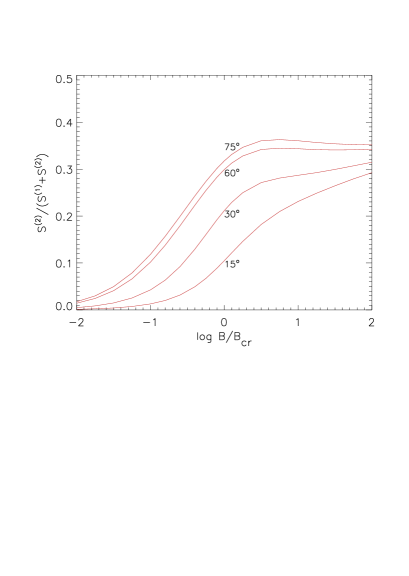
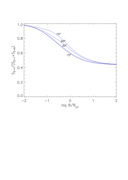
Figure 3: Left: The ratio $S^{(2)}/(S^{(1)}+S^{(2)})$ versus the magnetic field strength for three different scattering angles. The functions $S^{(n)}$ are obtained by summing over the two initial photon polarization states, i.e. $S^{(n)}=S^{(n)}_{1}+S^{(n)}_{2}$. Right: The $2\to 1$ transition probability versus magnetic field strength.

4 Transition Rates

For the sake of completeness, in this section we present the explicit expressions for the transition rates and for the natural line widths $\,\Gamma^{n}_{\pm}$. The differential transition rates (number of decays per second and per sterad) for electrons with initial spin up ($+$) or down ($-$) were derived in a general form by Daugherty & Ventura (1978) and Herold, Ruder & Wunner (1982) (see also Latal, 1986; Baring, Gonthier & Harding, 2005). Here we will use the derivation presented by Herold, Ruder & Wunner (1982), by focussing only on those cases which are of immediate relevance to the present investigation. In this respect, we note that, while performing a Monte Carlo simulation, the transitions rates have a twofold role. First, as discussed in § 3, they fix the natural width of the Landau levels, and therefore enter directly into the numerical computation of the resonant scattering cross section. Second, as we will see in § 5, they determine the properties of the photons emitted by successive de-excitations when, in Landau-Raman scattering the electron is left in an excited state $\ell>0$. In practice, in the particular case we are discussing (i.e. only levels up to $n=2$ can be excited), it is the differential transition rate $dR_{\pm}^{\,1\to 0}/d\Omega$ (see equation 27 below) that fixes the properties of the photon which is emitted through the decay of an electron from $\ell=1$ to the ground level.

The cross sections discussed in the previous sections have been computed in the frame in which the electron is at rest before scattering (ERF, see §3), and the parallel component of the momentum in the intermediate state $n$ is $p=\epsilon_{n}\,\cos\theta$. However, in this section we find more convenient to proceed by first introducing the transition rates and line widths $\,\widetilde{\Gamma}_{\pm}^{n}\,$ as computed in the reference frame ERF^⋆⋆  in which the electron is momentarily at rest in the virtual state $n$, and then to transform them back in the ERF. In fact, in the ERF^⋆⋆ the equations governing the de-excitation and the consequent photon emission take their simpler form. Furthermore, in this section we will indicate with $\,E_{n}\,$ and $\,E_{\ell}\,$ the energy of the electron in the state $n$, $\ell$, and with $\epsilon_{e}$ and $\theta_{e}$ the energy and direction (wrt the magnetic field) of the emitted photon, respectively. All these quantities are computed in the ERF^⋆⋆.

In the ERF^⋆⋆, the energy of an electron which is excited to the level $n$ is therefore

$$E_{n} = \sqrt{1+2nB}\,.$$ (24)

By applying again energy and parallel momentum conservation we obtain the energy of the electron de-excited to the level $\ell$ and that of the emitted photon

$$E_{\ell} = E_{n}\ -\ \epsilon_{e}\ =\ \sqrt{1+2\,\ell\,B+\epsilon_{e}^{2}\cos^{2}\theta_{e}}$$ (25)

$$\epsilon_{e} = \displaystyle{{2(n-\ell)B}\over{E_{n}+\sqrt{1+2B(n\cos^{2}\theta_{e}+\ell\sin^{2}\theta_{e})}}}$$ (26)

respectively.

The differential rate for transitions between a generic level $n>0$ and the ground state $\ell=0$, as given by Herold, Ruder & Wunner (1982), takes the form

$$\displaystyle{{dR_{\pm}^{\,n\to 0}}\over{d\Omega}} = \displaystyle{{\alpha mc^{2}}\over{4\pi\hbar}}\,\displaystyle{{\epsilon_{e}\,\exp{(-Z)}\,Z^{n-1}}\over{(n-1)!\,E_{n}\,(E_{n}-\epsilon_{e}\sin^{2}\theta_{e})}}\left\{\displaystyle{{Z}\over{n}}\,\left[\displaystyle{{}\over{}}2nB-\epsilon_{e}\,(E_{n}\,\mp\,1)\right]\langle\sin^{2}\theta_{e},0\rangle\ +\ \right.$$ (27)

$$\left.\ +\ \left[\displaystyle{{}\over{}}2nB-\epsilon_{e}\,(E_{n}\,\pm\,1)\right]\,\langle\cos^{2}\theta_{e},1\rangle\ +\ 2\epsilon^{2}\,\cos^{2}\theta_{e}\langle\sin^{2}\theta_{e},0\rangle\right\},$$

where $Z=\epsilon_{e}^{2}\sin^{2}\theta_{e}/2B$. The angular factors in “$\langle\,\rangle$” refer to two possible linear polarization states $s=1,2$. The rate for transition from $n=2$ to $\ell=1$ is

$$\displaystyle{{dR_{\pm}^{2\to 1}}\over{d\Omega}} = \displaystyle{{\alpha mc^{2}}\over{4\pi\hbar}}\,\displaystyle{{\epsilon_{e}\,\exp{(-Z)}}\over{\,E_{n}\,(E_{n}-\epsilon_{e}\sin^{2}\theta_{e}\,)\,}}\left\{Z\,\left[[\displaystyle{{}\over{}}4B-\epsilon_{e}\,\,(E_{n}\,\mp\,1)]{(Z-2)^{2}}/{2}\ +\ \right.\right.$$ (28)

$$\left.+\ \displaystyle{{}\over{}}4B-\epsilon_{e}\,(E_{n}\,\pm\,1)+4B\,(2Z-3)\right]\,\langle{\sin^{2}\theta_{e}},0\rangle\ +\ \left[\displaystyle{{}\over{}}[\,4B-\epsilon_{e}\,(E_{n}\,\pm\,1)]\,(Z-1)^{2}\ +\ \right.$$

$$\left.+\ [\displaystyle{{}\over{}}4B-\epsilon_{e}\,(E_{n}\,\mp\,1)]\,Z^{2}/2\right]\,\langle\cos^{2}\theta_{e},{1}\rangle\ +\ \left.2\epsilon_{e}^{2}\,\cos^{2}\theta_{e}(Z^{2}-2Z+2)\,\langle{\sin^{2}\theta_{e},\,0}\rangle\displaystyle{{}\over{}}\right\}.$$

Since we are considering only the first two resonances, the two previous expressions are all we need in order to evaluate the natural widths and photon emission following Landau-Raman scattering (see §5).

Total rates can be obtained by integrating over the solid angle and summing over the two polarization states $s$ of the emitted photon, and in general take the form

$$R_{\pm}^{n\to\ell} = 2\pi\int_{-1}^{1}\,\sum_{s=1}^{2}\,\displaystyle{{dR^{n\to\ell}_{\pm}}\over{d(\cos\theta_{e})}}\,d(\cos\theta_{e})\,.$$ (29)

The reciprocal of the transition rate gives the mean lifetime of the electron in the excited Landau level. Then, due the Heisemberg principle, each term $R_{\pm}^{n\to\ell}$ is proportional to the energy width for the particular transition $n\to\ell$. The total energy width of the $n$-th level is therefore obtained by summing over all contributions associated with level $n$

$$\widetilde{\Gamma}_{\pm}^{n} = \displaystyle{{\hbar}\over{m_{e}c^{2}}}\sum_{k=0}^{n-1}R^{n\to k}_{\pm}\,.$$ (30)

As previously stated, these expressions are valid in the reference frame in which the excited electron is at rest, ERF^⋆⋆. In order to obtain the energy widths $\,\Gamma^{n}_{\pm}$ that must be used in the expressions given in § 3, we need to perform a Lorentz transformation back to the ERF. This gives

$$\,\Gamma^{n}_{\pm} = \displaystyle{{\sqrt{1+2nB}}\over{\sqrt{1+\epsilon_{n}^{2}\,\cos^{2}\theta+2nB}}}\,\,\widetilde{\Gamma}_{\pm}^{n}\,,$$ (31)

where $\epsilon_{n}$ and $\theta$ are the incident photon energy (equation [8]) and direction. Figure 4 shows the dependence on the magnetic field strength of the total energy widths for the first two Landau levels, $\widetilde{\Gamma}_{\pm}^{1,2}$, in the range $10^{-3}\leq{\cal B}/{\cal B}_{cr}\leq 10^{2}$. For weak fields they are proportional to $B^{2}$ (in particular $\widetilde{\Gamma}^{1}_{-}\sim 4\alpha B^{2}/3$), except for the spin flip transition for which $\widetilde{\Gamma}^{1}_{+}\sim 2\alpha B^{3}/3$ (e.g. Herold, Ruder & Wunner, 1982; Latal, 1986). Similarly to what happens for the cross sections, remarkable deviations from the simple, non-relativistic power-law dependence appears at $B>0.1$. We note that in the strong field limit all energy widths have a similar dependence on the field strength, $\sim 0.4\alpha\sqrt{B}$, a result similar to that found by Latal (1986) for the total transition rate. The limiting behaviours of $\widetilde{\Gamma}_{\pm}^{1}$ can be usefully checked against those derived by Baring, Gonthier & Harding (2005) who obtained an analytical form (in terms of a series of elementary functions) for the spin-dependent transition rates $R^{n\to 0}_{\pm}$. In fact, for $n=1$, it follows from eq. (30) that $\widetilde{\Gamma}_{\pm}^{1}=(\hbar/m_{e}c^{2})R^{1\to 0}_{\pm}$. As noticed by Baring, Gonthier & Harding (2005), their weak field limit coincides with those derived (analitycally) by Latal (1986) and discussed above. In the ultra-relativistic limit, on the other hand, one gets $\widetilde{\Gamma}^{1}_{-}\sim\widetilde{\Gamma}^{1}_{+}\sim\alpha(1-1/\mathrm{e})(B/2)^{1/2}\sim 0.45\alpha\sqrt{B}$, close to the $B\gg 1$ limit given above. A direct numerical comparison of our result for $\widetilde{\Gamma}_{\pm}^{1}$ with that of Baring, Gonthier & Harding (2005) shows that the fractional difference is below 10% for $B<100$, with the largest deviations appearing at large $B$.

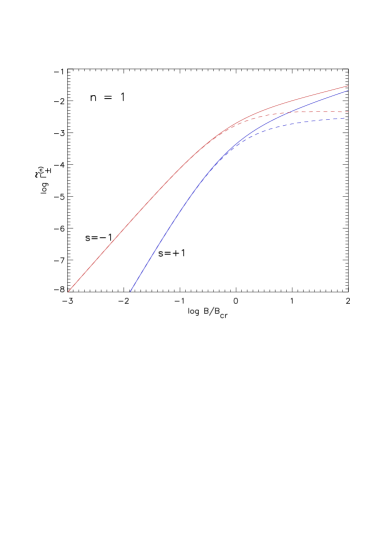
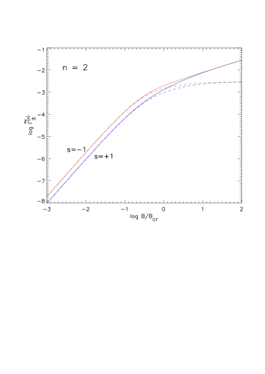
Figure 4: Energy widths of the Landau levels (in units of $m_{e}c^{2}$) for the two spin orientations as a function of the magnetic field strength. Left: $n=1$. Right: $n=2$. In each panel the full lines refer to the widths as computed in the excited electron frame [eq. (30)] and the dashed lines to the same quantities but referred to the ERF [eq. (31)] for $\cos\theta=\pm 1$, i.e. in the case in which the incoming photon is parallel to $\mathbf{B}$.

5 Photon spawning

As discussed in the previous sections, some scatterings occur at the second resonance and excite the electron in the intermediate state $n=2$. In order to have a significant number of second harmonic excitations the magnetic field must be sufficiently intense, say $B\ \ga\ 0.05$ (${\cal B}\ga 2.2\times 10^{12}$ G; see Figure 3 ). Moreover, the incoming photon must have an energy $\epsilon=\epsilon_{2}\approx 2B$. The two conditions together require that a significant number of photons with energy $\hbar\omega\ga 50$ keV are present in the magnetosphere. We do not expect such high-energy photons to be emitted directly by the stellar surface, which temperature, as inferred by observed X-ray spectra, is $\sim 0.5$–1 keV, but it must be noted that, if electrons are relativistic, the photon energy as seen by the moving particle will be amplified by a factor $\sim\gamma$. Besides, repeated collisions populate the hard tail of the spectrum and may provide photons of the required energy.

Once an electron is excited to the second Landau level, it is more likely left after scattering in the $\ell=1$ rather than in the $\ell=0$ state (see § 3 and Figure 3). This implies that an additional photon will be produced by the prompt radiative de-excitation $1\to 0$. In general, the transition rate depends also on the rate at which collisions populate the $\ell=1$ level. The excitation rate due to Coulomb collisions is (Bonazzola, Heyvaerts & Puget, 1979)

$$R_{coll} \approx 3\times 10^{10}\left(\displaystyle{{n_{e}}\over{10^{21}{\rm cm}^{-3}}}\right)T^{-3/2}\ {\rm s}^{-1}\quad\approx\quad 1.6\times 10^{6}\left(\displaystyle{{n_{e}}\over{10^{21}{\rm cm}^{-3}}}\right)\,B^{-3/2}\ {\rm s}^{-1}\,,$$

where the second (approximate) equality follows from the requirement that it has to be $kT\sim\hbar\omega_{B}$ for the collision to excite the first Landau level. As noticed by Araya & Harding (1999), in a strongly magnetized, low-density plasma $R_{coll}$ is negligible when compared to the radiative cyclotron rate

$$R_{rad} \approx 10^{18}\,B^{q}\ {\rm s}^{-1}$$ (32)

where the exponent $q$ varies in the range 1/2–2 (see §4). The population of the excited Landau levels is, therefore, solely regulated in the present case by magnetic Compton scattering. The large value of $R_{rad}$ justifies the assumption that electrons remain in the ground level. In fact, the typical time between two scatterings is $\approx(n_{e}\sigma c)^{-1}\approx L/(\tau c)\approx 10^{-5}\,{\rm s}\gg 1/R_{rad}$, where the lengthscale $L$ is a few star radii and the scattering depth $\tau\approx 1$ (see paper I). In a sense, one may view Raman scattering at the second resonance, and the ensuing, quick radiative de-excitation to the $\ell=0$ level (photon spawning) as more akin to double Compton scattering (e.g. Gould, 1984) rather than to absorption followed by the emission of two photons.

As discussed in § 4, the de-excitation of an electron which is initially at rest in the $\ell=1$ level with energy $E=\sqrt{1+2B}$ produces a photon with energy

$$\epsilon_{e} = \displaystyle{{E-\sqrt{{E}^{2}-2B\,\sin^{2}\theta_{e}}}\over{\,\sin^{2}\theta_{e}}}\ =\ \displaystyle{{2B}\over{\sqrt{1+2B}+\sqrt{1+2B\,\cos^{2}\theta_{e}}}}\,,$$ (33)

as computed in its rest frame. The rate at which photons are emitted is given by equation (29) with $n=1,\ \ell=0$, and, when performing a Monte Carlo simulation, the differential form (27) can be used to derive, on a probabilistic ground, the direction of the emitted photon (i.e. the angle $\theta_{e}$, emission is isotropic in $\phi_{e}$). Once again, we stress that care must be payed to the frame in which these quantities are evaluated. In fact, the emission angle $\theta_{e}$ and the photon energy $\epsilon_{e}$ introduced above, are both referred to the rest frame of the recoiled electron, while in applications they need to be evaluated in the stellar frame (LAB). This is readily done by means of a Lorentz transformation. In this respect, we note that the parallel momentum of the recoiled electron is in the LAB

$$p^{\prime} = \gamma\beta+\epsilon\,\mu-\epsilon^{\prime}\,\mu^{\prime}$$ (34)

where $\epsilon$ and $\mu$ are the photon energy and the cosine of the propagation angle with respect to the magnetic field, both measured in the stellar frame, and, again, unprimed (primed) variables refer to quantities before (after) the scattering. The corresponding velocity and the Lorentz factor are $\,\beta^{\prime}=p^{\prime}/\sqrt{1+{p^{\prime}}^{2}+2B}\,$ and $\,\gamma^{\prime}=\sqrt{1+{p^{\prime}}^{2}+2B}/\sqrt{1+2B}\,$ respectively (see §3), from which we obtain

$$\cos\theta_{e}^{(L)} = \displaystyle{{\cos\theta_{e}+\beta^{\prime}}\over{1+\beta^{\prime}\cos\theta_{e}}}$$ (35)

and

$$\epsilon_{e}^{(L)} = \gamma^{\prime}\epsilon_{e}\left(1+\beta^{\prime}\cos\theta_{e}\right)\,;$$ (36)

here the index $(L)$ denotes the photon energy and propagation angle as measured in the stellar frame to distinguish them from the same quantities but referred to the recoiled electron frame.

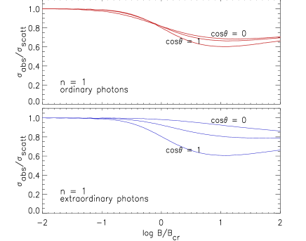
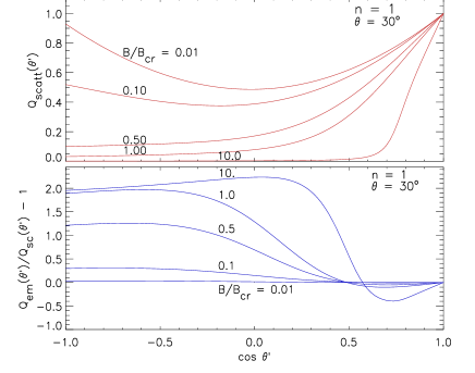
Figure 5: Left: the ratio $\sigma_{abs}/\sigma_{s}$ versus the magnetic field strength for ordinary (upper panel) and extraordinary (lower panel) photons, and three different directions of the incident photon, $\,\cos\theta=0,0.5,1$. Right: the angular distribution of scattered photons (upper panel) for a given incident photon direction $\theta=30^{\circ}$. The lower panel shows the fractional difference between emission and scattering, $(Q_{e}-Q_{s})/Q_{s}$. Each curve is labelled by the magnetic field strength.

6 Absorption-emission vs. scattering

As noted by Harding & Daugherty (1991) and Araya & Harding (1999), in the non-relativistic regime the on-resonance second order scattering process $\,\gamma+e\to\gamma^{\prime}+e^{\prime}\,$ is well approximated by the sequence of two separated first order processes: photon absorption, $\,\gamma+e\to e^{*}$, immediately followed by photon emission $\,e^{*}\to e^{\prime}+\gamma^{\prime}$. Because of its much simpler form, one would like to use the cyclotron absorption cross section instead of the cumbersome QED scattering cross section in numerical work. It is therefore of interest to explore the conditions under which absorption plus emission reproduces relativistic resonant scattering with reasonable accuracy.

In the ERF, summed over the final spin states, the angle-averaged absorption cross section can be written as (Daugherty & Ventura, 1978)

$$\sigma_{abs}^{(n)}({\parallel,\perp}) = \displaystyle{{3\pi\sigma_{T}}\over{4\alpha}}\displaystyle{{\exp{(-Z)}Z^{n-1}}\over{(n-1)!\sqrt{1+2nB\,\sin^{2}\theta}}}\left[1\ -\ \displaystyle{{\epsilon_{n}}\over{nB}}\,\langle\,\sin^{2}\theta,0\rangle\right]\delta{(\epsilon-\epsilon_{n})},$$ (37)

where the angular factor $\langle\,\sin^{2}\theta,0\rangle$ refers to the two linear polarizations ($\parallel,\ \perp$) of the incident photon, $Z=\epsilon^{2}_{n}\,\sin^{2}\theta/2B$, and the cyclotron harmonic energy $\,\epsilon_{n}\,$ is equal to the scattering resonant energy (see equation [8]).

The reliability and the limits of validity of this approach can be assessed by directly comparing equation (37) with the scattering cross sections (equations [21] and [3]), since these expressions are all explicitly written in terms of a $\delta$-function of the same argument. Figure 5 (left panel) shows the ratio of the absorption to the scattering cross sections for $n=1$ and both ordinary and extraordinary photons in the range $-2\leq\log B\leq 2$ and three different directions of the incident photon (corresponding to $\,\cos\theta=0,0.5,1$). The agreement is very good up to $B\sim 0.1$ for both polarization modes and deviations are within $\sim 20\%$ up to $B\sim 1$. However, this does not imply that the two descriptions of the photon-electron interaction are to be regarded as equivalent for $B\la 1$. To claim this, one should prove that they produce also the same angular redistribution of radiation in the final state. The angular distribution of the scattered photons is given (in the ERF) by equation (18) once $B$ and $\theta$ are fixed, while that of emitted photons by equation (27). The latter is evaluated in the zero-momentum frame of the excited electron, exhibits forward-backward symmetry, and lacks any information on the incoming photon. However, in the case under examination, the electron has been excited by the absorption of a photon with parallel momentum $\epsilon_{n}\cos\theta$. In order to compare the two angular distributions the transition rate must be properly transformed to the ERF (Araya & Harding, 1999), or, alternatively, it should be computed ab initio in the ERF, by exploiting the general expressions derived in Latal (1986) and valid for an arbitrary value of the electron parallel momentum. Since $p=\epsilon_{n}\,\cos\theta$, this clearly introduces a dependence on the incoming photon kinematical quantities in the transition rate.

Figure 5 (right) shows the angular distribution $\,Q_{s}(\theta^{\prime})\,$ of the scattered photons (upper panel) for $n=1$, a representative value of the incident photon angle, $\theta=30^{\circ}$, and different values of the magnetic field, $0.01\leq B\leq 10$. $\,Q_{s}\,$ has been computed by normalizing equation (18) to its maximum value, which occurs at $\theta^{\prime}=0$ and is the same for any $B$. Photons are more and more forward-scattered as the field increases. We verified that, as expected, this asymmetry strongly increases for $\theta\sim 0$ and $\theta\sim 180^{\circ}$, while the curves become symmetric for $\theta=90^{\circ}$. The lower panel shows instead (again, for $n=1$) the fractional difference between $\,Q_{s}(\theta^{\prime})\,$ and the analogous quantity for emission $\,Q_{e}(\theta^{\prime})\,$ (here $\theta^{\prime}\equiv\theta_{e}$), obtained normalizing the Lorentz-transformed transition rate (27). It is interesting to note that in this case the forward beaming is entirely due the relativistic Lorentz boosting in going from the ERF^⋆⋆ to the ERF. As the plot shows, there are significant differences in the angular distributions even at magnetic field below $0.1{\cal B}_{cr}$. This means that photon-electron scattering can be safely treated as the superposition of absorption and emission only for resonant photon energies $\la 10$ keV.

Similar results are obtained for transitions involving higher Landau levels, although in this case sensible differences arise even for lower magnetic field strengths. However, when $n>1$ major complications arise because of the necessity to discriminate transitions toward final levels different from the ground state, and to account for the possible changes of the photon polarization and electron spin orientation.

7 Scattering probability

Let us assume that a photon propagates in a strongly magnetized medium populated by electrons with a one-dimensional relativistic velocity distribution along the magnetic field direction

$$\displaystyle{{dn_{e}}\over{d\beta}} = \gamma^{3}n_{e}f_{e}(\vec{r},\gamma\beta)\,,$$ (38)

where $\,f_{e}=n_{e}^{-1}dn_{e}/d(\gamma\beta)\,$ is the momentum distribution function and $\,n_{e}(\vec{r})\,$ is the charge number density. As discussed in §5, all electrons can be taken to be initially in the ground Landau level. Having in mind the results obtained in Section 3, equation (23), the optical depth after a photon has travelled an infinitesimal distance $\,d\ell\,$ is

$$d\tau_{s} = d\ell\int_{\beta_{min}}^{\beta_{max}}d\beta\,\displaystyle{{dn_{e}}\over{d\beta}}\,(1-\beta\mu)\,\sigma_{s}=$$ (39)

$$= d\ell\sum_{n=1}^{2}\int_{\beta_{min}}^{\beta_{max}}d\beta\,n_{e}(\vec{r})\,\gamma^{3}\,f_{e}(\vec{r},\gamma\beta)\,(1-\beta\mu)\,S_{s}^{n}\,\delta\left[\gamma(1-\beta\mu)\epsilon^{(L)}-\epsilon_{n}\right],$$

in which $\,[\beta_{min},\beta_{max}]\,$ is the charge velocity spread and $\,\mu\,$ is the cosine of the propagation angle with respect to the magnetic field in the stellar frame (LAB). The latter quantity is related to the same angle as measured in the ERF by the usual transformations

$$\,\cos\theta = \displaystyle{{\mu-\beta}\over{1-\beta\mu}}\,,\qquad\,\sin\theta\ =\ \displaystyle{{\sqrt{1-\mu^{2}}}\over{\gamma(1-\beta\mu)}}\,.$$ (40)

The factor $\,(1-\beta\mu)\,$ in the integral (39) appears because of the change of reference between ERF and LAB, and, for the sake of clarity, the argument of the $\delta$-function has been explicitly written in terms of the energy $\epsilon^{(L)}$ measured by an observer at rest in the LAB.

The integral (39) can be readily performed exploiting the well-known properties of the $\delta$-function. Denoting by $\,{\beta^{(n)}_{k}}\,(k=1,2)$ the two roots (for each $n$) of the quadratic equation $\gamma(1-\beta\mu)\epsilon^{(L)}-\epsilon_{n}=0$, the $\delta$-function in energy can be transformed into a $\delta$-function in velocity by

$$\delta[\gamma(1-\beta\mu)\epsilon^{(L)}-\epsilon_{n}] = \sum_{k=1}^{2}\displaystyle{{\delta(\beta-{\beta^{(n)}_{k}})}\over{\left|\gamma^{3}\,g({\beta^{(n)}_{k}})\,\right|}}$$ (41)

where

$$g(\beta)\, \ =\ \displaystyle{{(\mu-\beta\,)\,\epsilon_{n}}\over{\sqrt{\gamma^{2}\,(1-\beta\,\mu)^{2}+2nB\,(1-\mu^{2})}}}\,$$ (42)

$${\beta^{(n)}_{k}} \ =\ \displaystyle{{1}\over{m^{2}+\mu^{2}}}\left[\mu\ \pm\ m\,\sqrt{m^{2}+\mu^{2}-1}\right]$$ (43)

$$m \ =\ \displaystyle{{nB}\over{\epsilon_{n}}}\left|1\ -\ \displaystyle{{\epsilon_{n}^{2}\,(1-\mu^{2})}\over{2nB}}\right|\,.$$ (44)

It is worth noticing that with this transformation the role played by the resonant photon is replaced by that of a pair of resonant electrons selected among all charges of the distribution. Accordingly, the elementary optical depth (39) for a photon with initial polarization state $s=(1,2)$, becomes

$$d{\tau}_{s} = {n_{e}}d\ell\,\sum_{n=1}^{2}\,\sum_{k=1}^{2}\,\displaystyle{{(1-\mu\,\beta_{k}^{(n)})\,f_{e}(\vec{r},\gamma{\beta^{(n)}_{k}})\,S_{s}^{(n)}(B,\theta(\mu,{\beta^{(n)}_{k}}))}\over{|\,g({\beta^{(n)}_{k}})\,|}}\ =\ {n_{e}}\,d\ell\,\sum_{n=1}^{2}\,A^{(n)}_{s};$$ (45)

the quantities $\,A^{(n)}_{s}\,$ are implicitly defined by equation (45), and we made evident the dependence of the resonant factors $S_{s}^{(n)}$, which are computed in the ERF, on the LAB variables.

Once energy, polarization and initial photon direction are fixed, equation (45) can be integrated numerically along the optical path until a scattering, if any, occurs. As it is apparent from equation (42), scattering may occur only when the roots ${\beta^{(n)}_{k}}$ are real, i.e. only where $\,h(r,\mu)\equiv m^{2}+\mu^{2}-1\geq 0$. Since the function $h$ depends only on position and photon direction, at every point in the magnetosphere the previous condition discriminates those pairs of energy and angle for which scattering is possible.

8 Conclusions

Recent models of spectral formation in magnetars called renewed attention on electron-photon scattering in the presence of ultra-strong magnetic fields. The complete expression for the QED cross section is known since long (e.g. Harding & Daugherty, 1991) but its practical application in the relativistic regime is numerically challenging. In many astrophysical problems, including the one which motivated us, it is reasonable to assume that scattering occurs only at resonance, i.e. when the incident photon frequency equals the cyclotron frequency (or one of its harmonics). Restricting to resonant scattering introduces a major simplification, and here we presented explicit expressions for the magnetic Compton cross section in this particular case. Our main goal has been to provide a complete, workable set of formulae which can be used in Monte Carlo simulations of photon scattering in strongly magnetized media.

Our results are fairly general and can be applied to resonant photon scattering under a variety of conditions. In particular, no assumption is made on the field strength. Having in mind applications to spectral modelling in the $\,\sim 0.1$–200 keV range, resonant scattering necessarily occurs where $\,{\cal B}/{\cal B}_{cr}\la 1$. Under these conditions, and although the expressions we derived are still valid for $\,{\cal B}/{\cal B}_{cr}>1$, we restricted to the case in which the electron is excited at most up to the second Landau level. We find that deviations from the non-relativistic limit in both the first and second resonant contributions to the cross section become significant for $\,{\cal B}/{\cal B}_{cr}\ga 0.1$. The probability that scattering occurs at the second resonance, which is negligible below $\,{\cal B}/{\cal B}_{cr}\la 0.01$, becomes sizeable at higher $B$ and, depending on the scattering angle, it can be up to $\,\sim 30\%\,$ for $\,{\cal B}\sim{\cal B}_{cr}$. In case the second Landau level is excited, its is more likely that the recoiled electron is left in the first than in the ground level with the ensuing emission of a new photon (spawning). Using our results for the cross section together with known expressions for the transition rates, we checked under which conditions resonant Compton scattering can be treated as the combination of two first-order processes, photon absorption followed by emission. While the scattering and absorption cross sections differ by at most $\,\sim 20\%\,$ for $\,{\cal B}\la{\cal B}_{cr}$, the angular distribution of the scattered/emitted photons shows deviations already at $\,{\cal B}\sim 0.1{\cal B}_{cr}$. Finally, having in mind the implementation in a Monte Carlo code (Nobili, Turolla & Zane, in preparation), we presented an explicit derivation of the scattering optical depth along the photon path.

Appendix A

The expressions below explicitly give the functions $T_{\pm}^{n\to\ell}(\epsilon,\epsilon^{\prime},\theta,\theta^{\prime},B;s,s^{\prime},f)$ introduced in equation (11) for the relevant values of $n$ and $\ell$. In the following, to simplify notation, only the dependence on $f$ is shown in the argument: $f=0$ refers to the no-flip and $f=1$ to the flip case.

$$T_{+}^{1\to 0}(0) = \displaystyle{{\epsilon\epsilon^{\prime}}\over{(2+\epsilon)^{2}}}\left[\displaystyle{{G\,}\over{\Omega}}\,({\cal M}_{1}\,\,\cos\theta-{\cal M}_{3}\,\,\sin\theta)+\,\sin\theta^{\prime}\,({\cal M}_{0}\,\,\sin\theta-{\cal M}_{2}\,\,\cos\theta)\right]$$

$$T_{-}^{1\to 0}(0) = \displaystyle{{1}\over{(2+\epsilon)^{2}}}\left[\displaystyle{{H\,\epsilon^{\prime}\,\sin\theta^{\prime}}\over{2B\Omega}}\,(2B\,{\cal M}_{2}\,+{\cal M}_{0}\,\epsilon^{2}\,\sin\theta\,\cos\theta)+(2B{\cal M}_{1}\,+{\cal M}_{3}\,\epsilon^{2}\,\sin\theta\,\cos\theta)\right]$$

$$T_{+}^{2\to 0}(0) = \displaystyle{{\epsilon^{2}\epsilon^{\prime 2}\,\sin\theta\,\sin\theta^{\prime}}\over{2B\,(2+\epsilon)^{2}}}\left[\displaystyle{{G\,}\over{\Omega}}\,({\cal M}_{1}\,\,\cos\theta-{\cal M}_{3}\,\,\sin\theta)+\,\sin\theta^{\prime}\,({\cal M}_{0}\,\,\sin\theta-{\cal M}_{2}\,\,\cos\theta)\right]$$

$$T_{-}^{2\to 0}(0) = \displaystyle{{\epsilon\epsilon^{\prime}\,\sin\theta\,\sin\theta^{\prime}}\over{2B\,(2+\epsilon)^{2}}}\left[\displaystyle{{H\,\epsilon^{\prime}\,\sin\theta^{\prime}}\over{4B\Omega}}\,(4B\,{\cal M}_{2}\,+{\cal M}_{0}\,\epsilon^{2}\,\sin\theta\,\cos\theta)+(4B\,{\cal M}_{1}\,+{\cal M}_{3}\,\epsilon^{2}\,\sin\theta\,\cos\theta)\right]$$

$$T_{+}^{2\to 1}(0) = \displaystyle{{\sqrt{2\,}\,\epsilon^{2}\epsilon^{\prime}\,\sin\theta\,}\over{4B^{3/2}(2+\epsilon)^{2}}}\left\{\displaystyle{{G\,}\over{\Omega}}\,(2B-\epsilon^{\prime 2}\,\sin^{2}\theta^{\prime})({\cal M}_{1}\,\,\cos\theta-{\cal M}_{3}\,\,\sin\theta)\ +\ \displaystyle{{}\over{}}\right.$$

$$+\left.\,\sin\theta^{\prime}\left[\displaystyle{{2B\,(2+\epsilon-2\epsilon^{\prime})}\over{\Omega}}-\epsilon^{\prime 2}\,\sin^{2}\theta^{\prime}\right]({\cal M}_{0}\,\,\sin\theta-{\cal M}_{2}\,\,\cos\theta)\right\}$$

$$T_{-}^{2\to 1}(0) = \displaystyle{{\sqrt{2\,}\,\epsilon\,\sin\theta\,}\over{8\,B^{3/2}\,(2+\epsilon)^{2}}}\left\{\displaystyle{{H\,\epsilon^{\prime}\,\sin\theta^{\prime}(4B-\epsilon^{\prime 2}\,\sin^{2}\theta^{\prime})}\over{2B\Omega}}\,(4B{\cal M}_{2}\,+\epsilon^{2}{\cal M}_{0}\,\,\sin\theta\,\cos\theta)+\phantom{\displaystyle{{|}\over{}}}\right.$$

$$\left.+(4B-2\epsilon^{\prime 2}\,\sin^{2}\theta^{\prime})\,(4B{\cal M}_{1}\,+{\cal M}_{3}\,\epsilon^{2}\,\sin\theta\,\cos\theta)+\displaystyle{{\epsilon^{\prime 2}\,\sin^{2}\theta^{\prime}(2+\epsilon)}\over{\Omega}}\,(4B{\cal M}_{5}\,+{\cal M}_{4}\,\epsilon^{2}\,\sin\theta\,\cos\theta)\right\}$$

$$T_{+}^{2\to 1}(1) = \displaystyle{{\epsilon^{2}\,\sin\theta}\over{2B\,\Omega\,(2+\epsilon)^{2}}}\left\{\displaystyle{{}\over{}}H\,\epsilon^{\prime}\,\sin\theta^{\prime}\,({\cal M}_{2}\,\,\cos\theta-{\cal M}_{0}\,\,\sin\theta)+(2+\epsilon)(2B-\epsilon^{\prime 2}\,\sin^{2}\theta^{\prime})({\cal M}_{1}\,\,\cos\theta-{\cal M}_{3}\,\,\sin\theta)\ +\ \right.$$

$$\left.\displaystyle{{}\over{}}+\Omega\epsilon^{\prime 2}\,\sin^{2}\theta^{\prime}({\cal M}_{5}\,\,\cos\theta-{\cal M}_{4}\,\,\sin\theta)\right\}$$

$$T_{-}^{2\to 1}(1) = -\,\displaystyle{{\epsilon\,\epsilon^{\prime 2}\,\sin\theta\,\sin\theta^{\prime}}\over{8\,\Omega\,B^{2}\,(2+\epsilon)^{2}}}\,\left\{G\,\epsilon^{\prime}\,\sin\theta^{\prime}\,(4B\,{\cal M}_{5}\,+{\cal M}_{4}\,\epsilon^{2}\,\cos\theta\,\sin\theta)+\right.$$

$$\left.+\left[4B-\epsilon^{\prime}\,\sin^{2}\theta^{\prime}(2+\epsilon)\right]\,(4B\,{\cal M}_{2}\,+{\cal M}_{0}\,\epsilon^{2}\,\sin\theta\,\cos\theta)\displaystyle{{}\over{}}\right\}$$

where

$$G\, = (2+\epsilon)\,\cos\theta^{\prime}-\epsilon\,\cos\theta\quad,\qquad H\,=\epsilon(4+2\epsilon-\epsilon^{\prime})\,\cos\theta-\epsilon^{\prime}(2+\epsilon)\,\cos\theta^{\prime}\quad,\qquad\Omega=2+\epsilon-\epsilon^{\prime}$$

and

$$\qquad{\cal M}_{0}\,\ =\ \left(\matrix{\,\sin\theta\,\sin\theta^{\prime}&0\cr 0&0\cr}\right)\,\,,\,\,\,\, \qquad{\cal M}_{1}\,\ =\ \left(\matrix{\,\cos\theta\,\cos\theta^{\prime}&\,\cos\theta\cr-\,\cos\theta^{\prime}&1\cr}\right)$$

$$\qquad{\cal M}_{2}\,\ =\ \left(\matrix{-\,\cos\theta\,\sin\theta^{\prime}&0\cr\,\sin\theta^{\prime}&0\cr}\right)\,\,,\,\,\,\, \qquad{\cal M}_{3}\,\ =\ \left(\matrix{-\,\sin\theta\,\cos\theta^{\prime}&-\,\sin\theta\cr 0&0\cr}\right)$$

$$\qquad{\cal M}_{4}\,\ =\ \left(\matrix{-\,\sin\theta\,\cos\theta^{\prime}&\,\sin\theta\cr 0&0\cr}\right)\,\,,\,\,\,\, \qquad{\cal M}_{5}\,\ =\ \left(\matrix{\,\cos\theta\,\cos\theta^{\prime}&-\,\cos\theta\cr-\,\cos\theta^{\prime}&-1\cr}\right).$$

In each expression the functional form for given values of the photon polarization, $s,\,s^{\prime}$, is recovered inserting the matrix element ${\cal M}_{k}\,(s,s^{\prime})$ .

References

- Araya & Harding (1999) Araya A.A., Harding A.K. 1999, ApJ, 517, 334
- Baring, Gonthier & Harding (2005) Baring M.G., Gonthier P.L., Harding A.K. 2005, ApJ, 630, 430
- Baring & Harding (2007) Baring M.G., Harding A.K. 2007, Ap&SS, 308, 109
- Baring & Harding (2008) Baring M.G., Harding A.K. 2008, in Proc. of the Huangshan conference ”Astrophysics of Compact Objects,” eds. Y.-F. Yuan, X.-D. Li and D.Lai, (AIP Conf. Proc. 968, New York) p. 93
- Bonazzola, Heyvaerts & Puget (1979) Bonazzola S., Heyvaerts J., Puget. J. 1979, A&A, 78, 53
- Bussard, Alexander & Mészáros (1986) Bussard R.W., Alexander S.B., Mészáros P. 1986, Phys. Rev. D, 34, 440
- Canuto, Lodenquai & Ruderman (1971) Canuto, V., Lodenquai J., Ruderman M., 1971, Phys. Rev. D, 3, 2303
- Daugherty & Harding (1986) Daugherty J.K., Harding A.K. 1986, ApJ, 309, 362
- Daugherty & Ventura (1978) Daugherty J.K., Ventura J. 1978, Phys. Rev. D, 18, 1053
- Fernandez & Thompson (2007) Fernandez R., Thompson C. 2007, ApJ, 660, 615
- Gonthier et al. (2000) Gonthier P.L., Harding A.K., Baring M.G., Costello, R.M., Mercer, C.L. 2000, ApJ, 540, 907
- Götz et al. (2006) Götz D., Mereghetti S., Tiengo A., Esposito P. 2006, A&A, 449, L31
- Götz (2008) Götz D. 2008, talk presented at the Simbol X International Workshop, The Hard X-ray Universe in Focus, Bologna 14-16 May 2007, Mem. SAIt, in press (arXiv:0801.2465)
- Gould (1984) Gould R. J. 1984, ApJ, 285, 275
- Harding & Daugherty (1991) Harding A.K., Daugherty J.K. 1991, ApJ, 374, 687
- Harding & Lai (2006) Harding A.K., Lai D. 2006, Rep. Prog. Phys., 69, 2631
- Herold (1979) Herold H., 1979, Phys. Rev. D, 19, 2868
- Herold, Ruder & Wunner (1982) Herold H., Ruder H., Wunner G. 1982, A&A, 115, 90
- Kuiper, Hermsen & Mendez (2004) Kuiper L., Hermsen W., Mendez M. 2004, ApJ, 613, 1173
- Kuiper et al. (2006) Kuiper L., Hermsen W., den Hartog P. R., Collmar W. 2006, ApJ, 645, 556
- Latal (1986) Latal H.G. 1986, ApJ, 309, 372
- Leyder, Walter & Rauw (2008) Leyder J.-C., Walter R., Rauw G. 2008, A&A, 477, L29
- Lyutikov & Gavriil (2006) Lyutikov M., Gavriil F.P. 2006, MNRAS, 368, 690
- Mereghetti et al. (2005) Mereghetti S., Götz D., Mirabel I. F., Hurley, K. 2005, A&A, 433, L9
- Mereghetti (2008) Mereghetti S. 2008, A&A Rev., in press (arXiv:0804.0250)
- Nobili, Turolla & Zane (2008, hereafter paper I) Nobili L., Turolla R., Zane S. 2008, MNRAS, 386, 1527 (paper I)
- Rea et al. (2008) Rea N., Zane S., Turolla R., Lyutikov M., Götz D. 2008, ApJ, in press (arXiv:0802.1923)
- Thompson, Lyutikov & Kulkarni (2002) Thompson C., Lyutikov M., Kulkarni S.R. 2002, ApJ, 274, 332
- Thompson & Belobodorov (2005) Thompson C., Beloborodov A.M. 2005, ApJ, 634, 565
- Ventura (1979) Ventura J. 1979, Phys Rev. D, 19, 1684