Singularities in Speckled Speckle: Statistics

Abstract

Random optical fields with two widely different correlation lengths generate far field speckle spots that are themselves highly speckled. We call such patterns speckled speckle, and study their critical points (singularities and stationary points) using analytical theory and computer simulations.  We find anomalous spatial arrangements of the critical points and orders of magnitude anomalies in their relative number densities, and in the densities of the associated zero crossings.

I INTRODUCTION

The canonical exemplars of highly structured light fields (complex light) are the random speckle patterns produced by scattering of coherent light from surface or volume diffusers.  Such patterns are not only of special interest in their own right - in part because anything generic that can happen in an optical field is likely to happen in a speckle pattern - but also because of the myriad areas of practical application in which these patterns appear [$1$].

Prior theoretical and experimental studies of singularities in speckle patterns have concentrated on fields with a single characteristic length scale [$1$].  Here we study speckle patterns with two widely different length scales.  We call such patterns “speckled speckle”, because as shown in Fig. 1, the major speckle spots in the pattern are themselves highly speckled.  We study the basic statistical properties of the singularities of these fields, in particular their relative number densities, and associated level crossings, and find anomalous, often surprising results.

The plan of this paper, which extends a previous brief report [$2$], is as follows. In Section II we describe the composite source distributions that generate the nine different speckled speckle fields studied here, and calculate the autocorrelation functions of these fields.  In Section III we discuss phase vortices and phase extrema in scalar (one polarization component) paraxial fields, and C points and azimuthal extrema in vector (two polarization component) fields.  In both cases we find highly anomalous ratios for the number densities of singularities and extrema - ratios that can differ by many orders of magnitude from those in normal speckle.  In this section we also consider level crossings of the derivatives associated with these phase critical points, again finding large, orders of magnitude, anomalies for the relative number densities.  In Section IV we discuss extrema, umbilic points, and the associated level crossings, of the real and imaginary parts of the field, finding, once again, anomalously large ratios for these number densities.  We briefly summarize our main findings in concluding section V.

Throughout, we use computer simulations to provide images of the underlying field structures.  Based on these simulations, which use realistic source parameters, we conclude that the many unusual properties of speckled speckle described here theoretically could also be studied experimentally.

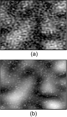
Figure 1: Speckled speckle.  (a) Scalar field  (single polarization component) intensity.  (b) Vector field (two polarization component) intensity. The computer simulated source distributions that produce these calculated speckle patterns consist of two concentric disks of light that illuminate a random phase plate (diffuser). The diameters of these disks differ by a factor of ten, and the total optical power in the smaller disk is ten times the power in the larger disk.  For the scalar field in (a) the illuminating disks have the same linear polarizations, for the vector field in (b) the polarizations are orthogonal.  Individually, the small (large) diameter disk produces large (small) speckle spots. Collectively, in (a) interference between the speckle fields generated by the small and large disks produces the fine granulation of the large speckle spots, whereas the pattern in (b) is the sum of the speckle intensities generated by each disk because orthogonal polarizations do not interfere.  This absence of interference notwithstanding, as discussed in Section III, the polarization singularity structure of the vector field in (b) differs fundamentally from the corresponding singularity structure produced by each disk acting alone.

II SOURCES AND AUTOCORRELATION FUNCTIONS

We assume the (standard two dimensional) geometry shown in Fig. 2, further assume circular Gaussian statistics [$1$] for the two dimensional, paraxial, complex optical field $E\left(x,y\right)$ and its derivatives, and write $E\left(x,y\right)$ in terms of its real $\mathcal{R}\left(x,y\right)$ and imaginary $\mathcal{I}\left(x,y\right)$ parts as

$$E\left(x,y\right)=\mathcal{R}\left(x,y\right)+\text{i}\mathcal{I}\left(x,y\right).$$ (1)

Invoking stationarity and circular symmetry, the normalized autocorrelation function of the field in the plane of observation (the $xy$-plane) is defined by

$$W\left(v\right)=\left\langle E^{\ast}\left(0\right)E\left(v\right)\right\rangle/\left\langle\left|E\right|^{2}\right\rangle,$$ (2)

where $\left\langle...\right\rangle$ represents an ensemble average, and

$$v=\left(x^{2}+y^{2}\right)^{1/2}.$$ (3)

With these assumptions all one and two point statistical properties can be obtained from $W\left(v\right)$ and its derivatives.

We take $E$ to be in the far field of a circularly symmetric planar source $S\left(u\right)$, where $u$ measures radial position in the source plane.  The VanCittert-Zenike theorem [$1$] relates $W\left(v\right)$ and $S\left(u\right)$ by

$$W\left(\kappa v\right)=\int_{0}^{\infty}uS\left(u\right)J_{0}\left(\kappa uv\right)du\,{\large/}\int_{0}^{\infty}uS\left(u\right)du,$$ (4)

where $\kappa=2\pi/\left(\lambda Z\right)$, with $\lambda$ the wavelength of light, and $Z$ the distance to the remote screen on which $E$ is measured.  Here and throughout $J_{n}$ is the Bessel function of integer order $n$.  We define

$$r=\kappa v,$$ (5)

and hereafter write $W\left(\kappa v\right)=W\left(r\right)$.

$S\left(u\right)$ is the intensity distribution (modulus squared) of the field leaving the surface of the random medium (sample).  We assume this sample to be a random phase plate (diffuser) that is deep enough to yield Gaussian statistics, but is not so deep as to produce multiple scattering [$1$]; based on this assumption we equate $S\left(u\right)$ with the intensity distribution illuminating the sample, and assume that the scattered field retains the state of polarization of the incident field.

II.1 Simple sources

We consider initially three different, widely studied simple source distributions that individually generate normal speckle patterns: a Gaussian (superscript G); a disk (superscript D); and a narrow annulus, or ring, (superscript R); writing:

$$S^{\left(\text{G}\right)}\left(u\right) =exp\left[-u^{2}/\left(4p^{2}\right)\right];$$ (6a)

$$S^{\left(\text{D}\right)}\left(u\right) =\Theta\left(u-p\right);$$ (6b)

$$S^{\left(\text{R}\right)}\left(u\right) =\varepsilon\delta\left(u-p\right),$$ (6c)

where $$\varepsilon \Theta\left(w\right) \Theta\left(w\leq 1\right)=1 \Theta\left(w>1\right)=0 \delta\left(w\right)$$ in Eq. (6c) is explained below. Here and throughout is the Heaviside step function defined by , , and is the Dirac Delta function.

Although there are no particular problems in generating experimentally the simple Gaussian and disk source distributions, the ring can only be approximated.  This can be done by using a narrow, but finite width, annulus.  Writing $\mathbb{S}^{\left(\text{R}\right)}\left(u\right)$ for this annulus we have

$$\mathbb{S}^{\left(\text{R}\right)}\left(u\right)=\Theta\left(u-p-\varepsilon/2\right)-\Theta\left(u-p+\varepsilon/2\right),$$ (7)

where $p$ is the mean radius, and $\varepsilon$ the width, of the annulus.  Upon passing to the limit of zero width while noting that

$$\lim_{\varepsilon\rightarrow 0}\left[\mathbb{S}^{\left(\text{R}\right)}\left(u\right)\right]/\varepsilon=\delta\left(u-p\right),$$ (8)

it becomes evident that for consistency with the dimensionless Gaussian and disk source functions, the source function of the ring must be written as in Eq. (6c).

Using Eq. (4) the autocorrelation functions $W$ of the simple sources in Eqs. (6a)-(6c) are

$$W^{\left(\text{G}\right)}\left(pr\right) =exp\left(-p^{2}r^{2}\right),$$ (9a)

$$W^{\left(\text{D}\right)}\left(pr\right) =2J_{1}\left(pr\right)/\left(pr\right),$$ (9b)

$$W^{\left(\text{R}\right)}\left(pr\right) =J_{0}\left(pr\right),$$ (9c)

whereas the autocorrelation function of the finite width annulus, Eq. (7), is [$$3$$]

$$\mathbb{W}^{\left(\text{R}\right)}\left(pr\right) =\frac{1}{p\varepsilon r}[\left(p+\varepsilon/2\right)J_{1}\left(pr+\varepsilon r/2\right)$$

$$-\left(p-\varepsilon/2\right)J_{1}\left(pr-\varepsilon r/2\right)],$$ (10a)

$$\approx J_{0}\left(pr\right)\left[1-\frac{1}{6}\left(\frac{\varepsilon r}{2}\right)^{2}\right]$$

$$-\frac{\varepsilon^{2}r}{24p}J_{1}\left(pr\right)+\mathcal{O}\left(\left(\frac{\varepsilon}{2p}\right)^{4}\right).$$ (10b)

As discussed in [$$3 \varepsilon r\lesssim 1$$], Eq. (10a) is an excellent approximation to Eq. (9c) for , so that experiments with narrow annuli can be expected to closely match the theoretical results obtained here for a delta function ring.

The inverse of the parameter $p$ is a characteristic length that determines many properties of the speckle field.  For example, in all cases the number density of extrema, singularities, umbilic points, etc. equals $cp^{2}/\pi$, where the constant $c$, which does not differ very markedly from unity, depends upon the the form of the autocorrelation function and the nature of the critical point.  Thus, the mean separation between critical points is of order $1/p$, the density of level crossings (line length/unit area) is proportional to $p$, and the mean spacing between crossings along a straight line is proportional $1/p$.

II.2 Composite sources

These important preliminaries completed, we now turn to composite source functions that generate speckled speckle fields.  We build these composite sources out of pairwise combinations of simple Gaussian, disk, and ring sources.  One member of the pair, for which we set $p=a$, has a narrow, but intense, distribution of intensity, the other member, for which we set $p=b$, has a broad but weak intensity distribution.

As a specific example we consider a composite source made up out of two Gaussians.  We generate this source (conceptually) using a single laser beam and an optical system that produces two concentric foci at the diffuser - an intense tight focus, the $a$ beam, and a weak broad focus, the $b$ beam.  The resulting setup is shown schematically in Fig. 2.  Leaving aside the important, practical details of the optical system that produces the $a$ and $b$ beams, we proceed to analyze the properties of the resultant speckled speckle fields.

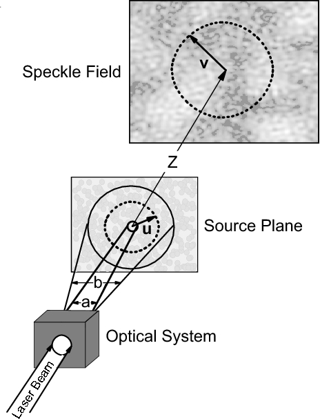
Figure 2: Apparatus for generating speckled speckle.  A laser beam enters an optical system that produces two concentric beams which illuminate a deep phase plate (the source plane).  One beam, labelled $a$, has a small diameter and a large intensity, the other, labelled $b$, has a large diameter and a small intensity.  The resulting speckle field is observed in the far field of the source plane.  Under the paraxial assumption used here, the distance $Z$ between the source plane and speckle field satisfies $Z\gg u,v$.  The orthogonal $xy$ axis system in the speckle field can have an arbitrary orientation, and is not shown.  The large spots in the speckle field are due to beam $a$, the small spots to beam $b$.  For scalar speckled speckle both beams have the same polarization, for vector speckle speckle they are orthogonally polarized.  Using the above geometry, we later illustrate many of the special properties of speckled speckle with a computer simulation in which a source that consists of $1000$ randomly phased points (the Source Plane) with a desired composite amplitude distribution (binary combinations of Gaussians, Disks, and Rings) radiates into the far field (the Speckle Field).

We start by noting that now there are two different characteristic lengths, $\Lambda_{a}=1/a$, and $\Lambda_{b}=1/b$, with $\Lambda_{a}\gg\Lambda_{b}$.  In Fig. 1 it is the $a$ field that generates the large speckle spots, whereas the $b$ field generates the small spots that decorate the $a$ field spots.  Although this result is, obvious, as becomes apparent there are a host of nonobvious, often surprising, phenomena that lie hidden in these patterns

Using superscripts T_a and T_b to denote the source type, where T${}_{a},$T${}_{b}\$= G, D, or R, we write our composite source as

$$S^{\left(\text{T}_{a}\text{T}_{b}\right)}\left(u\right)=I_{a}S^{\text{T}_{a}}\left(u\right)+I_{b}S^{\text{T}_{\text{b}}}\left(u\right),$$ (11)

where $I$ is the illuminating intensity (optical power/unit area): for a Gaussian $I$ is the peak intensity at the center of the Gaussian; for a disk $I$ is the uniform intensity throughout the disk; and for a ring $I$ is the uniform intensity within the annulus.  Inserting Eq. (11) into Eq. (4) we obtain for the autocorrelation function of the composite source

$$W^{\left(\text{T}_{a}\text{T}_{b}\right)}\left(r\right)=\frac{W^{\left(\text{T}_{a}\right)}\left(ar\right)+K^{\left(\text{T}_{a}\text{T}_{b}\right)}W^{\left(\text{T}_{b}\right)}\left(br\right)}{1+K^{\left(\text{T}_{a}\text{T}_{b}\right)}}.$$ (12)

The dimensionless parameter $K^{\left(\text{T}_{a}\text{T}_{b}\right)}$ in Eq. (12) depends on the combination of sources that are used, and is given in Appendix A.  As discussed in this appendix, $K$ equals the total optical power in the $b$ source beam divided by the total optical power in the $a$ source beam, so that the composite field autocorrelation function is the optical power weighted average of the individual $a$ and $b$ autocorrelation functions.

In addition to $W$, we will need throughout later sections mean square derivatives $r_{2n}$ of the real (imaginary) parts of the composite optical field, and moments $M_{2n}$ of the composite source functions, in both cases for $n=1,2,3$; $r_{2n}$ is given in Appendix B, $M_{2n}$ in Appendix C.  We will also need the dimensionless parameter $\eta=r_{4}/r_{2}^{2}-1$, which is discussed in Appendix D.

III CRITICAL POINTS OF THE PHASE

III.1 Scalar Field Statistics and Morphology

III.1.1 Statistics of vortices and phase extrema

General results.

The number density $V$ of vortices [$4-6$], $E$ of phase extrema [$7$], and $S$ of phase saddles, in normal speckle is extended by inspection to speckled speckle as

$$V^{\left(\text{T}_{a}\text{T}_{b}\right)} =r_{2}^{\left(\text{T}_{a}\text{T}_{b}\right)}/\left(2\pi\right),$$ (13a)

$$E^{\left(\text{T}_{a}\text{T}_{b}\right)} =\frac{\left(M_{4}^{{}^{\left(\text{T}_{a}\text{T}_{b}\right)}}\right)^{3/2}}{4\pi M_{2}^{{}^{\left(\text{T}_{a}\text{T}_{b}\right)}}\left(3M_{4}^{{}^{\left(\text{T}_{a}\text{T}_{b}\right)}}-2\left(M_{2}^{{}^{\left(\text{T}_{a}\text{T}_{b}\right)}}\right)^{2}\right)^{1/2}}$$

$$-M_{2}^{{}^{\left(\text{T}_{a}\text{T}_{b}\right)}}/\left(4\pi\right),$$ (13b)

where $$r_{2}^{\left(\text{T}_{a}\text{T}_{b}\right)} M_{2}^{{}^{\left(\text{T}_{a}\text{T}_{b}\right)}} M_{4}^{{}^{\left(\text{T}_{a}\text{T}_{b}\right)}} +1$$ is given in Appendix B, and in Appendix C.  From the requirement that the net Poincaré index of all critical points in the plane equals follows that the densities of vortices, exrema, and saddles, are related by

$$S=V+E.$$ (14)

Statistics for single sources.

$V$ and $E$ for a single source, Eqs. (6a), (6b), and (6c), are recovered from Eqs. (13a) and (13b) by setting $K=0$, with results [$7$]:

$$V^{\left(\text{G}\right)} =\frac{p^{2}}{\pi},\;\;E^{\left(\text{G}\right)}=\frac{p^{2}}{\pi}\left[\sqrt{2}-1\right],$$ (15a)

$$V^{\left(\text{D}\right)} =\frac{p^{2}}{8\pi},\;\;E^{\left(\text{D}\right)}=\frac{p^{2}}{8\pi}\left[2\left(\frac{2}{3}\right)^{\left(3/2\right)}-1\right],$$ (15b)

$$V^{\left(\text{R}\right)} =p^{2}/\left(4\pi\right),\;\;E^{\left(\text{R}\right)}=0.$$ (15c)

For a single source we therefore have $$\left(E/V\right)^{\left(\text{G}\right)}=0.414 \left(E/V\right)^{\left(\text{D}\right)}=0.0887 \left(E/V\right)^{\left(\text{R}\right)}=0 E/V$$, , , so that is always less than unity; for speckled speckle, however, the situation is remarkably different.

Anomalous statistics for compound sources.

In what follows we always take $a<b$, and assume that $\rho=a/b$ is small: only in this limit are there two widely different length scales in the speckle pattern.  We then find that for any given small value of $\rho$ the ratio of phase extrema to vortices, $\left(E/V\right)^{\left(\text{T}_{a}\text{T}_{b}\right)}\equiv E^{\left(\text{T}_{a}\text{T}_{b}\right)}/V^{\left(\text{T}_{a}\text{T}_{b}\right)}$, attains a large, maximum value, $\left(E/V\right)_{max}^{\left(\text{T}_{a}\text{T}_{b}\right)}$, when $K^{\left(\text{T}_{a}\text{T}_{b}\right)}=K_{max}^{\left(\text{T}_{a}\text{T}_{b}\right)}$,where

$$K_{max}^{\left(\text{T}_{a}\text{T}_{b}\right)} =\frac{m_{2}^{\left(\text{T}_{a}\right)}}{m_{2}^{\left(\text{T}_{b}\right)}}\rho^{2},$$

$$\left(E/V\right)_{max}^{\left(\text{T}_{a}\text{T}_{b}\right)} =\frac{\sqrt{3}m_{4}^{\left(\text{T}_{b}\right)}}{12m_{2}^{\left(\text{T}_{a}\right)}m_{2}^{\left(\text{T}_{b}\right)}}\left(\frac{1}{\rho^{2}}\right),$$ (16)

with $m_{2n}^{\left(\text{T}\right)}$ given in Eqs. (70) and (64) .  For example, for $a$ a Gaussian (G) and $b$ a ring (R),

$$K_{max}^{\left(\text{GR}\right)} =\frac{m_{2}^{\left(\text{G}\right)}}{m_{2}^{\left(\text{R}\right)}}\rho^{2}=4\rho^{2},$$ (17a)

$$\left(E/V\right)_{max}^{\left(\text{GR}\right)} =\frac{\sqrt{3}m_{4}^{\left(\text{R}\right)}}{12m_{2}^{\left(\text{G}\right)}m_{2}^{\left(\text{R}\right)}}\left(\frac{1}{\rho^{2}}\right)=\frac{\sqrt{3}}{48\rho^{2}}.$$ (17b)

Comparison of results for single and compound sources.

We compare the above results for speckled speckle with those for ordinary speckle.  For, say, $\rho=0.1$, which should be achievable in practice without undue difficulty, we have: for two Gaussians, $\left(E/V\right)_{max}^{\left(\text{GG}\right)}\approx 29$, which is $70$ times larger than for normal speckle, Eq. (15a); for two disks$\;\left(E/V\right)_{max}^{\left(\text{DD}\right)}\approx 19$, which is $215$ larger than for normal speckle, Eq. (15b); and for two rings $\left(E/V\right)_{max}^{\left(\text{RR}\right)}\approx 14$.  This latter result is especially striking when it is recalled that for normal speckle, Eq. (15c), there are no phase exrema at all.  We note that in all three of the above cases $K_{max}=0.01$, which corresponds to an intensity ratio $I_{b}/I_{a}=10^{-4}$ and a total optical power ratio $P_{b}/P_{a}=0.01$.  It thus seems likely that the major experimental problem in observing the anomalies of speckled speckle will be the reduction of parasitic light that would tend to swamp the weak $b$ field intensity $I_{b}$.

Representative Graphs.

In Fig. 3 we display graphs of $V$, $E$, and $E/V$, for two Gaussians (GG), two disks (DD), and two rings (RR).  The graphs for say DR ($a$ = D, $b$ = R) or RD ($a$ = R, $b$ = D) can be approximated by dividing the figures along the line $K=10^{-2}$ and connecting the appropriate combination of vertically rescaled figure halves; for example, the figure for DR is approximated by attaching the left half of Fig. 3(b) to the right half of Fig. 3(c).

Figure 3: Critical point densities, $V$, $E$, and $E/V$, vs. $K$ for $a=1,b=10$ ($\rho=0.1$), for (a) two Gaussians (GG), (b) two disks (DD), and (c) two rings (RR).  Note the logarithmic scales.

The graphs in Fig. 3 are representative, and other source combinations show similar results: the density of vortices ($V$), Eq. (13a), interpolates smoothly from its $a$ value (small $K$) to its $b$ value (large $K$), as does the density (not shown) of saddle points, Eq. (14), whereas both the density of extrema ($E)$, Eq. (13b), and the ratio $E/V$, are anomalous, and reach a maximum for small $K$.  The density of these maxima can be made arbitrarily large by suitable choice of $\rho$ and $K$, Eq. (16).

III.1.2 Morphology

Spatial arrangements of vortices.

The spatial arrangement of the vortices is also anomalous.  Because a vortex is an absolute zero of the wavefunction [$8$], vortices can appear only where there is complete destructive interference between the strong $a$ and weak $b$ fields, so composite field vortices are constrained to lie in simultaneously dark regions of the $a$ field, and the composite field, speckle patterns, Fig. 4.  For very small $I_{b}/I_{a}$ the $b$ field is a minor perturbation of the $a$ field. In this limit the sparse zeros, and therefore the sparse vortices, of the $a$ field maintain their identities but are shifted slightly in position, Fig. 4(a). For larger intensity ratios, however, both $a$ and $b$ field vortices lose their identities.

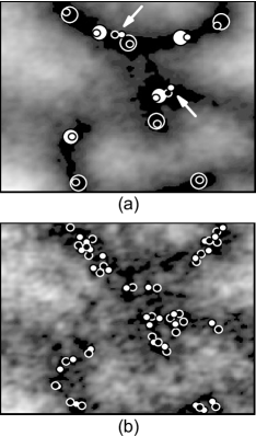
Figure 4: Speckled speckle phase vortices for Gaussian $a$ and $b$ fields (GG) with $\rho=a/b=0.1$.  Shown is a typical region of the intensity speckle pattern with vortices superimposed, where filled white circles with black rims (filled black circles with white rims) represent positive (negative) vortices.  (a) $I_{b}/I_{a}=2\times 10^{-5}$ ($K=0.002$).  The large circles show the positions of the vortices of the strong $a$ field ($I_{b}=0$), the small circles show the vortices of the composite field.  As expected, for the small $I_{b}/I_{a}$ ratio used here, the composite field vortices cluster near the positions of the sparse $a$ field vortices, which are the darkest regions of the speckle pattern.  As $I_{b}/I_{a}$ is increased from zero, and as is illustrated here, initially the $a$ field vortices undergo small displacements but maintain their identities, while a small number of new positive/negative vortex pairs nucleate (here two pairs, arrows).  (b)  The field in (a) for $I_{b}/I_{a}=10^{-3}$ ($K=0.1$).  As $I_{b}/I_{a}$ increases the number of composite field vortices increases rapidly (Fig. 3), and in addition to vortex nucleation vortex annihilation also occurs, leading to a loss of identity of the $a$ field vortices.  For the moderately small $I_{b}/I_{a}$ ratio used here the composite field vortices no longer need cluster around the positions of the $a$ field vortices; they are, however, still constrained, to lie in the dark regions surrounding the large $a$ field speckle spots.  For still larger $K$ vortices begin to fill the field more uniformly, and in the limit of large $K$ the dense vortex structure is that of the $b$ field.

Reactions between vortices and phase stationary points.

As $I_{b}$ increases new vortices appear.  Conservation of charge requires these vortices to nucleate as positive/negative pairs.  Pair production by itself, however, violates conservation of the Poincaré index, here $I_{P}$, because $I_{P}=+1$ for vortices independent of their charge.  Vortex pair production must therefore be accompanied by another process, and in general there are two possibilities:

I. A vortex pair and a pair of saddle points (each one of which has $I_{P}=-1)$ are generated [$9$].

II. Two extrema (one minimum and one maximum, each of which has $I_{P}=+1$) collide and annihilate, and a vortex pair emerges from the collision [$10$].

For very small $I_{b}$ there are, in general, fewer extrema than vortices, so in this regime mechanism II cannot be operative (recall that for a ring there are no phase extrema at all), leaving mechanism I as the only alternative.  In Fig. 3 this regime corresponds to the region of say $K<10^{-4}$.  But as can be seen from this figure, for larger $K$ the number of extrema exceeds the number of vortices, thereby permitting mechanism II to become operative.  These two reaction mechanisms are illustrated in Fig. 5 for the representative case of GG for small and intermediate $K$, and in Fig. 6 for RR for larger $K$; as can be seen from these figures, for sufficiently small (large) $K$ mechanism I (mechanism II) dominates.

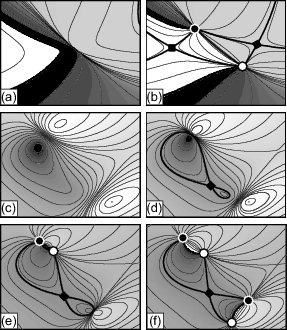
Figure 5: Phase maps showing vortex nucleation for small and intermediate $K$ for Gaussian $a$ and $b$ source fields (GG) with $a/b=0.1$.  The phase increases $0$ to $2\pi$ black to white.  Filled black (white) circles represent negative (positive) vortices, whereas black squares mark saddle points.  Thin curves are ordinary contours, thick curves are the special contours (bifurcation lines) that pass through the saddle points.  (a),(b) Vortex nucleation for very small $K$.  (a)  $K=0.00164$.  (b) $K=0.0017$.  In this small $K$ region mechanism I of the text is dominant, and vortex pairs nucleate together with a pair of saddle points.  The resulting box like structure, first described in [$9$], is the one usually observed following vortex pair production in normal speckle.  (c)-(f) Intermediate $K$ regime.  In (c), (d), (e), and (f), $K=0.024,0.0275,0.0291,$ and $0.0325$, respectively.  In this region mechanism II of the text dominates.  Specifically: in (c) there are no vortices, only phase extrema (two maxima and one minimum); in (d) the upper minimum and maximum approach one another, while in an unrelated process a new saddle point and a new minimum nucleate; in (e) the upper pair of extrema collide and generate a positive/negative vortex pair; and in (f) the lower pair of extrema collide and generate a second vortex pair.

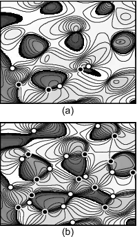
Figure 6: Phase maps showing vortex nucleation for larger values of $K$ for both $a$ and $b$ source fields rings (RR) with $a/b=0.1$.  Symbols are as in Fig. 5.  (a) $K=0.5$.  (b) $K=2$.  In (a), which corresponds approximately to the region of the flat maximum in the number of extrema E in Fig. 3c, there are three vortex pairs and numerous maxima and minima.  In (b), which corresponds to the onset of rapid decline in the number of extrema in Fig. 3c, all maxima and minima in (a) have collided, annihilated, and been replaced by vortex pairs.  

III.2 Vector Field C points and Extrema

III.2.1 Introductory remarks

The state of polarization of generic vector fields is elliptical. In the paraxial fields of interest here the (always planar [$11$]) polarization ellipses lie in planes, here the $xy$-plane, oriented normal to the direction of propagation, the $Z$-axis.  The point singularities of such fields in the plane (in space) are C points (form continuous C lines), which are points (lines) of circular polarization embedded in a field of elliptical polarization [$12$].  Because the azimuthal orientation of a circle (the C circle) is undefined, the surrounding ellipses rotate about the point, generically with rotation (winding) angle $\pm\pi$, and topological charge (winding number) $\pm\frac{1}{2}$ for positive/negative points [$12$].

Necessarily associated with C points in the planes of generic paraxial fields are azimuthal stationary points - extrema (maxima and minima$|$), and saddle points [$13$].  Unlike C points which are easily identified visually as the centers around which the surrounding ellipses rotate, azimuthal stationary points are subtle features that may be difficult to discern in traditional maps that show polarization ellipses.  A highly useful representation that shows both types of critical points clearly is the phase (argument) $\Phi_{12}$ of the complex Stokes field [$14$]

$$S_{12}=S_{1}+i\,S_{2}$$ (18)

In this representation C points are vortices with charges $\pm 1$, and azimuthal stationary points are phase maxima, minima, and saddle points.  In what follows we use this representation exclusively.

Charge conservation requires that C points nucleate or annihilate as positive/negative pairs, whereas conservation of the Poincaré index $I_{P}$, which is $+1$ for C points of either sign, requires that pair production be accompanied by either the production of two azimuthal saddles, for which $I_{P}=-1$, or the disappearance of two extrema, for which $I_{P}=+1$.

Like ordinary circularly polarized light, C points are either right handed or left handed, depending upon the direction of rotation (clockwise or counterclockwise) of the electric vector of the light as it traces out the C circle.  By continuity, the polarization ellipses in the immediate vicinity of a C point have the handedness of the point, so that overall the ellipse field is divided into right and left handed regions.  Near the boundary between regions of opposite handedness the polarization ellipses narrow, and on the boundary itself the ellipses collapse into lines and the polarization is linear; these lines are called L lines [$12$].

All of the above holds for both ordinary, and speckled speckle, vector fields.

We now turn to a discussion of the number densities of C points and their associated extrema in vector speckled speckle.  Here the $a$ and $b$ source fields have orthogonal polarizations, and we consider two different cases: in the first the $a$ ($b$) source field is linearly polarized along the $x$-axis ($y$-axis); in the second the $a$ ($b$) source field has right (left) circular polarization.  As becomes apparent, these two different configurations produce very different results.

III.2.2 Linearly polarized source fields: statistics and ellipse field morphology

a.  C point densities.

In what follows we assume, as already stated, that speckle field $E_{x}$ ($E_{y}$) maintains the state of linear polarization of its $a$ ($b$) source. We begin by noting that at a C point the amplitudes of $E_{x}$ and $E_{y}$ must be equal, so like phase vortices, C points of the composite field are found in the dark regions of the $a$ field speckle pattern [$2$].  But unlike vortices, these regions need not also be dark regions of the composite field speckle pattern, because unlike a vortex, a C point is not a zero of the vector field.

In considering number densities it is convenient to decompose the speckle field, Fig. 2, into right (R) and left (L) circularly polarized components, $E_{R}$ and$\ E_{L}$.  The reason is that $E_{R}$ ($E_{L}$) vanishes at a right handed (left handed) C point, and since the single polarization component fields $E_{R}$ and $E_{L}$ are scalar fields, Eq. (13a) is applicable to each component.  From this follows that in normal speckle fields the number density of C points is twice the density of phase vortices [$12$].

Eq. (13a) is also applicable to C points in vector speckled speckle, but to use this result we need derivatives $r_{2}^{\left(\text{T}_{a}\text{T}_{b}\right)}$ for the circularly polarized components.  Using the results in Appendix B, we can obtain these derivatives from the autocorrelation functions $W_{R,L}^{\left(\text{T}_{a}\text{T}_{b}\right)}$ of $E_{R}$ and$\ E_{L}$; these autocorrelation functions are calculated below.

We start by writing the circularly polarized components $E_{R}$  and $E_{L}$ in terms of the Cartesian components $E_{x}$ and $E_{y}$ of the speckle field as

$$E_{R,L}=\left(E_{x}\mp iE_{y}\right)/\sqrt{2},$$ (19)

where $E_{x}$ ($E_{y}$) arises from the $x$-axis ($y$-axis) linearly polarized $a$ ($b$) source field.  Temporarily suppressing for notational convenience superscripts T_aT_b, $W_{R,L}$ is

$$W_{R,L}\left(r\right)=\left\langle E_{R,L}^{\ast}\left(0\right)E_{R,L}\left(r\right)\right\rangle/\left\langle I_{R,L}\right\rangle$$ (20)

where the average intensity $\left\langle I_{R,L}\right\rangle=\left\langle E_{R,L}^{\ast}\left(0\right)E_{R,L}\left(0\right)\right\rangle=\tfrac{1}{2}\left(\left\langle I_{x}\right\rangle+\left\langle I_{y}\right\rangle\right)$, with $\left\langle I_{x}\right\rangle$ and $\left\langle I_{y}\right\rangle$ the average intensities of the Cartesian components.  Using Eq. (19) together with $\left\langle E_{x}^{\ast}\left(0\right)E_{y}\left(r\right)\right\rangle=\left\langle E_{y}^{\ast}\left(0\right)E_{x}\left(r\right)\right\rangle=\left\langle E_{x}^{\ast}\left(0\right)E_{y}\left(0\right)\right\rangle=\left\langle E_{y}^{\ast}\left(0\right)E_{x}\left(0\right)\right\rangle=0$, we have

$$W_{R}^{\left(\text{T}_{a}\text{T}_{b}\right)}\left(r\right)=W_{L}^{\left(\text{T}_{a}\text{T}_{b}\right)}\left(r\right)=W^{\left(\text{T}_{a}\text{T}_{b}\right)}\left(r\right),$$ (21)

where $W^{\left(\text{T}_{a}\text{T}_{b}\right)}\left(r\right)$ is given in Eq. (12), and $K$ is given in Eq. (58).  In obtaining this result we use the fact that$\ \left\langle I_{x}\right\rangle$ ($\left\langle I_{y}\right\rangle$) is proportional to the total optical power in the source field $a$ ($b$) component, so that $\left\langle I_{y}\right\rangle/\left\langle I_{x}\right\rangle=K$.  Thus, Eq. (13a) and curves $V$ in Fig. 3, multiplied by a factor of two, also describe C points in vector speckled speckle.

b.  L line densities.

The density (line length/unit area) of L lines is proportional to the square root of the density of C points [$15$].  Because the density of C points, $2V$, interpolates smoothly between its small $K$ ($a$ field) and large $K$ ($b$ field) limits, so does the L line density, and L lines in speckled speckle do not show anomalies.

c.  Densities of azimuthal extrema.

K and $\rho=a/b$ both small.

Although Eq. (13a) is applicable to speckled speckle C points, Eq. (13b) is not necessarily applicable to the corresponding azimuthal stationary points; the reason is that unlike the case of C points, there is no a priori simple relationship between vector field azimuthal stationary points and the stationary points of the corresponding scalar field components.  At present there is no exact theory for the azimuthal densities; we are, however, able to estimate these densities when both $K$ and $a/b$ are small.

Returning to Eq. (19) we write

$$\sqrt{2}E_{R,L}=E_{x}\left(1\mp iE_{y}/E_{x}\right),$$ (22)

where the motivation for this form is the fact that when $K$ is small so also is $E_{y}/E_{x}$.  Writing the various field components in terms of amplitudes $A$ and phases $\varphi$ or $\Phi$,

$$E_{x} =A_{x}\exp\left(i\varphi_{x}\right),$$ (23a)

$$E_{y} =A_{y}\exp\left(i\varphi_{y}\right),$$ (23b)

$$E_{R} =A_{R}\exp\left(i\Phi_{R}\right),$$ (23c)

$$E_{L} =A_{L}\exp\left(i\Phi_{L}\right),$$ (23d)

and noting that Stokes parameters $$S_{1} S_{2}$$ and can be written

$$S_{1} =2\operatorname{Re}\left(E_{R}^{\ast}E_{L}\right),$$ (24a)

$$S_{2} =2\operatorname{Im}\left(E_{R}^{\ast}E_{L}\right),$$ (24b)

we have from Eq. (18)

$$S_{12}=2E_{R}^{\ast}E_{L},$$ (25)

from which follows

$$\Phi_{12}=\Phi_{L}-\Phi_{R}.$$ (26)

Returning to Eq. (22) we have to third order in the small quantity $E_{y}/E_{x}$,

$$1\pm iE_{y}/E_{x} \approx\exp\left((E_{y}/E_{x})^{2}/2\right)$$

$$\times\exp\left(\mp\text{i\thinspace}\left(E_{y}/E_{x}-\left(E_{y}/E_{x}\right)^{3}/3\right)\right).$$ (27)

Writing

$$E_{y}/E_{x}=\left(A_{y}/A_{x}\right)\left[\cos\left(\varphi_{y}-\varphi_{x}\right)+\text{i\thinspace}\cos\left(\varphi_{y}-\varphi_{x}\right)\right],$$ (28)

we have

$$\Phi_{R,L} =\varphi_{x}\mp\left(A_{y}/A_{x}\right)\cos\left(\varphi_{y}-\varphi_{x}\right)$$

$$+\tfrac{1}{2}(A_{y}/A_{x})^{2}\sin\left(2\left(\varphi_{y}-\varphi_{x}\right)\right)$$

$$\pm\tfrac{1}{3}(A_{y}/A_{x})^{3}\cos^{3}\left(\varphi_{y}-\varphi_{x}\right)$$

$$\mp(A_{y}/A_{x})^{3}\sin\left(\varphi_{y}-\varphi_{x}\right)\sin\left(2\left(\varphi_{y}-\varphi_{x}\right)\right).$$ (29)

so that to leading order in $A_{y}/A_{x}$,

$$\Phi_{12} \approx-2\left(A_{y}/A_{x}\right)\cos\left(\varphi_{y}-\varphi_{x}\right)$$ (30a)

$$\approx 2\left(\Phi_{L}-\varphi_{x}\right)$$ (30b)

$$\approx-2\left(\Phi_{R}-\varphi_{x}\right).$$ (30c)

Eqs. (30) make a number of possibly unexpected predictions that are listed below.

Density of azimuthal extrema for $K$ equal to its value at the peak of curve E in Fig. 3.

Far from its sparse vortices the phase $\varphi_{x}$ of the slowly varying $a$ field changes slowly, so that in regions where $\Phi_{R,L}$ vary rapidly, $\varphi_{x}$ in Eqs. (30b) and (30c) can be treated locally as an unimportant, nearly flat background that can be eliminated by a local redefinition of the zero of phase.  For sufficiently small $\rho=a/b$ these flat regions occupy most of the wavefield area and we can write

$$\Phi_{12}\approx 2\Phi_{L}\approx-2\Phi_{R}.$$ (31)

In the region of the peak of curve E in Fig. 3, where there is a high density of extrema, $\Phi_{R,L}$ vary rapidly.  We therefore conclude that near this peak the density of azimuthal extrema very nearly equals the density of phase extrema $E$, so that just like for scalar speckle speckle, $E/V$ for vector speckle speckle can attain very large values.

In Fig. 7 we compare $\varphi_{x}$, $\Phi_{12}$, $\Phi_{L}$, and $-\Phi_{R}$ for the case of two disks (DD) for the small, but still experimentally possible, ratio $a/b=0.01$, for $K=1\times 10^{-4}$, which corresponds to the maximum of $E/V$ for the above $a/b$ ratio (here $\left(E/V\right)_{\max}=1924$).  These parameters are favorable ones, and for larger $a/b$ ratios, say $a/b=0.1$, the very close agreement with the predictions of Eqs. (31) degrades, because now $\varphi_{x}$ can no longer be considered to be locally flat over most of the wavefield area; the overall conclusion, however, remains, and in general $E/V$ is anomalously large for vector speckle speckle.

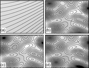
Figure 7: Azimuthal extrema in vector speckled speckle for $a/b=0.01$, and $K=10^{-4}$.  The amplitude in these contour maps increases black to white, so that high maxima (deep minima) are colored white (black).  (a) $\varphi_{x}$. The variation in $\varphi_{x}$ is less than $7\%$ of the variation of $\Phi_{12}$ over this same region, so to first order $\varphi_{x}$ can be taken to be constant in Eqs. (30).  (b) $\Phi_{12}$.  (c) $-\Phi_{R}$.  The minus sign turns maxima into minima and vice versa, facilitating comparison with $\Phi_{12}$ and $\Phi_{L}$.  (d) $\Phi_{L}$.  Note the close similarity of the three fields $\Phi_{12}$, $\Phi_{L}$, and $\Phi_{L}$, in full accord with Eqs. (31).

Density of azimuthal extrema for $K$ less than its value at the peak of curve E in Fig. 3.

For small ratios $a/b$ for all values of $K$ less than $K_{0}$, the value of $K$ at the peak of the $E$ curve, the stationary point structure of $\Phi_{12}$ remains very nearly independent of $K$.  This follows from the fact that not only the phase $\varphi_{x}$ of the slowly varying $a$ field hardly changes, but that also $A_{x}$, the amplitude of the field, changes slowly, and can therefore locally be taken to be constant.  Eliminating $\varphi_{x}$ by redefining the local zero of phase, and replacing $A_{x}$ by a local constant $c$, we have

$$\Phi_{12}\approx-cA_{y}\cos\left(\varphi_{y}\right).$$ (32)

Now, for a given value of $\rho$, the structure of $A_{y}$, and the structure and magnitude of $\varphi_{y}$, are independent of $I_{a}$ and $I_{b}$, and are therefore independent of $K$; Eq. (32) therefore implies that although the magnitude of $\Phi_{12}$ changes with $K$, its structure remains invariant.  This is illustrated qualitatively in Fig. 8(a).

In Fig. 8(b) we quantify the relationship between $\Phi_{12}$ and $\Phi_{L}$.  Shown is the cross correlation coefficient $C$ between $\Phi_{12}\left(K\right)$ and $\Phi_{L}\left(K_{0}\right)$, where $C=C\left(u,v\right)$ for two real variables $u,v$ is

$$C\left(u,v\right)=\frac{\left\langle\left(u-\left\langle u\right\rangle\right)\left(v-\left\langle v\right\rangle\right)\right\rangle}{\sqrt{\left\langle\left(u-\left\langle u\right\rangle\right)^{2}\right\rangle\left\langle\left(v-\left\langle v\right\rangle\right)^{2}\right\rangle}}.$$ (33)

Here $\left\langle...\right\rangle$ represents spatial averages over the phase fields. As can be seen, $\Phi_{12}$ and $\Phi_{L}$ are nearly identical ($C=0.983$) up to and including the point at which $E$ passes through its maximum, showing that in vector speckled speckle the density of azimuthal extrema all throughout the small $K$ region substantially equals the maximum value of $E$ for scalar speckled speckle.

An interesting, possibly counterintuitive, feature of Fig. 8(b) is the significant degree of correlation ($C=0.8$) between $\Phi_{12}$ and $\Phi_{L}$ in the large $K$ region where most extrema have been converted to C points.  This correlation reflects the fact that locally the phase field before and after collisions of extrema maintains more-or-less the same value.  This behavior is most clearly seen in Fig. 6, where dark (light) regions in Fig. 6(a) for the most part remain dark (light) in Fig. 6(b).

Generation of C points as $K$ increases from zero.

As noted above, the density of C points increases with $K$ in accord with curves $V$ (multiplied by two) in Fig. 3.  For scalar speckled speckle vortex generation in the small $K$ region in which extrema are sparse occurs via mechanism I in which a new vortex pair appears together with a pair of saddle points, Figs. 5(a),(b), whereas in the region of larger $K$ in which extrema are plentiful vortex pairs are generated via mechanism II in which the collision and annihilation of a pair of extrema, one maximum and one minimum, generates the vortices, Figs. 5(c)-(f) and Fig. 6.  For C points, however, extrema are abundant for both small and large $K$, and it is mechanism II, i.e. collision of azimuthal extrema, that dominates C point production for all $K$.

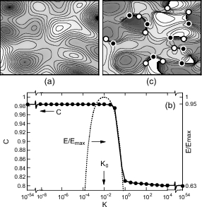
Figure 8: Azimuthal extrema for two disks (DD) for $a/b=0.01$, as in Fig. 7. (a) $\Phi_{12}$ for $K=10^{-54}$.  Note that the stationary point structure here is very nearly the same as in Fig. 7(b) where $K=10^{-4}$ is fifty orders of magnitude larger.  (b) Correlation coefficient $C=C\left(\Phi_{L}\left(K_{0}\right),\Phi_{12}\left(K\right)\right)$, Eq. (33). $\ \Phi_{L}$ is the phase of the left circularly polarized vector field component, $\Phi_{12}$ is the Stokes phase of the combined vector field.  $K_{0}=$ $10^{-2}$ is the value of $K$ at which the scaled number density $E/E_{\max}$ of $\Phi_{L}$ extrema, dotted curve, attains its maximum value. Curve $E/E_{\max}$ is plotted as $1+\log_{10}\left(E/E_{\max}\right)$, so that where $C=0.98$ ($C=0.8$), $E/E_{\max}=$ $0.95$ ($E/E_{\max}=$ $0.63$).  Note the extreme range of $K$, $10^{-54}\leq K\leq$ $10^{54}$.   (c) $\Phi_{12}$ for $K=1$.  As can be seen, when $K$ starts to become large the azimuthal maxima and minima in (a) start to collide and annihilate, generating positive/negative C point pairs (filled white/black circles).  

d.  Decrease in the number of azimuthal extrema for large $K$.

In the limit of large $K$ where $E_{x}/E_{y}$ is small, the analog of Eq. (22) is

$$\sqrt{2}E_{R,L}=\mp\text{i\thinspace}E_{y}\left(1\pm\text{i\thinspace}E_{x}/E_{y}\right),$$ (34)

and the analogs of Eqs. (30) are

$$\Phi_{12} \approx-2\left(A_{x}/A_{y}\right)\cos\left(\varphi_{x}-\varphi_{y}\right)+\pi,$$ (35a)

$$\approx 2\left(\Phi_{L}-\varphi_{y}\right),$$ (35b)

$$\approx-2\left(\Phi_{R}-\varphi_{y}\right).$$ (35c)

For large $$K \Phi_{L} \Phi_{R} \varphi_{y} E K K$$, in scalar fields , , and , decreases from its large maximum to its small single component value (Fig. 3).  Eqs. (35) therefore imply that also the large density of extrema present in vector speckled speckle for small decreases for large .  For scalar fields the reduction in the number of extrema results from collisions of maxima and minima that produce vortex pairs, Figs. 5 and 6; as is illustrated in Fig. 8(c), the same is true for vector speckled speckle.

e. C points for vanishingly small values of either the $a$ or the $b$ field.

As $K$ increases the phase structure stabilizes asymptotically at a mix of C points and extrema, with C points outnumbering extrema by perhaps a factor of $3-5$.  But if for, say, $\left|E_{x}\right|=10^{-25}\left|E_{y}\right|$ ($K=10^{54}$), how, for all intents and purposes, can the wavefield be anything other than linearly polarized?  The answer [$12$, sect. 12.5] is that $E_{y}$ goes continuously to zero at its vortices, so that surrounding each $E_{y}$ vortex, which is an $I_{y}=\left|E_{y}\right|^{2}$ zero minimum, there is for every $K$ an elliptical contour on which $\left|E_{x}\right|=\left|E_{y}\right|$. The size of this contour shrinks with increasing $K$, so for sufficiently large $K$ the phase $\varphi_{x}$ of $E_{x}$ on the contour can be taken to be constant.  Because the phase field surrounding the $E_{y}$ vortex winds through $2\pi$ there are always two points on the contour (separated by $180^{o}$) where $\left|\varphi_{y}-\varphi_{x}\right|=\pi/2$; at these points a positive/negative pair of C points appears.  Similar considerations apply to the limit of very small $K$, where the $C$ points are located near the vortices of $E_{x}$.

f.  Comparison of results for scalar and vector fields.

We conclude this subsection with a summary of the similarities and differences in the number densities of vortices, C points, and extrema, in scalar and in linearly polarized speckled speckle:  (i) For both cases the density of singularities - vortices for the scalar case, C points for the linearly polarized vector case - interpolates smoothly with $K$ from its small $a$ field value to its large $b$ field value: Fig. 3, curve $V$ for vortices; this same curve multiplied by two for C points.  (ii) For the scalar case the density of extrema, and the ratio of extrema to vortices, increase from their $a$ field values to large maxima at small $K$, and then decrease for large $K$ to their $b$ field values: Fig. 3; Eqs. (16).  (iii) For the vector case the density of extrema, and the ratio of extrema to C points, are large for all small $K$, and decrease for large $K$.  For sufficiently small $a/b$ the large azimuthal extrema density for small $K$ substantially equals the maximum density of phase extrema for the scalar case, whereas the large ratio of azimuthal extrema to C points equals half the maximum ratio of phase extrema to vortices for the scalar case.  (iv) In the scalar case generation of vortex pairs is accompanied by nucleation (annihilation) of a pair of saddle points (extrema) for small (large) $K$.  For the vector case C point generation in speckled speckle occurs through the annihilation of paired azimuthal extrema for all $K$.  (v) The reduction in the number of extrema for large $K$ results from collisions of maxima and minima to produce vortices in the scalar case, C points in the vector case.

III.2.3 Circularly polarized source fields

We take the $a$ ($b$) field to be right (left) circularly polarized, and write the circular components in the speckle plane as

$$E_{R} =A_{a}\exp\left(i\varphi_{a}\right),$$ (36a)

$$E_{L} =A_{b}\exp\left(i\varphi_{b}\right).$$ (36b)

Eq. (26) then becomes

$$\Phi_{12}=\varphi_{b}-\varphi_{a},$$ (37)

which implies the following: (i) The number densities, and the spatial distributions of all critical points - C points, azimuthal extrema, and azimuthal saddle points - are independent of $K$, which depends on the amplitudes of the fields, but not on their phases.  (ii) For small values of $a/b$ for which the slowly varying $a$ field phase $\varphi_{a}$ can, over most of the wavefield area, be treated locally as a constant, the critical point structure of $\Phi_{12}$ is essentially the same as that of $\varphi_{b}$.  In this limit the critical point number densities are those of scalar field $b$, and are given by Eqs. (15) with $p=b$.  These conclusions are fully verified by our computer simulations (not shown).  Thus, in contrast to linearly polarized speckled speckle with its rich set of anomalies, circularly polarized speckled speckle appears to offer little that is of special interest.

III.3 Zero Level Crossings of Phase Derivatives

Introductory remarks.

Nodal domains and the zero level curves that define them are of considerable current interest because they determine many important properties of random fields [$1$].  At present there is little information available on the nodal domains of ordinary vector speckle; this prevents us from using our present methods to calculate these domains for vector speckled speckle, and below we consider nodal domains of the phase only of scalar speckled speckle.

Densities of zero crossings and densities of intersections of these crossings with a straight line.

Phase extrema, saddles, and vortices [$16$], are all located at intersections of the zero level crossings Z_x and Z_y of the first order phase derivatives $\varphi_{x}$ and $\varphi_{y}$.  It is therefore reasonable to expect that like the number density of extrema, E, which shows an anomalous peak in Fig. 3 at $K\sim 0.13$, also the line densities $D_{x}=D_{y}=D$ of Z_x and Z_y would show similar anomalous peaks.

For many types of random curves in an isotropic field there is a simple relationship [$15$] between $\mathcal{D}$ and the density $N$ of intersections of these curves with a straight line, say the $x$-axis,

$$\mathcal{D}=\frac{\pi}{2}N.$$ (38)

This relationship, however, does not hold for level curves of derivatives because, as discussed below for the phase, differentiation destroys the required isotropy.

III.3.1 Densities of intersections of zero crossings of phase derivatives with the $x$-axis.

General results.

Previously, we calculated for normal speckle the quantities $N_{x}\left(\varphi_{x},L\right)$ ($N_{x}\left(\varphi_{y},L\right)$), which are the density of intersections of crossings at level $L$ of phase derivatives $\varphi_{x}$ ($\varphi_{y}$) with the $x$-axis [$17$]. Extending by inspection these results to the zero crossings Z_x and Z_y of speckled speckle, we have

$$N_{x,x}^{\left(\text{T}_{a}\text{T}_{b}\right)}=N_{x}^{\left(\text{T}_{a}\text{T}_{b}\right)}\left(\varphi_{x},0\right)=\frac{\sqrt{r_{2}^{\left(\text{T}_{a}\text{T}_{b}\right)}}}{\pi}\left[\eta^{\left(\text{T}_{a}\text{T}_{b}\right)}\right]^{1/2},$$ (39)

where $r_{2}^{\left(\text{T}_{a}\text{T}_{b}\right)}$ is given in Appendix B, $\eta^{\left(\text{T}_{a}\text{T}_{b}\right)}$ in Appendix D.

Now, in the isotropic random field of interest here, on average the length/unit area of Z_x and Z_y must be the same, therefore, if Eq. (38) were to hold we would have $N_{x}^{\left(\text{T}_{a}\text{T}_{b}\right)}\left(\varphi_{x},0\right)=N_{x}^{\left(\text{T}_{a}\text{T}_{b}\right)}\left(\varphi_{y},0\right)$; but this is not the case, and instead [$17$]

$$N_{x,y}^{\left(\text{T}_{a}\text{T}_{b}\right)}=N_{x}^{\left(\text{T}_{a}\text{T}_{b}\right)}\left(\varphi_{y},0\right)=\frac{\sqrt{r_{2}^{\left(\text{T}_{a}\text{T}_{b}\right)}}}{\pi}$$

$$\times E\left(\sqrt{\frac{2-\eta^{\left(\text{T}_{a}\text{T}_{b}\right)}}{3}}\right),\;\eta^{\left(\text{T}_{a}\text{T}_{b}\right)}\leq 2,$$

$$=\frac{\sqrt{r_{2}^{\left(\text{T}_{a}\text{T}_{b}\right)}\left(\eta^{\left(\text{T}_{a}\text{T}_{b}\right)}+1\right)}}{\sqrt{3}\pi}$$

$$\times E\left(\sqrt{\frac{\eta^{\left(\text{T}_{a}\text{T}_{b}\right)}-2}{\eta^{\left(\text{T}_{a}\text{T}_{b}\right)}+1}}\right),\;\eta^{\left(\text{T}_{a}\text{T}_{b}\right)}\geq 2,$$ (40)

where $E$ is the complete elliptic integral of the second kind.

Results for a single source.

Eqs. (39) and (40) with single superscripts hold, of course, for ordinary speckle.  For a Gaussian (G), disk (D), and ring (R), $\eta^{\left(G\right)}=2$, $\eta^{\left(D\right)}=1$, $\eta^{\left(R\right)}=1/2$, and

$$N_{x,x}^{\left(G\right)}/N_{x,y}^{\left(G\right)} =0.900,$$ (41a)

$$N_{x,x}^{\left(D\right)}/N_{x,y}^{\left(D\right)} =0.699,$$ (41b)

$$N_{x,x}^{\left(R\right)}/N_{x,y}^{\left(R\right)} =0.524,$$ (41c)

i.e. $$N_{x,x}^{\left(T\right)}<N_{x,y}^{\left(T\right)}$$ in all three cases.

Anomalous reversals for compound sources.

From Eqs. (39), (40), and (63), it follows that $b^{-1}N_{x,x}$ and $b^{-1}N_{x,y}$ are functions only of $\rho=a/b$ and $K$.  Accordingly, in Fig. 9(a) we plot $b^{-1}N_{x,x}^{\left(\text{DD}\right)}$ and $b^{-1}N_{x,y}^{\left(\text{DD}\right)}$ vs. $K$ for two disks (DD) for $\rho=0.1$.  As can be seen, for very small and very large $K$ (the regions labelled ‘b’ in the figure) $N_{x,x}^{\left(\text{DD}\right)}<N_{x,y}^{\left(\text{DD}\right)}$, in agreement with Eq. (41b).  In the intermediate region $10^{-4}<K<1$ (region ‘c’), however, this situation reverses, and anomalously $N_{x,x}^{\left(\text{DD}\right)}>N_{x,y}^{\left(\text{DD}\right)}$.  This reversal is a general feature, and occurs also for two Gaussians (GG) and two rings (RR), both of which yield graphs that are quite similar to Fig. 9(a).

Explanation of anomalous reversals.

The anomalous $N_{x,x}/N_{x,y}$ ratio, as well as the normal ratio, find their explanation in the structure of the phase field.  For normal speckle, and in regions ‘b’ of Fig. 9(a) for speckled speckle, vortices outnumber extrema.  As discussed in [$16$], in the immediate vicinity of a vortex Z_x (Z_y) is necessarily strictly parallel to the $x$-axis ($y$-axis), Fig. 9(b).  As a result the number of Z_x (Z_y) that cross the $x$-axis ($y$-axis) is reduced (increased), resulting in $N_{x,x}<N_{x,y}$.  But in region ‘c’, extrema outnumber vortices, and because, as discussed in [$18$], at extrema there is a strong tendency for Z_x (Z_y) to be biased perpendicular (parallel) to the $x$-axis, Fig. 9(c), the number of Z_x (Z_y) that cross the $x$-axis is increased (reduced), resulting in $N_{x,x}>N_{x,y}$.

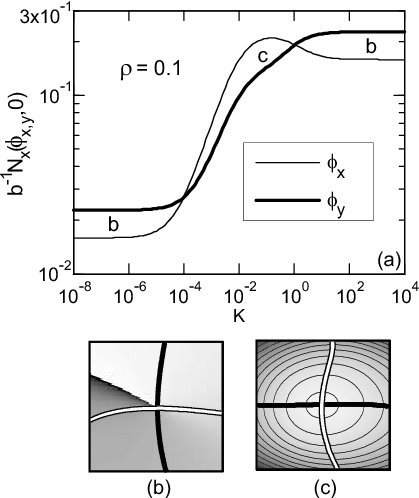
Figure 9: (a) Densities of zero level crossing with the $x$-axis for two disks (DD).  Thin curve, $b^{-1}N_{x}^{\left(\text{DD}\right)}\left(\varphi_{x},0\right)$, Eq. (39), thick curve, $b^{-1}N_{x}^{\left(\text{DD}\right)}\left(\varphi_{y},0\right)$, Eq. (40).  Here $\rho=a/b=0.1$.  (b),(c) Zero crossings Z_x of $\varphi_{x}$ ( Z_y of $\varphi_{y}$), shown as thick white (black) lines, superimposed on a map of (b) a phase vortex, (c) a phase maximum.  In both (b) and (c) the phase increases $0-2\pi$ black to white.  For vortices, Z_x (Z_y) is always strictly parallel (perpendicular) to the $x$-axis.  For extrema, the orientation of these zero crossings depends on the anisotropy and orientation of the elliptical contours in the immediate vicinity of the extremum.  For circular contours, and for elliptical contours whose principal axes parallel the $xy$-axis system, Z_x (Z_y) is parallel to the $y$-axis ($x$-axis).  For other cases there is a strong bias towards an orientation in which the absolute value of the angle that Z_x (Z_y) makes with the $x$-axis is greater than (less than) $45^{o}$.  

Relationship between densities of phase critical points and zero crossings of phase derivatives.

Eq. (38) does not strictly apply to Z_x and Z_y separately, nonetheless, because the differences in $N_{x,x}$ and $N_{x,y}$ are not severe, and in light of the explanation given above for this difference, we can reasonably assume that Eq. (38) does apply, at least approximately, to the average $x$-axis crossing density

$$\left\langle N_{x}^{\left(\text{T}_{a}\text{T}_{b}\right)}\right\rangle\equiv\frac{1}{2}\left(N_{x}^{\left(\text{T}_{a}\text{T}_{b}\right)}\left(\varphi_{x},0\right)+N_{x}^{\left(\text{T}_{a}\text{T}_{b}\right)}\left(\varphi_{y},0\right)\right).$$ (42)

Because all phase critical points - extrema, saddles, and vortices - lie on intersections of Z_x and Z_y, one can reasonably expect some relationship to exist between the densities of these zero lines and the density of critical points.  We therefore attempt to find a relationship between the total phase critical point density $V+E+S=2S$, Eqs. (13) and (14), and $\left\langle N_{x}^{\left(\text{T}_{a}\text{T}_{b}\right)}\right\rangle$.  Noting that $V$, $S$, and $E$ for normal speckle are proportional to $p^{2}$, with $p$ the characteristic inverse length scale of the autocorrelation function, whereas $\left\langle N_{x}\right\rangle$ is proportional to $p$, we make the simplest possible ansatz

$$\sqrt{\left(V+E+S\right)^{\left(\text{T}_{a}\text{T}_{b}\right)}} \approx\frac{1}{2}\left(c^{\left(\text{T}_{a}\right)}+c^{\left(\text{T}_{b}\right)}\right)$$

$$\times b^{-1}\left\langle N_{x}^{\left(\text{T}_{a}\text{T}_{b}\right)}\right\rangle,$$ (43)

where $c^{\left(\text{T}_{a}\right)}$ and $c^{\left(\text{T}_{b}\right)}$ are constants calculated from the single component analog of Eq. (43) (without the factor of $\frac{1}{2})$ for normal $a$ and $b$ speckle fields using the known values of $V$, $E$, $S$, $N_{x,x}$, and $N_{x,y}$ for these fields.  In Fig. 10 we plot the R.H.S. of Eq. (43) as continuous curves on which are superimposed small circles representing the L.H.S of this equation.   Shown are representative results for the case of two Gaussians (GG) and the case where $a$ is a ring and $b$ is a disk (RD).  Other source combinations that are not shown yield similar results.  Considering the wide range of densities ($10^{-4}$ - $1$), the broad parameter range for $K$ ($10^{-12}$ - $10^{4}$), for $\rho$ ($0.001$ - $0.1$), and for $\eta$ ($0.5$ - $10^{5}$, Appendix D), and the fact that there are no adjustable parameters, the agreement with Eq. (43) seems satisfactory.

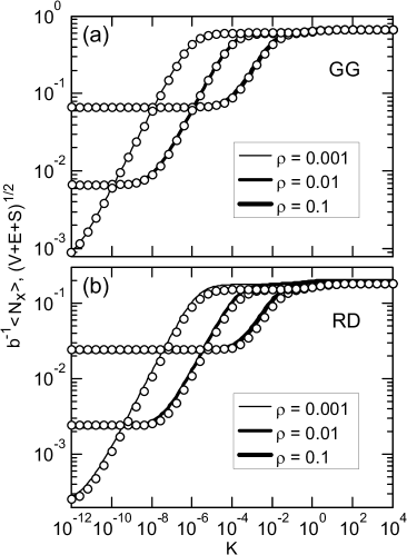
Figure 10: Test of Eq. (43).  The average zero level crossing densities, $b^{-1}\left\langle N_{x}\right\rangle$, are shown by continuous curves, whereas the square roots of the total density of all phase critical points, $\sqrt{V+S+E}$, are shown by small white circles.  In (a) the $a$ and $b$ source fields are both Gaussians (GG).  In (b) the $a$ source field is a ring and the $b$ source field is a disk (RD).

IV CRITICAL POINTS AND ZERO LEVEL CROSSINGS OF THE REAL AND IMAGINARY PARTS OF THE WAVEFUNCTION

The real (imaginary) part of the wavefunction of a speckle pattern represents an archetypal Gaussian random surface.  The critical points that define the major features of such a surface are its extrema (maxima plus minima), saddle points, and umbilic points, the latter being points of isotropic curvature; these are frequently located on the sloping sides of extrema.  Here we study the number densities of these features, and the densities of the associated level crossings, for speckled speckle.  In what follows we consider the real ($\mathcal{R}$) part of the wavefunction, but all results hold equally well for the imaginary ($\mathcal{I}$) part.

IV.1 Critical Points

General results.

The number density $\mathcal{E}$ of extrema [$19$], and the density $\mathcal{U}$ of umbilics [$20$], in normal speckle is extended by inspection to speckled speckle as

$$\mathcal{E}^{\left(\text{T}_{a}\text{T}_{b}\right)}=\frac{1}{3\sqrt{3}\pi}\frac{r_{4}^{\left(\text{T}_{a}\text{T}_{b}\right)}}{r_{2}^{\left(\text{T}_{a}\text{T}_{b}\right)}},$$ (44)

$$\mathcal{U}^{\left(\text{T}_{a}\text{T}_{b}\right)}=\frac{1}{4\pi}\frac{M_{6}^{\left(\text{T}_{a}\text{T}_{b}\right)}}{M_{4}^{\left(\text{T}_{a}\text{T}_{b}\right)}}.$$ (45)

Results for single sources.

For normal speckle [$19,20$] Eqs. (44) and (45) with $k=0$, yield

$$\mathcal{U}^{\left(\text{G}\right)} =\frac{3}{\pi}p^{2},\;\mathcal{E}^{\left(\text{G}\right)}=\frac{2\sqrt{3}}{3\pi}p^{2},$$ (46a)

$$\mathcal{U}^{\left(\text{D}\right)} =\frac{3}{16\pi}p^{2},\;\mathcal{E}^{\left(\text{D}\right)}=\frac{\sqrt{3}}{18\pi}p^{2},$$ (46b)

$$\mathcal{U}^{\left(\text{D}\right)} =\frac{1}{4\pi}p^{2},\;\mathcal{E}^{\left(\text{D}\right)}=\frac{1}{4\sqrt{3}\pi}p^{2}.$$ (46c)

where $$1/p \mathcal{U}/\mathcal{E} 2.6 1.9 1.7$$ is the characteristic length scale in the speckle pattern, Eqs. (9). The number density ratios for a Gaussian (G), disk (D), and ring (R), are , , and , respectively.  Thus, in normal speckle each extremum (maximum or minimum) is decorated by approximately one umbilic point; for speckled speckle, however, the number of umbilic points per extremum can be arbitrarily large, as we now show.

Anomalous ratio of umbilic points to extrema in speckled speckle.

Using Eqs. (44) and (45) we find that for any given small value of $\rho=a/b$, when $K=\mathcal{K}_{\max}^{\left(\text{T}_{a}\text{T}_{b}\right)}$, $\left(\mathcal{U}/\mathcal{E}\right)_{\max}^{\left(\text{T}_{a}\text{T}_{b}\right)}=\left(\mathcal{U}^{\left(\text{T}_{a}\text{T}_{b}\right)}/\mathcal{E}^{\left(\text{T}_{a}\text{T}_{b}\right)}\right)_{\max}$ attains a large, maximum value, where to leading order,

$$\mathcal{K}_{\max}^{\left(\text{T}_{a}\text{T}_{b}\right)} =\frac{c_{4}^{\left(\text{T}_{a}\right)}}{c_{2}^{\left(\text{T}_{a}\right)}}\rho^{4},$$ (47a)

$$\left(\mathcal{U}/\mathcal{E}\right)_{\max}^{\left(\text{T}_{a}\text{T}_{b}\right)} =\frac{9\sqrt{3}}{40}\left(\frac{c_{2}^{\left(\text{T}_{a}\right)}c_{6}^{\left(\text{T}_{a}\right)}}{c_{4}^{\left(\text{T}_{a}\right)}c_{4}^{\left(\text{T}_{b}\right)}}\right)\frac{1}{\rho^{2}},$$ (47b)

with $$c_{2n} n=1,2,3 a b \mathcal{K}_{\max}^{\left(\text{RG}\right)}=\frac{3}{16}\rho^{4} \left(\mathcal{U}/\mathcal{E}\right)_{\max}^{\left(\text{RG}\right)}=3\sqrt{3}/\rho^{2}$$, , given in Eqs. (64).  As an example, for a ring and a Gaussian, , and .

For T = G, D, R, $\left(\mathcal{U}/\mathcal{E}\right)_{\max}^{\left(\text{TT}\right)}/\left(\mathcal{U}/\mathcal{E}\right)^{\left(\text{T}\right)}=1/\left(4\rho^{2}\right)$. For $\rho=0.1$, for example, the ratio of umbilic points to extrema is therefore enhanced by a factor of $25$.

In Fig. 11(a) we plot $\mathcal{U}$, $\mathcal{E}$, and $\mathcal{U}/\mathcal{E}$ for two Gaussians (GG) for $\rho=0.1$.  As can be seen, both $\mathcal{U}$ and $\mathcal{E}$ extrapolate smoothly between their limiting $a$ and $b$ field values, whereas $\mathcal{U}/\mathcal{E}$ shows the expected large peak at $K=10^{-4}$.  These curves are representative, and similar results are obtained for other GDR combinations.  In Figs. 11(b) and (c) we show the real part $\mathcal{R}$ of the wavefield with its umbilic points superimposed.  These points were located using the fact that they lie at the intersections of the zero [$20$] lines of the Stokes-like parameters $\Sigma_{1}$ and $\Sigma_{2}$, where

$$\Sigma_{1} =\mathcal{R}_{xx}-\mathcal{R}_{yy},$$ (48a)

$$\Sigma_{2} =2\mathcal{R}_{xy},$$ (48b)

and the subscripts imply differentiation with respect to $$x y$$ and .

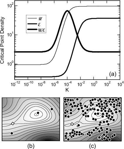
Figure 11: Extrema and umbilic points for two Gaussians (GG) for $\rho=a/b=0.1$.  (a) Densities $\mathcal{U}$ of umbilic points, $\mathcal{E}$ of extrema, and their ratio $\mathcal{U}/\mathcal{E}$.  (b),(c) Gray scale coded contour maps of the real part of the wavefunction $\mathcal{R}$ with superimposed umbilic points (small black circles).  $\mathcal{R}$ increases black to white; the small white diamond marks a saddle point.  (b) $I_{b}=0$ ($K=0$).   (c) $I_{b}/I_{a}=10^{-6}$ ($K=10^{-4}$).  Note that the underlying stationary point structure (extrema and saddle point) in (b) and (c) are very nearly the same.  This is typical, and even for $K\sim 1$ the underlying stationary point structure of the $a$ field remains visible  The $152$ umbilic points in (c), which corresponds to the peak of $\mathcal{U}/\mathcal{E}$ in (a), are consistent with the number expected for a region that contains a central extremum (here a maximum), and parts of the sloping sides of two other extrema (here minima located in the upper left and lower right corners of the figure).  The hyperbolic curvature of the saddle point tends to inhibit formation of umbilic points because the principal radii of curvature of the saddle have opposite signs, whereas at an umbilic point both radii must be equal.     

IV.2 Zero Level Crossings

General results.

Level crossing densities for $\mathcal{R}$, and its first, $\mathcal{R}_{x},\mathcal{R}_{y}$, and second, $\mathcal{R}_{xx},\mathcal{R}_{xy},\mathcal{R}_{yy}$, derivatives have long been known for normal speckle [$17,21$], and we obtain by inspection for level zero for speckled speckle,

$$\mathcal{N}_{0}^{\left(\text{T}_{a}\text{T}_{b}\right)} \equiv\mathcal{N}_{x}^{\left(\text{T}_{a}\text{T}_{b}\right)}\left(\mathcal{R},0\right)=\frac{1}{\pi}\sqrt{r_{2}^{\left(\text{T}_{a}\text{T}_{b}\right)}},$$ (49a)

$$\mathcal{N}_{1}^{\left(\text{T}_{a}\text{T}_{b}\right)} \equiv\mathcal{N}_{x}^{\left(\text{T}_{a}\text{T}_{b}\right)}\left(\mathcal{R}_{x},0\right)=\frac{1}{\pi}\sqrt{r_{4}^{\left(\text{T}_{a}\text{T}_{b}\right)}/r_{2}^{\left(\text{T}_{a}\text{T}_{b}\right)}},$$ (49b)

$$\mathcal{N}_{2}^{\left(\text{T}_{a}\text{T}_{b}\right)} \equiv\mathcal{N}_{x}^{\left(\text{T}_{a}\text{T}_{b}\right)}\left(\mathcal{R}_{xx},0\right)=\frac{1}{\pi}\sqrt{r_{6}^{\left(\text{T}_{a}\text{T}_{b}\right)}/r_{4}^{\left(\text{T}_{a}\text{T}_{b}\right)}},$$ (49c)

and

$$\mathcal{N}_{x}^{\left(\text{T}_{a}\text{T}_{b}\right)}\left(\mathcal{R}_{y},0\right) =\frac{1}{\sqrt{3}}\mathcal{N}_{x}^{\left(\text{T}_{a}\text{T}_{b}\right)}\left(\mathcal{R}_{x},0\right),$$ (50a)

$$\mathcal{N}_{x}^{\left(\text{T}_{a}\text{T}_{b}\right)}\left(\mathcal{R}_{xy},0\right) =\sqrt{\frac{3}{5}}\mathcal{N}_{x}^{\left(\text{T}_{a}\text{T}_{b}\right)}\left(\mathcal{R}_{xx},0\right),$$ (50b)

$$\mathcal{N}_{x}^{\left(\text{T}_{a}\text{T}_{b}\right)}\left(\mathcal{R}_{yy},0\right) =\sqrt{\frac{1}{5}}\mathcal{N}_{x}^{\left(\text{T}_{a}\text{T}_{b}\right)}\left(\mathcal{R}_{xx},0\right).$$ (50c)

For the ratios of zero crossing densities we have

$$\mathcal{N}_{1,0}^{\left(\text{T}_{a}\text{T}_{b}\right)}\equiv\frac{\mathcal{N}_{1}^{\left(\text{T}_{a}\text{T}_{b}\right)}}{\mathcal{N}_{0}^{\left(\text{T}_{a}\text{T}_{b}\right)}}=\sqrt{\eta^{\left(\text{T}_{a}\text{T}_{b}\right)}+1},$$ (51)

where $\eta^{\left(\text{T}_{a}\text{T}_{b}\right)}$ is given in Appendix D, and

$$\mathcal{N}_{2,1}^{\left(\text{T}_{a}\text{T}_{b}\right)}\equiv\frac{\mathcal{N}_{2}^{\left(\text{T}_{a}\text{T}_{b}\right)}}{\mathcal{N}_{1}^{\left(\text{T}_{a}\text{T}_{b}\right)}}=\frac{\sqrt{10}}{3^{3/4}}\sqrt{\frac{\mathcal{U}^{\left(\text{T}_{a}\text{T}_{b}\right)}}{\mathcal{E}^{\left(\text{T}_{a}\text{T}_{b}\right)}}}.$$ (52)

Results for single sources.

In normal speckle fields zero crossings of $R$, $R_{x}$, and $R_{xx}$ have similar densities.  Setting $K=0$ ($I_{b}=0$) in Eqs. (51) and (52), we have in obvious notation

$$\mathcal{N}_{1,0}^{\left(\text{G}\right)} =\sqrt{3}\approx 1.73,\;\mathcal{N}_{2,1}^{\left(\text{G}\right)}=\sqrt{5/3}\approx 1.29,$$ (53a)

$$\mathcal{N}_{1,0}^{\left(\text{D}\right)} =\sqrt{2}\approx 1.41,\;\mathcal{N}_{2,1}^{\left(\text{G}\right)}=\sqrt{5}/2\approx 1.12,$$ (53b)

$$\mathcal{N}_{1,0}^{\left(\text{R}\right)} =\sqrt{3/2}\approx 1.22,\;\mathcal{N}_{2,1}^{\left(\text{R}\right)}=\sqrt{10}/3\approx 1.05,$$ (53c)

For speckled speckle, however, these ratios can be arbitrarily large, as we now show.

Anomalous ratios for compound sources.

$\mathcal{N}_{1,0}^{\left(\text{T}_{a}\text{T}_{b}\right)}$, Eq. (51), and $\mathcal{N}_{2,1}^{\left(\text{T}_{a}\text{T}_{b}\right)}$, Eq. (52), can be made arbitrarily large by a suitable choice of $K^{\left(\text{T}_{a}\text{T}_{b}\right)}$ and $\rho$.  For $\mathcal{N}_{1,0}^{\left(\text{T}_{a}\text{T}_{b}\right)}$ we find that for any given small value of $\rho$, when $K^{\left(\text{T}_{a}\text{T}_{b}\right)}=\left(\mathcal{K}_{1,0}^{\left(\text{T}_{a}\text{T}_{b}\right)}\right)_{\max}$, $\mathcal{N}_{1,0}^{\left(\text{T}_{a}\text{T}_{b}\right)}$ attains a maximum value, $\left(\mathcal{N}_{1,0}^{\left(\text{T}_{a}\text{T}_{b}\right)}\right)_{\max}$, where to leading order in $\rho$,

$$\left(\mathcal{K}_{1,0}^{\left(\text{T}_{a}\text{T}_{b}\right)}\right)_{\max} =\frac{c_{2}^{\left(\text{T}_{a}\right)}}{c_{2}^{\left(\text{T}_{b}\right)}}\rho^{2},$$ (54a)

$$\left(\mathcal{N}_{1,0}^{\left(\text{T}_{a}\text{T}_{b}\right)}\right)_{\max} =\frac{1}{2\rho}\sqrt{\frac{c_{4}^{\left(\text{T}_{b}\right)}}{c_{2}^{\left(\text{T}_{a}\right)}c_{2}^{\left(\text{T}_{b}\right)}}}.$$ (54b)

Similarly, for $$\mathcal{N}_{2,1}^{\left(\text{T}_{a}\text{T}_{b}\right)}$$ we find

$$\left(\mathcal{K}_{2,1}^{\left(\text{T}_{a}\text{T}_{b}\right)}\right)_{\max} =\frac{c_{4}^{\left(\text{T}_{a}\right)}}{c_{4}^{\left(\text{T}_{b}\right)}}\rho^{4},$$ (55a)

$$\left(\mathcal{N}_{2,1}^{\left(\text{T}_{a}\text{T}_{b}\right)}\right)_{\max} =\frac{1}{2\rho}\sqrt{\frac{c_{2}^{\left(\text{T}_{a}\right)}c_{6}^{\left(\text{T}_{b}\right)}}{c_{4}^{\left(\text{T}_{a}\right)}c_{4}^{\left(\text{T}_{b}\right)}}}.$$ (55b)

As representative examples we plot in Fig. 12 $$\mathcal{N}_{1,0}^{\left(\text{GG}\right)} \mathcal{N}_{2,1}^{\left(\text{GG}\right)} \rho=0.01$$ and for .  As can be seen, both densities show large enhancements at their peaks over their normal speckle values.  Below we inquire as to the sources of these enhancements.

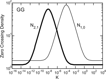
Figure 12: Zero crossing densities $N_{1,0}^{\left(GG\right)}$, Eq. (54b), and $N_{2,1}^{\left(GG\right)}$, Eq. (55b), for two Gaussians (GG) for $\rho=0.01$.  For this value of $\rho$, $N_{1,0}^{\left(GG\right)}$ ($N_{2,1}^{\left(GG\right)}$) is enhanced at its peak, $K=10^{-4}$ ($K=10^{-8}$), by a factor of $50$ ($44$) over its normal speckle value, Eqs. (53a).

$\mathcal{N}_{1,0}^{\left(\text{T}_{a}\text{T}_{b}\right)}$.

The zero crossings of $\mathcal{R}$, which obey Eq. (38), divide the field into nodal domains of opposite sign.  In normal speckle maxima (minima) mostly occupy positive (negative) domains. $\mathcal{N}_{x}\left(\mathcal{R},0\right)$ therefore roughly scales with the square root of the density of extrema.  The same is true for $\mathcal{N}_{x}\left(\mathcal{R}_{x},0\right)$, because extrema (and saddles) lie at intersections of $\mathcal{R}_{x}$ and $\mathcal{R}_{y}$.  Accordingly, in normal speckle $\mathcal{N}_{x}\left(\mathcal{R}_{x},0\right)\sim\mathcal{N}_{x}\left(\mathcal{R},0\right)$, Eqs. (53).  In speckled speckle, however, the situation is very different.

For vanishingly small $K$ the only extrema are those of the $a$ field, and the nodal domains of $\mathcal{R}$ are determined by these extrema. As $K$ increases, however, numerous very small amplitude extrema associated with the presence of the $b$ field (here colloquially “$b$ extrema”) begin to appear.  These $b$ extrema decorate with equal probability both positive and negative nodal domains of $\mathcal{R}$, but because of their very small amplitudes they do not divide up these nodal domains.  Thus, $\mathcal{N}_{0}=\mathcal{N}_{x}\left(\mathcal{R},0\right)$ is not significantly increased by the presence of the $b$ extrema.  $\mathcal{N}_{1}=\mathcal{N}_{x}\left(\mathcal{R}_{x},0\right)$, however, is increased in proportion to the square root of the density of these extrema, because $\mathcal{R}_{x}$ (and $\mathcal{R}_{y}$) goes to zero at an extremum no matter how small its amplitude.  As a result, $\mathcal{N}_{1,0}=$ $\mathcal{N}_{1}/\mathcal{N}_{0}$ begins to grow with $K$.  This growth continues until the amplitude of the $b$ source field is such that the amplitudes of the $b$ extrema become large enough to carve up the nodal domains of $\mathcal{R}$ into small regions.  When this happens $\mathcal{N}_{0}$ begins to grow rapidly.  Thus the peak in $\mathcal{N}_{1,0}$ is due to an initial growth of $\mathcal{N}_{1}$ with no significant growth in $\mathcal{N}_{0}$, followed by a leveling off of $\mathcal{N}_{1}$ together with rapid growth in $\mathcal{N}_{0}$.  This scenario, which applies to all GDR source combinations, is illustrated in Fig. 13.

$\mathcal{N}_{2,1}^{\left(\text{T}_{a}\text{T}_{b}\right)}$.

Why is $\mathcal{N}_{2}=\mathcal{N}_{x}\left(\mathcal{R}_{xx},0\right)$ for speckled speckle so much larger than $\mathcal{N}_{1}=\mathcal{N}_{x}\left(\mathcal{R}_{x},0\right)$, when for normal speckle the two are nearly equal, Eqs. (53)?  The answer is analogous to the reason, discussed above, why in speckled speckle $\mathcal{N}_{1}$ is so much larger than $\mathcal{N}_{0}$, even though in normal speckle also these two densities are nearly equal.

As discussed at the beginning of this section, for very small $K$ each extremum is decorated on average by a single umbilic point, but as $K$ increases the number of umbilics/extremum increases rapidly, Eqs. (47) and Fig. 11.  Now, at an umbilic point $\mathcal{R}_{xx}=\mathcal{R}_{yy}$ and $\mathcal{R}_{xy}=0$ [$20$].  Accordingly, as the number of umbilics increases so does $\mathcal{N}_{x}\left(\mathcal{R}_{xy},0\right)$, the number of zero crossings of $\mathcal{R}_{xy}$.  But for the circular Gaussian statistics relevant here $\mathcal{N}_{2}=\sqrt{5/3}\mathcal{N}_{x}\left(\mathcal{R}_{xy},0\right)$, Eq. (50b), so that as the number of umbilics increases so also does $\mathcal{N}_{2}$.  The net result is that because $\mathcal{N}_{2}$ increases rapidly with the number of umbilics, whereas $\mathcal{N}_{1}$ increases more slowly, only with the number of extrema (Fig. 13), $\mathcal{N}_{2}/\mathcal{N}_{1}$ peaks at some intermediate value of $K$.  These considerations could be illustrated by the analog of Fig. 13 in which $\mathcal{N}_{0}$ is replaced by $\mathcal{N}_{1}$, $\mathcal{N}_{1}$ by $\mathcal{N}_{2}$, and $\mathcal{N}_{1,0}$ by $\mathcal{N}_{2,1}$; we refrain from presenting the resulting figure, however, because except for scaling factors it is very similar to Fig. 13.

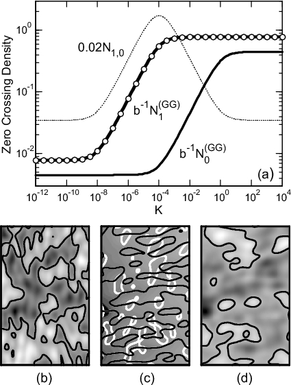
Figure 13: (a) Zero crossings densities $b^{-1}N_{1}$ (thick curve) and $b^{-1}N_{0}$ (thin curve) vs. $K$ for $a$ and $b$ fields Gaussians (GG) with $\rho=a/b=0.01$.  $N_{0}$ ($N_{1}$) is given in Eq. (49a), (Eq. (49b)).  The small white circles are the square root of the scaled density $\mathcal{E}$ of extrema calculated from the exact result $\sqrt{\mathcal{E}\left(K\right)}=\left(\sqrt{\pi}/3^{3/4}\right)N_{1}\left(K\right)$, where $\mathcal{E}$ is given in Eq. (44).   The dotted curve is $N_{1,0}=N_{1}/N_{0}$ rescaled to permit easy comparison with curves $b^{-1}N_{0}$ and $b^{-1}N_{1}$.  (b)-(d) Gray scale coded maps of $\mathcal{R}\left(x,y\right)$ for $\rho=0.01$ for different values of $K$.  In all maps $\mathcal{R}$ increases black to white. (b) $K=10^{-4}$.  The thick curves are zero crossings of $\mathcal{R}$ that divide the field into positive/negative nodal domains.  As can be seen, maxima (minima) almost invariably lie in positive (negative) domains.  Maps for $K<10^{-4}$ differ negligibly from the one shown here.  (c) The central region in (b) enlarged by a factor of $100$, so that the area shown is $10^{-4}$ the area in (b).  Thick white (black) curves are zero crossings of derivatives $\mathcal{R}_{x}$ ($\mathcal{R}_{y}$). Every intersection of $\mathcal{R}_{x}$ and $\mathcal{R}_{y}$ marks a stationary point - extremum or saddle point; on average there are equal numbers of each type.  Here the amplitudes of the extrema are so small that they are not apparent visually.  (d) The region in (c) for $K=1$.  Thick curves are zero crossings of $\mathcal{R}$.  Here the extrema have large amplitudes.  Because of this they are not only visible, but they also divide each nodal domain in (b) into some $10^{4}$ small domains.  Maps for $K>1$ differ unimportantly from the one shown here.  

V SUMMARY

A priori, one might reasonably expect that adding a weak random field, the $b$ field, onto a strong random field, the $a$ field, would result in only minor perturbations of the $a$ field structure and statistics.  The opposite was found to be true, however, and just about every structural and statistical property of the combined field was shown to display large anomalies when the optical power $P_{b}$ of the $b$ field is some $10^{-4}$ - $10^{-6}$ the power $P_{a}$ of the $a$ field; these anomalies of speckled speckle are summarized below for $\rho=a/b=10^{-1}$ - $10^{-2}$.

(i) Singularity clustering:  Vortices in scalar fields and C points in vector fields cluster in the dark regions surrounding the bright speckle spots of the $a$ field; the reason is that singularity formation requires equal amplitudes for the $a$ and $b$ fields.

(ii) Phase field statistics:  In both scalar and vector fields extrema can outnumber singularities by orders of magnitude; in contrast, in normal speckle singularities always outnumber extrema.

(a) Scalar fields.  For a sufficiently weak $b$ field, say $P_{b}/P_{a}\sim 10^{-8}$ - $10^{-10}$, extrema and vortices maintain their normal ratio.  But as $P_{b}$ grows, the number density of extrema, $E$, grows faster than the density, $V$, of vortices, and the ratio $E/V$ can become orders of magnitude larger than normal.  When $P_{b}/P_{a}\gg 1$, the $E/V$ ratio returns to its normal value.  Thus, $E/V$ is normal for both very small and very large $P_{b}/P_{a}$, and peaks at some still small, intermediate value of $P_{b}/P_{a}$.

(b) Vector fields.  For all nonzero $P_{b}$ less than some critical value $P_{b}^{0}$, the ratio of the number density of azimuthal extrema, $\mathbb{E}$, can exceed the number density, $\mathbb{V}$, of C points (Stokes vortices) by orders of magnitude.  For $P_{b}<P_{b}^{0}$, $\mathbb{E}/\mathbb{V}$ is essentially independent of $P_{b}$ and is substantially equal to half the maximum scalar field ratio $E/V$ for the same value of $\rho$; $P_{b}^{0}$ approximately equals $P_{b}$ at the peak of $E/V$.  When $P_{b}/P_{a}\gg 1$, $\mathbb{E}/\mathbb{V}$ returns to its normal value.  Thus, $\mathbb{E}/\mathbb{V}$ is large for small $P_{b}$ and small for large $P_{b}$.

(iii) Phase field derivative zero crossings: The ratio of the density of $x$-derivative zero crossings to $y$-derivative zero crossings changes anomalously with $P_{b}$; this anomaly is explained by the anomalous $E/V$ ratio and the differences in the geometry of the zero crossings at vortices and at extrema.

(iv) Real and imaginary parts of the wave function:

(a) Umbilic points.  For a sufficiently weak $b$ field, say $P_{b}/P_{a}\sim 10^{-10}$ - $10^{-12}$, extrema and umbilic points maintain their normal $\sim 1:1$ ratio.  But as $P_{b}$ is increased, the number density of extrema, $\mathcal{E}$, grows faster than the density, $\mathcal{U}$, of umbilic points, and the ratio $\mathcal{E}/\mathcal{U}$ can become orders of magnitude larger than normal.  $\mathcal{E}/\mathcal{U}$ returns to its normal value when $P_{b}/P_{a}\gg 1$.

(b) Nodal domains and derivative zero crossings. The densities of the zero crossings that define nodal domains and the densities of the zero crossings of all first and second order derivatives show anomalously large ratios.  These anomalous ratios are explained by the anomalous $\mathcal{E}/\mathcal{U}$ ratio and the relationships of the different zero crossings to extrema and umbilic points.

In general, the anomalous ratios of critical point densities occur because the number density of one wavefield feature grows rapidly with an increase in the power of the $b$ field while the growth rate of a second feature lags behind.  Such an imbalance in growth rates can be expected to be the norm, and other properties of speckled speckle, including properties that defy calculation, can be expected to show large anomalies; these anomalies can, and should be, sought experimentally.

Appendix A Composite Field Autocorrelation Function

Returning to the derivation of the autocorrelation functions of the simple sources in Eqs. (6a)-(6c) we write $W$ in terms of the numerator $N\left(pr\right)$ and denominator $D\left(p\right)$ of Eq. (4) as

$$W\left(pr\right)=N\left(pr\right)/D\left(p\right),$$ (56)

where for the Gaussian (G), disk (D), and ring (R):

$$N^{\left(\text{G}\right)}\left(pr\right) =2p^{2}exp\left(-p^{2}r^{2}\right),\;D^{\left(\text{G}\right)}\left(p\right)=2p^{2};$$ (57a)

$$N^{\left(\text{D}\right)}\left(pr\right) =p^{2}J_{1}\left(pr\right)/\left(pr\right),\;D^{\left(\text{D}\right)}\left(p\right)=p^{2}/2;$$ (57b)

$$N^{\left(\text{R}\right)}\left(pr\right) =\varepsilon pJ_{0}\left(pr\right),\;D^{\left(\text{R}\right)}\left(p\right)=\varepsilon p.$$ (57c)

Inserting Eqs. (57a)-(57c) into Eq. (56) immediately leads to Eqs. (9a)-(9c).

The numerator (denominator) of the composite autocorrelation function in Eq. (4) is a linear combination of the $N$ ($D$) in Eqs. (57a)-(57c) with $p$ replaced by $a$ or $b$, as required. Inserting the appropriate combinations of $N$ and $D$ into Eq. (4) leads to Eq. (12) with

$$K^{\left(\text{T}_{a}\text{T}_{b}\right)}=P_{b}^{\left(\text{T}_{b}\right)}/P_{a}^{\left(\text{T}_{a}\right)},$$ (58)

with $P_{a}^{\left(\text{T}_{a}\right)}$ ($P_{b}^{\left(\text{T}_{b}\right)}$) the total optical power in source $a$ ($b$).  For a Gaussian (G), disk (D), and ring (R),

$$P_{p}^{\left(\text{G}\right)} =4\pi p^{2}I_{p},$$ (59a)

$$P_{p}^{\left(\text{D}\right)} =\pi p^{2}I_{p},$$ (59b)

$$P_{p}^{\left(\text{R}\right)} =2\pi p\varepsilon I_{p},$$ (59c)

where $$\ p=a,b. I_{p} I_{p} I_{p}$$  For a Gaussian is the peak intensity at the center of the source profile, for a disk is the uniform source intensity within the disk, and for a ring is the uniform source intensity within the narrow annulus.

As a specific example, for a composite source with $a$ a Gaussian and $b$ a ring,

$$W^{\left(\text{GR}\right)}\left(r\right) =\dfrac{\exp\left(-a^{2}r^{2}\right)+K^{\left(\text{GR}\right)}J_{0}\left(br\right)}{1+K^{\left(\text{GR}\right)}},$$

$$K^{\left(\text{GR}\right)} =b\varepsilon I_{b}/2a^{2}I_{a}.$$

Appendix B Derivatives

The autocorrelation function $\mathcal{W}$ of $\mathcal{R}$ (or equivalently of $\mathcal{I}$) is

$$\mathcal{W}\left(pr\right) =\left\langle\mathcal{R}\left(0\right)\mathcal{R}\left(pr\right)\right\rangle/\left\langle\mathcal{R}^{2}\right\rangle,$$ (60a)

$$=\left\langle\mathcal{I}\left(0\right)\mathcal{I}\left(pr\right)\right\rangle/\left\langle\mathcal{I}^{2}\right\rangle,$$ (60b)

$$=\left\langle\mathcal{R}^{2}\right\rangle W\left(pr\right)=\left\langle\mathcal{I}^{2}\right\rangle W\left(pr\right).$$ (60c)

Suppressing momentarily for notational simplicity superscripts T,

$$r_{2n} \equiv\left\langle\mathcal{R}_{n}^{2}\right\rangle/\left\langle\mathcal{R}^{2}\right\rangle,$$ (61a)

$$\left\langle\mathcal{R}_{n}^{2}\right\rangle =\left(-1\right)^{n}\left(\frac{d^{2n}\mathcal{W}\left(pr\right)}{dr^{2n}}\right)_{r=0}.$$ (61b)

Reintroducing superscripts T,

$$r_{2n}^{\left(\text{T}_{a}\text{T}_{b}\right)}=\frac{r_{2n}^{\left(\text{T}_{a}\right)}+K^{\left(\text{T}_{a}\text{T}_{b}\right)}r_{2n}^{\left(\text{T}_{b}\right)}}{1+K^{\left(\text{T}_{a}\text{T}_{b}\right)}},$$ (62)

where

$$r_{2n}^{\left(\text{T}\right)}=c_{2n}^{\left(\text{T}\right)}p^{2n}.$$ (63)

For the Gaussian (G), disk (D), and ring (R):

$$c_{2}^{\left(\text{G}\right)} =2,\;c_{4}^{\left(\text{G}\right)}=12,\;c_{6}^{\left(\text{G}\right)}=120;$$ (64a)

$$c_{2}^{\left(\text{D}\right)} =1/4,\;c_{4}^{\left(\text{D}\right)}=1/8,\;c_{6}^{\left(\text{D}\right)}=5/64;$$ (64b)

$$c_{2}^{\left(\text{R}\right)} =1/2,\;c_{4}^{\left(\text{R}\right)}=3/8,\;c_{6}^{\left(\text{R}\right)}=5/16.$$ (64c)

Defining derivatives $\mathfrak{r}_{2n}^{\left(\text{R}\right)}$ for the annulus in Eq. (10a) using Eq. (61b), to leading order in the small quantity $\varepsilon/p$,

$$\mathfrak{r}_{2}^{\left(\text{R}\right)}/r_{2}^{\left(\text{R}\right)} =1+\left(1/4\right)\left(\varepsilon^{2}/p^{2}\right),$$ (65a)

$$\mathfrak{r}_{4}^{\left(\text{R}\right)}/r_{4}^{\left(\text{R}\right)} =1+\left(5/6\right)\left(\varepsilon^{2}/p^{2}\right),$$ (65b)

$$\mathfrak{r}_{6}^{\left(\text{R}\right)}/r_{6}^{\left(\text{R}\right)} =1+\left(7/4\right)\left(\varepsilon^{2}/p^{2}\right).$$ (65c)

For $$\varepsilon/p=0.1 \varepsilon/p=0.01 10^{-4}$$, for the various quantities calculated in the text the differences between the experimentally realizable annulus and the theoretical ring are therefore less than a few percent, whereas for these differences are of order .

As a specific example for, say, $r_{4}$, for a composite source with $a$ a ring and $b$ a disk,

$r_{4}^{\left(\text{RD}\right)}=\left(3a^{4}/8+K^{\left(\text{RD}\right)}b^{4}/8\right)/\left(1+K^{\left(\text{RD}\right)}\right).$

Appendix C Moments

The moments $M_{2n}$ of the source function $S$ are defined for a composite source by

$$M_{2n}^{\left(\text{T}_{a}\text{T}_{b}\right)}=\dfrac{\int_{0}^{\infty}u^{2n+1}S^{\left(\text{T}_{a}\text{T}_{b}\right)}\left(u\right)du}{\int_{0}^{\infty}uS^{\left(\text{T}_{a}\text{T}_{b}\right)}\left(u\right)du}.$$ (66)

Expanding both $W\left(pr\right)$ and $J_{0}\left(ur\right)$ in Eq. (4),

$$M_{2n}^{\left(\text{T}_{a}\text{T}_{b}\right)}=\frac{\left(n!\right)^{2}4^{n}}{\left(2n\right)!}r_{2n}^{\left(\text{T}_{a}\text{T}_{b}\right)}.$$ (67)

It is useful to express $M_{2n}^{\left(\text{T}_{a}\text{T}_{b}\right)}$ for speckled speckle in a form that parallels Eq. (12),

$$M_{2n}^{\left(\text{T}_{a}\text{T}_{b}\right)}=\frac{M_{2n}^{\left(\text{T}_{a}\right)}\left(a\right)+K^{\left(\text{T}_{a}\text{T}_{b}\right)}M_{2n}^{\left(\text{T}_{b}\right)}\left(b\right)}{1+K^{\left(\text{T}_{a}\text{T}_{b}\right)}}.$$ (68)

where

$$M_{2n}^{\left(\text{T}\right)}\left(p\right)=m_{2n}^{(\text{T})}p^{2n},$$ (69)

with

$$m_{2}^{\left(\text{T}\right)}=2c_{2}^{\left(\text{T}\right)},\;m_{4}^{\left(\text{T}\right)}=(8/3)c_{4}^{\left(\text{T}\right)},\;m_{6}^{\left(\text{T}\right)}=(16/5)c_{6}^{\left(\text{T}\right)}.$$ (70)

$c_{2n}^{\left(\text{T}\right)}$ is given in Eqs. (64) for a Gaussian (T = G), disk (T = D), and ring (T = R).

As a specific example, for a composite source with $a$ a Gaussian and $b$ a disk,

$M_{6}^{\left(\text{GD}\right)}=\left(384a^{6}+K^{\left(\text{GD}\right)}b^{6}/4\right)/\left(1+K^{\left(\text{GD}\right)}\right)$.

Like the autocorrelation functions, the moments of composite sources are the optical power weighted averages of the moments of the individual sources $a$ and $b$.

Appendix D $\mathbf{\eta}$

We discuss here the dimensionless parameter $\eta$ that plays a central role in the level crossing statistics of derivatives of the phase, of the real and imaginary parts of the wavefunction, and of the intensity.  Extending [$17$], we write for speckled speckle

$$\eta^{\left(\text{T}_{a}\text{T}_{b}\right)}=r_{4}^{\left(\text{T}_{a}\text{T}_{b}\right)}/\left(r_{2}^{\left(\text{T}_{a}\text{T}_{b}\right)}\right)^{2}-1,$$ (71)

where the normalized derivatives $r_{2n}^{\left(\text{T}_{a}\text{T}_{b}\right)}$ are given in Appendix B.  Of special interest is the regime where $\eta^{\left(\text{T}_{a}\text{T}_{b}\right)}$ becomes anomalously large.  We find that $\eta^{\left(\text{T}_{a}\text{T}_{b}\right)}$ reaches a maximum, $\eta_{\max}^{\left(\text{T}_{a}\text{T}_{b}\right)}$, when $K^{\left(\text{T}_{a}\text{T}_{b}\right)}=\mathcal{K}_{\max}^{\left(\text{T}_{a}\text{T}_{b}\right)}$, where

$$\mathcal{K}_{\max}^{\left(\text{T}_{a}\text{T}_{b}\right)} =\frac{c_{2}^{\left(\text{T}_{a}\right)}}{c_{2}^{\left(\text{T}_{b}\right)}}\rho^{2},$$ (72a)

$$\eta_{\max}^{\left(\text{T}_{a}\text{T}_{b}\right)} =\frac{c_{4}^{\left(\text{T}_{b}\right)}}{4c_{2}^{\left(\text{T}_{a}\right)}c_{2}^{\left(\text{T}_{b}\right)}}\left(\frac{1}{\rho^{2}}\right).$$ (72b)

For example, for $$a b$$ a ring (R) and  a disk (D)

$$\mathcal{K}_{\max}^{\left(\text{RG}\right)} =\frac{c_{2}^{\left(\text{R}\right)}}{c_{2}^{\left(\text{D}\right)}}\rho^{2}=2\rho^{2},$$

$$\eta_{\max}^{\left(\text{RG}\right)} =\frac{c_{4}^{\left(\text{D}\right)}}{4c_{2}^{\left(\text{R}\right)}c_{2}^{\left(\text{D}\right)}}\left(\frac{1}{\rho^{2}}\right)=\frac{1}{4\rho^{2}}.$$

For normal speckle, for a Gaussian $\eta=2$, for a disk $\eta=1$, and for a ring $\eta=\tfrac{1}{2}$.  In contrast, for speckled speckle for say $\rho=0.1$, $\eta_{\max}^{\left(\text{GG}\right)}=75$, $\eta_{\max}^{\left(\text{DD}\right)}=50$, and $\eta_{\max}^{\left(\text{RR}\right)}=25$.

References

[1] J. W. Goodman, Speckle Phenomena In Optics (Roberts & Co., Englewood, Colorado, 2007).  A comprehensive review of the properties of normal speckle is given here, together with a very extensive bibliography.

[2] I. Freund and D. A. Kessler, “Singularities in speckled speckle,” Opt. Lett. 33, 479-481 (2008).

[3] D. A. Kessler and I. Freund, “Short- and long-range screening of optical phase singularities and C points,” Opt. Commun. (in press).

[4] M. Berry, “Disruption of wave-fronts: statistics of dislocations in incoherent Gaussian random waves,” J. Phys. A 11, 27-37 (1978).

[5] B. I. Halperin, “Statistical mechanics of topological defects,” in Physics of Defects, R. Balian, M. Kleman, and J.-P. Poirier, Eds. (North-Holland, Amsterdam, 1981), pp. 814-857.

[6] N. B. Baranova, B. Ya Zel’dovich, A. V. Mamaev, N. Pilipetskii and V. V. Shkukov, “Dislocations of the wave-front of a speckle-inhomogeneous field (theory and experiment),” JETP Lett. 33, 195-199 (1981).

[7] M. R. Dennis, “Phase critical point densities in planar isotropic random waves,” J. Phys. A: Math. Gen. 34, L297-L303 (2003).

[8] J. F. Nye and M. V. Berry “Dislocations in wave trains”, Proc. Roy. Soc. Lond. A 336, 165-190 (1974).

[9] J. F. Nye, J. V. Hajnal, and J. H. Hannay, “Phase saddles and dislocations in two-dimensional waves such as the tides,” Proc. Roy. Soc. Lond. A 417, 7-20 (1988).

[10] I. Freund, “Saddles, singularities, and extrema in random phase fields,” Phys. Rev. E 52, 2348-2360 (1995).

[11] M. Born and E. W. Wolf, Principles of Optics (Pergamon Press, Oxford, 1959), Sect. 1.4.2.

[12] J. F. Nye, Natural Focusing and Fine Structure of Light (IOP Publ., Bristol, 1999).

[13] I. Freund, M. S. Soskin, and A. I. Mokhun, “Elliptic critical points in paraxial optical fields,” Opt. Commun. 208, 223-253 (2002).

[14] I. Freund, “Poincaré vortices,” Opt. Lett. 26, 1996-1998 (2001).

[15] M. R. Dennis, “Polarization singularities in paraxial vector fields: morphology and statistics,” Opt. Commun. 145, 201–221 (2002); “Nodal densities of planar gaussian random waves,” Eur. Phys. J. Special Topics 213, 191-210 (2007).

[16] I. Freund, “Vortex derivatives,” Opt. Commun. 137, 118-126 (1997).

[17] D. A. Kessler and I. Freund, “Level-crossing densities in random wave fields,” J. Opt. Soc. Am. A 15, 1608-1618 (1998).

[18] I. Freund, “‘1001’ correlations in random wave fields,” Waves in Random Media 8, 119-158 (1998).

[19] D. E. Cartwright and M. S. Longuet-Higgins, “The statistical distribution of the maxima of a random function,” Proc. R. Soc. Lond., Ser. A 237, 212–232 (1956); M. S. Longuet-Higgins, “Reflection and refraction at a random moving surface: II. Number of specular points in a Gaussian surface,” J. Opt. Soc. Am. 50, 845–850 (1960).

[20] M. V. Berry and J. H. Hannay, “Umbilic points on Gaussian random surfaces”, J. Phys. A 10, 1809-1821 (1977).

[21] S. O. Rice, “Mathematical analysis of random noise,” in Selected Papers on Noise and Stochastic Processes, N. Wax, Ed. (Dover, New York, 1954), pp. 133–294.  Although the planar optical field is two-dimensional, the density of zero crossings along a straight line is a one-dimensional problem.