Correlating radii and electric monopole transitions of atomic nuclei

Abstract

A systematic analysis of the spherical-to-deformed shape phase transition in even-even rare-earth nuclei from ₅₈Ce to ₇₄W is carried out in the framework of the interacting boson model. These results are then used to calculate nuclear radii and electric monopole (E0) transitions with the same effective operator. The influence of the hexadecapole degree of freedom ($g$ boson) on the correlation between radii and E0 transitions thus established, is discussed.

Electric monopole (E0) transitions between nuclear levels proceed mainly by internal conversion with no transfer of angular momentum to the ejected electron. For transition energies greater than $2m_{\rm e}c^{2}$, electron-positron pair creation is also possible; two-photon emission is possible at all energies but extremely improbable. The total probability for a transition between initial and final states $|{\rm i}\rangle$ and $|{\rm f}\rangle$ can be separated into an electronic and a nuclear factor, $P=\Omega\rho^{2}$, where the nuclear factor $\rho$ is Church56

$$\rho=\sum_{p=1}^{Z}\langle{\rm f}|\left(\frac{r_{p}}{R}\right)^{2}-\sigma\left(\frac{r_{p}}{R}\right)^{4}+\cdots|{\rm i}\rangle,$$ (1)

with $R=r_{0}A^{1/3}$ ($r_{0}=1.2$ fm) and where the summation runs over the $Z$ protons in the nucleus. The coefficient $\sigma$ depends on the assumed nuclear charge distribution but in any reasonable case it is smaller than 0.1 and can be neglected if the leading term is not too small Church56 .

The charge radius of a state $|{\rm s}\rangle$ is given by

$$\langle r^{2}\rangle_{\rm s}=\frac{1}{Z}\langle{\rm s}|\sum_{p=1}^{Z}r^{2}_{p}|{\rm s}\rangle.$$ (2)

It is found experimentally that the addition of neutrons produces a change in the nuclear charge distribution, an effect which can be parametrized by means of neutron and proton effective charges $e_{\rm n}$ and $e_{\rm p}$ in the charge radius operator $\hat{T}(r^{2})$. This leads to the following generalization of Eq. (2):

$$\langle r^{2}\rangle_{\rm s}\equiv\langle{\rm s}|\hat{T}(r^{2})|{\rm s}\rangle=\frac{1}{e_{\rm n}N+e_{\rm p}Z}\langle{\rm s}|\sum_{k=1}^{A}e_{k}r^{2}_{k}|{\rm s}\rangle,$$ (3)

where the sum is over all nucleons and $e_{k}=e_{\rm n}$ ($e_{\rm p}$) if $k$ is a neutron (proton).

An obvious connection between $\rho$ and the nuclear charge radius is established in the approximation $\sigma=0$ (which henceforth will be made). Again because of the polarization effect of the neutrons, one introduces an E0 operator of the form Kantele84

$$\hat{T}({\rm E0})=\sum_{k=1}^{A}e_{k}r^{2}_{k}.$$ (4)

The $\rho$ defined in Eq. (1) with $\sigma=0$ is then given by $\rho=\langle{\rm f}|\hat{T}({\rm E0})|{\rm i}\rangle/eR^{2}$. The basic hypothesis of this Letter is to assume that the effective nucleon charges in the charge radius and E0 transition operators are the same. If this is so, comparison of Eqs. (3) and (4) leads to the relation

$$\hat{T}({\rm E0})=(e_{\rm n}N+e_{\rm p}Z)\hat{T}(r^{2}).$$ (5)

At present, a quantitative test of the correlations between radii and E0 transitions implied by (5) cannot be obtained in the context of the nuclear shell model. The main reason is that E0 transitions between states in a single harmonic-oscillator shell vanish identically Wood99 and a non-zero E0 matrix element is obtained only if valence nucleons are allowed to occupy at least two oscillator shells. This renders the shell-model calculation computationally challenging (if not impossible), certainly in the heavier nuclei which are considered here. We have therefore chosen to test the implied correlations in the context of a simpler approach, namely the interacting boson model (IBM) of atomic nuclei Iachello87 . In this model low-lying collective excitations of nuclei are described in terms of $N_{\rm b}$ bosons distributed over an $s$ and a $d$ (and sometimes a $g$) level which can be thought of as correlated pairs of nucleons occupying valence shell-model orbits coupled to angular momentum zero and two (and four), respectively. The number of bosons $N_{\rm b}$ is thus half the number of nucleons in the valence shell.

As the charge radius operator in the IBM we take the following scalar expression in terms of the algebra’s [U(6) or U(15)] generators Iachello87 ; note1 :

$$\hat{T}(r^{2})=\langle r^{2}\rangle_{\rm c}+\alpha N_{\rm b}+\frac{1}{N_{\rm b}}\left(\eta\,\hat{n}_{d}+\gamma\,\hat{n}_{g}\right),$$ (6)

where $\langle r^{2}\rangle_{\rm c}$ is the charge radius of the core nucleus and $\hat{n}_{d}$ ($\hat{n}_{g}$) is the $d$($g$)-boson number operator; $\alpha$, $\eta$, and $\gamma$ are parameters with units of length². Then, in analogy with Eq. (5), the appropriate form of the E0 transition operator is

$$\hat{T}({\rm E0})=\frac{e_{\rm n}N+e_{\rm p}Z}{N_{\rm b}}\left(\eta\,\hat{n}_{d}+\gamma\,\hat{n}_{g}\right).$$ (7)

Note that for E0 transitions the initial and final states are different and neither the constant $\langle r^{2}\rangle_{\rm c}$ nor $N_{\rm b}$ contribute to the transition, so they can be omitted from the E0 operator. The terms $\hat{n}_{d}$ and $\hat{n}_{g}$ in Eq. (6) stand for the contribution from the quadrupole and hexadecapole deformations to the nuclear radius. In a first approximation the term in $\hat{n}_{g}$ will be omitted from Eqs. (6,7). Subsequently, the influence of the $g$ boson will be explored in $sdg$-IBM.

Although the coefficients $\alpha$ and $\eta$ are treated as parameters and fitted to data on radii, it is important to understand their physical relevance. The second term in Eq. (6) depends linearly on particle number and for a not too large range of nuclei it can be associated with the isotope shift originating from the average nuclear charge distribution which varies as $\langle r^{2}\rangle_{\rm av}\approx 3r_{0}^{2}A^{2/3}/5$ BM , with $r_{0}=1.2$ fm. An estimate of $\alpha$ follows from

$$|\alpha|\approx\frac{3}{5}r_{0}^{2}\left((A+2)^{2/3}-A^{2/3}\right)\approx\frac{4}{5}r_{0}^{2}A^{-1/3},$$ (8)

which for the nuclei considered here ($A\sim 150$) gives $|\alpha|\sim 0.2$ fm². The contribution of the quadrupole deformation to the radius can be estimated as $\langle r^{2}\rangle_{\rm def}\approx 5\beta^{2}\langle r^{2}\rangle_{\rm av}/4\pi$, where $\beta$ is the quadrupole deformation parameter of the geometric model BM . An estimate of $\eta$ can be obtained by associating $\langle r^{2}\rangle_{\rm def}$ with the expectation value $\eta\langle\hat{n}_{d}\rangle/N_{\rm b}$ in the ground state of $sd$-IBM. In a coherent-state approximation this leads to the relation

$$\eta\frac{{\bar{\beta}}^{2}}{1+{\bar{\beta}}^{2}}\approx\frac{4}{3}r_{0}^{2}N_{\rm b}^{2}A^{-4/3}{\bar{\beta}}^{2},$$ (9)

where use has been made of the approximate correspondence $\beta\approx(4N_{\rm b}/3A)\sqrt{\pi}\bar{\beta}$ between the quadrupole deformations $\beta$ and $\bar{\beta}$ in the geometric model and in the IBM, respectively Ginocchio80 . For typical values of $N_{\rm b}\sim 10$ and $A\sim 150$ this gives a range of possible $\eta$ values between 0.25 and 0.75 fm². The preceding analysis also reveals the dependence of $\eta$ on the ratio of the valence to total number of nucleons, which is expected due the valence character of the IBM.

To test the correlation implied by (5), we have carried out a systematic analysis of even-even nuclei in the rare-earth region from $Z=58$ to $Z=74$. Isotope series in this region vary from spherical to deformed shapes, displaying a more or less sudden shape phase transition. Such nuclear behavior can be parametrized in terms of the standard $sd$-IBM Hamiltonian Iachello87 . The details of this calculation will be reported in a longer publication Zerguineun . Suffice it to say here that the procedure is closely related to the one followed by García-Ramos et al. Garcia03 and yields a root-mean square deviation for an entire isotopic chain which is typically of the order of 100 keV. In deformed nuclei one adjusts the IBM Hamiltonian to the observed ground-state band and $\beta$- and $\gamma$-vibrational bands, if known. Care should be taken, however, with the identification of the $\beta$-vibrational band. Our criterion has been to select the band with the strongest $\rho^{2}$ (not necessarily the first-excited $K^{\pi}=0^{+}$ band) since this is one of the characteristic features of a $\beta$-vibrational band Reiner61 .

With wave functions fixed from the energy spectrum one can now compute nuclear radii using the operator (6). In the study of nuclear phase-transitional behavior it is more relevant to plot, instead of the radii $\langle r^{2}\rangle$ themselves, the isotope shifts $\Delta\langle r^{2}\rangle^{(A)}\equiv\langle r^{2}\rangle^{(A+2)}-\langle r^{2}\rangle^{(A)}$. The parameter $|\alpha|$ is adjusted to the different isotopic chains ($|\alpha|=0.22$, 0.24, 0.26, 0.13, 0.15, 0.15, 0.11, 0.10, and 0.11 fm² for even $Z$ between 58 and 74) but otherwise all calculated isotope shifts in Fig. 1 are obtained with a single parameter $\eta=0.5$ fm².

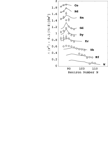
Figure 1: Observed (symbols) and calculated (lines) isotope shifts (in fm²) for isotopic chains in the rare-earth region. The quantity $0.1(74-Z)$ fm² is added to $\Delta\langle r^{2}\rangle$ for display purposes. Data are from Ref. isotope .

This value is rather reliably determined from the peaks in the isotope shifts in the spherical-deformed transitional region and reproduces the essential features of charge radii in all isotopic chains with the exception of the light Yb isotopes.

A more direct way to fix the parameter $\eta$ is from isomer shifts since this quantity is directly proportional to $\eta$. Of the few isomer shifts known in the rare-earth region, only the Gd isomer shifts have been measured with different techniques to give consistent values and these agree with the theoretical results calculated with $\eta=0.5$ fm² Zerguineun .

With the parameter $\eta$ determined from isotope and isomer shifts, one can now compute $\rho^{2}$ values in the rare-earth region using the E0 transition operator (7). The results are compared with the available data in Table 1.

Table 1: Calculated and experimental Wood99 ; Kibedi05 $\rho^{2}$ values between levels with angular momentum $J$ and initial and final energies $E_{\rm i}$ and $E_{\rm f}$ (in keV).

Isotope		Transition				$J$		$\rho^{2}\times 10^{3}$
		$E_{\rm i}$		$E_{\rm f}$				Calc		Expt
150Sm		740	$\rightarrow$	0		0		08		18 2
		1046	$\rightarrow$	334		2		18		100 40
152Sm		685	$\rightarrow$	0		0		57		51 5
		811	$\rightarrow$	122		2		45		69 6
		1023	$\rightarrow$	366		4		32		88 14
		1083	$\rightarrow$	0		0		03		0.7 4
		1083	$\rightarrow$	685		0		52		22 9
152Gd		615	$\rightarrow$	0		0		76		63 14
		931	$\rightarrow$	344		2		86		35 3
154Gd		681	$\rightarrow$	0		0		95		89 17
		815	$\rightarrow$	123		2		74		74 9
156Gd		1049	$\rightarrow$	0		0		58		42 20
		1129	$\rightarrow$	89		2		46		55 5
158Gd		1452	$\rightarrow$	0		0		34		35 12
		1517	$\rightarrow$	79		2		30		17 3
158Dy		1086	$\rightarrow$	99		2		47		27 12
160Dy		1350	$\rightarrow$	87		2		32		17 4
162Er		1171	$\rightarrow$	102		2		43		630 460
164Er		1484	$\rightarrow$	91		2		29		90 50
166Er		1460	$\rightarrow$	0		0		15		0.02 1
170Yb		1229	$\rightarrow$	0		0		36		27 5
172Yb		1405	$\rightarrow$	0		0		34		0.20 3
174Hf		900	$\rightarrow$	91		2		36		27 13
176Hf		1227	$\rightarrow$	89		2		17		52 9
178Hf		1496	$\rightarrow$	93		2		36		14 3
182W		1257	$\rightarrow$	100		2		51		3.5 3
184W		1121	$\rightarrow$	111		2		58		2.6 5

Table 1 illustrates the successes and failures of the present approach. In the Sm, Gd, and Dy isotopes, the model reproduces the correct order of magnitude of the $\rho^{2}$ values for a reasonable choice of effective charges, $e_{\rm n}=0.5e$ and $e_{\rm p}=e$. In the heavier nuclei, however, one observes some glaring discrepancies, most notably in ¹⁶⁶Er, ¹⁷²Yb, and ^182-184W. One possible reason is that the strong $\rho^{2}$ to the $\beta$-vibrational band has not yet been identified experimentally in these nuclei. This seems to be the case in ¹⁶⁶Er where recently Wimmer et al. Wimmerun measured a $\rho^{2}$ value of 127 (60) $10^{-3}$ to an excited $0^{+}$ state at 1934 keV. At present this observation is difficult to place in the systematics of the $\beta$-vibrational band in the Er isotopes and therefore a re-measurement of E0 properties seems in order before attempting a re-interpretation of these nuclei. Many $\rho^{2}$ values have been measured in ¹⁷²Yb but none of them is large leading to a confusing situation that also deserves to be revisited experimentally. Only in the W isotopes it seems certain that the observed E0 strength is consistently an order of magnitude smaller than the calculation. It is known that these nuclei are in a region of hexadecapole deformation Lee74 . This may offer a qualitative explanation of the suppression of the E0 strength, as is argued below.

From the preceding analysis the following picture emerges. Isotopic chains in the rare-earth region exhibit a spherical-to-deformed evolution which, at the phase-transitional point, is characterized by a peak in the isotope shifts. Parallel with this behavior there should be a peak in the E0 strength from the ground to an excited $0^{+}$ state. As emphasized by von Brentano et al. Brentano04 , an inescapable prediction of the $sd$-IBM is that sizable E0 strength should be observed in all deformed nuclei. We now investigate to what extent this conclusion is ‘robust’ by studying a well-known extension of $sd$-IBM through the introduction of a $g$ boson.

For a review of studies with the $sdg$-IBM we refer the reader to Devi and Kota Devi92 . A spherical-to-deformed transition occurs between the limits ${\rm U}(5)\otimes{\rm U}(9)$ and SU(3) of the $sdg$-U(15) model Devi90 . Up to a scale factor, irrelevant for the subsequent discussion, a schematic Hamiltonian, transitional between the two limits, is of the form

$$\hat{H}=(1-\zeta)(\hat{n}_{d}+\lambda\hat{n}_{g})-\frac{\zeta}{4N_{\rm b}}\hat{Q}\cdot\hat{Q},$$ (10)

where $\hat{Q}_{\mu}$ is the SU(3) quadrupole operator of the $sdg$-IBM Kota87 . The ${\rm U}(5)\otimes{\rm U}(9)$ limit is obtained for $\zeta=0$ whereas the SU(3) limit corresponds to $\zeta=1$. By varying $\zeta$ from 0 to 1 one will thus cross the critical point $\zeta_{\rm c}\approx 0.5$ at which the spherical-to-deformed transition occurs.

Analytic expressions can be derived for the matrix elements of the operators $\hat{n}_{s}$, $\hat{n}_{d}$, and $\hat{n}_{g}$ for the limiting values of $\zeta$ in the Hamiltonian (10) Zerguineun . It is instructive to compare these results to the corresponding ones in $sd$-IBM which is done in Table 2 in the classical limit $N_{\rm b}\rightarrow\infty$ of SU(3).

Table 2: Matrix elements in the classical limit of SU(3) in $sd$-IBM and $sdg$-IBM.

	$\langle 0^{+}_{1}|\hat{n}_{l}|0^{+}_{1}\rangle$						$\langle 0^{+}_{1}|\hat{n}_{l}|0^{+}_{2}\rangle$
IBM	$l=0$		$l=2$		$l=4$		$l=0$		$l=2$		$l=4$
$sd$	$\displaystyle{\frac{1}{3}N_{\rm b}}$		$\displaystyle{\frac{2}{3}N_{\rm b}}$		—		$\displaystyle{\frac{2}{3}\sqrt{\frac{N_{\rm b}}{2}}}$		$\displaystyle{-\frac{2}{3}\sqrt{\frac{N_{\rm b}}{2}}}$		—
$sdg$	$\displaystyle{\frac{1}{5}N_{\rm b}}$		$\displaystyle{\frac{4}{7}N_{\rm b}}$		$\displaystyle{\frac{8}{35}N_{\rm b}}$		$\displaystyle{\frac{2}{5}\sqrt{\frac{N_{\rm b}}{3}}}$		$\displaystyle{\frac{2}{7}\sqrt{\frac{N_{\rm b}}{3}}}$		$\displaystyle{-\frac{24}{35}\sqrt{\frac{N_{\rm b}}{3}}}$

Considering first the expectation values of $\hat{n}_{l}$ in the ground state, we note that $d$ bosons are dominant in $0^{+}_{1}$ both in $sd$- and $sdg$-IBM and that the contribution of $g$ bosons in $sdg$-IBM is small. One therefore does not expect a significant effect of the $g$ boson on the nuclear radius, and this should be even more so away from the SU(3) limit for a realistic choice of boson energies, $0<\epsilon_{d}<\epsilon_{g}$. Turning to the $\langle 0^{+}_{1}|\hat{n}_{l}|0^{+}_{2}\rangle$ matrix elements, we see from Table 2 that the matrix elements of $\hat{n}_{d}$ and $\hat{n}_{g}$ in $sdg$-IBM are of comparable size and different sign. Therefore, while changes in the nuclear radius due to the $g$ boson are expected to be small, one cannot rule out its significant impact on the $\rho^{2}(0^{+}_{\beta}\rightarrow 0^{+}_{1})$ values in deformed nuclei.

This argument can be made more quantitative by studying the spherical-to-deformed shape transition of the Hamiltonian (10). Using a numerical code Heinzeun the matrix elements of $\hat{n}_{d}$ and $\hat{n}_{g}$ can be calculated for arbitrary $\zeta$. For the ratio of boson energies we choose $\lambda=1.5$. The results are shown in Fig. 2 and compared with the matrix elements of $\hat{n}_{d}$ calculated for the U(5)-to-SU(3) transition in $sd$-IBM.

Figure 2: The matrix elements (a) $\langle 0^{+}_{1}|\hat{n}_{l}|0^{+}_{1}\rangle$ and (b) $\langle 0^{+}_{1}|\hat{n}_{l}|0^{+}_{2}\rangle^{2}$ for $l=2$ and $l=4$ in the spherical-to-deformed transition of $sd$-IBM and $sdg$-IBM. In $sd$-IBM the transition is from U(5) to SU(3) and $sdg$-IBM from ${\rm U}(5)\otimes{\rm U}(9)$ to SU(3) with $\lambda=1.5$. The number of bosons is $N_{\rm b}=8$.

Panel (a) of the figure confirms the dominance of the $d$ boson in the ground state of deformed nuclei both in $sd$- and $sdg$-IBM. Moreover, the expectation value of $\hat{n}_{d}$ varies with $\zeta$ in very much the same way in both models. In $sd$-IBM as well as in $sdg$-IBM the sharp increase in $\langle 0^{+}_{1}|\hat{n}_{d}|0^{+}_{2}\rangle^{2}$ is observed around $\zeta_{\rm c}\approx 0.5$. Up to that point there is essentially no contribution to $\rho^{2}(0^{+}_{2}\rightarrow 0^{+}_{1})$ from the $g$ boson. Consequently, all $sd$-IBM E0 results up to the phase-transitional point are not modified significantly by the $g$ boson. As can be seen from Fig. 2b, in the deformed regime this is no longer true since, in $sdg$-IBM, a sharp decrease of $\langle 0^{+}_{1}|\hat{n}_{d}|0^{+}_{2}\rangle^{2}$ occurs at $\zeta\approx 0.5$ and $\langle 0^{+}_{1}|\hat{n}_{g}|0^{+}_{2}\rangle^{2}$ rapidly increases after $\zeta\approx 0.6$ and dominates $\langle 0^{+}_{1}|\hat{n}_{d}|0^{+}_{2}\rangle^{2}$ for $\zeta\geq 0.7$.

In summary, the correlation between radii and E0 transitions has been investigated in transitional nuclei. A quantitative analysis of radii and $\rho^{2}$ values in the rare-earth nuclei seems to validate the explanation of E0 strength which is based on a geometric picture of the nucleus as advocated a long time ago Reiner61 . The proposed correlation depends on the effective charges appearing in the radius and E0 operators, assumed to be the same, and establishes a method to determine these charges empirically. The hexadecapole deformation which has only a weak effect on the nuclear radius but possibly a strong one on E0 transitions, might perturb the correlation in deformed nuclei.

We wish to thank Ani Aprahamian, Lex Dieperink, and Kris Heyde for helpful discussions. This work has been carried out in the framework of CNRS/DEF project N 19848. S.Z. thanks the Algerian Ministry of High Education and Scientific Research for financial support.

References

- (1) E.L. Church and J. Weneser, Phys. Rev. 103, 1035 (1956).
- (2) J. Kantele, Heavy Ions and Nuclear Structure, Proc. XIVth Summer School, Mikolajki, edited by B. Sikora and Z. Wilhelmi (Harwood, New York, 1984).
- (3) J.L. Wood, E.F. Zganjar, C. De Coster, and K. Heyde, Nucl. Phys. A 651, 323 (1999).
- (4) F. Iachello and A. Arima, The Interacting Boson Model (Cambridge University Press, Cambridge, 1987).
- (5) The factor is included because it is the fraction which is a measure of the quadrupole deformation. Slightly less good but still reasonable results are obtained without the factor .
- (6) A. Bohr and B.R. Mottelson, Nuclear Structure. I & II (Benjamin, New York, 1969 &1975).
- (7) J.N. Ginocchio and M.W. Kirson, Nucl. Phys. A 350, 31 (1980).
- (8) S. Zerguine et al., to be published.
- (9) J.E. García-Ramos, J.M. Arias, J. Barea, and A. Frank, Phys. Rev. C 68, 024307 (2003).
- (10) A.S. Reiner, Nucl. Phys. 27, 115 (1961).
- (11) B. Cheal et al., J. Phys. G 29, 2479 (2003); E. Otten, Treatise on Heavy-Ion Science. Volume 8, edited by D.A. Bromley (Plenum, New York, 1989); J. Frick et al., At. Data Nucl. Data Tables 60, 177 (1995); I. Angeli, At. Data Nucl. Data Tables 87, 185 (2004); W.G. Jin et al., Phys. Rev. A 49, 762 (1994).
- (12) T. Kibedi and R.H. Spear, At. Data Nucl. Data Tables 89, 77 (2005); W.D. Kulp et al., arXiv:0706.4129 [nucl-ex].
- (13) K. Wimmer et al., arXiv:0802.2514 [nucl-ex].
- (14) I.Y. Lee, J.X. Saladin, C. Baktash, J.E. Holden, and J. O’Brien, Phys. Rev. Lett. 33, 383 (1974).
- (15) P. von Brentano, V. Werner, R.F. Casten, C. Sholl, E.A. Mc Cutchan, R. Krücken, and J. Jolie, Phys. Rev. Lett. 93, 152502 (2004).
- (16) Y.D. Devi and V.K.B. Kota, Pramana J. Phys. 39, 413 (1992).
- (17) Y.D. Devi and V.K.B. Kota, Z. Phys. A 337, 15 (1990).
- (18) V.K.B. Kota, J. Van der Jeugt, H. De Meyer, and G. Vanden Berghe, J. Math. Phys. 28, 1644 (1987).
- (19) S. Heinze, Program ArbModel, University of Köln (unpublished).