Against Tachyophobia

Abstract

We examine the possible extension of the parameter space of the minimal supersymmetric extension of the Standard Model (MSSM), as expressed via the renormalization-group equations in terms of universal soft supersymmetry-breaking terms at the unification scale, to include tachyonic input scalar masses. Many models with negative masses-squared for scalars at the unification scale may be viable because the small sizes of the masses-squared allow them to change signs during the renormalization-group evolution to the electroweak scale. However, in many cases, there is, in addition to the electroweak vacuum, a much deeper high-scale vacuum located along some F- and D-flat direction in the effective potential for the MSSM. We perform a numerical search for such vacua in both the CMSSM and the NUHM. We discuss the circumstances under which the existence of such a deep charge- and color-breaking vacuum is consistent with standard cosmology. A crucial role is played by the inflation–induced scalar masses, whereas thermal effects are often irrelevant.

I Motivation

Understanding the allowed parameter space in versions of the Minimal Supersymmetric extension of the Standard Model (MSSM) with Grand Unified Theory (GUT) inspired boundary conditions is a research programme that gains motivation at the onset of the LHC. In the constrained MSSM (CMSSM), in which gaugino and scalar masses are unified at the GUT scale, and its generalizations with non-universal boundary conditions, e.g., for the Higgs scalar masses (NUHM), the identity and relic density of the lightest supersymmetric particle (LSP) place strong constraints on the parameter space cmssmwmap . For example, in models with small values of the unified scalar mass, $m_{0}$, and large values of the gaugino mass, $m_{1/2}$, the LSP is typically the lighter spartner of the $\tau$ lepton. This region of the MSSM parameter space would predict charged dark matter, and hence would be excluded if $R$-parity is conserved and the $\tilde{\tau}_{1}$ is stable. However, this corner of parameter space might be allowed if the gravitino is lighter than the $\tilde{\tau}_{1}$, and becomes the LSP gdm , as may occur in mSUGRA models vcmssm . In this case, the $\tilde{\tau}_{1}$ decays to the gravitino LSP, and is subject to important astrophysical constraints that do not exclude this region. If the gravitino is the LSP, the CMSSM parameter space may even extend to negative values of $m_{0}^{2}$ m2neg . In this paper, we argue against excluding all of this region because of unreasoning tachyophobia.

One can define an effective MSSM model by specifying its mass parameters at the weak scale. In models with relatively light squark masses, the renormalization-group equations (RGEs) for the scalar masses may then lead to $m^{2}(Q_{0})=0$, for some value of $Q_{0}$ in the range $M_{W}<Q_{0}<M_{GUT}$, with $m^{2}(Q)<0$ for $Q>Q_{0}$. This raises the question whether there is a dangerous charge- and color-breaking (CCB) vacuum . The answer to this question depends on two factors: whether there are potentially large logarithmic corrections to the potential which are not absorbed in the running of mass parameters, and whether there are significant non-renormalizable terms in the effective potential. In general these vacua, determined by minimization of the tree–level scalar potential, occur with vacuum expectation values (vevs) of order $v^{2}\sim|m^{2}|\ll Q_{0}^{2}$. However, $m^{2}(Q)<0$ and the existence of F- and D-flat directions in the MSSM leads to runaway to $v(Q)\sim Q$ for $Q>Q_{0}$, where logarithmic corrections are small. Such a CCB vacuum would exist if there were no non-renormalizable terms in the effective potential, but such terms are in general present, and their magnitudes determine where the runaway vev is stabilized and hence whether the existence and location of such a CCB vacuum can be calculated reliably. Thus, as argued in FORS , for certain parameter choices, vevs will indeed be generated with $v(Q)\sim Q$ for $Q>Q_{0}$, ensuring the existence of the CCB vacuum unless new physics between the GUT and electroweak scale is introduced. Here we will enlarge upon this idea and identify the flat directions that are primarily responsible in the CMSSM and NUHM.

However, it is possible that such CCBs could be tolerated RR , if the Universe would have fallen naturally into our false electroweak (EW) vacuum as the cosmological temperature decreased, and if the lifetime of this vacuum for tunnelling into the true CCB vacuum is much longer than the present age of the Universe. Whether the EW vacuum is in fact preferred by cosmology depends, in particular, on the scalar masses-squared generated during inflation. If these masses-squared are positive and of the order of the square of the Hubble parameter, the ‘more symmetric’ EW vacuum is favored. On the other hand, if these are negative, as in the Affleck-Dine scenario for baryogenesis AD , the Universe would remain trapped in the true CCB vacuum FORSS .

The present article delineates regions of parameter space for which high-scale CCB vacua are present. We study both the CMSSM and less constrained models with non-universal Higgs masses (NUHM) nonu ; nuhm . For each choice of GUT-scale parameters, we follow the analysis of GKM for determining the set of problematic flat directions and the lowest order of GUT- or Planck-scale non-renormalizable operators whose appearance might lift the flat direction. The existence of CCB vacua will depend on both the order of the non-renormalizable operator and the fundamental scale associated with it. In the case of the CMSSM, there are wedges of parameter space with $m^{2}_{0}<0$ where no MSSM sfermion is tachyonic at the EW scale. However, these regions generally have calculable CCB vacua, assuming that the mass scale $M_{*}$ in the non-renormalizable interaction that stabilizes the high-scale vacuum is greater than or equal to $M_{GUT}$. Such regions would be acceptable in suitable cosmological scenarios that populate exclusively the EW vacuum. Similar questionable tachyonic regions occur also in the NUHM, even if $m^{2}_{0}>0$, due to the (independent) squared masses for Higgses being negative. However, we emphasize again that these regions would be acceptable in cosmological scenarios that avoid populating high-scale vacua: one should not be unreasoningly tachyophobic.

II CCBs along Flat Directions in the MSSM

The tree-level scalar potential can be written schematically (including soft supersymmetry-breaking contributions) as

$$V=\frac{1}{2}\tilde{m}^{2}(Q)\phi^{2}+\frac{1}{4}\lambda(Q)\phi^{4},$$ (1)

where, for simplicity, we have neglected cubic terms, and $\lambda$ may vanish along some directions in $\phi$ space. We assume as well that some set of soft supersymmetry-breaking scalar masses have $\tilde{m}^{2}(Q)<0$ for $Q$ above some scale $Q_{0}$, for a particular choice of GUT-scale parameters in the CMSSM or NUHM. Along a generic direction in field space, with $\lambda(Q)\sim g^{4}$ where $g$ is some gauge coupling, minimization of the tree-level potential yields a vev at $\phi=v(Q)=[-\tilde{m}^{2}(Q)/\lambda(Q)]^{1/2}$ which is of similar order to the supersymmetry-breaking scale, $m_{3/2}$. However, one-loop corrections to the potential will have the form $\Delta V\sim\tilde{m}^{2}(Q)v(Q)^{2}\ln[v(Q)^{2}/Q^{2}]$ and, for $v\ll Q_{0}$, the large logarithms may reduce significantly the reliability of the CCB vacuum calculation.

On the other hand, the appearance of negative mass-squared $\tilde{m}^{2}$ would have important implications for the moduli $\eta$ of the flat directions in the MSSM where $\lambda=0$, since the tree-level solution yields a runaway vev. However, we expect high-scale non-renomalizable operators to regulate the runaway behaviour in such a case. In the presence of a non-renormalizable superpotential $W_{\text{NR}}$ of degree $n$ (see Appendix A), the effective potential becomes

$$V=\tilde{m}^{2}|\eta|^{2}+\frac{|u|^{2}}{M_{*}^{2(n-3)}}|\eta|^{2(n-1)}$$ (2)

and the runaway direction for the modulus $\eta$ is stabilized. In (2), $u$ is an ${{\cal O}(1)}$ dimensionless coupling constant and $M_{*}$ is the cutoff scale associated with the dynamics that generates $W_{\text{NR}}$. Depending on the circumstance, it could be between the unification scale and the Planck scale. The modulus $\eta$ then acquires a vev whose order of magnitude is given by:

$$v\equiv\left[-\tilde{m}^{2}M_{*}^{2(n-3)}\right]^{\frac{1}{2(n-2)}}\quad\left(\sim|\eta|\right).$$ (3)

General properties of flat directions and the operators which lift them are found in Appendix A, and examples of specific MSSM flat directions are given in Appendix B.

The one-loop correction to the scalar potential can be written as

$$\Delta V_{\text{1-loop}}=\frac{N}{64\pi^{2}}g^{2}v^{2}\tilde{m}_{\text{avg}}^{2}\ln\frac{g^{2}v^{2}}{Q^{2}},$$ (4)

where $N$ is the number of multiplets that get masses at the scale $m=gv$. The cancellation between boson and fermion loops has been taken into account, as is apparent from the factor $\tilde{m}_{\text{avg}}^{2}$. This is an average soft supersymmetry-breaking mass-squared, determined from the one-loop contributions of the $N$ states.

If $v$ is small, the overall loop correction can be large relative to the tree-level potential (2), which satisfies $V\sim{{\cal O}(\tilde{m}^{2}v^{2})}$ near the minimum, rendering the tree-level analysis unreliable. We introduce a parameter ${\epsilon}$ that represents the boundary where this large-logarithm problem occurs:

$$v\mathrel{\hbox to0.0pt{\raise 2.15277pt\hbox{$<$}\hss}{\lower 2.15277pt\hbox{$\sim$}}}{\epsilon}Q\Rightarrow\text{unreliable},\quad v\mathrel{\hbox to0.0pt{\raise 2.15277pt\hbox{$>$}\hss}{\lower 2.15277pt\hbox{$\sim$}}}{\epsilon}Q\Rightarrow\text{reliable}.$$ (5)

Since $v$ shuts off at low $Q$ in the models we consider, it is possible in principle that the tree-level analysis may never be reliable. We have nothing to say about such models in this article, except that they are not excluded by our analysis. On the other hand, when we find a vev $v$ and there is a regime of $Q$ for which this tree-level result is reliable, a vacuum state really exists at some large value of the modulus $\eta$. The existence of this deep vacuum at large field values—generally color or charge breaking (CCB)—has cosmological implications, which we discuss below. To determine the parameter ${\epsilon}$, we note that the loop correction (4) is comparable to the tree term $\tilde{m}^{2}v^{2}$ when:

$$\frac{N}{64\pi^{2}}g^{2}\ln\frac{v^{2}}{Q^{2}}\sim-1\quad\Rightarrow\quad{\epsilon}=\exp(-32\pi^{2}/Ng^{2}).$$ (6)

When $v\geq{\epsilon}Q$, we can reliably state that at least two vacua exist: the electroweak (good) vacuum and the high-scale (bad) one.

Now a word on numbers: in (6), we should take $1/10<g^{2}<1/2$, corresponding to the running constants between the EW and GUT scales. The number $N$ depends on the flat direction, but would typically range between ${{\cal O}(10)}$ and ${{\cal O}(100)}$. For the larger value of $N$, we have ${\epsilon}\mathrel{\hbox to0.0pt{\raise 2.15277pt\hbox{$<$}\hss}{\lower 2.15277pt\hbox{$\sim$}}}{{\cal O}(10^{-3})}$; moreover, ${\epsilon}$ falls exponentially as $N$ decreases, so it is generically much smaller than $10^{-3}$. In other words, the loop factor suppression $g^{2}/64\pi^{2}$ means that the logarithmic enhancement must be quite large before the tree-level analysis becomes unreliable. As a consequence, the RG-improved tree-level analysis is generally a reliable indicator of the high-scale vacuum.

As an example, consider the $LLe^{c}$ flat directions in the MSSM. Eleven chiral multiplets participate in the mass matrix once renormalizable superpotential terms are accounted for, namely $e_{i},\nu_{i},e_{i}^{c},H_{d}^{0},H_{d}^{-}$. The moduli space is ${\bf C}^{3}$ once D- and F-flatness constraints are taken into account GKM . Thus eight chiral multiplets get ${{\cal O}(v)}$ masses, although in some cases they are suppressed by very small Yukawa couplings $y_{i}^{e}$, corresponding to D-moduli whose flatness is lifted by the renormalizable superpotential . Furthermore, $SU(2)\times U(1)$ gauge multiplets get ${{\cal O}(gv)}$ masses. Each chiral multiplet contributes 2 to $N$, because it includes a complex scalar and a Weyl fermion. A similar contribution comes from each of the four vector multiplets contained in $SU(2)\times U(1)$. Thus $N=2(8+4)=24$. Even if we assume the GUT-scale value $g^{2}=1/2$, we already get ${\epsilon}\sim 4\times 10^{-12}$. In actuality, for many of the masses we should use $(y_{i}^{e})^{2}\ll g^{2}$ and ${\epsilon}$ is even much smaller still. The result is that we trust the tree-level analysis for practically all $v/Q$: it is a robust result that we have at least these two vacua, and the cosmological arguments apply.

Fig. 1 represents schematically several generic cases for the possible variation with $Q$ of the vev $v(Q)$. For each of the curves #1 – #4, $v(Q)\neq 0$ at large $Q$, but $v(Q)\to 0$ at small $Q$. In each of the cases #1 – #3, the condition (5) is satisfied over some range of $Q$ and hence, according to the arguments presented above, the existence of a high-scale vacuum can be predicted reliably in each of these cases. These are representative of what happens in much of the parameter space that we study below in specific CMSSM and NUHM scenarios. On the other hand, when we consider curve #4 in Fig. 1, we see that, over the entire range of $Q$, the tree-level prediction cannot be trusted, owing to the persistence of large logarithms. For this reason, we exercise caution and choose not to apply the cosmological constraint in such a case. In some specific cases, a one- or two-loop analysis might be reliable, and the possibility of a high-scale (bad) minimum could be examined in more detail. However, studies of such possibilities lie beyond the scope of this work, where we restrict ourselves conservatively to the criterion (5).

Figure 1: Curves of the flat direction vev $v=v(Q)$ (solid) versus various constraint curves (dashed). In regions where $v(Q)$ lies above the dashed lines, the tree-level effective potential is a reliable indicator for the existence of a high-scale (bad) vacuum, according to the criterion (5).

III The Cosmological Constraint

Having established the criteria for determining the existence of a high-scale vacuum (which we apply to specific CMSSM and NUHM models in the following two sections), we now turn our attention to the cosmology of models with high-scale vacua, asking how problematic their existence may be. Such a global CCB vacuum with $v\sim Q\gg M_{W}$ is separated from the local charge- and color-conserving minimum at the origin (or the EW scale if the Higgses are the scalars in question) by a potential barrier. As argued in RR , this model remains perfectly acceptable if the Universe is trapped in the local minimum near or at the origin, as the timescale for producing a bubble of lower high-scale vacuum is generally much longer than the age of the Universe.

However, in models with negative $m_{0}^{2}(M_{\rm GUT})$, there are many such vacua corresponding to different flat directions, and each has a larger domain of attraction than that of the EW vacuum. Thus, for arbitrary initial conditions, the system is overwhelmingly likely to end up in one of the ‘bad’ vacua. However, this question must be analyzed in some appropriate cosmological setting, which introduces two extra ingredients affecting the shape of the effective potential: inflation and thermal effects. During inflation, supersymmetry is broken by the vacuum energy, which results in an extra contribution to the soft scalar masses, of the general form drt

$$\Delta m^{2}=cH^{2}\;,$$ (7)

where $H$ is the Hubble expansion rate during the inflationary epoch. The dynamics of the flat directions depend crucially on the sign of $c$, which is model-dependent. For a minimal Kähler potential, $c=3$. On the other hand, for a no-scale Kähler potential, the induced scalar masses are zero at the tree level and loop corrections generate $c<0$ for flat directions not involving the stop gmo .

We now consider different possibilities for the coefficient $c$, considering first the possibility $c>0$. We assume also that the initial value of the flat-direction field $\phi$ is $10^{17}$ GeV, in which case $V(\phi)\ll V_{\rm inflaton}$, and the evolution of $\phi$ does not affect the Hubble constant significantly until the late stage when $H\sim m_{3/2}$. In this case, $\phi$ obeys the equation of motion

$$\ddot{\phi}+3H\dot{\phi}+V^{\prime}(\phi)=0\;,$$ (8)

where $H$ is a slowly-varying function of time that can be described by an adiabatic approximation. For our purposes, $V^{\prime}$ can be approximated by $cH^{2}\phi$ until $H$ becomes comparable to $m_{3/2}$. The effect of the non–renormalizable term in $V(\phi)$ is less significant. The general solution of (8) is

$$\phi(t)=C_{1}\exp\left[{1\over 2}H(-3+\sqrt{9-4c})~{}t\right]+C_{2}\exp\left[{1\over 2}H(-3-\sqrt{9-4c})~{}t\right]\;,$$ (9)

where $C_{1,2}$ are determined by the initial conditions.

We consider first the $classical$ evolution. For $c={\cal O}(1)$, the magnitude of $\phi$ scales as $\phi(t)\sim\exp[-{\cal O}(1)Ht]$. Thus, within 5-10 Hubble times, $\phi$ will be of order $H$ even if its initial value was very large  and, within the next $\sim$30 Hubble times, $\phi$ will be of the electroweak scale.

We next take into account the de Sitter quantum fluctuations, which play an important role in the dynamics of flat directions FORSS . For a scalar field of mass $\sim H$ lin2 ,

$$\langle\phi^{2}\rangle\sim H^{2}.$$ (10)

It is then clear that at large $\phi$, the classical damping dominates and when $\phi$ becomes comparable to $H$, these quantum fluctuations are as important as the classical evolution. From that moment on, $\phi$ undergoes random oscillations of order $H$ per Hubble time plus classical damping which decreases its magnitude by a factor ${\cal O}(1)$ per Hubble time. As $H(t)$ decreases, so does the amplitude of random oscillations about the origin. At the time when the soft term $m^{2}_{0}$ becomes relevant (which is after the ‘inflaton oscillation’ era), the amplitude of oscillations is ${\cal O}(m_{3/2})$. The field settles at the origin and the quantum oscillations are too small to reach the barrier separating the two minima, which is further than ${\cal O}(m_{3/2})$ away from the origin. Therefore, the presence of a deep CCB minimum would not be problematic for $c\sim 1$.

However, these conclusions do not in general apply for small positive $c$: $0<c\ll 1$, which is a borderline case. First, the classical evolution is slow and, secondly, the amplitude of quantum oscillations is larger: $\langle\phi^{2}\rangle\simeq{3H^{2}/(8\pi^{2}c)}.$ Whether the field settles at the origin at the end of inflation depends on further specifics of the inflationary model as well as the magnitude of $c$.

For $c\leq 0$ (see drt ), the minimum of the potential during (as well as after) inflation is at large $\phi$. Classical evolution will drive $\phi$ towards this minimum, whose position is a slowly-evolving function of time. At $H\sim{m_{3/2}}$, the field freezes at the CCB minimum, and the quantum fluctuations do not play any significant role. It is important to note also that thermal effects are irrelevant at large $\phi$ and cannot destabilize the CCB minimum. This is because all the fields $\phi$ couple and receive masses of order $\phi$ (multiplied by the gauge or Yukawa couplings). Thus they are heavy and cannot be thermalized. Consequently, no thermal mass term $T^{2}\phi^{2}$ is generated by thermal loops .

We thus conclude that, for $c\leq 0$, the presence of deep CCB minima is ruled out by cosmological considerations. This applies in particular to models with the Heisenberg symmetry BG , including no-scale models of supergravity ns . Furthermore, this precludes the possibility of the Affleck-Dine (AD) mechanism for baryogenesis AD , which requires negative $c$ drt . Concretely, this applies to the cases #1 – #3 of Fig. 1, in which the existence of such a bad high-scale CCB can be predicted reliably. On the other hand, even these cases would not be excluded for positive $c\sim 1$, and possibly also for small positive $c$.

We remark finally that we have neglected the trilinear soft supersymmetry-breaking $A$-terms in the above considerations. In general, one expects $A$-terms of order $H$ to be generated during inflation. If their magnitude is a few times larger than $H$, an additional local minimum at large $\phi$ appears even for positive $c\sim 1$. Given a large initial value of $\phi$, the field will evolve to this minimum and remain there after inflation. Thus, deep CCB vacua can be problematic even for $c\sim 1$, if the $A$-terms are sufficiently large.

In what follows, we will examine specific CMSSM and NUHM parameter sets for which $\tilde{m}^{2}<0$ at some high renormalization scale, with the aim of elucidating whether one should worry about them.

IV Tachyons in the CMSSM

We begin by considering the parameter space of the CMSSM, in which all gaugino masses are unified at a common scale (where gauge-coupling unification occurs) with the common value $m_{1/2}$. Similarly, all soft scalar masses are unified at the same renormalization scale with a common value $m_{0}$, as are the trilinear terms with a common value $A_{0}$. The remaining free parameters are the ratio of the two Higgs vevs, parametrized by $\tan\beta$, and the sign of the $\mu$ parameter.

For each choice of these four input parameters (plus the sign of $\mu$), the low-energy spectrum can be determined and compared with phenomenological and cosmological constraints. In Fig. 2, we show the $(m_{1/2},m_{0})$ plane for two fixed values of $\tan\beta$, both for $\mu>0$ and $A_{0}=0$. The sign displayed on the vertical axis is actually the sign of $m_{0}^{2}$, so what is displayed is $m_{0}^{2}/|m_{0}|$, strictly speaking. In panel (a), we have fixed $\tan\beta=10$ and, for $m_{0}^{2}>0$, we see results common in many CMSSM studies cmssmwmap . The dark (brown) shaded region corresponds to the region for which the stau is the LSP and as such this region is normally excluded unless the gravitino is in fact the LSP . The medium (green) shaded region, at low $m_{1/2}$ is excluded by the constraint arising from the branching ratio of $b\to s\gamma$. The vertical dashed line is the chargino mass contour at 104 GeV, and the nearly vertical dot-dashed line is the Higgs mass contour at 114 GeV, as obtained using FeynHiggs FeynHiggs . Only regions to the right of these lines are allowed by LEP. The pink band bordered by black solid curves is the region where supersymmetric corrections to the Standard-Model calculation of $(g-2)_{\mu}$ match the experimental measurement of $(g-2)_{\mu}$ within 2-$\sigma$ uncertainties (between the dashed curves agreement occurs at the 1-$\sigma$ level). Finally, in the (turquoise) shaded region that tracks the stau LSP boundary at large $m_{1/2}$, the relic density of the lightest neutralino would lie in the range of the cold dark matter density determined by WMAP and other observations wmap , if this neutralino were the LSP.

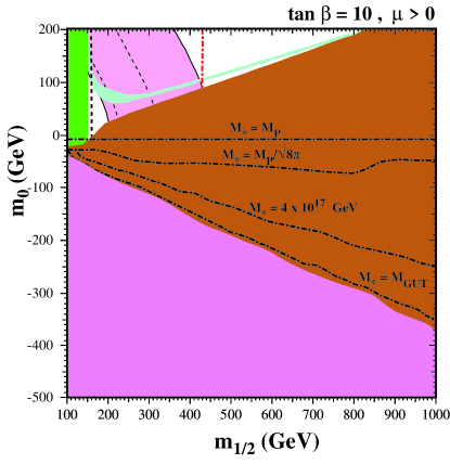
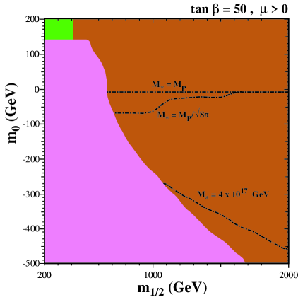
(a)	(b)

Figure 2: Portions of the CMSSM $(m_{1/2},m_{0})$ planes for (a) $\tan\beta=10$ and (b) $\tan\beta=50$. The notations are described in the text. The lower pink region is excluded because the lighter stau would be tachyonic at the EW scale. The regions below the dash-dotted curves have problematic high-scale tachyons for the indicated values of $M_{*}$ if $\epsilon=1$, while for ${\epsilon}\mathrel{\hbox to0.0pt{\raise 2.15277pt\hbox{$<$}\hss}{\lower 2.15277pt\hbox{$\sim$}}}10^{-3}$ all regions with $m_{0}^{2}<0$ are excluded.

Also shown in Fig. 2 (a) is a large (pink) shaded region at low $m_{1/2}$ and negative $m_{0}^{2}$ where one of the sfermions is tachyonic at the electroweak scale. This region is also excluded. Of particular interest to us here is the region where $m_{0}^{2}<0$ but the shading indicates that the lighter stau is the lightest spartner of a Standard Model particle but is not tachyonic at the electroweak scale: we repeat that parts of this region may in principle be viable m2neg if the gravitino is in fact the LSP. We perform our scan of the parameter space in this region looking for flat directions which could lead to a bad high-scale minimum of the potential.

According to the analysis of GKM , the $QQuue$ flat direction is not fully lifted until degree $n=9$, so from Eq. (3) we see that $v$ along this direction is quite close to the non-renormalizable mass scale $M_{*}$. The dot-dashed curves in Fig. 2 labeled by $M_{*}$ demarcate regions for which we find solutions to $v(Q)=Q$: for a given value of $M_{*}$, all regions below the corresponding curve admit solutions to $v(Q)=Q$. Thus, below the curves we find a bad CCB vacuum, that might invalidate the corresponding choice of parameters, subject to the cosmological considerations discussed in the previous Section. When $M_{*}=M_{P}$, all regions with $m_{0}^{2}<0$ have this problem. Because all of the scalars have $\tilde{m}^{2}_{i}<0$ at high enough scale when $m_{0}^{2}<0$, this flat direction always has a reliable bad CCB minimum when we take ${\epsilon}\mathrel{\hbox to0.0pt{\raise 2.15277pt\hbox{$<$}\hss}{\lower 2.15277pt\hbox{$\sim$}}}10^{-3}$, for all $M_{*}\geq M_{GUT}$. Thus all CMSSM models with $m_{0}^{2}<0$ and ${\epsilon}\mathrel{\hbox to0.0pt{\raise 2.15277pt\hbox{$<$}\hss}{\lower 2.15277pt\hbox{$\sim$}}}10^{-3}$ are problematic according to our analysis.

In panel (b) of Figure 2, we show the analogous parameter plane when $\tan\beta=50$, $\mu>0$ and $A_{0}=0$. The part of the $(m_{1/2},m_{0})$ plane shown is dominated by regions where the stau is the lightest sparticle apart from the gravitino (shaded dark brown) and where the stau is tachyonic at the EW scale (shaded pink). The standard CMSSM phenomenologically and cosmologically acceptable regions occur at $m_{1/2}>200$ GeV, and so are not visible in the part of the $(m_{1/2},m_{0})$ plane displayed. The wedge-shaped brown region with $m_{0}^{2}\leq 0$ has a calculable high-scale CCB minimum, as was the case $\tan\beta=10$. For this reason, we do not display planes with intermediate choices of $\tan\beta$. We have also scanned the CMSSM planes with $A_{0}\neq 0$, and the results are qualitatively similar to those shown here.

To summarize, because in practice ${\epsilon}\mathrel{\hbox to0.0pt{\raise 2.15277pt\hbox{$<$}\hss}{\lower 2.15277pt\hbox{$\sim$}}}10^{-3}$ for any possible flat direction, and more especially for the $QQuue$ one, the CMSSM with $m_{0}^{2}<0$ always has a bad CCB vacuum. However, this may not be populated, when cosmological considerations are taken into account.

V Tachyons in the NUHM

One alternative to the CMSSM is the NUHM, where the scalar partners of the quarks and leptons still unify at $M_{GUT}$, but the soft supersymmetry-breaking scalar masses associated with the two Higgs doublets do not. This class of models has, effectively, two additional free parameters relative to the CMSSM. These are often chosen to be the weak-scale values of $\mu$ and the Higgs pseudoscalar mass, $m_{A}$. Whilst it is certainly possible within the context of the NUHM to choose $m_{0}^{2}<0$ (leading to the same difficulty with the $QQuue$ flat direction as in the CMSSM), problems with CCB can already occur for certain choices of $\mu$ and $m_{A}$ even when $m_{0}^{2}>0$. This is because, when the weak scale $|\mu|$ is large, typically one or both of the Higgs squared masses $m_{1,2}^{2}=\mu^{2}+\tilde{m}^{2}_{1,2}$ is negative at the GUT scale, a problem that is accentuated at small $m_{A}$. In this case, the squark and slepton masses-squared remain positive throughout the RGE evolution, avoiding the $QQuue$ flat direction problem, and vevs $v\ll Q$ for all $Q$ may develop along the $H_{1}H_{2}$ flat direction, because this is lifted by a lower-order non-renormalizable term ($n=4$). As a consequence, a larger fraction of the parameter space is allowed.

At scales $Q$ not too far above the EW scale, one begins to see the EW vacuum. The negative masses-squared of MSSM Higgses can lead to unacceptable vacua with CCB also at this low scale. We do not include the details of such low-scale CCB vacua in the analysis, as this would require a much more careful treatment of loop corrections and contributions from all soft supersymmetry-breaking operators. For this reason, we terminate the NUHM analysis at $Q=10$ TeV in our numerical studies.

In Fig. 3, we show examples of $(\mu,m_{A})$ planes in the NUHM for fixed $m_{1/2}=300$ GeV, $m_{0}=100$ GeV, and $A_{0}=0$ with $\tan\beta=10$ (panels a, c and e) and $\tan\beta=50$ (panels b, d and f). We use the same shadings as used for the CMSSM to denote regions excluded by $b\to s\gamma$ (shaded medium (green)), which excludes much of the parameter space at $\mu<0$, and a region in which the lighter stau would be the lightest spartner of a Standard Model particle (shaded dark (brown)). This includes two areas with relatively small $\mu$ and $m_{A}$, for $\tan\beta=10$, and most of the left side of the plane. for $\tan\beta=50$. New to this figure are regions shaded dark (blue) for which the sneutrino is the lightest spartner of a Standard Model particle, that are seen at large $\mu$ and $m_{A}$, for $\tan\beta=10$, and in the upper right of the planes, for $\tan\beta=50$. At least parts of the regions with a light stau or sneutrino could be allowed if the gravitino is the LSP. Once again, the dashed vertical lines at small $\mu$ show the 104 GeV chargino mass contour. The thin blue lines show the contour where $m_{A}=2m_{\chi}$ and the regions of good neutralino relic density near these lines correspond to the rapid-annihilation funnel region familiar from the CMSSM at large $\tan\beta$. Other strips with an acceptable neutralino LSP relic density appear in the stau and sneutrino coannihilation regions, running parallel to boundaries of the brown and blue regions, and in a ‘crossover’ strip close to the chargino exclusion, where the neutralino is a mixed gaugino/higgsino state.

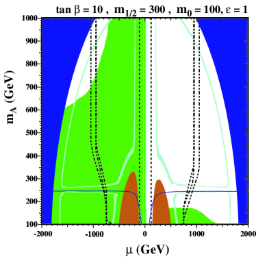
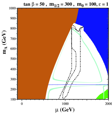
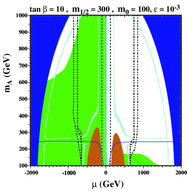
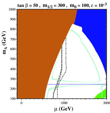
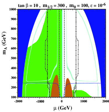
Figure 3: Portions of the NUHM $(\mu,m_{A})$ planes for for $m_{1/2}=300$ GeV, $m_{0}=100$ GeV, $A_{0}=0$ and (a, c, e) $\tan\beta=10$, (b, d, f) $\tan\beta=50$. The notations are described in the text. The regions outside the inner dash-dotted curves have problematic high-scale tachyons for higher values of $M_{*}$.

We show in each panel of Fig. 3 three dot-dashed contours with differing $M_{*}$. The inner curves (with the lowest values of $|\mu|$) correspond to $M_{*}=M_{P}$, whereas the middle and outer curves correspond to $M_{*}=M_{P}/\sqrt{8\pi}$ and $M_{GUT}$, respectively. The areas outside these contours may be problematic, depending on the cosmological scenario, as discussed previously. In panel (a) of Fig. 3, we have chosen $\epsilon=1$ and $\tan\beta=10$. The problematic region is when $|\mu|\mathrel{\hbox to0.0pt{\raise 2.15277pt\hbox{$>$}\hss}{\lower 2.15277pt\hbox{$\sim$}}}1000$ GeV, reducing to $|\mu|\mathrel{\hbox to0.0pt{\raise 2.15277pt\hbox{$>$}\hss}{\lower 2.15277pt\hbox{$\sim$}}}750$ GeV for small $m_{A}$. When $\epsilon$ is decreased to $10^{-3}$ (panel c) and $10^{-6}$ (panel e), the problematic regions extend down to smaller values of $|\mu|$, reaching as low as $\sim 550$ GeV for $\epsilon=10^{-6}$ and small $m_{A}$, essentially independent of $M_{*}$.

The most immediately noticeable features of the $(\mu,m_{A})$ planes for $\tan\beta=50$, shown in panels (b), (d) and (f) of Fig. 3, are the greater extent of the stau LSP region when $\mu\mathrel{\hbox to0.0pt{\raise 2.15277pt\hbox{$<$}\hss}{\lower 2.15277pt\hbox{$\sim$}}}1000$ GeV, and the the greater extent of the sneutrino LSP region when $\mu\mathrel{\hbox to0.0pt{\raise 2.15277pt\hbox{$>$}\hss}{\lower 2.15277pt\hbox{$\sim$}}}1000$ GeV. In between, the problematic tachyonic regions depend more sensitively on the value of $M_{*}$ than was the case for $\tan\beta=10$, and also vary more as $\epsilon$ is reduced. Once again, it is the regions of large $\mu$ that are problematic.

Whereas in the CMSSM case the stau was always lighter than the lightest neutralino in the tachyonic region, so that it could be cosmologically acceptable only if the gravitino were the LSP, in the NUHM case the tachyonic region also includes parts of the WMAP strips where the LSP is the neutralino and it has an acceptable relic density. The crossover strip, the stau coannihilation region and parts of the snu coannihilation strip and parts of the rapid-anihilation funnel with an acceptable neutralino relic density are all in the non-tachyonic parts of the $(\mu,m_{A})$ planes for $\tan\beta=10$. These regions also have acceptable $b\to s\gamma$ for $\mu>0$. In the case of $\tan\beta=50$, parts of the stau coannihilation strip and the rapid-annihilation funnel are again tachyon-free. We emphasize yet again that the tachyonic regions at larger $|\mu|$ are not necessarily excluded: that would depend on the cosmological scenario and whether it avoids the high-scale vacuum in the early Universe.

In Fig. 4, we show more examples of $(\mu,m_{A})$ planes, this time with $m_{1/2}=500$ GeV, $m_{0}=300$ GeV, and $A_{0}=0$. We see that there are regions at larger $m_{A}$, particularly for $\mu>0$, where the LEP Higgs constraint is respected. As in Fig. 3, the problematic tachyonic regions extend to smaller $|\mu|$ as $m_{A}$ decreases, and as $\epsilon$ decreases from 1 to $10^{-6}$. The potential tachyonic problem is restricted essentially to $|\mu|\mathrel{\hbox to0.0pt{\raise 2.15277pt\hbox{$>$}\hss}{\lower 2.15277pt\hbox{$\sim$}}}1000$ GeV.

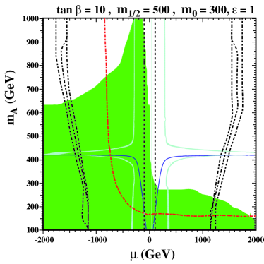
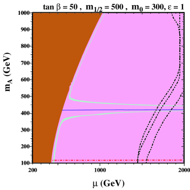
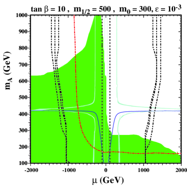
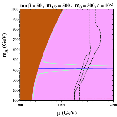
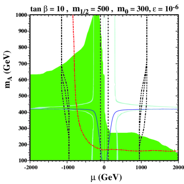
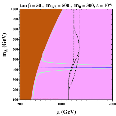
Figure 4: Portions of the NUHM $(\mu,m_{A})$ planes for for $m_{1/2}=500$ GeV, $m_{0}=300$ GeV, $A_{0}=0$ and (a, c, e) $\tan\beta=10$, (b, d, f) $\tan\beta=50$. The notations are described in the text. The regions outside the inner dash-dotted curves have problematic high-scale tachyons for higher values of $M_{*}$.

Turning to panels (b), (d) and (f) in Fig. 4, for $\tan\beta=50$, we seethat the stau LSP region extends to between $\mu\sim 400$ GeV (for small $m_{A}$) and $\mu\sim 1000$ GeV (for large $m_{A}$). The problematic tachyon region is now only at larger $\mu$, varying between a range $>2000$ GeV for $\epsilon=1$ and large $m_{A}$ to $\sim 1150$ GeV for $\epsilon=10^{-6}$ and small $m_{A}$. In all cases, the portion of the WMAP strip where the relic neutralino density is controlled by stau coannihilation is in the safe region, as well as a portion of the rapid-annihilation funnel where $m_{\chi}\sim m_{A}/2$. Whether the other regions are acceptable would depend on the cosmological scenario. Note that the entire regions shown in panels (b), (d) and (f) are favoured by $g_{\mu}-2$.

Comparing Figs. 3 and 4, we see (unsurprisingly) that the problematic tachyonic NUHM regions grow as $m_{0}$ decreases. As we noted above, it is also possible to consider $m_{0}^{2}<0$ in the NUHM. For example, For $m_{1/2}=300$ GeV and $m_{0}^{2}/\sqrt{|m_{0}^{2}|}$ = -100 GeV, with $M_{*}=M_{GUT}$ and $\epsilon=1$, CCB vacua appear at high scale when $|\mu|>1000$ GeV for $m_{A}\mathrel{\hbox to0.0pt{\raise 2.15277pt\hbox{$>$}\hss}{\lower 2.15277pt\hbox{$\sim$}}}800$ GeV and $|\mu|>1500$ GeV for lower $m_{A}$. When $\epsilon=10^{-3}$ for the same case, the entire plane is problematic. Similarly, when $M_{*}=M_{P}$ for any value of $\epsilon$, the entire plane is problematic.

VI Summary

We have discussed in this paper the constraints that are imposed on supersymmetric models by the presence of the Universe in our familiar EW vacuum. We have argued that models with tachyonic spin-zero fields at some high input scale are not necessarily excluded. The renormalization-group evolution of tachyonic masses to low scales may change their signs, in which case the standard EW vacuum would be a local minimum of the effective potential. However, in addition to this vacuum, there may be a much deeper high-scale vacuum located along some F- and D-flat direction in the effective potential, with field values fixed by some higher-order non-renormalizable interaction. We discuss the circumstances under which the existence and location of such a high-scale vacuum can be calculated reliably.

Such high-scale vacua usually break both color and charge conservation. In general, the lifetime for decay of the EW vacuum to this unacceptable lower minimum of the effective potential is much longer than the age of the Universe, so future decay into such a vacuum is not of immediate concern. A more relevant question is whether the Universe would have fallen into such a vacuum during its past history. This depends whether the effective scalar masses-squared acquired large positive or negative contributions $\propto H^{2}$ during inflation. If these contributions were ${\cal O}(1)$ and positive, only the EW vacuum would be populated. On the other hand if these contributions were negative (and possibly if they were positive but small), the high-scale vacuum would be populated.

We have then explored the conditions under which the CMSSM or the NUHM (with its two extra parameters) has a calculable high-scale vacuum. If these conditions are not satisfied, there is no reason to be tachyophobic. Even if these conditions are satisfied, and there is a calculable high-scale vacuum, whether it is catastrophic or not depends on early cosmology, and there is still no need to be tachyophobic.

Unreasoning tachyophobia is never justified: one must examine rationally whether any specific tachyonic spin-zero field is dangerous, depending on the evolution of the Universe within one’s favoured cosmological scenario.

Appendix A Generalities

Here we give a concise review of the well-known nature of the flat directions that will be considered. This Appendix is included to serve as a reminder and to set our notation.

We begin our discussion by ignoring the superpotential and soft terms, which are included later. We assume complex scalar fields $\phi_{i}$ with a canonical Kähler potential, with vevs denoted by $v_{i}$. We take $v_{i}$ to correspond to a supersymmetric vacuum, $D^{a}=0$, in the standard notation. Viewed as a vector space, the $v_{i}$ are the null vectors of the (hermitian) mass-squared matrix:

$$\sum_{k}\bar{v}_{k}M_{k\bar{\ell}}^{2}=\sum_{k,a}g_{a}^{2}\frac{{\partial}D^{a}}{{\partial}v_{k}}\frac{{\partial}D^{a}}{{\partial}\bar{v}_{\bar{\ell}}}\bar{v}_{k}=\sum_{a}g_{a}^{2}D^{a}\frac{{\partial}D^{a}}{{\partial}\bar{v}_{\bar{\ell}}}=0.$$ (11)

Correspondingly, there exists a projection operator into this null space:

$$P_{ij}=\frac{v_{i}\bar{v}_{j}}{\sum_{k}|v_{k}|^{2}}.$$ (12)

which may be used to construct the modulus field $\eta$, which is the scalar field tangential to the null space defined by $P$:

$$\eta=\sum_{j}\frac{\bar{v}_{j}}{\sqrt{\sum_{k}|v_{k}|^{2}}}\phi_{j}.$$ (13)

In addition, there are the other modes $\chi_{\alpha}$, that are orthogonal to $\eta$ in the space of the $\phi_{i}$, i.e.:

$$\chi_{\alpha}=\sum_{i}\bar{\theta}_{i}^{\alpha}\phi_{i}:\quad\sum_{i}\theta_{i}^{\alpha}\bar{v}_{i}=0,\quad\sum_{i}\bar{\theta}_{i}^{\alpha}\theta_{i}^{\beta}=\delta^{\alpha\beta}.$$ (14)

We now consider the effect of the soft masses on the modulus field $\eta$. When the change of variables (13) is made, we obtain:

$$V_{\text{soft}}\ni\sum_{i}\tilde{m}^{2}_{i}|\phi_{i}|^{2}\ni\frac{\sum_{i}|v_{i}|^{2}\tilde{m}^{2}_{i}}{\sum_{k}|v_{k}|^{2}}|\eta|^{2}\equiv\tilde{m}^{2}|\eta|^{2}.$$ (15)

In the case of a flat direction characterized by a single monomial

$$\Phi=\prod_{i}\phi_{i}^{n_{i}},$$ (16)

the D-flatness constraint

$$\bar{\phi}_{i}=\frac{{\partial}\Phi}{{\partial}\phi_{i}}\cdot\text{const}\quad\forall\quad i$$ (17)

yields:

$$|v_{i}|^{2}=n_{i}\cdot\text{const}\quad\forall\quad i.$$ (18)

It follows that in this case the modulus soft mass-squared appearing in (15) is:

$$\tilde{m}^{2}=\frac{\sum_{i}n_{i}\tilde{m}^{2}_{i}}{\sum_{k}n_{k}},$$ (19)

where we see that the weights are nothing but the powers in the monomial. Because we specialize to the case of monomial flat directions (16) in our study, we use (19) to determine the soft masses of moduli. The cases that we are interested in are those with

$$\tilde{m}^{2}(Q)<0,$$ (20)

where $Q$ is the running scale. In such a case, the modulus runs away from the origin along the flat direction.

Next we introduce the non-renormalizable superpotential term that lifts the flat direction at large field values and stabilizes the modulus against the runaway behavior:

$$W_{NR}=\frac{1}{M_{*}^{n-3}}\eta^{n-1}\sum_{\alpha}s_{\alpha}\chi_{\alpha}+\frac{t}{nM_{*}^{n-3}}\eta^{n}.$$ (21)

Here $s_{\alpha},t$ are coupling strengths. The fields $\chi_{\alpha}$ represent the non-modulus modes (14). Below, we make the simplifying assumption that only a single flat direction is ‘turned on’, so that ${\langle\chi_{\alpha}\rangle}=0$.

In Appendix B we provide examples that yield the two types of terms appearing in (21). We remark that manifest gauge invariance is typically lost when we use the basis $\eta,\chi_{\alpha}$, as reflected in the appearance of the $\eta^{n}$ coupling. As illustrated by the examples provided in the Appendix B, the power law dependences on $\tilde{m}^{2}$ and $M_{*}$ exhibited in (3) are quite generic.

The non-renormalizable superpotential (21) may well be the result of the exchanges of states with mass scale $M_{*}$ that have been integrated out. The scale $M_{*}$ could be as low as the GUT scale, if appropriate GUT representations are coupled to the MSSM content. Alternatively, $M_{*}$ could be as high as the Planck scale, if it is due to the exchange of quantum-gravitational excitations. Another possibility is that $M_{*}\approx M_{s}\approx 4$ to $5\times 10^{17}$ GeV, the perturbative heterotic string scale.

Whatever $M_{*}$ happens to be, the scalar potential for the modulus $\eta$ is given by (2). One finds that $|u|^{2}\equiv|t|^{2}+\sum_{\alpha}|s_{\alpha}|^{2}$ combines the coupling constants appearing in (21). Since $\tilde{m}^{2}<0$, the minimum is obtained at:

$$|\eta|=\left[\frac{-\tilde{m}^{2}M_{*}^{2(n-3)}}{|u|^{2}(n-1)}\right]^{\frac{1}{2(n-2)}}.$$ (22)

In the numerical analysis of flat directions that we perform, we specify the vev $v$ of the modulus $\eta$ according to the power law that has just been obtained, namely (3). As we have commented above, this estimate is consistent with a detailed analysis of the non-renormalizable interactions that are allowed in the MSSM. For our purposes, such an order of magnitude estimate is sufficient .

Appendix B Examples of flat direction lifts

B.1 Lift of the $H_{u}H_{d}$ flat direction

The leading non-renormalizable superpotential term that achieves this is

$$W_{NR}=\frac{t}{M_{*}}(H_{u}H_{d})^{2},$$ (23)

where $t$ is a coupling constant. We choose the variant of the flat direction for which the neutral components $H_{u}^{0}$ and $H_{d}^{0}$ get vevs that are equal. In that case the modulus $\eta$ and orthogonal modes $\chi_{\alpha}$ are:

$$\eta=\frac{1}{\sqrt{2}}(H_{u}^{0}+H_{d}^{0}),\quad\chi_{1}=\frac{1}{\sqrt{2}}(H_{u}^{0}-H_{d}^{0}),\quad\chi_{2}=H_{u}^{+},\quad\chi_{3}=H_{d}^{-}.$$ (24)

Using these redefinitions, we find that:

$$\tilde{W}_{NR}=\frac{t}{4M_{*}}\eta^{4}+{{\cal O}(\chi^{2})},$$ (25)

where symmetries forbid $\chi_{\alpha}\eta^{3}$ terms. One such symmetry is $H_{u}^{0}\leftrightarrow H_{d}^{0}$, which imposes symmetry under $\chi_{1}\to-\chi_{1}$ with $\eta,\chi_{2},\chi_{3}$ invariant, which forbids a $\chi_{1}\eta^{3}$ term. The other symmetry is $H_{u}^{0}\to-H_{u}^{0},H_{d}^{0}\to-H_{d}^{0}$, which imposes symmetry under $\eta\to-\eta$, $\chi_{1}\to-\chi_{1}$ with $\chi_{2},\chi_{3}$ invariant. This symmetry forbids $\chi_{2}\eta^{3}$ and $\chi_{3}\eta^{3}$. Thus we see that the coefficients $s_{\alpha}$ in (21) vanish for the present case. The formula (22) applies for the vev, with $u\to t$ and $n=4$. Note that $\tilde{m}^{2}=|\mu|^{2}+(\tilde{m}^{2}_{H_{u}}+\tilde{m}^{2}_{H_{d}})/2<0$ must hold for this vev to run away, where $\mu$ is as usual the (tree-level) MSSM higgsino mixing term.

B.2 Lift of the $L_{1}L_{2}\tau^{c}$ flat direction

We choose the direction where the vevs of

$$\nu_{e}=\mu=\tau^{c}=v,\quad\nu_{\mu}=e=0.$$ (26)

The leading non-renormalizable superpotential term that lifts this flat direction is

$$W_{NR}=-\frac{9s}{M_{*}^{2}}(H_{u}L_{2})(L_{1}L_{2})\tau^{c},$$ (27)

where the parentheses indicate the SU(2) invariants and the coefficient has been selected to provide a simple final answer, as becomes evident shortly. As usual, $s$ is a dimensionless coupling constant. The modulus $\eta$ and orthogonal modes $\chi_{\alpha}$ can be parameterized as:

$$\eta=\frac{1}{\sqrt{3}}(\nu_{e}+\mu+\tau^{c}),\quad\chi_{1}=\frac{1}{\sqrt{2}}(\nu_{e}-\mu),\quad\chi_{2}=\frac{1}{\sqrt{6}}(\nu_{e}+\mu-2\tau^{c}),\quad\chi_{3}=H_{u}^{0},$$ (28)

with $\chi_{4,5,6}$ corresponding to the other superfields $\nu_{\mu},e,H_{u}^{+}$. One finds:

$$W_{NR}=\frac{s}{M_{*}^{2}}\chi_{3}\eta^{4}+{{\cal O}(\chi^{2})}.$$ (29)

Thus the stabilization term is of the form of the first term in (21). The $\eta^{5}$ term, with coefficient $t$, is forbidden by matter parity. Symmetry arguments also forbid $\chi_{\alpha}\eta^{4}$ with $\alpha=1,2,4,5,6$. The formula (22) applies for the vev, with $u\to s$ and $n=5$.

Appendix C Method of scan

In this appendix we summarize the workflow used for our analysis of flat directions.

1. Starting from unification-scale boundary conditions $m_{0},M_{1/2},A_{0}$, and electroweak scale $\tan\beta$, we evolve the RGEs to the EW scale, iterating $\mu$ and $B\mu$ until valid electroweak symmetry breaking (EWSB) is obtained. We exclude automatically any model with tachyonic squarks or sleptons at the low scale.

2. Next, we loop through all flat directions enumerated in GKM (limiting ourselves to monomials (16)) and perform an analysis over the range of running scales $Q\geq 10$ TeV (see the discussion in Section V):

   1. We check whether $\tilde{m}^{2}<0$ for the weighted sum (19). The powers $n_{i}$ and masses $\tilde{m}^{2}_{i}$ that appear in this sum depend on the flat direction that is chosen; because the mass parameters depend on $Q$, so does the weighted sum $\tilde{m}^{2}$;

   2. For values of $Q$ such that $\tilde{m}^{2}<0$, we determine the corresponding vev $v$ using (3);

   3. We then compare $v$ to ${\epsilon}Q$ for various values of ${\epsilon}$:

      • If $v\leq{\epsilon}Q$ for all $Q$, our analysis does not show the existence of a CCB minimum;

      • Otherwise, the CCB vacuum does exist since the RG-improved analysis tells us that there is a potential minimum at large $v$ and the one-loop corrections are small over some range of $Q$ for which the vev is nonzero.

References

- (1) J. R. Ellis, K. A. Olive, Y. Santoso and V. C. Spanos, Phys. Lett. B 565, 176 (2003) [arXiv:hep-ph/0303043]; H. Baer and C. Balazs, JCAP 0305, 006 (2003) [arXiv:hep-ph/0303114]; A. B. Lahanas and D. V. Nanopoulos, Phys. Lett. B 568, 55 (2003) [arXiv:hep-ph/0303130]; U. Chattopadhyay, A. Corsetti and P. Nath, Phys. Rev. D 68, 035005 (2003) [arXiv:hep-ph/0303201]; C. Munoz, Int. J. Mod. Phys. A 19, 3093 (2004) [arXiv:hep-ph/0309346].
- (2) J. R. Ellis, K. A. Olive, Y. Santoso and V. C. Spanos, Phys. Lett. B 588 (2004) 7 [arXiv:hep-ph/0312262]; J. L. Feng, A. Rajaraman and F. Takayama, Phys. Rev. Lett. 91 (2003) 011302 [arXiv:hep-ph/0302215]; J. L. Feng, S. Su and F. Takayama, Phys. Rev. D 70 (2004) 075019 [arXiv:hep-ph/0404231].
- (3) J. R. Ellis, K. A. Olive, Y. Santoso and V. C. Spanos, Phys. Lett. B 573 (2003) 162 [arXiv:hep-ph/0305212]; J. R. Ellis, K. A. Olive, Y. Santoso and V. C. Spanos, Phys. Rev. D 70 (2004) 055005 [arXiv:hep-ph/0405110].
- (4) J. L. Feng, A. Rajaraman and B. T. Smith, Phys. Rev. D 74, 015013 (2006) [arXiv:hep-ph/0512172]; A. Rajaraman and B. T. Smith, Phys. Rev. D 75, 115015 (2007) [arXiv:hep-ph/0612235].
- (5) O. Lebedev, H. P. Nilles and M. Ratz, arXiv:hep-ph/0511320.
- (6) K. Choi, K. S. Jeong, T. Kobayashi and K. i. Okumura, Phys. Lett. B 633, 355 (2006) [arXiv:hep-ph/0508029]; R. Kitano and Y. Nomura, Phys. Lett. B 631, 58 (2005) [arXiv:hep-ph/0509039].
- (7) G. Gamberini, G. Ridolfi and F. Zwirner, Nucl. Phys. B 331, 331 (1990); J. A. Casas, A. Lleyda and C. Munoz, Nucl. Phys. B 471 (1996) 3 [arXiv:hep-ph/9507294]; and Phys. Lett. B 389 (1996) 305 [arXiv:hep-ph/9606212]; A. Strumia, Nucl. Phys. B 482 (1996) 24 [arXiv:hep-ph/9604417]; H. Baer, M. Brhlik and D. Castano, Phys. Rev. D 54 (1996) 6944 [arXiv:hep-ph/9607465]; S. A. Abel and C. A. Savoy, Nucl. Phys. B 532 (1998) 3 [arXiv:hep-ph/9803218]; S. Abel and T. Falk, Phys. Lett. B 444 (1998) 427 [arXiv:hep-ph/9810297]; D. G. Cerdeno, E. Gabrielli, M. E. Gomez and C. Munoz, JHEP 0306 (2003) 030 [arXiv:hep-ph/0304115].
- (8) T. Falk, K. A. Olive, L. Roszkowski and M. Srednicki, Phys. Lett. B 367 (1996) 183 [arXiv:hep-ph/9510308].
- (9) A. Riotto and E. Roulet, Phys. Lett. B 377 (1996) 60 [arXiv:hep-ph/9512401]; A. Kusenko, P. Langacker and G. Segre, Phys. Rev. D 54 (1996) 5824 [arXiv:hep-ph/9602414].
- (10) I. Affleck and M. Dine, Nucl. Phys. B 249, 361 (1985).
- (11) T. Falk, K. A. Olive, L. Roszkowski, A. Singh and M. Srednicki, Phys. Lett. B 396 (1997) 50 [arXiv:hep-ph/9611325].
- (12) M. Olechowski and S. Pokorski, Phys. Lett. B 344, 201 (1995) [arXiv:hep-ph/9407404]; V. Berezinsky, A. Bottino, J. Ellis, N. Fornengo, G. Mignola and S. Scopel, Astropart. Phys. 5 (1996) 1, hep-ph/9508249; M. Drees, M. Nojiri, D. Roy and Y. Yamada, Phys. Rev. D 56 (1997) 276, [Erratum-ibid. D 64 (1997) 039901], hep-ph/9701219; M. Drees, Y. Kim, M. Nojiri, D. Toya, K. Hasuko and T. Kobayashi, Phys. Rev. D 63 (2001) 035008, hep-ph/0007202; P. Nath and R. Arnowitt, Phys. Rev. D 56 (1997) 2820, hep-ph/9701301; J. R. Ellis, T. Falk, G. Ganis, K. A. Olive and M. Schmitt, Phys. Rev. D 58 (1998) 095002 [arXiv:hep-ph/9801445]; J. R. Ellis, T. Falk, G. Ganis and K. A. Olive, Phys. Rev. D 62 (2000) 075010 [arXiv:hep-ph/0004169]; A. Bottino, F. Donato, N. Fornengo and S. Scopel, Phys. Rev. D 63 (2001) 125003, hep-ph/0010203; S. Profumo, Phys. Rev. D 68 (2003) 015006, hep-ph/0304071; D. Cerdeno and C. Munoz, JHEP 0410 (2004) 015, hep-ph/0405057; H. Baer, A. Mustafayev, S. Profumo, A. Belyaev and X. Tata, JHEP 0507 (2005) 065, hep-ph/0504001.
- (13) J. Ellis, K. Olive and Y. Santoso, Phys. Lett. B 539, 107 (2002) [arXiv:hep-ph/0204192]; J. R. Ellis, T. Falk, K. A. Olive and Y. Santoso, Nucl. Phys. B 652, 259 (2003) [arXiv:hep-ph/0210205].
- (14) T. Gherghetta, C. F. Kolda and S. P. Martin, Nucl. Phys. B 468 (1996) 37 [arXiv:hep-ph/9510370].
- (15) A.D. Linde, Phys. Lett. 116B (1982) 335; A.A. Starobinsky, Phys. Lett. 117B (1982) 175; A. Vilenkin, Nucl. Phys. B226 (1983) 527; K. Enqvist, K.W. Ng, and K.A. Olive, Nucl. Phys. B303 (1988) 713.
- (16) M.Dine, L. Randall, and S. Thomas, Phys. Rev. Lett. 75 (1995) 398; Nucl. Phys. B458 (1996) 291.
- (17) M. K. Gaillard, H. Murayama, and K. Olive, Phys. Lett. B355 (1995) 71; B. A. Campbell, M. K. Gaillard, H. Murayama and K. A. Olive, Nucl. Phys. B 538, 351 (1999) [arXiv:hep-ph/9805300].
- (18) P. Binetruy and M.K. Gaillard, Phys. Lett. B195 (1987) 382.
- (19) E. Cremmer, S. Ferrara, C. Kounnas and D.V. Nanopoulos, Phys. Lett. 133B (1983) 61.
- (20) R. H. Cyburt, J. R. Ellis, B. D. Fields, K. A. Olive and V. C. Spanos, JCAP 0611, 014 (2006) [arXiv:astro-ph/0608562].
- (21) S. Heinemeyer, W. Hollik and G. Weiglein, Comput. Phys. Commun. 124 (2000) 76 [arXiv:hep-ph/9812320]; S. Heinemeyer, W. Hollik and G. Weiglein, Eur. Phys. J. C 9 (1999) 343 [arXiv:hep-ph/9812472].
- (22) D. N. Spergel et al. [WMAP Collaboration], Astrophys. J. Suppl. 170 (2007) 377 [arXiv:astro-ph/0603449].