Magnetic field effect on polarization and dispersion of exciton-polaritons in planar microcavities

Abstract

The non-local dielectric response theory is extended to describe oblique reflection of light from quantum wells subjected to the magnetic field. This allows us to calculate the dispersion and polarization of the exciton-polariton modes in semiconductor microcavities in the presence of a magnetic field normal to the plane of the structure. We show that due to the interplay between the exciton Zeeman splitting and TE-TM splitting of the photon modes, four polariton dispersion branches are formed with a polarization gradually changing from circular in the exciton-like part to linear in the photon-like part of each branch. Faraday rotation in quantum microcavities is shown to be strongly enhanced as compared with the rotation in quantum wells.

I Introduction

Cavity polaritons are half-light half-matter quasiparticles resulting from the strong coupling of the photon mode of a microcavity with an exciton resonance of the embedded semiconductor structure See:2003 .

Being mixed exciton-photon quasiparticles, the cavity polaritons have integer spins and can reveal bosonic properties Richard:2005 responsible for a number of interesting effects both predicted and observed, namely, stimulated scattering Savvidis:2000 , polariton lasing Imamoglu:1996 , Bose-Einstein condensation Kasprzak:2006 ; Christop , superfluidity Shelykh:2006 ; Carusotto:2004 etc. Many important properties of the polaritonic systems are connected with their spin degree of freedom Shelykh:2005 . It was shown that an external magnetic field strongly affects non-linear dynamics of the polaritons and optical properties of polariton condensates. Recently, the magnetic field induced suppression of polariton superfluidity and the so-called “spin Meissner effect” have been predicted Rubo:2006 .

For understanding of the rich variety of non-linear phenomena induced by magnetic field in microcavities a thorough knowledge of the linear properties of magneto-polaritons (i.e. polaritons subject to a magnetic field) is needed. Though the problem on the surface seems simple it becomes really complex if the polarization of light is included into consideration. In particular, to the best of our knowledge, till now there was no accurate analysis of the dependence of eigenenergies of exciton-polariton modes and their polarization on the magnetic field. The present paper is aimed at filling the apparent gap in the theory of cavity polaritons. We expand the non-local dielectric response theory to describe oblique reflection and transmission of light through quantum wells (QWs) in the presence of the magnetic field normal to the QW plane. We present also the transfer-matrix calculation of the eigenenergies and polarization of exciton-polaritons accounting for the TE-TM splitting of cavity modes. Finally, Faraday rotation of the polarization plane of light passing through the microcavity is analyzed.

The polarization of cavity polaritons depends on many factors. In the absence of the external magnetic field the exciton-polariton states having a non-zero in-plane wave vector ($k\neq 0)$ are linearly polarized due to the long range electron-hole exchange interaction Maialle:1993 and TE-TM splitting of the photonic mode of the cavity Panzarini:1999 . Application of a magnetic field normal to the QW plane (Faraday geometry) results in the Zeeman splitting of the exciton doublet and thus changes the polarization of the polariton eigenstates from linear to elliptical or circular. As the bare photonic modes are unaffected by the magnetic field, the degree of circular polarization of exciton-polariton states is strongly dependent on the relative weights of photonic and excitonic components within the given polariton state. In strong magnetic fields these weights are field-dependent due to the shrinking of the wavefunction of the relative motion of the electron and hole in the real space resulting in an increase of the exciton-photon coupling strength. The interplay between these phenomena has not been addressed in its complexity to the best of our knowledge.

Experimentally, the magnetic field effect on the spectrum of exciton-polaritons in microcavities has been studied in 1990s by several groups Tignon:1997 ; Berger:1996 ; Armitage:1997 . The magnetic field induced weak-strong coupling transition has been observed, and the enhancement of the Rabi-splitting of the exciton-polariton modes with the magnetic field increase has been measured by means of cw and time-resolved optical spectroscopies. The shape and polarization of the polariton dispersion curves have not been studied, however. Later on, mixing of the bright-polariton and dark exciton states due to the magnetic field applied in the cavity plane has been studied using the polarized photoluminescence Renucci:2003 and time-resolved Kerr rotation Brunetti:2006 ; Brunetti:2007 techniques. Theoretically, the dispersion of exciton-polaritons in microcavities in the absence of the magnetic field has been described in 1990s Savona:1995 ; Kavokin:1995 , the magnetic field effect on the exciton-photon coupling strength has been calculated in Armitage:1997 , and the exciton-polariton longitudinal-transverse splitting has been studied in detail in Panzarini:1999 .

The present paper is organized as follows. In the second section we calculate the reflectivity of a QW structure in the presence of the external magnetic field applied perpendicular to the well plane. In the Section III we calculate the dispersion of magneto-exciton-polaritons in a microcavity and analyze their polarization. In Section IV Kerr and Faraday effects in microcavities are discussed.

II Reflection of light from a QW in the magnetic field

For a heavy-hole exciton usually being the lowest energy exciton state in a QW, the allowed spin projection $J_{z}$ to the structure growth axis is either $\pm 2$ or $\pm 1$ depending on the mutual orientation of the electron and hole spins. The states with $J_{z}=\pm 2$ are decoupled from the cavity modes while the coupling of the $\pm 1$ states with the right or left circularly polarized cavity photons gives rise to the polariton doublets. In the following we will bound ourselves to consider only the bright states $J_{z}=\pm 1$.

Let us consider the reflection of light incident at oblique angle on a QW which is sandwiched between the semi-infinite barriers and subject to the magnetic field $\bm{B}$ normal to its plane. We shall take into account the Zeeman splitting of the exciton resonance and neglect for a while the magnetic field effect on the orbital motion of electron and hole in the exciton. Then the resonance frequencies of the $+1$ and $-1$ excitons can be presented respectively by $\omega_{\pm}=\omega_{0}(k)\pm g\mu_{B}B/2\hbar$, where $\mu_{B}$ is the Bohr magneton, $g$ is the exciton $g$-factor, $\omega_{0}(k)$ is the exciton resonance frequency given by

$$\hbar\omega_{0}(k)=E_{g}^{QW}-E_{B}+\frac{\hbar^{2}k^{2}}{2M}\>,$$ (1)

$E_{g}^{QW}$ is the effective band gap of the QW calculated with allowance for size-quantization energy, $E_{B}$ is the exciton binding energy, $M$ is the exciton translational mass and $k$ is its in-plane wave vector.

The electric field of the electromagnetic wave is presented in the standard form $\bm{E}(\mathbf{r}){\rm e}^{-{\rm i}\omega t}+\bm{E}^{*}(\mathbf{r}){\rm e}^{{\rm i}\omega t}$, where the light frequency $\omega$ lies in the vicinity of the QW exciton resonance. The wave equation for the vector $\bm{E}(\mathbf{r})$ can be written as

$$\nabla^{2}{\bm{E}}+q^{2}{\bm{E}}=-4\pi\left({\frac{\omega}{c}}\right)^{2}\left({{\bm{P}}+\frac{1}{q^{2}}\mathop{\rm grad}\nolimits\mathop{\rm div}\nolimits{\bm{P}}}\right)\>,$$ (2)

where $q={\omega\sqrt{\varepsilon}}\mathord{\left/{\vphantom{{\omega\sqrt{\varepsilon}}c}}\right.\kern-1.2pt}c$, $\varepsilon$ is the background dielectric constant of the material surrounding the QW, $\bm{P}$ is the exciton polarization induced by the electromagnetic wave. In our further consideration we denote the structure growth axis as $z$, and suppose that the light propagates in the $xz$ plane. The electric field of TE-polarized light is parallel to the $y$-axis while the electric field of TM-polarized light lies in the $xz$ plane. Let $\theta$ be the incidence angle, i.e. the angle between $z$ axis and light wavevector. Representing the solution in the form ${\bm{E}}(\mathbf{r})={\bm{E}}(z)e^{{\rm i}q_{x}x}$, taking into account that $q_{x}=k_{x}\equiv k$ and using one-dimensional Green’s function of the wave equation $G(z,z^{\prime})=\left({{\rm i}/2q_{z}}\right)\exp{({\rm i}q_{z}\left|{z-z^{\prime}}\right|)}$, one can reduce Eq. (2) to the following integral equation

$${\bm{E}}={\bm{E}}_{0}e^{{\rm i}\left({q_{z}z+k_{x}x}\right)}+\frac{2\pi{\rm i}}{q_{z}}\left({\frac{\omega}{c}}\right)^{2}\int\limits_{-\infty}^{+\infty}{\left({{\bm{P}}+\frac{1}{q^{2}}\mathop{\rm grad}\nolimits\mathop{\rm div}\nolimits{\bm{P}}}\right)}e^{{\rm i}q_{z}\left|{z-z^{\prime}}\right|}dz^{\prime}\>.$$ (3)

This equation should be completed by the material relation linking the electric field and polarization. The latter can be written assuming the nonlocal dielectric response of the QW in the exciton resonance frequency region Andreani:1991 ; Ivchenko:1992 . In order to do so, we remark that the amplitudes of the right and left circularly polarized components, $E_{\pm}$ or $P_{\pm}$, are related to those of linearly polarized components by

$$E_{\pm}=E_{x}\mp{\rm i}E_{y},\quad P_{\pm}=P_{x}\mp{\rm i}P_{y}\>.$$ (4)

Note that we consider only the polarization induced by heavy-hole exciton and do not take into account the $z$-component of the excitonic polarization which may be induced due to a light-hole exciton Tassone:1992 , so that $P_{z}\equiv 0$.

In the basis of circular polarized components the material equation has the form

$$4\pi P_{\pm}(z)=\frac{Q\Phi(z)}{\omega_{\pm}-\omega-{\rm i}\gamma}\int\limits_{-\infty}^{+\infty}{\Phi(z^{\prime})}E_{\pm}(z^{\prime})dz^{\prime}=\frac{Q\Phi(z)\Lambda_{\pm}}{\omega_{\pm}-\omega-{\rm i}\gamma}\quad\>,$$ (5)

Here $\Phi(z)$ is the exciton wave-function taken with equal electron and hole coordinates,

$$\Lambda_{j}=\int\limits_{-\infty}^{+\infty}{\Phi(z^{\prime})}E_{j}(z^{\prime})dz^{\prime}\>,$$ (6)

$\gamma$ is the homogeneous broadening of the exciton resonance caused by the acoustic phonon scattering and the QW imperfections, $Q=\varepsilon\omega_{LT}\pi a_{B}^{3}$ with $\omega_{LT}$ and $a_{B}$ being the longitudinal-transverse splitting and Bohr radius of bulk excitons, respectively.

Equations (5) represent the generalization of the expression for the dielectric polarization within the framework of the nonlocal model of the dielectric response for QWs with a spin-degenerate exciton resonance. The condition $P_{z}=0$ allows one to decouple the equation for the $z$-component of the electromagnetic field from those for the $x$- and $y$-components which read

$$E_{x}(z)=E_{0x}{\rm e}^{{\rm i}q_{z}z}+{\rm i}\frac{\pi Qq_{z}}{q^{2}}\left({\frac{\omega}{c}}\right)^{2}\left(\Sigma_{+}+\Sigma_{-}\right){\int\limits_{-\infty}^{+\infty}{\Phi(z^{\prime})}{\rm e}^{{\rm i}q_{z}\left|{z-z^{\prime}}\right|}dz^{\prime}}\>,$$ (7)

$$E_{y}(z)=E_{0y}{\rm e}^{{\rm i}q_{z}z}-\frac{\pi Q}{q_{z}}\left({\frac{\omega}{c}}\right)^{2}\left(\Sigma_{-}-\Sigma_{+}\right){\int\limits_{-\infty}^{+\infty}{\Phi(z^{\prime})}{\rm e}^{{\rm i}q_{z}\left|{z-z^{\prime}}\right|}dz^{\prime}}\>,$$

where

$$\Sigma_{+}=\frac{\Lambda_{x}-{\rm i}\Lambda_{y}}{\omega_{+}-\omega-{\rm i}\gamma},\quad\Sigma_{-}=\frac{\Lambda_{x}+{\rm i}\Lambda_{y}}{\omega_{-}-\omega-{\rm i}\gamma}\>.$$ (8)

Multiplying both parts of Eq. (5) by $\Phi(z)$ and integrating over $z$ from $-\infty$ to $+\infty$ one can obtain a closed set of equations for $\Lambda_{x,y}$

$$\Lambda_{x}=\Lambda_{0x}+\frac{q_{z}}{q}\frac{{\rm i}\Gamma_{0}-\Delta\omega_{p}}{2}\left(\Sigma_{+}+\Sigma_{-}\right)\>,$$ (9)

$$\Lambda_{y}=\Lambda_{0y}+{\rm i}\frac{q}{q_{z}}\frac{-\Delta\omega_{p}+{\rm i}\Gamma_{0}}{2}\left(\Sigma_{-}-\Sigma_{+}\right)\>.$$

Here

$$\Delta\omega_{p}=\frac{2\pi Q}{q}\left({\frac{\omega}{c}}\right)^{2}{\int\limits_{-\infty}^{+\infty}{\int\limits_{-\infty}^{+\infty}{\Phi(z^{\prime})}\Phi(z)}\sin{(q_{z}\left|{z-z^{\prime}}\right|)}dz^{\prime}dz}$$ (10)

is a renormalization shift of the exciton resonance frequency due to the light-matter coupling effect at normal incidence in the absence of the external magnetic field,

$$\Gamma_{0}=\frac{2\pi Q}{q}\left({\frac{\omega}{c}}\right)^{2}{\int\limits_{-\infty}^{+\infty}{\int\limits_{-\infty}^{+\infty}{\Phi(z^{\prime})}\Phi(z)}\cos{(q_{z}\left|{z-z^{\prime}}\right|)}dz^{\prime}dz}$$ (11)

is the exciton radiative broadening in the same conditions, and

$$\Lambda_{0j}=E_{0j}\int\limits_{-\infty}^{+\infty}{\Phi(z^{\prime})}{\rm e}^{{\rm i}q_{z}z^{\prime}}dz^{\prime}\quad(j=x,y)\>.$$ (12)

In general, both the exciton resonance frequency and oscillator strength depend on the magnetic field due to the orbital motion of electron and hole. The magnetic field presses an electron and a hole to each other thus increases its binding energy and oscillator strength Kavokin:1993 ; ivchbook . These effects are neglected in the following calculation but they can be readily taken into account by renormalizing the values of $\omega_{0}$ and $\Gamma_{0}$.

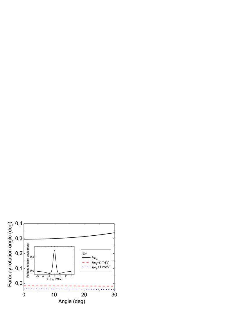
Figure 1: Faraday rotation angle by a single QW versus the angle of incidence for different energies close of the exciton resonance. $\hbar\omega_{0}=1.4$ eV, $\hbar\Gamma_{0}=0.026$ meV, $\hbar\gamma=0.5$ meV, Zeeman splitting is 0.1 meV. Inset shows Faraday rotation angle calculated as a function of energy for the same quantum well at normal light incidence.

The solution of linear equations (9) can be presented in the form

$$\Lambda_{x}=\alpha_{x}\Lambda_{0x}+\alpha_{y}\Lambda_{0y}\>,$$ (13)

$$\Lambda_{y}=\beta_{x}\Lambda_{0x}+\beta_{y}\Lambda_{0y}\>,$$

where

$$\alpha_{x}=\left({1+\frac{q_{z}}{2q}\frac{\Delta\omega_{p}-{\rm i}\Gamma_{0}}{\Omega^{+}}}\right)\frac{1}{\mathcal{D}}\>,\quad\alpha_{y}=\frac{{\rm i}q_{z}}{2q}\frac{\Delta\omega_{p}-{\rm i}\Gamma_{0}}{\mathcal{D}\Omega^{-}}\>,$$ (14)

$$\beta_{x}=-\frac{iq}{2q_{z}}\frac{\Delta\omega_{p}-{\rm i}\Gamma_{0}}{\mathcal{D}\Omega^{-}}\>,\quad\beta_{y}=\left({1+\frac{q}{2q_{z}}\frac{\Delta\omega_{p}-{\rm i}\Gamma_{0}}{\Omega^{+}}}\right)\frac{1}{\mathcal{D}}\>,$$

$$\mathcal{D}=\left({1+\frac{q}{2q_{z}}\frac{\Delta\omega_{p}-{\rm i}\Gamma_{0}}{\Omega^{+}}}\right)\left({1+\frac{q_{z}}{2q}\frac{\Delta\omega_{p}-{\rm i}\Gamma_{0}}{\Omega^{-}}}\right)-\left({\frac{\Delta\omega_{p}-{\rm i}\Gamma_{0}}{2\Omega^{-}}}\right)^{2}\>,$$

and $(\Omega^{\pm})^{-1}=(\omega_{+}-\omega-{\rm i}\gamma)^{-1}\pm(\omega_{-}-\omega-{\rm i}\gamma)^{-1}$. In order to find the reflection and transmission coefficients of the QW we should find the asymptotic values of the electric field far beyond the QW. Coming back to Eq. (7) and putting $z\to\pm\infty$ one easily obtains

$$E_{x}(z\to\pm\infty)=E_{0x}{\rm e}^{{\rm i}q_{z}z}+{\rm i}{\rm e}^{\pm{\rm i}q_{z}z}\frac{\pi Qq_{z}}{q^{2}}\left({\frac{\omega}{c}}\right)^{2}\left(\Sigma_{+}+\Sigma_{-}\right){\int\limits_{-\infty}^{+\infty}{\Phi(z^{\prime})}e^{\mp{\rm i}q_{z}z^{\prime}}dz^{\prime}}\>,$$ (15)

$$E_{y}(z\to\pm\infty)=E_{0y}{\rm e}^{{\rm i}q_{z}z}-\hskip 7.11317pt{\rm e}^{\pm{\rm i}q_{z}z}\frac{\pi Q}{q_{z}}\left({\frac{\omega}{c}}\right)^{2}\left(\Sigma_{-}-\Sigma_{+}\right){\int\limits_{-\infty}^{+\infty}{\Phi(z^{\prime})}e^{\mp{\rm i}q_{z}z^{\prime}}dz^{\prime}}\>.$$

The transmission and reflection coefficients are polarization-dependent and can be represented in the form of $2\times 2$ matrices $\hat{r}$ and $\hat{t}$ defined by

$${\bm{E}}(z\to-\infty)-{\bm{E}}_{0}e^{{\rm i}q_{z}z}=\hat{r}{\bm{E}}_{0}e^{{\rm i}q_{z}z}\>,\>{\bm{E}}(z\to+\infty)=\hat{t}{\bm{E}}_{0}e^{{\rm i}q_{z}z}\>.$$ (16)

Using Eqs. (13)–(16) one obtains after simple algebra the reflection matrix elements,

$$r_{xx}=\frac{{\rm i}\Gamma_{0}}{2}\left({\frac{1}{\Omega^{+}}+\frac{q}{q_{z}}\frac{\Delta\omega_{p}-{\rm i}\Gamma_{0}}{\left({\omega_{+}-\omega-{\rm i}\Gamma}\right)\left({\omega_{-}-\omega-{\rm i}\Gamma}\right)}}\right)\>,$$ (17)

$$r_{yy}=\frac{{\rm i}\Gamma_{0}}{2}\left({\frac{1}{\Omega^{+}}+\frac{q_{z}}{q}\frac{\Delta\omega_{p}-{\rm i}\Gamma_{0}}{\left({\omega_{+}-\omega-{\rm i}\Gamma}\right)\left({\omega_{-}-\omega-{\rm i}\Gamma}\right)}}\right)\>,$$

$$r_{xy}=-r_{yx}=\frac{\Gamma_{0}}{2\Omega^{-}\mathcal{D}}\>.$$

The transmission and reflection coefficients are interrelated by

$$t_{ij}=\delta_{ij}+r_{ij}\>,$$ (18)

where $\delta_{ij}$ is the Kronecker delta. Note that, due to the Zeeman splitting of the exciton resonance into a circularly polarized doublet, the coupling of light with an exciton leads to the mixing of TE and TM polarizations both in reflection and transmission. This results in the resonant Faraday and Kerr rotation and dichroism Brunetti:2006 .

Figure 1 shows the angle of rotation of the polarization plane of transmitted light with respect to the polarization plane of incident light (which is assumed to be TE-polarized) versus the angle of incidence for different energies close of the exciton resonance for the magnetic field of 2 T (the induced Zeeman splitting is 0.1 meV). We have considered a 10 nm GaAs QW with $\Gamma_{0}=0.026$ meV. The homogeneous broadening is 0.5 meV. The effect includes both linear-circular dichroism and Faraday rotation. The angle of Kerr rotation can be calculated by using the following equation, see, e.g., LandauLif ,

$$\theta_{K}=\frac{1}{2}\arctan{\frac{2{\rm Re}\{r_{yy}^{*}\tilde{r}_{xy}\}}{|r_{yy}|^{2}-|\tilde{r}_{xy}|^{2}}}\>.$$ (19)

Here $\tilde{r}_{xy}=r_{xy}/\cos{\theta}$. The Faraday rotation angle $\theta_{F}$ is obtained by the replacement $r_{ij}\to t_{ij}$. For small rotations a simplified equation $\theta_{K}\approx{\rm Re}\{r_{xy}/(r_{yy}\cos{\theta})\}$ can be applied. One can check that the effect is strongest at the resonance and decreases with the increasing angle of incidence.

III Dispersion of exciton-polaritons in microcavities subjected to the magnetic field

Let us now consider a QW embedded in the center of a planar microcavity in the external magnetic field parallel to the structure growth axis, Fig. 2. We shall calculate the dispersion of the exciton-polaritons in such a system using the generalized transfer matrix formalism. Then we compare this exact approach with a simple model of coupled oscillators where exciton and photon states are represented by the effective classical oscillators.

Figure 2: Schematic diagram of the microcavity with QW. Arrows show the direction of electromagnetic field propagation inside the cavity.

The eigenstates of the cavity can be found from the condition that a non-zero field exists inside the cavity without any external field. We choose the QW center as an origin $z=0$ and present the electric field inside the cavity (but outside the QW) in the form

$${\rm e}^{{\rm i}kx}\left({\bm{E}}^{+}_{L}{\rm e}^{{\rm i}q_{z}z}+{\bm{E}}^{-}_{L}{\rm e}^{-{\rm i}q_{z}z}\right)\hskip 8.53581pt\mbox{and}\hskip 8.53581pt{\rm e}^{{\rm i}kx}\left({\bm{E}}^{+}_{R}{\rm e}^{{\rm i}q_{z}z}+{\bm{E}}^{-}_{R}{\rm e}^{-{\rm i}q_{z}z}\right)\>,$$ (20)

respectively, on the left and right-hand side from the QW. The fields ${\bm{E}}^{\pm}_{L,R}$ are interrelated by the transfer matrix through the QW as follows

$$\hat{T}_{QW}\left(\begin{array}[]{c}{\bm{E}}_{L}^{+}\\ {\bm{E}}_{L}^{-}\end{array}\right)=\left(\begin{array}[]{c}{\bm{E}}^{+}_{R}\\ {\bm{E}}_{R}^{-}\end{array}\right)\>.$$ (21)

Here $\hat{T}_{QW}$ is a $4\times 4$ matrix, its explicit form is given later, and ${\bm{E}}^{\pm}_{L,R}$ are two-component columns with components $E_{L,x}^{+},E_{L,y}^{+}$ etc. According to Fig. 3 ${\bm{E}}_{L}^{+}$ and ${\bm{E}}_{R}^{-}$ can be expressed via ${\bm{E}}_{L}^{-}$ and ${\bm{E}}_{R}^{+}$ by

$${\bm{E}}_{L}^{+}=\hat{r}_{B}{\bm{E}}_{L}^{-}{\rm e}^{{\rm i}q_{z}\ell}\>,\>{\bm{E}}_{R}^{-}=\hat{r}_{B}{\bm{E}}_{R}^{+}{\rm e}^{{\rm i}q_{z}\ell}\>,$$ (22)

where $\ell$ is the width of the active layer and $\hat{r}_{B}$ is a $2\times 2$ diagonal matrix of reflection from the Bragg mirror. Note that, at oblique incidence ($q_{x}=k\neq 0$), its components $r_{B,xx}$ and $r_{B,yy}$ are different. Equations (22) can be interpreted as follows. A QW exciton creates the outgoing electromagnetic waves $\bm{E}_{L}^{-}$ and $\bm{E}_{R}^{+}$ propagating to the left and to the right, respectively. The waves reaching the Bragg mirror acquire the phase $q_{z}\ell/2$, the field reflected from the mirror returns to the QW with the phase $q_{z}\ell$ and the additional factors $r_{B,ii}$. Whence, we obtain equation (22) for the incoming waves. From Eqs. (21), (22) we arrive at the matrix dispersion equation

$$\hat{T}_{QW}\left(\begin{array}[]{c}\hat{r}_{B}{\bm{E}}_{L}^{-}{\rm e}^{{\rm i}q_{z}\ell}\\ {\bm{E}}_{L}^{-}\end{array}\right)=\left(\begin{array}[]{c}{\bm{E}}_{R}^{+}\\ \hat{r}_{B}{\bm{E}}_{R}^{+}{\rm e}^{{\rm i}q_{z}\ell}\end{array}\right)\>.$$ (23)

The considered structure is symmetric, therefore the solutions of Eq. (23) can be classified as even [${\bm{E}}_{L}^{\pm}={\bm{E}}^{\pm}_{R}$ in Eq. (23)] and odd (${\bm{E}}_{L}^{\pm}=-{\bm{E}}^{\pm}_{R}$) with respect to the mirror reflection in the QW plane. The electric field in odd solutions is uncoupled with the even lowest-exciton state, thus these modes are purely photonic. On the contrary, the even-parity cavity mode is coupled with the QW exciton to form mixed exciton-polariton modes. The matrix equation (23) is equivalent to four scalar equations. Among them, for the waves of certain parity, only two are linearly independent. If we present the transfer matrix in the block form

$$\hat{T}_{QW}=\left(\begin{array}[]{cc}\hat{T}^{(11)}&\hat{T}^{(12)}\\ \hat{T}^{(21)}&\hat{T}^{(22)}\end{array}\right)\>,$$ (24)

where $\hat{T}^{(ij)}$ are $2\times 2$ matrices, then, for the even modes, the dispersion equation relating the frequency $\omega$ with the in-plane wave vector $k$ can be reduced to

$${\rm det}(\hat{T}^{(21)}\hat{r}_{B}{\rm e}^{{\rm i}q_{z}\ell}+\hat{T}^{(22)}-\hat{r}_{B})=0\>.$$ (25)

Using the definition of reflection and transmission coefficients, Eq. (16), one can present the blocks $\hat{T}^{(ij)}$ in the form

$$T^{(11)}_{11} = (t_{xy}t_{xx}t_{yx}-t_{xy}r_{xx}r_{yx}-t_{xx}^{2}t_{yy}-t_{yx}r_{xx}r_{xy}+r_{yx}t_{xx}r_{xy}+r_{xx}^{2}t_{yy})/\Delta\>,$$ (26)

$$T^{(11)}_{12} = (t_{yx}t_{xy}^{2}-t_{xy}r_{yy}r_{xx}-t_{xy}t_{xx}t_{yy}-t_{yx}r_{xy}^{2}+r_{yy}t_{xx}r_{xy}+r_{xy}t_{yy}r_{xx})/\Delta\>,$$

$$T^{(11)}_{21} = (-t_{xx}t_{yy}t_{yx}+t_{xx}r_{yx}r_{yy}+t_{xy}t_{yx}^{2}+t_{yy}r_{xx}r_{yx}-r_{yx}^{2}t_{xy}-r_{xx}t_{yx}r_{yy})/\Delta\>,$$

$$T^{(11)}_{22} = (-t_{xx}t_{yy}^{2}+t_{xx}r_{yy}^{2}+t_{xy}t_{yx}t_{yy}+t_{yy}r_{xy}r_{yx}-r_{yy}t_{xy}r_{yx}-r_{xy}t_{yx}r_{yy})/\Delta\>,$$

$$\hat{T}^{(12)}=\frac{1}{\Delta}\left(\begin{array}[]{cc}{r_{xy}t_{yx}-r_{xx}t_{yy}}&{t_{xy}r_{xx}-t_{xx}r_{xy}}\\ {t_{yx}r_{yy}-t_{xx}r_{yx}}&{r_{yx}t_{xy}-r_{yy}t_{xx}}\end{array}\right)\>,$$ (29)

$$\hat{T}^{(21)}=\frac{1}{\Delta}\left(\begin{array}[]{cc}{r_{xx}t_{yy}-t_{xy}r_{yx}}&{r_{xy}t_{yy}-t_{xy}r_{yy}}\\ {r_{yx}t_{xx}-t_{yx}r_{xx}}&{t_{xx}r_{yy}-r_{xy}t_{yx}}\end{array}\right)$$ (32)

and

$$\hat{T}^{(22)}=\frac{1}{\Delta}\left(\begin{array}[]{cc}-t_{yy}&t_{xy}\\ t_{yx}&-t_{xx}\end{array}\right)\>,$$ (33)

where $\Delta=t_{xy}t_{yx}-t_{xx}t_{yy}$.

In general, Eq. (25) has four solutions for each incidence angle which corresponds to four exciton-polariton dispersion branches. The polarization of polariton eigenmodes is determined by the electric-field complex amplitudes $E_{x}$ and $E_{y}$. The degree of polariton circular polarization is given by the standard expression LandauLif

$$\rho_{c}=\frac{2{\rm Im}\{E^{\ast}_{x}E_{y}\}}{|E_{x}|^{2}+|E_{y}|^{2}}\>.$$ (34)

In the absence of an external magnetic field the cross-polarized reflection and transmission coefficients vanish, $r_{xy}=r_{yx}=t_{xy}=t_{yx}=0$, and Eq. (25) reduces to a couple of independent equations for TE- and TM-polarized polariton modes satisfying the dispersion equation ivchbook :

$$(2r_{ii}+1)r_{B,ii}{\rm e}^{{\rm i}q_{z}\ell}=1\>,$$ (35)

where $i=x$ (TM) or $i=y$ (TE). In this case exciton-polariton modes have definite linear polarizations.

In order to demonstrate underlying physics of the light-matter coupling we also put forward a simplified model of four coupled oscillators representing the TE- and TM- polarized optical modes of empty cavity and two excitonic modes split by the Zeeman interaction. The effective dispersion equation can be written as

$$\det\left({{\begin{array}[]{*{20}c}{\hbar\omega_{0}(k)-E\hfill}&{{\rm i}g\mu_{B}B/2\hfill}&{V/2\hfill}&0\hfill\\ {-{\rm i}g\mu_{B}B/2\hfill}&{\hbar\omega_{0}(k)-E\hfill}&0\hfill&{V/2\hfill}\\ {V/2\hfill}&0\hfill&{E_{ph}^{\left({\rm TE}\right)}(k)-E\hfill}&0\hfill\\ 0\hfill&{V/2\hfill}&0\hfill&{E_{ph}^{\left({\rm TM}\right)}(k)-E\hfill}\\ \end{array}}}\right)=0\>.$$ (36)

Here $V$ is the Rabi splitting determined by the system parameters, $E_{ph}^{\left({\rm TE}\right)}(k)$, $E_{ph}^{\left({\rm TM}\right)}(k)$ are dispersions of the TE and TM bare-cavity photons. We neglected the longitudinal-transverse splitting of the exciton.

The difference between this approach and the rigorous formalism presented above consists in (i) neglecting of the coupling of four polariton modes with all other light modes in the cavity and (ii) disregarding of the polarization dependence of the light-matter coupling constant $V_{R}$ goupalov .

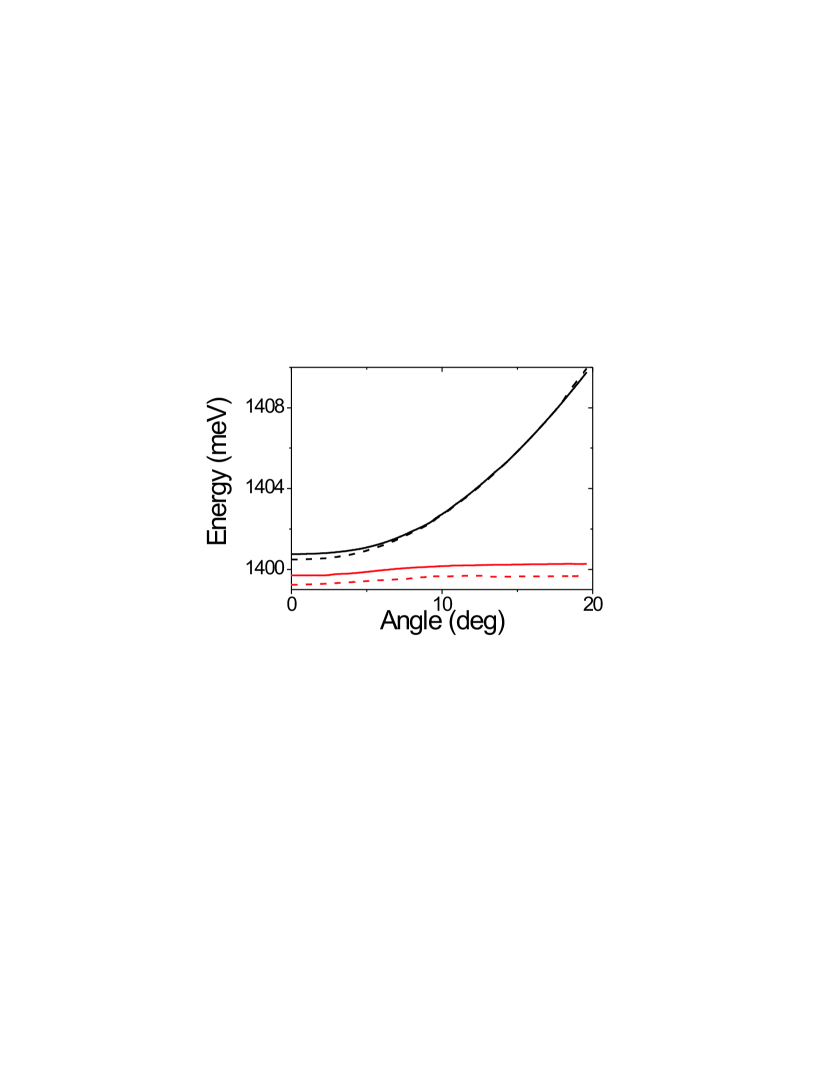
Figure 3: Dispersion of exciton-polaritons in the cavity in strong magnetic field $B=11.5$ T ($g\mu_{B}B=0.6$ meV) calculated for the exact Eq. (25). Red and black mark lower and upper polariton branches, correspondingly, and solid and dashed lines correspond to different polarizations. Cavity width is $\lambda=246$ nm. Other parameters the same as in Fig. 1.

Figure 3 shows the exact dispersion of cavity polaritons for an artificially high value of the magnetic field 11.5 T allowing to make visible all peculiarities of the dispersion. This field corresponds to the Zeeman splitting of 0.6 meV. We consider a $\lambda$-cavity with 10 nm GaAs QW (parameters are the same as in Fig. 1). The distributed Bragg reflectors (DBRs) are typical 20-period GaAs/Al_0.18Ga_0.82As mirrors. Approximate dispersion curves calculated from Eq. (36) are not shown, because they do not differ from the exact one in the range of angles considered. Four branches of exciton-polaritons having a characteristic non-parabolic dispersion are clearly seen. The anticrossings take place between branches having the same circular polarization. In such a strong field, the polariton eigenstates are almost completely circularly polarized, so we do not show their polarization degree in this case.

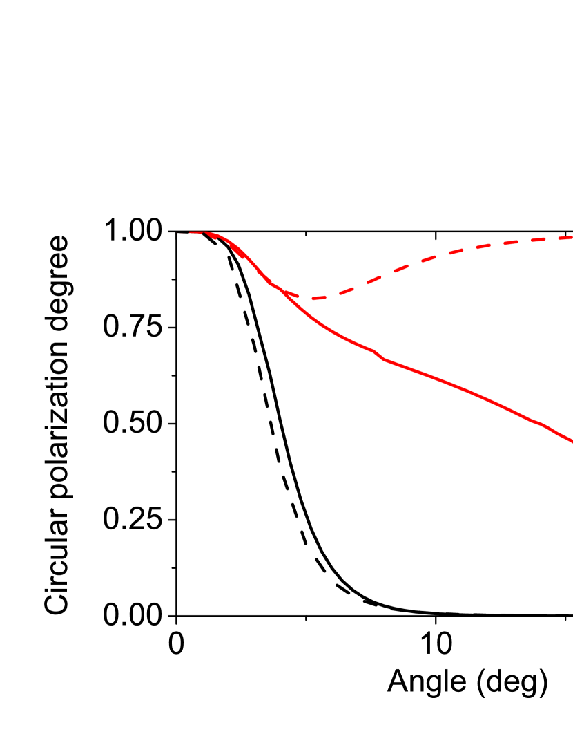
Figure 4: Circular polarization degree in the case of magnetic field $B=0.04$ T ($g\mu_{B}B=2\times 10^{-3}$ meV) (solid line – exact model, dashed line – approximate model; red color shows exciton-like branch and black color shows photon-like branch). Only branches with positive polarization degree are shown.

However, we do show the the circular polarization degree of the cavity eigenstates in the exact and approximate models for a small magnetic field of 0.04 T (Zeeman splitting is 2 $\mu$eV) in figure 4. The results match well except for the exciton-like branch (red), the difference coming from the fact that in the exact model the exciton eigenstates are circularly polarized, whereas in the approximate model they are linearly polarized (their TE-TM splitting is taken into account). The circular polarization degree has been calculated using Eq. (34) in both models, the difference being that in one case the complex amplitudes are the eigenvectors of exact system Eq. (25) and in the other case they are the eigenvectors of approximate system Eq. (36). For such a small field, the splittings that appear in the polaritonic branches, are invisible relative to the Rabi splitting, therefore we do not show the corresponding dispersions.

IV Kerr and Faraday rotation in quantum microcavities

In this section we consider Kerr and Faraday effects in quantum microcavities. It is assumed that $s$ or $p$ polarized light is incident on a microcavity from the vacuum and the rotation of polarization plane of reflected (Kerr effect) and transmitted (Faraday effect) wave is monitored as a function of incidence angle.

The Kerr and Faraday rotation angles can be determined once the matrices of amplitude reflection (transmission) coefficients $r_{c,ij}$ ($t_{c,ij}$) of the whole microcavity are known. The latter can be found from the microcavity transfer matrix $\hat{T}_{\rm qmc}$ which, in accordance with its definition, can be recast as a product

$$\hat{T}_{\rm qmc}=\hat{T}_{B}\hat{T}_{l}\hat{T}_{QW}\hat{T}_{l}\hat{T}_{B},$$ (37)

where $\hat{T}_{B}$ is the transfer matrix through the Bragg mirror, $\hat{T}_{l}$ is the transfer matrix through a half of the cavity and $T_{QW}$ is the quantum well transfer matrix, determined in Eqs. (24), (26)–(33). The transfer matrix through the homogeneous layer of the thickness $l$ is diagonal and given by

$$\hat{T}_{l}=\left(\begin{array}[]{cc}e^{\mathrm{i}q_{z}\ell/2}\hat{I}&0\\ 0&e^{-\mathrm{i}q_{z}\ell/2}\hat{I}\end{array}\right),$$ (38)

where $\hat{I}$ is the $2\times 2$ unit matrix.

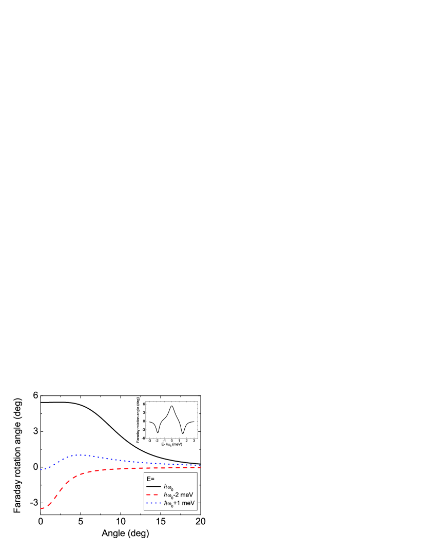
Figure 5: Faraday rotation angle as a function of the incidence angle for the $s$ polarized light. The QW and cavity parameters are the same as before. The Zeeman splitting is 0.1 meV. Inset shows energy dependence of Faraday rotation angle at the same parameters at normal light incidence.

For example, the transmission and reflection coefficients in the $s$ polarization can be determined from the following system of equations

$$\hat{T}_{qmc}\left(\begin{array}[]{c}0\\ 1\\ r_{c,xy}\\ r_{c,yy}\end{array}\right)=\left(\begin{array}[]{c}t_{c,xy}\\ t_{c,yy}\\ 0\\ 0\end{array}\right).$$ (39)

Figure 5 shows calculated Faraday rotation angle at oblique incidence as a function of incidence angle. An inset in the figure presents the Faraday rotation angle as a function of the energy. The function shows a non-monotonous behaviour reflecting the resonant character of light reflection and transmission in microcavities. The figure clearly demonstrates that Faraday rotation angles are almost by an order of magnitude larger than those for the Faraday rotation in the case of a single quantum well. This enhancement can be interpreted as a result of multiple passage of a photon inside a cavity Kavokin:1997 .

Namely, consider a cavity mode as a beam of light travelling back and forth inside the cavity. Let $N$ be an average number of photon round trips between the Bragg mirrors made during its life-time ($N\sim Q$, where $Q$ is the cavity quality factor). At each trip the polarization plane of the photon exhibits a rotation by $\delta\theta$ and the Faraday effect is strongly enhanced. The observable Faraday rotation angle is smaller than $N\delta\theta$ because there is a finite probability for the photon to escape cavity after any number of passages Kavokin:1997 . The absolute value of the Faraday rotation angle decreases with the increase of the incidence angle, due to the decrease of the polariton lifetime in the cavity. In average, the polaritons make less rount-trips inside the cavity at oblique angles than at normal angle. We note that the Kerr rotation angles (observed in reflection geometry) are smaller than the Faraday rotation angles because the light reflection from the microcavity is dominated by a surface reflection of the Bragg mirror.

V Conclusions

In conclusion, we have analyzed the dispersion of the exciton-polaritons in a microcavity subjected into the external magnetic field taking in account both Zeeman splitting of the exciton and TE-TM splitting of the photonic modes. We have shown that the polarization of the polariton eigenstates is neither linear nor circular, but elliptical, in general. It is very sensitive to the polariton in-plane wave vector as well as to the detuning between the exciton and photon modes.

We have also studied theoretically the Faraday rotation in the planar microcavities. We found that the giant Faraday rotation due to the multiple passages of light across the quantum well takes place at normal incidence, while this effect is reduced at oblique incidence angles.

- (1) See, e.g., papers in the special issue on microcavities, Semicond. Sci. Technol. 18 , N 10 (2003) or A.V. Kavokin and G. Malpuech, Cavity Polaritons, Elsevier, Amsterdam, 2003.
- (2) M. Richard, J. Kasprzak, R. André, R. Romestain, Le Si Dang, G. Malpuech, and A. Kavokin, Phys. Rev. B 72, 201301 (2005).
- (3) P.G. Savvidis, J.J. Baumberg, R. M. Stevenson, M.S. Skolnick, D.M. Whittaker, and J.S. Roberts, Phys. Rev. Lett. 84, 1547, (2000).
- (4) A. Imamoglu and J.R. Ram, Phys. Lett. A 214, 193 (1996).
- (5) J. Kasprzak, M. Richard, S. Kundermann, A. Baas, P. Jeambrun, J.M.J. Keeling, F.M. Marchetti, M.H. Szymańska, R. André, J.L. Staehli, V. Savona, P.B. Littlewood, B. Deveaud, and Le Si Dang, Nature 443, 409 (2006).
- (6) S. Christopoulos et al, Phys. Rev. Lett. 98, 126405 (2007).
- (7) I.A. Shelykh, Yu.G. Rubo, G. Malpuech, D.D. Solnyshkov, and A.V. Kavokin, Phys. Rev. Lett. 97, 66402 (2006).
- (8) I. Carusotto and C. Ciuti, Phys. Rev. Lett. 93, 166401 (2004).
- (9) I.A. Shelykh, A.V. Kavokin, and G. Malpuech, phys. stat. sol. (b) 242, 2271 (2005).
- (10) Yu.G. Rubo, A.V. Kavokin, and I.A. Shelykh, Phys. Lett. A 358, 227 (2006).
- (11) M.Z. Maialle, D.E. de Andrada e Silva, and L.J. Sham, Phys. Rev. B 47, 15776 (1993).
- (12) G. Panzarini, L.C. Andreani, A. Armitage, D. Baxter, M.S. Skolnick, V.N. Astratov, J.S. Roberts, A.V. Kavokin, M.R. Vladimirova, and M.A. Kaliteevski, Phys. Rev. B 59, 5082 (1999).
- (13) J. Tignon, R. Ferreira, J. Wainstain, C. Delalande, P. Voisin, M. Voos, R. Houdré, U. Oesterle, and R.P. Stanley, Phys. Rev. B 56, 4068 (1997).
- (14) J.D. Berger, O. Lyngnes, H.M. Gibbs, G. Khitrova, T.R. Nelson, E.K. Lindmark, A.V. Kavokin, M.A. Kaliteevski, and V.V. Zapasskii, Phys. Rev. B 54, 1975 (1996).
- (15) A. Armitage, T.A. Fisher, M.S. Skolnick, D.M. Whittaker, P. Kinsler, and J.S. Roberts, Phys. Rev. B 55, 16395 (1997).
- (16) P. Renucci, T. Amand, and X. Marie, Physica E 17, 329 (2003).
- (17) A. Brunetti, M. Vladimirova, D. Scalbert, R. André, D. Solnyshkov, G. Malpuech, I.A. Shelykh, and A.V. Kavokin, Phys. Rev. B 73, 205337 (2006).
- (18) A. Brunetti, M. Vladimirova, D. Scalbert, M. Nawrocki, A.V. Kavokin, I.A. Shelykh, and J. Bloch, Phys. Rev. B 74, 241101 (2006).
- (19) L.D. Landau and E.M. Lifshits, The Classical Theory of Fields, Volume 2 (Course of Theoretical Physics Series) Elsevier, 1980.
- (20) V. Savona, L.C. Andreani, P. Schwendimann, and A. Quattropani, Solid State Commun. 93, 733 (1995).
- (21) A.V. Kavokin and M.A. Kaliteevski, Solid State Commun. 95, 859 (1995).
- (22) L.C. Andreani, F. Tassone, and F. Bassani, Solid State Commun. 77, 641 (1991).
- (23) E.L. Ivchenko, Sov. Phys. Solid State 33, 1344 (1992).
- (24) F. Tassone, F. Bassani, and L.C. Andreani, Phys. Rev. B 45, 6023 (1992).
- (25) A.V. Kavokin, M.R. Vladimirova, M. A. Kaliteevski, O. Lyngnes, J.D. Berger, H.M. Gibbs, and G. Khitrova, Phys. Rev. B 56, 1087 (1997).
- (26) A.V. Kavokin, A.I. Nesvizhskii, and R.P. Seisyan, Sov. Phys. Semicond. 27, 530 (1993).
- (27) E.L. Ivchenko, Optical spectroscopy of semiconductor nanostructures (Alpha Science, Harrow UK, 2005).
- (28) S.V Goupalov, E.L. Ivchenko, and A.V. Kavokin, JETP 86, 388 (1998).