Stabilization under shared communication
with message losses and its limitations

Abstract

We consider a synthesis problem for a remotely controlled linear system where the communication is constrained because of the shared and unreliable nature of the channel. Modeling the constraints by a periodic transmission scheme and random message losses, we present an $H^{\infty}$ design framework and study the limitations in the communication required for stabilization.

1 Introduction

We consider a remote control system in which the plant has multiple sensors and actuators connected to a controller over network channels. In particular, we follow the approach of [12] and model two constraints due to the shared and unreliable nature of the channels. One is a periodic transmission scheme under which the sensor/actuator nodes take turns to transmit messages in a periodic manner. The other constraint is that each transmission is subject to random loss or delay due to congestion or error in the communication. Here, it is assumed that if a message is delayed, then it is considered lost. The losses are modeled as Bernoulli processes where the loss probabilities are a priori known. Further, the controller uses the information regarding the losses of the messages that it receives as well as those that it sends; the latter is realized by the use of acknowledgement messages with a one-step delay.

Under this setup, in [12], a synthesis method for stochastic stabilization of linear time-invariant plants and for optimization under an $H^{\infty}$-type norm criterion has been proposed. It is based on a necessary and sufficient condition expressed in the form of linear matrix inequalities. Hence, we can employ efficient algorithms to investigate the effects of the communication constraints on control performance. Another advantage of this approach is that because of the norm criterion used in the paper, the design can be viewed as a natural extension of deterministic robust control methods. We also note that the synthesis method has been found useful in developing subband coding techniques for networked control [15].

The focus in this paper is on the limitations in stabilization due to the message losses and in particular on upper bounds for the loss probabilities above which stabilization cannot be accomplished. It turns out that such bounds can analytically be obtained. We emphasize that the bounds are expressed in terms of the unstable poles of the plant together with parameters in the communication scheme.

There are two characteristics of the approach in this paper. One is that, by following [20], we view the remote control system as a special case of Markovian jump systems (see, e.g., [16, 2]). This is a natural approach especially when acknowledgements are available on the controller side. The other is that we employ the periodic transmission scheme which has been considered in [18, 14, 9]. In this paper, we show critical bounds on losses which are generalizations of the results for the simpler case of SISO plant with single-rate communication.

Similar bounds on critical loss probabilities have appeared in the recent literature. In the context of remote control, early studies on such probabilities include [8, 21]. In [3], a synthesis problem for stochastic stabilization has been considered, and a necessary and sufficient bound for the state feedback case is found. The result is extended in [4] to various remote control configurations. One difference from the approach in this paper is that the controllers are limited to deterministic time-invariant systems. In [10], it is shown in an LQ type problem that the availability of acknowledgement messages has a crucial impact on controller designs and also on the loss probabilities. This issue is further studied in [7, 22], where LQG problems over lossy channels are investigated. Also, an estimation scheme with filters on the sensor side has been proposed in [23]. For the case of nonlinear systems, the treatment of random losses in the channel is studied in [19].

This paper is organized as follows: In Section 2, we introduce a class of stochastic systems and some definitions. In Section 3, we review the remote control problem considered in [12]. Then, the stabilization problem of this paper and the main results are presented in Section 4. To illustrate the results, we provide a numerical example in Section 5. Finally, concluding remarks are given in Section 6. We note that this paper is an extended version of [11].

2 Periodic systems with random switchings

In this section, we introduce a class of systems called periodic systems with random switchings and provide some definitions and a preliminary result [12].

Consider the following periodic system $G_{0}$ with random switchings:

$$\begin{split}x_{k+1}&=A_{k,\theta(k)}x_{k}+B_{k,\theta(k)}w_{k},\\ z_{k}&=C_{k,\theta(k)}x_{k}+D_{k,\theta(k)}w_{k},\end{split}$$ (1)

where $x_{k}\in{\mathbb{R}}^{n}$ is the state, $w_{k}\in{\mathbb{R}}^{m}$ is the input, $z_{k}\in{\mathbb{R}}^{p}$ is the output, and $\theta_{k}\in\mathcal{I}_{M}$ is the mode of the system with the index set $\mathcal{I}_{M}:=\{0,1,\ldots,M-1\}$. The mode $\theta_{k}$ is assumed to be an independent and identically distributed (i.i.d.) stochastic process determined by the probabilities $\alpha_{i}=\mathrm{Prob}\{\theta_{k}=i\}$, $i\in\mathcal{I}_{M}$. The system matrices are $N$-periodic, that is, e.g., $A_{k+N,i}=A_{k,i}$ for each $i\in\mathcal{I}_{M}$ and $k\in{\mathbb{Z}}_{+}$.

Let $\mathcal{F}_{k}$ be the sigma-field generated by $\theta_{[0,k]}$. We assume that the input $w_{k}$ is $\mathcal{F}_{k-1}$-measurable for each $k$. Moreover, $w$ is assumed to be in $l^{2}$ in the sense that $E[\sum_{k=0}^{\infty}\lvert w_{k}\rvert^{2}]<\infty$, where the expectation $E[\,\cdot\,]$ is taken over the statistics of $\theta$. Let the norm of such signals be $\lVert w\rVert:=E[\sum_{k=0}^{\infty}\lvert w_{k}\rvert^{2}]^{1/2}$. We denote by $\mathcal{W}$ the space of such signals.

For the system $G_{0}$ in (1), we employ the following notion of stability. The system (1) with $w_{k}\equiv 0$ is said to be stochastically stable if for any initial condition $x_{0}$,

$$E\bigl{[}\sum_{k=0}^{\infty}\lvert x_{k}\rvert^{2}\bigl{|}\ x_{0}\bigr{]}<\infty.$$

We next introduce the $l^{2}$-induced norm of the system $G_{0}$. Suppose that $G_{0}$ is stochastically stable and the initial state is $x_{0}=0$. Then, we define the $l^{2}$-induced norm of the system as follows:

$$\lVert G_{0}\rVert:=\sup_{w\in\mathcal{W},w\neq 0}\frac{\lVert z\rVert}{\lVert w\rVert}.$$

In [12], characterizations of the stability and the norm of the system $G_{0}$ have been obtained. They are stated in terms of linear matrix inequalities (LMIs). We present the stability result in the following.

Lemma 2.1

The system $G_{0}$ in (1) is stochastically stable if and only if there exists an $N$-periodic matrix $P_{k}\in{\mathbb{R}}^{n\times n}$ such that $P_{k}=P_{k}^{T}>0$ and

$$\sum_{i\in\mathcal{I}_{M}}\alpha_{i}A_{k,i}^{T}P_{k+1}A_{k,i}-P_{k}<0~{}~{}\text{for $k\in\mathcal{I}_{N}$},$$ (2)

where $\mathcal{I}_{N}:=\{0,\ldots,N-1\}$.

3 Remote control system and its stabilization

In this section, we first present the remote control system setup that has been studied in [12]. There, an optimal controller design method under an $H^{\infty}$ norm criterion is proposed. In this paper, we consider the analytic bounds on the loss probabilities to achieve stabilization of this system.

Consider the remote control system depicted in Fig. 1. The generalized plant $G$ is a discrete-time system and has a state-space equation of the following form:

$$\begin{split}x_{k+1}&=Ax_{k}+B_{1}w_{k}+B_{2}u_{k},\\ z_{k}&=C_{1}x_{k}+D_{11}w_{k}+D_{12}u_{k},\\ y_{k}&=C_{2}x_{k}+D_{21}w_{k},\end{split}$$ (3)

where $x_{k}\in{\mathbb{R}}^{n}$ is the state, $w_{k}\in{\mathbb{R}}^{m_{1}}$ is the exogenous input, $u_{k}\in{\mathbb{R}}^{m_{2}}$ is the control input, $z_{k}\in{\mathbb{R}}^{p_{1}}$ is the controlled output, and $y_{k}\in{\mathbb{R}}^{p_{2}}$ is the measurement output. We assume that $(A,B_{2})$ is controllable and $(A,C_{2})$ is observable.

Using a shared communication channel, a remote controller is connected to multiple sensors and actuators. Due to the bandwidth limitation in the channel, we assume that at each discrete-time instant, only one of the sensors or actuators can transmit a message over the channel. For efficient communication under this constraint, the transmission of the messages is periodic and is a priori fixed. We now describe this scheme.

Let the period be $N\geq p_{2}+m_{2}$. We index the sensors from 1 to $p_{2}$ and fix the order of transmissions within the period $N$ as follows: Let the index set be $\mathcal{I}_{p_{2}+1}:=\{0,1,\ldots,p_{2}\}$. Then, introduce the vector $s_{1}\in\mathcal{I}_{p_{2}+1}^{N}$ called the switching pattern for the sensor side. This specifies that at time $k=lN+r$ with $r=0,1,\ldots,N-1$, the sensor indexed as $s_{1}(r+1)$ is allowed to send a message; if $s_{1}(r+1)$ is zero, no communication takes place. For example, let $N=5$, $p_{2}=2$, and $s_{1}=[1,1,2,0,0]$. In this case, sensor 1 transmits at $k=0,1,5,6,\ldots$ while sensor 2 transmits at $k=2,7,\ldots$, and there is no communication at $k=3,4,8,9,\ldots$. Similarly, we introduce the switching pattern $s_{2}\in\mathcal{I}_{m_{2}+1}^{N}$ for the $m_{2}$ actuators; this one determines the periodic transmission from the controller to the actuators.

Figure 1: Remote control over a shared channel

We give some notation for the periodic switchings. First, let $e_{p,i}\in{\mathbb{R}}^{p}$, $i=1,\ldots,p$, be the unit vectors given by $e_{p,i}:=[0\cdots 0\;1\;0\cdots 0]$, where the $i$th element equals $1$ and the rest are zero. Now, the switch boxes $S_{1}$ and $S_{2}$ in Fig. 1 are $N$-periodic matrices defined for $k=lN+r$, $r=0,1,\ldots,N-1$, as

$$S_{1,k} :=e_{p_{2},i}^{T},~{}~{}\text{if $s_{1}(r+1)=i$},$$

$$S_{2,k} :=e_{m_{2},j},~{}~{}\text{if $s_{2}(r+1)=j$}.$$

The channel is further constrained by being unreliable due to congestion or delay, and hence transmitted messages randomly are lost. Denote by $\theta_{1,k},\theta_{2,k}\in\{0,1\}$ the stochastic processes for the message losses, respectively, from the sensors to the controller and from the controller to the actuators. If $\theta_{i,k}=0$, then the message at time $k$ is lost, and otherwise, it arrives. They are assumed to be i.i.d. Bernoulli processes determined by

$$\alpha_{1}:=\mathrm{Prob}\{\theta_{1,k}=0\}~{}~{}\text{and}~{}~{}\alpha_{2}:=\mathrm{Prob}\{\theta_{2,k}=0\}$$

for $k\in{\mathbb{Z}}_{+}$. Letting $\mathcal{F}_{i,k}$ be the sigma-field generated by $\theta_{i,[0,k]}$, $i=1,2$, we assume that the disturbance $w_{k}$ is $\mathcal{F}_{1,k-1}$- and $\mathcal{F}_{2,k-1}$-measurable. Further, the disturbance is assumed to be in the space $\mathcal{W}$ as defined in Section 2.

The overall plant $\tilde{G}$ including the switches $S_{1}$ and $S_{2}$ and the message loss processes $\theta_{1}$ and $\theta_{2}$ is periodically time varying with period $N$ and with random switchings. The state-space equation of $\tilde{G}$ can be expressed as

$$\begin{split}x_{k+1}&=Ax_{k}+B_{1}w_{k}+\theta_{2,k}B_{2}S_{2,k}\hat{u}_{k},\\ z_{k}&=C_{1}x_{k}+D_{11}w_{k}+\theta_{2,k}D_{12}S_{2,k}\hat{u}_{k},\\ \hat{y}_{k}&=\theta_{1,k}S_{1,k}(C_{2}x_{k}+D_{21}w_{k}).\end{split}$$ (4)

In Fig. 1, $K$ is the controller to be designed. We allow it to also be $N$-periodic. Further, we assume that the control $u_{k}$ is $\mathcal{F}_{1,k}$- and $\mathcal{F}_{2,k-1}$-measurable. That is, at time $k$, $\theta_{1,k}$ and $\theta_{2,k-1}$ are known to the controller. This is realized by the use of acknowledgements from the actuators regarding the arrival of the control input $u_{k}$ with a one-step delay.

The controller takes a state-space form as follows:

$$\begin{split}\xi_{k}&=\hat{A}_{k-1,\theta_{1}(k-1),\theta_{2}(k-1)}\xi_{k-1}+\hat{B}_{k-1,\theta_{2}(k-1)}\hat{y}_{k-1},\\ \hat{u}_{k}&=\hat{C}_{k,\theta_{1}(k)}\xi_{k}+\hat{D}_{k}\hat{y}_{k},\end{split}$$ (5)

where $\xi_{k}\in{\mathbb{R}}^{n}$ is the state whose dimension is the same as that of the plant. The system matrices are $N$-periodic in $k$: For example, $\hat{A}_{k+N,i,j}=\hat{A}_{k,i,j}$ for $k\in{\mathbb{Z}}_{+}$ and $i,j\in\{0,1\}$. Notice that the state equation is expressed for the recursion at time $k$. At this point, $\theta_{2,k-1}$ is available at the controller through an acknowledgement. Thus, while the $A$- and $B$-matrices make use of this information, the $C$- and $D$-matrices can not. On the other hand, the $B$- and $D$-matrices do not use $\theta_{1,k}$ because $\theta_{1,k}=0$ means no input, $\hat{y}_{k}=0$.

Let the overall closed-loop system in Fig. 1 be $F_{l}(\tilde{G},K)$. This system is $N$-periodic and has random switchings with 4 modes: $(\theta_{1,k},\theta_{2,k})=(0,0),(0,1),(1,0),(1,1)$. It thus falls in the class of systems considered in Section 2.

In [12], we have provided an optimal synthesis method under an $H^{\infty}$ criterion. More specifically, the method solves the following problem: For the system in Fig. 1, given a scalar $\gamma>0$ and switching patterns $s_{1}$ and $s_{2}$, design a controller $K$ of the form (5) such that the closed-loop system $F_{l}(\tilde{G},K)$ is stochastically stable and satisfies $\lVert F_{l}(\tilde{G},K)\rVert<\gamma$. A necessary and sufficient condition for this problem has been derived in the form of LMIs. Thus, using this method, we can numerically check whether loss probabilities $\alpha_{1}$ and $\alpha_{2}$ are small enough to accomplish stabilization.

4 Limitations in loss probabilities for stabilization

In this section, we present several upper bounds for the loss probabilities in the channel which must be met to achieve stabilization. Hence, the bounds represent the maximum allowable probabilities. We show that for some specific setups, the bounds become necessary and sufficient.

For the problem of stabilization, we assume no disturbance, i.e., $w_{k}\equiv 0$, throughout this section. Hence, we consider the system setup in Fig. 2. We denote by $G_{22}$ the $(2,2)$-block of the generalized plant $G$. To simplify the notation, replace the triple $(A,B_{2},C_{2})$ with $(A,B,C)$. Therefore, the realization of $G_{22}$ is given by

$$\begin{split}x_{k+1}&=Ax_{k}+Bu_{k},\\ y_{k}&=Cx_{k},\end{split}$$ (6)

where $x_{k}\in{\mathbb{R}}^{n}$, $u_{k}\in{\mathbb{R}}^{m_{2}}$, and $y_{k}\in{\mathbb{R}}^{p_{2}}$. We assume that $A$ is an unstable matrix, that is, it has at least one eigenvalue whose absolute value is larger than $1$. Denote by $\lambda_{i}$, $i=0,1,\ldots,n-1$, the eigenvalues of $A$.

Here, due to the channel on the sensor side, the measurement $\hat{y}$ that the controller receives is

$$\hat{y}_{k}=\theta_{1,k}S_{1,k}y_{k},$$

where the behavior of the switch box $S_{1}$ is determined by the switching pattern $s_{1}$. The control signal $\hat{u}$ transmitted by the controller and the received signal $u$ at the actuator side are related by

$$u_{k}=\theta_{2,k}S_{2,k}\hat{u}_{k}.$$ (7)

Similarly, the periodic switch box $S_{2}$ is specified by the switching pattern $s_{2}$.

In the following, we study three different configurations and derive upper bounds for the loss probabilities.

Figure 2: Stabilization with periodic transmission

4.1 State feedback under single rate transmission

The first is the state feedback case with a single-rate channel on the actuator side.

In the system in Fig. 2, assume $C=I$ in (6) and $\alpha_{1}=0$ (that is, $\theta_{1,k}\equiv 1$). The transmissions are assumed to be single rate in that $S_{i,k}\equiv I$ for $i=1,2$; we thus take $N=1$. Furthermore, we assume that the plant is single input ($m_{2}=1$). Hence, the control input in (7) becomes

$$u_{k}=\theta_{2,k}Fx_{k},$$ (8)

where $F\in{\mathbb{R}}^{1\times n}$ is the state feedback gain matrix. Recall that $\theta_{2,k}\in\{0,1\}$ is the loss process determined by $\alpha_{2}=\mathrm{Prob}\{\theta_{2,k}=0\}$ for $k\in{\mathbb{Z}}_{+}$.

The following proposition provides an upper bound for the loss probability $\alpha_{2}$. This result has been given in [3].

Proposition 4.1

For the system $G_{22}$ in (6), there exists a state feedback gain $F$ in (8) such that the closed-loop system is stochastically stable if and only if the loss probability $\alpha_{2}$ is sufficiently small that

$$\alpha_{2}<\frac{1}{\prod_{\lvert\lambda_{i}\rvert>1}\lvert\lambda_{i}\rvert^{2}}.$$ (9)

The proof of this proposition is given in the Appendix. The approach in this paper is based on jump systems results using Lemma 2.1. We have clarified the critical loss probabilities in terms of the inequality arising in stochastic stability of such systems (see Lemma A.1 (ii)).

The result indicates that the unstable poles of the plant have a direct influence on the allowable loss rates in the channel for stochastic stability. The bound above has been found in [3], where the relation between state feedback stabilization over an unreliable channel and an optimal quantizer design problem has been discussed.

4.2 Remote control with periodic transmission

In this subsection, we consider the remote control case with the periodic transmission scheme introduced in Section 3.

Consider the system in Fig. 2. Here, the controller $K$ is limited to the observer-based one as follows:

$$\xi_{k} =A\xi_{k-1}+Bu_{k-1}+L_{k-1,\theta_{2}(k-1)}\left(\theta_{1,k-1}S_{1,k-1}C\xi_{k-1}-\hat{y}_{k-1}\right),$$ (10)

$$\hat{u}_{k} =F_{k,\theta_{1}(k)}\xi_{k},$$

where $\xi_{k}\in{\mathbb{R}}^{n}$, and $F_{k,\theta_{1}(k)}$ and $L_{k,\theta_{2}(k-1)}$ are the feedback and observer gains, respectively. These gains are $N$-periodic as, e.g., $F_{k+N,i}=F_{k,i}$ for all $k$ and $i$.

We first consider the case when $G_{22}$ is SISO. Note that in this case, the switch boxes $S_{1}$ and $S_{2}$ take values of either $0$ or $1$ and hence function as discrete-time periodic samplers. Their periodic behaviors are specified by the switching patterns $s_{i}\in\{0,1\}^{N}$, $i=1,2$. We denote by $N_{i}$ the number of $1$ in the pattern $s_{i}$ for $i=1,2$. As a special class of switching patterns, we introduce those called periodic vectors which take the following form:

$$s_{i}=[\overbrace{1\,0\,\cdots~{}0}^{N/N_{i}}\,\cdots\,\overbrace{1\,0\,\cdots\,0}^{N/N_{i}}]\in{\mathbb{R}}^{N}.$$ (11)

Some simple examples are $s_{i}=[1\,0\,\cdots\,0]$ when $N_{i}=1$, and $s_{i}=[1\,\cdots\,1]$ when $N_{i}=N$.

We are now ready to state the result on the loss probabilities for this setup.

Proposition 4.2

Suppose the switching patterns $s_{1}$ and $s_{2}\in\{0,1\}^{N}$ are in the periodic vector form in (11), and have, respectively, $N_{1}$ and $N_{2}$ entries of $1$. Then, for the system $G_{22}$ in (6), there exists a controller $K$ of the form (10) such that the closed-loop system is stochastically stable if and only if the loss probabilities $\alpha_{1}$ and $\alpha_{2}$ satisfy

$$\alpha_{1} <\frac{1}{\prod_{\lvert\lambda_{i}\rvert>1}\lvert\lambda_{i}\rvert^{2N/N_{1}}},$$ (12)

$$\alpha_{2} <\frac{1}{\prod_{\lvert\lambda_{i}\rvert>1}\lvert\lambda_{i}\rvert^{2N/N_{2}}}.$$ (13)

Proof :  Let the estimation error be $e_{k}:=x_{k}-\xi_{k}$. The closed-loop dynamics can be expressed as

$$x_{k+1} =(A+\theta_{2,k}BS_{2,k}F_{k,\theta_{1}(k)})x_{k}-\theta_{2,k}BS_{2,k}F_{k,\theta_{1}(k)}e_{k},$$ (14)

$$e_{k+1} =(A+\theta_{1,k}L_{k,\theta_{2}(k)}S_{1,k}C)e_{k}.$$ (15)

The error system (15) is decoupled from the state $x_{k}$ and in particular from the loss process $\theta_{2,k}$. Using this fact and the structure in the switching pattern $s_{1}$, we can show by Lemma 2.1 that to guarantee stochastic stability of this system, it is necessary and sufficient that there exists an observer gain that is independent of $k$ and $\theta_{2,k}$. The resulting system $e_{k+1}=(A+\theta_{1,k}LS_{1,k}C)e_{k}$ is periodic with period $\tilde{N}_{1}:=N/N_{1}$.

We now look at its dual system $z_{k+1}=(A^{T}+\theta_{1,k}C^{T}S_{1,k}L^{T})z_{k}$ with $z_{k}\in{\mathbb{R}}^{n}$ and express it in the so-called lifted form as follows: Let $\tilde{z}_{k}=z_{k\tilde{N}_{1}}$. Then, the lifted system is

$$\tilde{z}_{k+1}=\left[(A^{T})^{\tilde{N}_{1}}+\theta_{1,k\tilde{N}_{1}}(A^{T})^{\tilde{N}_{1}-1}C^{T}L^{T}\right]\tilde{z}_{k}.$$

Thus, by Proposition 4.1, there exists a stabilizing gain $L^{T}$ if and only if

$$\mathrm{Prob}\{\theta_{1,k\tilde{N}_{1}}=0\}<\frac{1}{\prod_{\lvert\tilde{\lambda}_{i}\rvert>1}\lvert\tilde{\lambda}_{i}\rvert^{2}},$$

where $\tilde{\lambda}_{i}$, $i=0,1,\ldots,n-1$, are the eigenvalues of $A^{\tilde{N}_{1}}$. However, since the loss process $\theta_{1,k}$ is i.i.d., the inequality above is equivalent to (13).

Similarly, we can show that the autonomous system $x_{k+1}=(A+\theta_{2,k}BS_{2,k}F_{k,\theta_{1}(k)})x_{k}$ of (14) can be stabilized if and only if (12) holds. This implies that a necessary and sufficient condition to stabilize the closed-loop system via output feedback is that the inequalities (12) and (13) hold. $\square$

This proposition is a generalization of Proposition 4.1 in two directions. First, it extends the result for the periodic transmission scheme. In particular, it shows that the loss probabilities are constrained by both the unstable dynamics of the plant as well as the parameters $N$, $N_{1}$, and $N_{2}$ in the communication scheme. The implication is the tradeoff between control performance and transmission rate. This tradeoff will also be clarified through a numerical example in Section 5.

Second, the proposition is for the remote control setup with two communication channels. An interesting aspect of the result is that the probabilities $\alpha_{1}$ and $\alpha_{2}$ for the two channels can be chosen independently and further have the same type of maximum for stabilization. It can be shown that these characteristics are consequences of the use of acknowledgement messages; without such messages, the controller design is no longer convex and the analysis becomes much more involved (see, e.g., [13]).

For the single-rate case, similar problems have been considered in the literature. In [4], the controller is assumed to be time invariant, and the approach involves the simultaneous design of a controller and a decoder on the actuator side; the issue of decoder design is considered in the next subsection. Another work is [22], where an LQG problem is studied for remote control.

We next consider the case where the plant $G_{22}$ is an MIMO system. The following result is based on Proposition 4.2 and a result in [12].

Proposition 4.3

Suppose the switching patterns $s_{1}\in\mathcal{I}_{p_{2}+1}^{N}$ and $s_{2}\in\mathcal{I}_{m_{2}+1}^{N}$ have, respectively, $N_{1}$ and $N_{2}$ nonzero entries. Then, for the system $G_{22}$ in (6), there exists a controller $K$ of the form (10) such that the closed-loop system is stochastically stable only if the loss probabilities $\alpha_{1}$ and $\alpha_{2}$ satisfy

$$\alpha_{1} <\frac{1}{\max_{\lvert\lambda_{i}\rvert>1}\lvert\lambda_{i}\rvert^{2N/N_{1}}},$$ (16)

$$\alpha_{2} <\frac{1}{\max_{\lvert\lambda_{i}\rvert>1}\lvert\lambda_{i}\rvert^{2N/N_{2}}}.$$ (17)

The bound on $\alpha_{1}$ above is also sufficient if $C$ is invertible, and the bound on $\alpha_{2}$ is sufficient if $B$ is invertible.

Proof :  As in the proof of Proposition 4.2, the output feedback problem can be separated to the state feedback and state estimation problems. Hence, we prove only for the state feedback problem.

For this case, we assume $s_{1}=[1~{}\cdots~{}1]$ and $\theta_{1,k}\equiv 1$. It then follows that the control input is

$$u_{k}=\theta_{2,k}S_{2,k}F_{k,1}x_{k}.$$ (18)

Further, without loss of generality, we assume that $s_{2}$ has the form $s_{2}=[1~{}\cdots~{}1~{}0~{}\cdots~{}0]$, where the first $N_{2}$ entries are $1$ and the rest are $0$.

We express the system using the lifting technique. Let $\tilde{x}_{k}:=x_{kN}$, and let $\tilde{u}$ denote the lifted signal of $u$:

$$\tilde{u}_{k}:=\begin{bmatrix}u_{kN}\\ u_{kN+1}\\ \vdots\\ u_{kN+N-1}\end{bmatrix},~{}~{}k\in{\mathbb{Z}}_{+}.$$

Then, the lifted state equation of the plant can be written as

$$\tilde{x}_{k+1}=\tilde{A}\tilde{x}_{k}+\tilde{B}\tilde{u}_{k},$$

where $\tilde{A}:=A^{N}$ and $\tilde{B}:=\begin{bmatrix}A^{N-1}B&A^{N-2}B&\cdots&B\end{bmatrix}$. Observe that, by the assumption on $s_{2}$ and by (18), we can write $\tilde{u}_{k}$ as

$$\tilde{u}_{k} =\tilde{F}_{\theta_{2}(kN),\cdots,\theta_{2}(kN+N_{2}-1)}\tilde{x}_{k},$$ (19)

where

$$\tilde{F}_{\theta_{2}(kN),\cdots,\theta_{2}(kN+N_{2}-1)}:=\begin{bmatrix}\theta_{2,kN}F_{0,1}\\ \vdots\\ \theta_{2,kN+N_{2}-1}F_{N_{2}-1,1}\bigl{(}A+\theta_{2,kN+N_{2}-2}BF_{N_{2}-2,1}\bigr{)}\\ ~{}~{}~{}~{}~{}~{}~{}~{}~{}~{}~{}~{}~{}~{}~{}\cdots\bigl{(}A+\theta_{2,kN}BF_{0,1}\bigr{)}\\ 0\\ \vdots\\ 0\end{bmatrix}.$$

Here, we used the facts that $F_{k,i}$ is $N$-periodic in $k$ and $\theta_{1,k}\equiv 1$. Notice that in the lifted form, the closed-loop system is no longer periodic. In this form, on the other hand, the loss process is $(\theta_{2,kN},\cdots,\theta_{2,kN+N_{2}-1})$, for which there are $2^{N_{2}}$ modes for each $k$.

It is clear that the stochastic stability of the original system implies that of the lifted system. Furthermore, it follows that there exists a gain $\tilde{F}_{1,\ldots,1}$ such that stability is achieved by the following control:

$$\tilde{u}_{k} =\begin{cases}0&\text{if $\theta_{2,kN+i}=0,~{}\forall i\in\{0,\ldots,N_{2}-1\}$},\\ \tilde{F}_{1,\ldots,1}\tilde{x}_{k}&\text{otherwise}\end{cases}$$

for $k\in{\mathbb{Z}}_{+}$. Under this control, the system has only 2 modes, and the loss probability is

$$\mathrm{Prob}\left\{\text{$\theta_{2,kN+i}=0,~{}\forall i\in\{0,\ldots,N_{2}-1\}$}\right\}=\alpha_{2}^{N_{2}}$$

for $k\in{\mathbb{Z}}_{+}$. Hence, applying Lemma 2.1 to this system (with $N=1$ in the lemma), we have that there exist a positive-definite matrix $P\in{\mathbb{R}}^{n\times n}$ and a gain $\tilde{F}_{1,\ldots,1}\in{\mathbb{R}}^{m_{2}\times n}$ such that

$$\alpha_{2}^{N_{2}}\tilde{A}^{T}P\tilde{A}+(1-\alpha_{2}^{N_{2}})(\tilde{A}+\tilde{B}\tilde{F}_{1,\ldots,1})^{T}P(\tilde{A}+\tilde{B}\tilde{F}_{1,\ldots,1})-P<0.$$

Thus, it follows that

$$\alpha_{2}^{N_{2}}<\frac{1}{\max_{\lvert\tilde{\lambda}_{i}\rvert>1}\lvert\tilde{\lambda}_{i}\rvert^{2}},$$

where $\tilde{\lambda}_{i}$, $i=0,\ldots,n-1$, are the eigenvalues of $\tilde{A}$. Therefore, we arrive at (17).

To show sufficiency for the case when $B$ is invertible, we can take the feedback gain as $F_{k,1}=-B^{-1}A$. Then, the closed-loop system with the lifted state $\tilde{x}_{k}=x_{kN}$ is described as

$$\tilde{x}_{k+1}=(1-\theta_{2,kN})\cdots(1-\theta_{2,kN+N_{2}-1})A^{N}\tilde{x}_{k}$$

It easily follows from Lemma 2.1 that this system is stochastically stable if and only if there exists a matrix $P>0$ satisfying $\alpha^{N_{2}}(A^{N})^{T}PA^{N}-P<0$. This is a Lyapunov inequality, and hence this condition is equivalent to (17). $\square$

We emphasize that in this proposition, the switching patterns are not limited to those in the periodic vector form as in Proposition 4.2. The bounds however are stated in a very similar form. On the other hand, in general, the result is a necessary condition and thus may be conservative. It is also remarked that this proposition is a generalization of the single-rate version (that is, with $N=1$) that has appeared in [10, 21, 22, 17, 12]; see also [23].

4.3 Remote control with a decoder

So far, we have assumed that on the actuator side, when a message is lost, only zero control is applied. It indeed appears that there might be some room to improve. In this subsection, we employ a decoder which is a system located at the actuator side to compensate the losses as well as the periodic transmission. It however turns out that for the purpose of stabilization, the use of such a decoder does not provide advantage.

Figure 3: Decoder on the actuator side

Consider the system configuration in Fig. 3. Again, assume that the plant $G_{22}$ is an SISO system. Further, we take the switching patterns of both channels in the periodic vector form as in (11). Recall that in Proposition 4.2, the bounds on the loss probabilities are tight for such cases.

At the actuator side, a decoder $D$ is used. This is a dynamic, $N$-periodic system that depends on the losses $\theta_{2,k}$ and outputs the control input $u_{k}$. Specifically, it has a state-space form as follows:

$$\begin{split}\eta_{k+1}&=A_{D,k}\eta_{k}+B_{D,k}u_{k},\\ \zeta_{k}&=C_{D,k}\eta_{k},\\ u_{k}&=\theta_{2,k}S_{2,k}\hat{u}_{k}+(1-\theta_{2,k}S_{2,k})\zeta_{k},\end{split}$$ (20)

where $\eta_{k}\in{\mathbb{R}}^{n_{D}}$ is the state and $\zeta_{k}\in{\mathbb{R}}$ is the control candidate produced in the decoder. The system matrices are $N$-periodic. We assume that this system is internally stable in the sense that if $\theta_{2,k}\equiv 0$, then $\eta_{k}\rightarrow 0$ as $k\rightarrow\infty$. This guarantees stability in the local feedback of the decoder.

Notice that the control candidate $\zeta_{k}$ is used when a message is lost or when there is no transmission. A simple example of a decoder is the one-step delay case, where the decoder functions as a zero-order hold: If a message is not received, then the previous control value is used.

The following result provides a necessary condition for the case with a decoder.

Proposition 4.4

Suppose that for given switching patterns $s_{1}$ and $s_{2}$ in periodic vector forms in (11), the closed-loop system in Fig. 3 with the controller $K$ in (10) and the decoder $D$ in (20) is stochastically stable. Then, the loss probabilities $\alpha_{1}$ and $\alpha_{2}$ satisfy the inequalities in (12)–(13).

Proof :  As in the proof of Proposition 4.2, the proof can be separated to the state feedback part and the estimation part. The estimation part is the same as in the proposition, and thus the upper bound (12) on $\alpha_{1}$ follows. We hence show the state feedback part assuming $\theta_{1,k}\equiv 1$.

Letting $\bar{x}_{k}:=[x_{k}^{T}~{}\eta_{k}^{T}]^{T}$, we can describe the dynamics of the closed-loop system under the state feedback $\hat{u}_{k}=F_{k,\theta_{1}(k)}x_{k}$ as follows:

$$\bar{x}_{k+1}=\left(\bar{A}_{k}+\theta_{2,k}\bar{B}_{k}S_{2,k}\bar{F}_{k}\right)\bar{x}_{k},$$

where

$$\bar{A}_{k} :=\begin{bmatrix}A&BC_{D,k}\\ 0&A_{D,k}+B_{D,k}C_{D,k}\end{bmatrix},~{}~{}~{}\bar{B}_{k}:=\begin{bmatrix}B\\ B_{D,k}\end{bmatrix},~{}~{}~{}\bar{F}_{k}:=\begin{bmatrix}F_{k,1}&-C_{D,k}\end{bmatrix}.$$

Let $\tilde{N}_{2}:=N/N_{2}$. Then, noting that $S_{2,k}=0$ if $k\neq l\tilde{N}_{2}$, $l\in{\mathbb{Z}}_{+}$, we can lift this system with the lifted state variable $\tilde{x}_{k}:=\bar{x}_{k\tilde{N}_{2}}$ as

$$\tilde{x}_{k+1}=\left(\tilde{A}+\theta_{2,k\tilde{N}_{2}}\tilde{B}\tilde{F}\right)\tilde{x}_{k},$$

where $\tilde{A}:=\bar{A}_{\tilde{N}_{2}}\cdots\bar{A}_{0}$, $\tilde{B}:=\bar{A}_{\tilde{N}_{2}}\cdots\bar{A}_{1}\bar{B}_{0}$, and $\tilde{F}:=\bar{F}_{0}$. Hence, applying Proposition 4.1 to the lifted plant $(\tilde{A},\tilde{B})$, we have that the closed-loop system is stochastically stable only if

$$\alpha_{2}<\frac{1}{\prod_{\lvert\tilde{\lambda}_{i}\rvert>1}\lvert\tilde{\lambda}_{i}\rvert^{2}},$$ (21)

where $\tilde{\lambda}_{i}$, $i=0,1,\ldots,n+n_{R_{0}}$, are the eigenvalues of $\tilde{A}$. However, the matrix $\tilde{A}$ is upper block diagonal where the diagonal blocks are $A^{\tilde{N}_{2}}$ and $(A_{D,\tilde{N}_{2}-1}+B_{D,\tilde{N}_{2}-1}C_{D,\tilde{N}_{2}-1})\cdots(A_{D,0}+B_{D,0}C_{D,0})$. By the assumption on the decoder, the latter matrix is stable. Thus, (21) is equivalent to (13). $\square$

We have several remarks regarding this proposition. The decoder is an $N$-periodic system and can be viewed as a generalized hold device. It interpolates the control input when messages are lost or when no transmission is made. Clearly, this result and Proposition 4.2 imply that, from the perspective of stabilization, such decoders are not of help. In fact, it is sufficient to use zero control when no message is received by the actuator.

It is however still not clear whether the use of a decoder can improve the performance of the overall system. In the numerical example in the next section, we make comparisons using an $H^{\infty}$ design method. It is also noted that, in general, the design of the decoder $D$ together with the controller $K$ is a difficult problem.

5 Numerical example

We present a numerical example to illustrate the results of the paper. We consider the system setup in Fig. 1 and apply the $H^{\infty}$ design method introduced in Section 3.

As the generalized plant $G$ in Fig. 1, we employ the second-order system as follows:

$$\begin{split}x_{k+1}&=\begin{bmatrix}2&0\\ 0.7&1.1\end{bmatrix}x_{k}+\begin{bmatrix}1\\ 1\end{bmatrix}w_{k}+\begin{bmatrix}1\\ 2\end{bmatrix}u_{k},\\ z_{k}&=\begin{bmatrix}0.5&-1\end{bmatrix}x_{k}+u_{k},\\ y_{k}&=\begin{bmatrix}1~{}&-2\end{bmatrix}x_{k}+w_{k}.\end{split}$$ (22)

The system is clearly unstable with eigenvalues $\lambda_{i}=1.1,2$, $i=1,2$. We note that the subsystem $G_{22}$ is SISO.

In the first part of this example, we assumed perfect transmission on the actuator side and looked at the effect of the switching pattern $s_{1}$ with $N=3$. Three cases were considered: $s_{1}=[1~{}0~{}0],[1~{}1~{}0],[1~{}1~{}1]$. According to Proposition 4.2, the maximum loss probabilities for $\alpha_{1}$ can be derived for the following two cases: For $s_{1}=[1~{}0~{}0]$, the bound is $1/(\lambda_{1}\cdot\lambda_{2})^{6}=0.00882$, and for $s_{1}=[1~{}1~{}1]$, it is $1/(\lambda_{1}\cdot\lambda_{2})^{2}=0.207$. The pattern $s_{1}=[1~{}1~{}0]$ is not in the periodic vector form (11), and hence the proposition is not applicable. We however calculated the probability value similarly to the one given in the proposition: $1/(\lambda_{1}\cdot\lambda_{2})^{3}=0.0939$.

A plot showing the minimum $H^{\infty}$ norm versus $\alpha_{1}$ is given in Fig. 4. It is interesting to note that, for all three cases including $s_{1}=[1~{}1~{}0]$, the closed-loop norms explode exactly at the bounds. This plot exhibits a clear tradeoff between the achievable control performance and the transmission rate: More transmissions at lower loss rate imply better control.

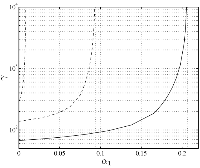
Figure 4: The minimum norm versus $\alpha_{1}$ for $s_{1}=[1~{}0~{}0]$ (dash-dot), $s_{1}=[1~{}1~{}0]$ (dashed), and $s_{1}=[1~{}1~{}1]$ (solid)

In the second part of simulations, we assumed a channel only on the actuator side with the switching pattern $s_{2}=[1~{}0]$ and perfect communication on the sensor side. We designed dynamic controllers of the form (5) for three cases: State feedback, output feedback, and output feedback with the zero-order hold type decoder (i.e., it functions as a one-step delay). In these cases, the upper bound on $\alpha_{2}$ is $1/(\lambda_{1}\cdot\lambda_{2})^{4}=0.0427$ by the results in Section 4. We note that the dimension of the controller is different for the one with the decoder since it was designed for the generalized plant including the decoder.

For each $\alpha_{2}$, the minimum $H^{\infty}$ norm for the closed-loop system was calculated. The results are plotted in Fig. 5. The norms indeed explode as $\alpha_{2}$ approach the upper bound. It is interesting to note that, for this example, the performance of the system with the decoder is worse especially for large $\alpha_{2}$. This may be explained as follows: As $\alpha_{2}$ becomes larger, so does the feedback gain, and hence the chance to apply a wrong control is higher.

6 Conclusion

In this paper, we have considered the problem of stabilization of a linear system over shared and unreliable channels. We have shown that there are critical probability values for the losses above which stability cannot be achieved. The implication is the tradeoff between control performance and transmission rate for the communication. The approach is based on the $H^{\infty}$ design method proposed in [12].

Acknowledgement:  This work was supported in part by the Ministry of Education, Culture, Sports, Science and Technology, Japan, under Grant No. 17760344.

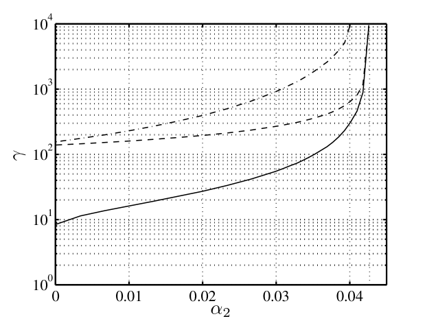
Figure 5: The minimum norm versus $\alpha_{2}$ for state feedback (solid), output feedback (dashed), and output feedback with a decoder (dash-dot)

Appendix A Appendix

We provide the proof of Proposition 4.1. This proof consists of two steps. The next lemma is the key to relate the state feedback problem to another problem arising in $H^{\infty}$ control.

Lemma A.1

The following are equivalent:

1. The closed-loop system of (6) and (8) is stochastically stable.

2. There exists a positive-definite matrix $P\in{\mathbb{R}}^{n\times n}$ and a gain $F\in{\mathbb{R}}^{1\times n}$ such that

   $$\alpha_{2}A^{T}PA+(1-\alpha_{2})(A+BF)^{T}P(A+BF)-P<0.$$ (23)

3. There exists a positive-definite matrix $P\in{\mathbb{R}}^{n\times n}$ such that

   $$\begin{split}&A^{T}PA-P-A^{T}PB\left(\frac{1}{1-\alpha_{2}}+B^{T}PB\right)^{-1}B^{T}PA<0,\\ &\frac{1}{\alpha_{2}}-B^{T}PB>0.\end{split}$$ (24)

4. There exists a state feedback gain $F$ such that

   $$\left\|F(zI-A-BF)^{-1}B\right\|<\frac{1}{\sqrt{\alpha_{2}}},$$

   where $\lVert\cdot\rVert$ is the $H^{\infty}$ norm of a transfer function.

Furthermore, if the condition (iii) holds for some $P$, then the inequality (23) in (ii) holds with the same $P$ and the gain $F$ given by

$$F=-\left(B^{T}PB\right)^{-1}B^{T}PA.$$

Proof :  The equivalence between (i) and (ii) is a direct consequence of Lemma 2.1. We next show that (ii) holds if and only if (iii) does. The inequality (23) in (ii) is equivalent to the following one:

$$A^{T}PA-P+(1-\alpha_{2})\left(F+(B^{T}PB)^{-1}B^{T}PA\right)^{T}B^{T}PB\left(F+(B^{T}PB)^{-1}B^{T}PA\right)$$

$$\hskip 170.71652pt\mbox{}-(1-\alpha_{2})A^{T}PB(B^{T}PB)^{-1}B^{T}PA<0.$$ (25)

This is shown by expanding (23) and then completing the square for $F$. Hence, (ii) is equivalent to the existence of $P>0$ such that

$$A^{T}PA-P-(1-\alpha_{2})A^{T}PB(B^{T}PB)^{-1}B^{T}PA<0.$$ (26)

Now, suppose that (ii) holds, that is, the inequality (26) above holds. This inequality can be expressed as

$$A^{T}PA-P-A^{T}PB\left(\frac{\alpha_{2}}{1-\alpha_{2}}B^{T}PB+B^{T}PB\right)^{-1}B^{T}PA<0.$$

We also note that the inequality (23) holds for any scaling $\mu P$ of $P$ with positive real $\mu$. Thus, there exists $\mu$ such that $\mu<(\alpha_{2}B^{T}PB)^{-1}$, but sufficiently close to $(\alpha_{2}B^{T}PB)^{-1}$ that satisfies

$$A^{T}\mu PA-\mu P-A^{T}\mu PB\left(\frac{1}{1-\alpha_{2}}+B^{T}\mu PB\right)^{-1}B^{T}\mu PA<0.$$

Therefore, for $\mu P$, the inequalities (24) in (iii) hold.

To show the converse, observe that the second inequality in (24) implies

$$(1-\alpha_{2})\left(B^{T}PB\right)^{-1}>\left(\frac{1}{1-\alpha_{2}}+B^{T}PB\right)^{-1}.$$

Hence, for $P$ satisfying (24) in (iii), the inequality (26) also holds. This implies (ii). Moreover, the last statement of the lemma holds true since, in view of (25), $P$ and the gain $F=-(B^{T}PB)^{-1}B^{T}PA$ satisfy the inequality (23).

The equivalence between (iii) and (iv) can be shown using the standard $H^{\infty}$ control theory; see, e.g., [1]. $\square$

The $H^{\infty}$ control problem in (iii) in the lemma has appeared in the context of quantized control with logarithmic quantizers [5, 6]. The following result is from [6, Lemma 2.4], which provides an analytic bound for the problem.

Lemma A.2

$$\inf_{F}\left\|F(zI-A-BF)^{-1}B\right\|=\prod_{\lvert\lambda_{i}\rvert>1}\lvert\lambda_{i}\rvert,$$

where the infimum is taken over $F$ such that $A+BF$ is stable.

The proof of Proposition 4.1 now follows immediately from Lemmas A.1 and A.2. We note that Lemma A.1 provides a method to design the feedback gain $F$ for each $\alpha_{2}$ satisfying the bound (9).

References

- [1] T. Başar and P. Bernhard. -Optimal Control and Related Minimax Design Problems: A Dynamic Game Approach, 2nd edition. Birkhäuser, Boston, 1995.
- [2] O. L. V. Costa and M. D. Fragoso. Stability results for discrete-time linear systems with Markovian jumping parameters. J. Math. Anal. Applicat., 179:154–178, 1993.
- [3] N. Elia. Remote stabilization over fading channels. Systems & Control Letters, 54:238–249, 2005.
- [4] N. Elia and J. N. Eisenbeis. Limitations of linear remote control over packet drop networks. In Proc. 43rd IEEE Conf. on Decision and Control, pages 5152–5157, 2004.
- [5] N. Elia and S. K. Mitter. Stabilization of linear systems with limited information. IEEE Trans. Autom. Control, 46:1384–1400, 2001.
- [6] M. Fu and L. Xie. The sector bound approach to quantized feedback control. IEEE Trans. Autom. Control, 50:1698–1711, 2005.
- [7] V. Gupta, B. Hassibi, and R. M. Murray. Optimal lqg control across packet-dropping links. Systems & Control Letters, 56:439–446, 2007.
- [8] C. N. Hadjicostis and R. Touri. Feedback control utilizing packet dropping network links. In Proc. 41st IEEE Conf. on Decision and Control, pages 1205–1210, 2002.
- [9] D. Hristu and K. Morgansen. Limited communication control. Systems & Control Letters, 37:193–205, 1999.
- [10] O. Ç. Imer, S. Yüksel, and T. Başar. Optimal control of LTI systems over unreliable communication links. Automatica, 42:1429–1439, 2006.
- [11] H. Ishii. Stabilization under shared communication with message losses and its limitations. In Proc. 45th IEEE Conf. on Decision and Control, pages 4974–4979, 2006.
- [12] H. Ishii. control with limited communication and message losses. Systems & Control Letters, 57:322–331, 2008.
- [13] H. Ishii. On the feedback information in stabilization over unreliable channels. In Proc. 17th IFAC World Congress, to appear, 2008.
- [14] H. Ishii and B. A. Francis. Limited Data Rate in Control Systems with Networks, volume 275 of Lect. Notes Contr. Info. Sci. Springer, Berlin, 2002.
- [15] H. Ishii and S. Hara. A subband coding approach to control under limited data rates and message losses. Automatica, 44:1141–1148, 2008.
- [16] Y. Ji and H. J. Chizeck. Jump linear quadratic Gaussian control: Steady-state solution and testable conditions. Control Theory Adv. Technol., 6:289–319, 1990.
- [17] T. Katayama. On the matrix Riccati equation for linear systems with random gain. IEEE Trans. Autom. Control, 21:770–771, 1976.
- [18] L. Lu, L. Xie, and M. Fu. Optimal control of networked systems with limited communication: A combined heuristic and convex optimization approach. In Proc. 42nd IEEE Conf. on Decision and Control, pages 1194–1199, 2003.
- [19] S. Mastellone, C. T. Abdallah, and P. Dorato. Model-based networked control for nonlinear systems with stochastic packet dropout. In Proc. American Control Conf., pages 2365–2370, 2005.
- [20] P. Seiler and R. Sengupta. An approach to networked control. IEEE Trans. Autom. Control, 50:356–364, 2005.
- [21] B. Sinopoli, L. Schenato, M. Franceschetti, K. Poolla, M. I. Jordan, and S. S. Sastry. Kalman filtering with intermittent observations. IEEE Trans. Autom. Control, 49:1453–1464, 2004.
- [22] B. Sinopoli, L. Schenato, M. Franceschetti, K. Poolla, and S. S. Sastry. An LQG optimal linear controller for control systems with packet losses. In Proc. 44th IEEE Conf. on Decision and Control and European Control Conf., pages 458–463, 2005.
- [23] Y. Xu and J. P. Hespanha. Estimation under uncontrolled and controlled communications in networked control systems. In Proc. 44th IEEE Conf. on Decision and Control and European Control Conf., pages 842–847, 2005.