Solitons in Bose-Einstein Condensates with time-dependent atomic scattering length in an expulsive parabolic and complex potential

Abstract

We present two families of analytical solutions of the one-dimensional nonlinear Schrödinger equation which describe the dynamics of bright and dark solitons in Bose-Einstein condensates (BECs) with the time-dependent interatomic interaction in an expulsive parabolic and complex potential. We also demonstrate that the lifetime of both a bright soliton and a dark soliton in BECs can be extended by reducing both the ratio of the axial oscillation frequency to radial oscillation frequency and the loss of atoms. It is interested that a train of bright solitons may be excited with a strong enough background. An experimental protocol is further designed for observing this phenomenon.

I Introduction

The Bose-Einstein condensates (BECs) at nK temperature can be described by the mean field theory – nonlinear Schrödinger (NLS) equation with a trap potential, i.e., the Gross-Pitaevskii (GP) equation. Recently, with the experimental observation and theoretical studies of BECs rmp71(1999)463 , there has been intense interest in the nonlinear excitations of ultra-cold atoms, such as dark solitons prl83(1999)5198 ; science287(2000)97 ; prl84(2000)2298 ; prl85(2000)1598 ; prl86(2001)2926 ; bwu-prl98(2002)034101 , bright solitons Nature417(2002)150 ; prl90(2003)230401 ; Science296(2002)1290 , vortices prl83(1999)2498 and the four-wave mixing Nature398(1999)218 . Recent experiments have demonstrated that the variation of the effective scattering length, even including its sign, can be achieved by utilizing the so-called Feshbach resonance prl82(1999)2422 ; prl81(1998)5109 ; nature392(1998)151 . It has been demonstrated that the variation of nonlinearity of the GP equation via Feshbach resonance provides a powerful tool for controlling the generation of bright and dark soliton trains starting from periodic waves prl90(2003)230402 .

At the mean-field level, the GP equation governs the evolution of the macroscopic wave function of BECs. In the physically important case of the cigar-shaped BECs, it is reasonable to reduce the GP equation into a one-dimension nonlinear Schrödinger equation with time-dependent atomic scattering length in an expulsive parabolic and complex potential pra57(1998)3837 ; mplb18(2004)173 ; prl94(2005)050402 ; prl92(2004)220403 ; mplb18(2004)627 ; jpb39(2006)3679 ,

$${\rm i}\frac{\partial\psi}{\partial t}=-\frac{\partial^{2}\psi}{\partial x^{2}}+2a(t)|\psi|^{2}\psi-\frac{1}{4}\lambda^{2}x^{2}\psi+{\rm i}\gamma\psi,$$ (1)

where the time $t$ and coordinate $x$ are measured in units $2/\omega_{\perp}$ and $a_{\perp}$, $a_{\perp}=\sqrt{\hbar/m\omega_{\perp}}$ and $a_{0}=\sqrt{\hbar/m\omega_{0}}$ are linear oscillator lengths in the transverse and cigar-axis directions, respectively. $\omega_{\perp}$ is the radial oscillation frequency and $\omega_{0}$ is the axial oscillation frequency. $m$ is the atomic mass, $|\lambda|=2|\omega_{0}|/\omega_{\perp}\ll 1$, $a(t)$ is a scattering length of attractive interactions ($a(t)<0$) or repulsive interactions ($a(t)>0$) between atoms, and $\gamma$ is a small parameter related to the feeding of condensate from the thermal cloud prl81(1998)933 . When $a(t)=g_{0}\exp(\lambda t)$ and $\gamma=0$, Liang et al. present a family of exact solutions of (1) by Darboux transformation and analyze the dynamics of a bright soliton prl94(2005)050402 . Kengne et al. investigated (1) with $a(t)=g_{0}$ and $\gamma=\lambda/2$ and verified the dynamics of a bright soliton proposed jpb39(2006)3679 . These results show that, under a safe range of parameters, the bright soliton can be compressed into very high local matter densities by increasing the absolute value of the atomic scattering length or feeding parameter.

In this paper, we develop a direct method to derive two families of exact solitons of Eq. (1), then give some thorough analysis for a bright soliton, a train of bright solitons and a dark soliton. Our results show that for BEC system with time-dependent atomic scattering length, the lifetime of a bright or a dark soliton in BECs can keep longer times by reducing both the ratio of the axial oscillation frequency to radial oscillation frequency and the loss of atoms. It is demonstrated that a train of bright solitons in BECs may be excited with a strong enough background. We also propose an experimental protocol to observe this phenomenon in further experiments.

II The Method and Soliton Solutions

We can assume the solutions of Eq. (1) as follows

$$\psi=[A_{{0}}(t)+A_{{1}}(t){\frac{\delta\,\cosh(\xi)+\cos(\eta)}{\cosh(\xi)+\delta\,\cos(\eta)}}+{{\rm i}B_{{1}}(t)\frac{\alpha\,\sinh(\xi)+\beta\,\sin(\eta)}{\cosh(\xi)+\delta\,\cos(\eta)}}]\exp({\rm i}\Delta),$$ (2)

where

$$\Delta=k_{{0}}(t)+k_{{1}}(t)x+k_{{2}}(t){x}^{2},\ \ \xi=p_{{1}}(t)x+q_{{1}}(t),\ \ \eta=p_{{2}}(t)x+q_{{2}}(t),$$

and $A_{0}(t)$, $A_{1}(t)$, $B_{1}(t)$, $p_{1}(t)$, $q_{1}(t)$, $p_{2}(t)$, $q_{2}(t)$, $k_{0}(t)$, $k_{1}(t)$, $k_{2}(t)$ are real functions of $t$ to be determined, and $\alpha,\beta,\delta$ are real constants.

Substituting Eq. (2) into Eq. (1), we first remove the exponential terms, then collect coefficients of $\sinh^{i}(\xi)\cosh^{j}(\xi)\sin^{m}(\eta)\cos^{n}(\eta)x^{k}$ ($i=0,1,2,\cdots$; $j=0,1$; $m=0,1,2,\cdots$; $n=0,1$; $k=0,1,\cdots.$) and separate real part and imaginary part for each coefficient. We derive a set of ordinary differential equations (ODEs) with respect to $a(t)$, $A_{0}(t)$, $A_{1}(t)$, $B_{1}(t)$, $p_{1}(t)$, $q_{1}(t)$, $p_{2}(t)$, $q_{2}(t)$, $k_{0}(t)$, $k_{1}(t)$, $k_{2}(t)$. Finally, solving these ODEs, we can obtain two families of analytical solutions of Eq. (1).

Family 1. When interaction between atoms is attractive such as ⁷Li atoms, $a(t)<0$, the solution of Eq. (1) can be written as:

$$\psi_{1}=\Omega[A_{c}+A_{s}{\frac{(\delta\,\cosh(\xi)+\cos(\eta))}{\cosh(\xi)+\delta\,\cos(\eta)}}+{\rm i}A_{s}{\frac{\alpha\,\sinh(\xi)+\beta\,\sin(\eta)}{\cosh(\xi)+\delta\,\cos(\eta)}}]\exp({\rm i}\Delta+\gamma t),$$ (3)

where

$$\Delta = k_{2}(t)x^{2}+k_{1}\Omega^{2}x+(2g_{0}A_{c}^{2}-k_{1}^{2})\int\!\!\Omega^{4}{\rm d}t,$$

$$\xi = \!\!\sqrt{g_{0}}A_{s}[\beta\Omega^{2}x-\!\!2[k_{1}\beta+p_{2}\!\!-\frac{2g_{0}p_{2}A_{c}^{2}}{(g_{0}A_{s}^{2}+p_{2}^{2})}]\!\!\int\!\!\Omega^{4}{\rm d}t],$$

$$\eta = p_{2}\Omega^{2}x-[2p_{2}k_{1}+(p_{2}^{2}-g_{0}A_{s}^{2})\beta]\int\!\Omega^{4}{\rm d}t,$$

$$a(t) = -g_{0}\Omega^{2}\exp(-2\gamma t),\ \ \alpha=-\frac{2\sqrt{g_{0}}A_{c}p_{2}}{g_{0}A_{s}^{2}+p_{2}^{2}},$$

$$\beta^{2} = \frac{p_{2}^{2}+g_{0}(A_{s}^{2}-4A_{c}^{2})}{g_{0}A_{s}^{2}+p_{2}^{2}},\ \ \delta=-\frac{2g_{0}A_{c}A_{s}}{g_{0}A_{s}^{2}+p_{2}^{2}},$$

$$\Omega = {\rm exp}[\int\!-2k_{2}(t){\rm d}t],\ \ k_{{2}}(t)=\{\pm\frac{\lambda}{4},\ \ \frac{\lambda}{4}{\tanh(\lambda t)}\},$$

and $A_{c},A_{s},g_{0}>0$, $p_{2}$, $k_{1}$, $\gamma$ are arbitrary real constants.

Family 2. When interaction between atoms is repulsive such as ²³Na and ⁸⁷Rb atoms, $a(t)>0$, the solution of Eq. (1) can be written as:

$$\psi_{2}=\Omega[A_{c}+iA_{s}\tanh(\xi)]\exp(i\Delta+\gamma t),$$ (4)

where

$$\xi = \pm\sqrt{g_{0}}\Omega^{2}x+2A_{s}(\sqrt{g_{0}}k_{1}+g_{0}A_{c})\int\!\Omega^{4}{\rm d}t,$$

$$\Delta = k_{2}(t)x^{2}\!+\!k_{1}\Omega^{2}x\!-\![2g_{0}(A_{c}^{2}\!+\!A_{s}^{2})\!+\!k_{1}^{2}]\int\!\!\Omega^{4}{\rm d}t,$$

$$a(t) = g_{0}\Omega^{2}\exp(-2\gamma t),$$

and $\Omega,k_{2}(t)$ are the same as in (3), $A_{c},A_{s},g_{0}>0$, $k_{1}$ and $\gamma$ are arbitrary real constants.

The solutions (3) and (4) are new general solutions of equation (1) which can describe the dynamics of bright and dark solitons in BECs with the time-dependent interatomic interaction in an expulsive parabolic and complex potential. In special case, it can be reduced to solutions obtained by others. For example, if $k_{2}(t)=-\lambda/4$ and $\gamma=0$, the solution (3) describe dynamics of a bright soliton in BECs with time-dependent atomic scattering length in an expulsive parabolic potential, and it can reduce the solution in Ref. prl94(2005)050402 . If $k_{2}(t)=-\lambda/4$ and $\gamma=\lambda/2$, Eq. (3) describe dynamics of bright matter wave solitons in BECs in an expulsive parabolic and complex potential, and it can recover the solution in Ref. jpb39(2006)3679 .

To our knowledge, the other solutions from Eqs. (3) and (4) have not been reported earlier. When $k_{2}(t)=\pm\lambda/4$ and $\gamma$ is a fixed value, the intensities of Eqs. (3) and (4) are either exponentially increasing or exponentially decreasing so the BECs phenomenon can not be stable reasonably. Thus in order to close experimental condition and compare our theoretical prediction with experimental results, we will only discuss and analyze Eqs. (3) and (4) with $k_{2}(t)=\lambda/4\tanh(\lambda t)$ and $\Omega^{2}={\rm sech}(\lambda t)/2$.

II.1 Dynamics of Bright Solitons in BECs

In the following, we are interested in two cases of Eq. (3).

(I)  When $\alpha=0$ and $p_{2}=0$, $\psi_{1}$ can be written as

$$\psi_{11}=\Omega[A_{c}+A_{s}\frac{\delta\cosh(\xi)+\cos(\eta)+{\rm i}\beta\,\sin(\eta)}{\cosh(\xi)+\delta\,\cos(\eta)}]\times\exp({\rm i}\Delta+\gamma t),$$ (5)

where $A_{s}^{2}>4A_{c}^{2}$, and

$$\xi = \sqrt{g_{0}}\beta A_{s}\Omega^{2}x-2\sqrt{g_{0}}A_{s}k_{1}\beta\int\!\!\Omega^{4}{\rm d}t,$$

$$\eta = \frac{g_{0}(A_{s}^{2}-4A_{c}^{2})}{\beta}\int\!\Omega^{4}{\rm d}t,\ \ \beta^{2}=\frac{A_{s}^{2}-4A_{c}^{2}}{A_{s}^{2}},$$

$$\Delta = k_{2}(t)x^{2}+k_{1}\Omega^{2}x+(2g_{0}A_{c}^{2}-k_{1}^{2})\int\Omega^{4}{\rm d}t,$$

$$\Omega = \sqrt{\frac{{\rm sech}(\lambda t)}{2}},\ \ \delta=-\frac{2A_{c}}{A_{s}},$$

$$a(t) = -\frac{g_{0}}{2}\rm{sech}(\lambda t){\rm exp}(-2\gamma t).$$

When $A_{s}=0$, $\psi_{11}$ reduces to the background

$$\psi_{c}=A_{c}\Omega\exp({\rm i}\Delta+\gamma t).$$ (6)

When $A_{c}=0$, $\psi_{11}$ reduces to the bright soliton

$$\psi_{s}=A_{s}\Omega{\rm sech}(\xi)\exp\left[{\rm i}\Theta+\gamma t\right],$$ (7)

where

$$\xi = \sqrt{g_{0}}A_{s}\Omega^{2}x-2\sqrt{g_{0}}A_{s}(k_{1}+p_{2})\int\Omega^{4}{\rm d}t,$$

$$\Theta = k_{2}(t)x^{2}+k_{1}\Omega^{2}x+[g_{0}A_{s}^{2}-k_{1}^{2}]\int\Omega^{4}{\rm d}t.$$

Thus $\psi_{11}$ represents a bright soliton embedded in the background. At the same time, when $A_{c}\ll A_{s}$ satisfied $4A_{c}^{2}<A_{s}^{2}$ and $\gamma$ small, the background is small within the existence of bright soliton.

Considering the dynamics of the bright soliton in the background, the length $2L$ of the spatial background must be very large compared to the scale of the soliton. In the real experiment Nature417(2002)150 , the length of the background of BECs can reach at least $2L=370{\rm\mu m}$. In Fig.1, the width of the bright soliton is about $2l=14{\rm nm}$ [a unity of coordinate, $\Delta x=1$ in the dimensionless variables, corresponds to $a_{\perp}=(\hbar/(m\omega_{\perp})^{1/2}=1.4{\rm\mu m}$]. So $l\ll L$, a necessary condition for realizing bright soliton in experiment. From Fig.1a, under the realistic experiment parameters in Science296(2002)1290 , i.e., $\omega_{\perp}=2\pi\times 710$Hz, $\omega_{0}=2{\rm i}\pi\times 70$Hz. In order to cope with the experiment: the soliton move to $-x$ direction, $\lambda=-2|\omega_{0}|/\omega_{\perp}\approx-0.197$, $\gamma=-0.01$ and $g_{0}=0.4$nm , we can see that the lifetime of the BEC is about $20\times 4.5\times 10^{-4}s=9$ms, which is close to the experiment results: the lifetime of a BEC is about 8ms. Here, by (9), we can verify that the number of atoms in the bright soliton against the background is in the range of 4635 (at $t=-10$) and 3107 (at $t=10$), which is a proper range of atoms when the soliton can be observed Science296(2002)1290 . But, when $t\in[-10,10]$, the scattering length $a(t)=-0.2{\rm sech}(0.197t)\exp(0.02t)$ varies in [$-0.20,-0.04$] nm, which is different from the experiment condition: the scattering length keeps invariable when the bright soliton in BECs propagates in the magnetic trap Science296(2002)1290 . However, up to now, they can not measure the motion of dark or bright soliton when the parameter varies continually, and they only measure a particular value of soliton corresponding to the fixed magnetic field. When we fix the magnetic field at a fixed value (the scattering length is also a fixed value) such as $B=425$G in Ref. Science296(2002)1290 , the scattering length is $a_{s}=-0.21$ nm, then the special value of our general solution is in accordance with the experimental data of Ref. Science296(2002)1290 . Of course, we believe that with the development of the Feshbach resonance technology, the experimental physicists can measure the motion of solitons in the future. Thus by modulating the scattering length in time via changing magnetic field near the Feshbach resonance, we may also realize the bright solitons in BECs.

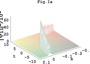
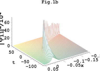
Fig. 1: (Color online) The evolution plots of $|\psi_{11}|^{2}/10^{4}$, where $A_{c}=4,A_{s}=1200,g_{0}=0.4$. In Fig.1a: $\lambda=-0.197,\gamma=k_{1}=-0.01$; In Fig.1b: $\lambda=-0.02,\gamma=k_{1}=-0.001$.

When $\lambda=-0.02$ (which can be derived from $\omega_{0}=2{\rm i}\pi\times 7$Hz and $\omega_{\perp}=2\pi\times 710$Hz) and $\gamma=-0.001$, from Fig.1b, the lifetime of the BEC can reach about 200 unities of the dimensionless time corresponds to a real time of 0.1s, which arrives at the order of the lifetime of a BEC in today’s experiments. Here, we can verify that when $t$ is from -120 to 80, (i) the number of atoms is in the range of 4824 and 3234 by (9); (ii) the scattering length $-0.20{\rm nm}\leq a(t)\leq-0.03{\rm nm}$; (iii) From (5), we can derive $\xi\approx-1/2\sqrt{g_{0}}\sqrt{A_{s}^{2}-4A_{c}^{2}}(x-k_{1}t-x_{0})$, therefore, $k_{1}$ describes the velocity of the bright soliton, which can be demonstrated by Fig. 1.

It is necessary to point out that, (i) In order to give clear figures, the parameter $k_{1}$ is taken to be relatively small. In reality, $k_{1}$ is about to $-4$, which can be derived from the soliton’s position $x=-k_{1}\exp(-\lambda t)/\lambda$; (ii) The background is very small with regard to the bright soliton in Fig. 1, which can be also shown by Fig. 2. Therefore the background may be taken as zero background approximatively; (iii) In order to keep the lifetime of the bright soliton about 8ms, we take $\gamma=-0.01$ which may be the experimental value. When $\gamma=-0.01$, by varying the value of $\lambda$, it is difficult to extend the lifetime of the bright soliton. Thus in order to extending the lifetime of a soliton in BEC, we should take appropriate measures to reduce the absolute value of $\lambda$ and $\gamma$, as is shown in Fig. 1b.

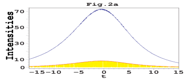
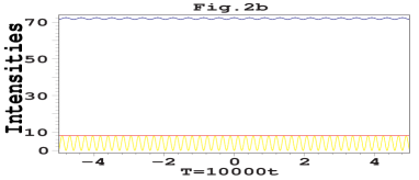
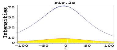
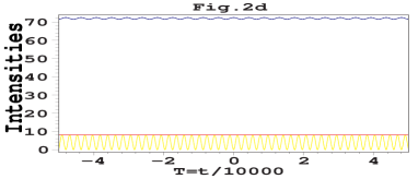
Fig. 2: (Color online) The evolution plots of $|\psi_{11}|^{2}_{\rm max}/10^{4}$ (blue line) and $|\psi_{11}|^{2}_{\rm min}$ (yellow line) and $|\psi_{c}|^{2}$ (red line). The parameters in Fig. 2a-2b and Fig. 2c-2d are the same as in Fig. 1a and Fig. 1b, respectively.

Furthermore, we find that when $\cosh(\xi)=-2A_{c}\cos(\eta)/A_{s}+A_{s}/(A_{c}\cos(\eta))$ ($\sinh(\xi)=0$), the intensity of (5) arrives at the minimum (maximum)

$$|\psi_{11}|^{2}_{\rm min} = A_{c}^{2}[1-\frac{(A_{s}^{2}-4A_{c}^{2})\cos^{2}(\eta)}{A_{s}^{2}-4A_{c}^{2}\cos^{2}(\eta)}]\frac{{\rm sech}(\lambda t)}{2}{\rm e}^{2\gamma t},$$

$$|\psi_{11}|^{2}_{{\rm max}} = [A_{c}^{2}+\frac{A_{s}(A_{s}^{2}-4A_{c}^{2})}{A_{s}-2A_{c}\cos(\eta)}]\frac{{\rm sech}(\lambda t)}{2}{\rm e}^{2\gamma t}.$$ (8)

This means that the bright solitons (5) can be only squeezed into the assumed peak matter density between the minimum and maximum values. Fig.2 present the evolution plots of the maximal and minimal intensities given by $|\psi_{11}|^{2}_{\rm max}/10^{4}$ (blue line) and $|\psi_{11}|^{2}_{\rm min}$ (yellow line) and the background intensity (red line) with different parameters. From Fig.2, with the time evolution, firstly the intensities increase until to the peak, then decrease to the background. Meanwhile, the smaller $|\lambda|$ and $|\gamma|$, the longer the higher intensities can keep. Therefore in order to keep a bright soliton in BECs for longer time, we should reduce both the ratio of the axial oscillation frequency to radial oscillation frequency and the loss of atoms.

To investigate the stability of the bright soliton in the expulsive parabolic and complex potential, we obtain

$$\int_{-L}^{+L}\!\!(|\psi_{11}|^{2}-|\psi_{c}|^{2})dx=N_{0}C_{L},$$ (9)

where

$$N_{0} = \frac{2\sqrt{A_{s}^{2}-4A_{c}^{2}}}{\sqrt{g_{0}}}\exp(2\gamma t)$$ (10)

$$C_{L} = \frac{A_{s}(\exp(2L)-1)}{A_{s}(\exp(2L)+1)-4A_{c}\cos(\eta)\exp(L)},$$ (11)

which is the exact number of the atoms in the bright soliton against the background described by (5) within $[-L,L]$. This indicates that when $L$ takes a fixed value, for example, $L=100$, then $C_{L}\rightarrow 1$, therefore the number of atoms in the bright soliton is determined by $N_{0}$.

In contrast, the quantity

$$\int_{-L}^{L}|\psi_{11}-\psi_{c}|^{2}dx=N_{0}\{C_{L}+4A_{c}M\cos(\eta)\},$$ (12)

where $N_{0}$ and $C_{l}$ are determined by (10) and (11), and

$$M = \frac{1}{\Theta}\arctan[\frac{A_{s}+2A_{c}\cos(\eta)}{\Theta}\cdot\frac{\exp(L)-1}{\exp(L)+1}],$$

$$\Theta = \sqrt{A_{s}^{2}-4A_{c}^{2}\cos^{2}(\eta)},$$

counts the number of atoms in both the bright soliton and background under the condition of $\psi(\pm L,t)\neq 0$. Equation (12) displays that a time-periodic atomic exchange is formed between the bright soliton and the background. In the case of zero background, i.e., $A_{c}=0$, from (12) the exchange of atoms depends on the sign of $\gamma$: (i) when $\gamma=0$, there will be no exchange of atoms; (ii) when $\gamma<0$, the exchange of atoms decreases; (iii) when $\gamma>0$, the exchange of atoms increases. As shown in Fig. 3, in the case of nonzero background and $\gamma<0$, a slow-fast-slow process of atomic exchange is performed between the bright soliton and the background, but the whole trend of the atomic exchange between the bright soliton and the background is decrease. In Ref. pra75(2007)037601 , Wu et al show that the number of atoms continuously injected into Bose-Einstein condensate from the reservoir depends on the linear gain/loss coefficient, and cannot be controlled by applying the external magnetic field via Feshbach resonance. The findings here can recover the same results.

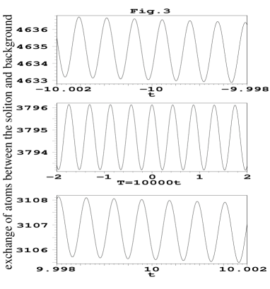
Fig. 3: (Color online) The atomic exchange between the bright solitons and the background given by (12) with $\lambda=-0.197,A_{c}=4,A_{s}=1200,g_{0}=0.4,\gamma=-0.01$.

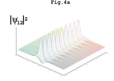
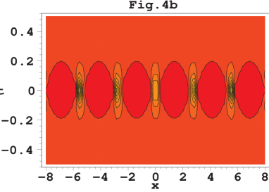
Fig. 4: (Color online) The evolution plots of $|\psi_{12}|^{2}$ with $\lambda=-0.197,A_{c}=7,A_{s}=12,g_{0}=0.4,k_{1}=-0.01,\gamma=-0.01$. Fig. 4b is the contour plot.

In addition, under the integration constant of $\int\Omega^{4}(t){\rm d}t$ taken to be zero, (5) take the following particular form at $t_{0}=\frac{1}{2\lambda}\ln[-\frac{g_{0}(A_{s}^{2}-4A_{c}^{2})}{\lambda\beta(2k+1)\pi}-1]$ $(k=0,\pm 1,\pm 2,\cdots,)$.

$$\psi_{11}=\Omega(t_{0})\left[-A_{c}\pm iA_{s}\beta{\rm sech}(\xi)\right]\exp(i\Delta+\gamma t_{0}).$$ (13)

This means that (13) can be generated by coherently adding a bright soliton into the background.

Inspired by two experiments Nature417(2002)150 ; Science296(2002)1290 , we can design an experimental protocol to control the soliton in BECs near Feshbach resonance with the following steps: (i) Create a bright soliton in BECs with the parameters of $N\approx 4\times 10^{3}$, $\omega_{\perp}=2{\rm i}\pi\times 700$Hz and $\omega_{0}=2\pi\times 7$ Hz, and for ⁷Li. (ii) Under the safe range of parameters discussed above, ramp up the absolute value of the scattering length according to $a(t)=-\frac{g_{0}}{2}\rm{sech}(\lambda t){\rm exp}(-2\gamma t)$ due to Feshbach resonance, control the dispersion of atoms in BECs at a low level by modulating the parameter $\gamma$ about to $-0.001$, and take $\lambda$ to be a very small value: $\lambda=-2|\omega_{0}|/\omega_{\perp}=-0.02$. A unity of time, $\Delta t=1$ in the dimensionless variables, corresponds to real seconds $2/\omega_{\perp}=4.5\times 10^{-4}$. (iii) During 200 dimensionless units of time, the absolute value of the atomic scattering length varies in $0.03{\rm nm}\leq|a(t)|\leq 0.20{\rm nm}$. This means that during the process of the bright soliton, the stability of soliton and the validity of 1D approximation can be kept as displayed in Fig. 1b. Therefore, the phenomena discussed in this paper should be observable within the current experimental capability.

(II) When $\beta=0$, the solution $\psi_{1}$ is written as

$$\psi_{12}=\Omega[A_{c}+A_{s}{\frac{\delta\,\cosh(\xi)+\cos(\eta)+i\alpha\,\sinh(\xi)}{\cosh(\xi)+\delta\,\cos(\eta)}}]\times\exp(i\Delta+\gamma t),$$ (14)

where $4A_{c}^{2}-A_{s}^{2}>0$ and

$$\xi = \sqrt{g_{0}}A_{s}p_{2}\int\Omega^{4}{\rm d}t,\ \ \alpha=-\frac{p_{2}}{2\sqrt{g_{0}}A_{c}},$$

$$\eta = p_{2}\Omega^{2}x-2p_{2}k_{1}\int\!\Omega^{4}{\rm d}t,\ \ \delta=-\frac{A_{s}}{2A_{c}},$$

$$p_{2}^{2} = g_{0}(4A_{c}^{2}-A_{s}^{2}),\ \ \Omega=\sqrt{\frac{{\rm sech}(\lambda t)}{2}}.$$

Analysis reveals that $\psi_{12}$ is periodic with a period $\Gamma=4\pi/[{p_{2}{\rm sech}(\lambda t)}]$ in the space coordinate $x$ and aperiodic in the temporal variable $t$. Note that the period $\Gamma$ is not a constant due to the presence of the function ${\rm sech}(\lambda t)$, but when $\lambda\ll 1$ and $t$ is very small, $\Gamma$ is very close to $4\pi/p_{2}$. As shown in Fig.4, when $\lambda=-0.197$, $A_{c}=7,A_{s}=12,g_{0}=0.4$, $k_{1}=\gamma=-0.01$, a train of bright solitons is excited. Here the atoms in a bright soliton and in the background in a period $[0,\Gamma]$ are $\int_{0}^{\Gamma}|\psi_{12}|^{2}dx\approx 3510$, $\int_{0}^{\Gamma}|A_{c}\Omega|^{2}dx\approx 6815$, respectively. Thus we can conclude that an important condition for exciting a train of bright solitons is that the background is strong enough.

II.2 Dynamics of a Dark Soliton in BECs

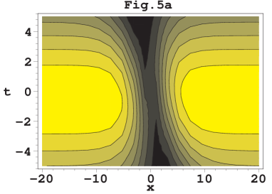
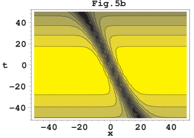
Fig. 5: (Color online) The evolution contour plots of $|\psi_{2}|^{2}$, where $A_{c}=7,A_{s}=12,g_{0}=0.4,k_{1}=-4.4$, $\lambda=-0.197$ and $\gamma=-0.01$ in Fig.5a ; $\lambda=-0.02$ $\gamma=-0.001$ in Fig.5b.

When $\lambda\rightarrow 0$ and $\gamma\rightarrow 0$, (4) is reduced to the dark soliton prl93(2004)240403 ,

$$\psi_{2}=\frac{\sqrt{{2}}}{2}[A_{c}+iA_{s}\tanh(\frac{\sqrt{g_{0}}}{2}(x+A_{s}(k_{1}+\sqrt{g_{0}}A_{c}))t)]\exp(i\Delta).$$ (15)

Therefore, the solution (4) should be a time-dependent dark soliton, which can be shown by Fig. 5. From (4), we can obtain the intensities of the background as follows

$$|\psi_{c}|^{2}=(A_{c}^{2}+A_{s}^{2})\frac{{\rm sech}(\lambda t)}{2}\exp(2\gamma t).$$ (16)

Therefore from (16), we guess that the solution (4) may describe an interesting physical process: there are ”moving stop”, which may be realized by use of laser, at both ends of the cigar-axis direction.

Proceeding as the case of the bright soliton, we obtain

$$\int_{-\infty}^{+\infty}|\psi_{2}|^{2}-|\psi_{2}(\pm\infty,t)|^{2}{\rm d}x=-\frac{2A_{s}^{2}}{\sqrt{g_{0}}}\exp(2\gamma t),$$ (17)

which describes the region of decreased density and contains a negative ”number of atoms”.

As shown in Fig.5, when the absolute of $\lambda$ and $\gamma$ are smaller, the dark solitons can keep a longer time and propagate a longer distance. Under the conditions in Fig.5, the scattering lengths are in a range $0.05{\rm nm}\leq a(t)\leq 0.20{\rm nm}$. Therefore in order to keep a dark soliton a long time in BECs, we should also reduce the values of $\lambda$ by adjusting the harmonic oscillator frequencies $\omega_{\perp}$ and $\omega_{0}$ and reduce the absolute value of $\gamma$ by controlling the loss of atoms.

III Conclusions

In summary, we present a direct method to obtain two families of analytical solutions for the nonlinear Schrodinger equation which describe the dynamics of solitons in Bose-Einstein condensates with the time-dependent interatomic interaction in an expulsive parabolic and complex potential. The dynamics of a bright soliton, a train of bright solitons and a dark soliton are analyzed thoroughly. We can extend the lifetime of a bright soliton or a dark soliton in BEC by reducing the ratio of the axial oscillation frequency to radial oscillation frequency and control the loss of atoms. Meanwhile, our results also demonstrate that a train of bright solitons in BEC may be excited with a strong enough background. It is very interesting to find these new phenomena which are of special importance in the field of an atom laser in further experiments.

B. Li would express his sincerely thanks to Profs. G. X. Huang and Z. D. Li for their helpful discussions. This work is supported by the NSF of China under Grant Nos. 10747141, 10735030, 90406017, 60525417, 10740420252, the NKBRSF of China under Grant 2005CB724508, 2006CB921400, Zhejiang Provincial NSF of China under Grant Nos. 605408, Ningbo NSF under Grant Nos. 2007A610049, 2006A610093 and K.C.Wong Magna Fund in Ningbo University.

References

- (1) F. Dalfovo, S. Giorgini, L. P. Pitaevskii, and S. Stringari, Rev. Mod. Phys. 71, 463 (1999).
- (2) S. Burger, K. Bongs, S. Dettmer, W. Ertmer, K. Sengstock, A. Sanpera, G. V. Shlyapnikov, and M. Lewenstein, Phys. Rev. Lett. 83, 5198 (1999).
- (3) J. Denschlag, J. E. Simsarian, D. L. Feder, C. W. Clark, L. A. Collins, J. Cubizolles, L. Deng, E. W. Hagley, K. Helmerson, W. P. Reinhardt, S. L. Rolston, B. I. Schneider, and W. D. Phillips, Science 287, 97 (2000).
- (4) Th. Busch and J. R. Anglin, Phys. Rev. Lett. 84, 2298 (2000).
- (5) C. K. Law, C. M. Chan, P. T. Leung, and M. C. Chu, Phys. Rev. Lett. 85, 1598 (2000).
- (6) B. P. Anderson, P. C. Haljan, C. A. Regal, D. L. Feder, L. A. Collins, C.W. Clark, and E. A. Cornell, Phys. Rev. Lett. 86, 2926 (2001).
- (7) B. Wu, J. Liu, and Q. Niu, Phys. Rev. Lett. 88, 034101 (2002).
- (8) K. E. Strecker, G. B. Partridge, A. G. Truscott, and R. G. Hulet, Nature (London) 417, 150 (2002).
- (9) P. G. Kevrekidis, G. Theocharis, D. J. Frantzeskakis, and B. A. Malomed, Phys. Rev. Lett. 90, 230401 (2003).
- (10) L. Khaykovich, F. Schreck, G. Ferrari, T. Bourdel, J. Cubizolles, L. D. Carr, Y. Castin, and C. Salomon, Science 296, 1290 (2002).
- (11) M. R. Mattews, B. P. Anderson, P. C. Haljan, D. S. Hall, C. E. Wieman, and E. A. Cornell, Phys. Rev. Lett. 83, 2498 (1999).
- (12) L. Deng, E. W. Hagley, J. Wen, M. Trippenbach, Y. Band, P. S. Julienne, J. E. Simsarian, K. Helmerson, S. L. Rolston, and W. D. Phillips, Nature 398, 218 (1999).
- (13) J. Stenger, S. Inouye, M. R. Andrews, H.-J. Miesner, D. M. Stamper-Kurn, and W. Ketterle, Phys. Rev. Lett. 82, 2422 (1999).
-
(14)
J. L. Roberts, N. R. Claussen, J. P. Burke, Jr.,
C. H. Greene, E. A. Cornell, and C. E. Wieman, Phys. Rev. Lett. 81, 5109
(1998);
S. L. Cornish, N. R. Claussen, J. L. Roberts, E. A. Cornell, and C. E. Wieman, Phys. Rev. Lett. 85, 1795 (2000). - (15) S. Inouye, M. R. Andrews, J. Stenger, H.-J. Miesner, D. M. Stamper-Kurn, and W. Ketterle, nature (London) 392, 151 (1998).
- (16) F. Kh. Abdullaev, A.M. Kamchatnov, V.V. Konotop, and V. A. Brazhnyi, Phys. Rev. Lett. 90, 230402 (2003).
-
(17)
Z. X. Liang, Z. D. Zhang and W. M. Liu,
Phys. Rev. Lett. 94, 050402 (2005);
X. F. Zhang, Q. Yang, J. F. Zhang, X. Z. Chen, and W. M. Liu, Phys. Rev. A 77, 023613 (2008). - (18) E. Kengne and P. K. Talla, J. Phys. B 39, 3679 (2006).
- (19) P. G. Kevrekidis and D. J. Frantzeskakis, Mod. Phys. Lett. B 18, 173 (2004).
- (20) V. M. Perez-Garcia, V. V. Konotop, and V. A. Brazhnyi, Phys. Rev. Lett. 92, 220403 (2004).
-
(21)
V. M. Perez-Garcia, H. Michinel, and H. Herrero, Phys. Rev. A 57, 3837 (1998);
K. D. Moll, A. L. Gaeta, and G. Fibich, Phys. Rev. Lett. 90, 203902 (2003). - (22) V. A. Brazhnyi, and V. V. KONOTOP., Mod. Phys. Lett. B 18, 627 (2004).
- (23) Y. Kagan,A. E. Muryshev, and G. V. Shlyapnikov, Phys. Rev. Lett. 81, 933 (1998).
- (24) L. Wu, R. J. Jiang, Y. H. Pei, and J. F. Zhang, Phys. Rev. A 75, 037601 (2007).
- (25) V. V. Konotop and L. Pitaevskii, Phys. Rev. Lett. 93, 240403 (2004).