Slowest relaxation mode of the partially asymmetric exclusion process with open boundaries

Abstract

We analyze the Bethe ansatz equations describing the complete spectrum of the transition matrix of the partially asymmetric exclusion process on a finite lattice and with the most general open boundary conditions. We extend results obtained recently for totally asymmetric diffusion [J. de Gier and F.H.L. Essler, J. Stat. Mech. P12011 (2006)] to the case of partial asymmetry. We determine the finite-size scaling of the spectral gap, which characterizes the approach to stationarity at late times, in the low and high density regimes and on the coexistence line. We observe boundary induced crossovers and discuss possible interpretations of our results in terms of effective domain wall theories.

1 Introduction

The partially asymmetric simple exclusion process (PASEP) [1, 2] is one of the most thoroughly studied models of non-equilibrium statistical mechanics [3, 4, 5, 6]. It is a microscopic model of a driven system [7] describing the asymmetric diffusion of hard-core particles along a one-dimensional chain with $L$ sites. At late times the PASEP exhibits a relaxation towards a non-equilibrium stationary state. In the presence of two boundaries at which particles are injected and extracted with given rates, the bulk behaviour at stationarity is strongly dependent on the injection and extraction rates. The corresponding phase diagram as well as various physical quantities have been determined by exact methods [3, 4, 8, 9, 10, 11, 12, 13, 6].

Given the behaviour in the stationary state an obvious question is how the system relaxes to this state at late times. For the PASEP on a ring, where particle number is conserved, such results were obtained by means of Bethe’s ansatz some time ago [14, 15, 16]. More recently there has been considerable progress in analyzing the dynamics in the limit of totally asymmetric exclusion and on an infinite lattice, see e.g. [17, 18, 19, 20, 21, 22], where random matrix techniques can be used.

For the finite system with open boundaries there have been several studies of dynamical properties by means of numerical, phenomenological and renormalization group methods [23, 24, 25, 26, 27, 28]. For the case of symmetric diffusion a Bethe ansatz solution was constructed in [29]. Recently, we have applied Bethe’s ansatz to the PASEP with open boundaries [30, 31]. It is well-known that the PASEP can be mapped onto the spin-1/2 anisotropic Heisenberg chain with general (integrable) open boundary conditions [10, 11]. By building on recent progress in applying Bethe’s ansatz to the latter problem [32, 33, 34, 35, 36, 37] we determined the Bethe ansatz equations for the PASEP with the most general open boundary conditions. By analyzing these equations we derived the finite size scaling behaviour of the spectrum of low-lying excited states for the cases of symmetric and totally asymmetric diffusion. Upon varying the boundary rates, we observed crossovers in massive regions, with dynamic exponents $z=0$, and between massive and scaling regions with diffusive ($z=2$) and KPZ ($z=3/2$) behaviour.

In the present work we extend these results to the case of partially asymmetric diffusion, where the analysis of the spectrum is significantly more involved.

Figure 1: Transition rates for the partially asymmetric exclusion process.

We now turn to a description of the dynamical rules defining the PASEP on a one dimensional lattice with $L$ sites. At any given time $t$ each site is either occupied by a particle or empty. The system is then updated as follows. In the bulk of the system, i.e. sites $i=2,\ldots,L-1$, a particle attempts to hop one site to the right with rate $p$ and one site to the left with rate $q$. The hop is prohibited if the neighbouring site is occupied. On the first and last sites these rules are modified. If site $i=1$ is empty, a particle may enter the system with rate $\alpha$. If on the other hand site $1$ is occupied by a particle, the latter will leave the system with rate $\gamma$. Similarly, at $i=L$ particles are injected and extracted with rates $\delta$ and $\beta$ respectively.

It is customary to associate a Boolean variable $\tau_{i}$ with every site, indicating whether a particle is present ($\tau_{i}=1$) or not ($\tau_{i}=0$) at site $i$. Let $|0\rangle$ and $|1\rangle$ denote the standard basis vectors in $\mathbb{C}^{2}$. A state of the system at time $t$ is then characterized by the probability distribution

$$|P(t)\rangle=\sum_{\bm{\tau}}P(\bm{\tau}|t)|\bm{\tau}\rangle,$$ (1.1)

where

$$|\bm{\tau}\rangle=|\tau_{1},\ldots,\tau_{L}\rangle=\bigotimes_{i=1}^{L}|\tau_{i}\rangle.$$ (1.2)

The time evolution of $|P(t)\rangle$ is governed by the aforementioned rules, which gives rise to the master equation

$$\frac{{\rm d}}{{\rm d}t}|P(t)\rangle = M|P(t)\rangle,$$ (1.3)

where the PASEP transition matrix $M$ consists of two-body interactions only and is given by

$$M=\sum_{k=1}^{L-1}I^{(k-1)}\otimes\widetilde{M}\otimes I^{(L-k-1)}+m_{1}\otimes I^{(L-1)}+I^{(L-1)}\otimes m_{L}.$$ (1.4)

Here $I^{(k)}$ is the identity matrix on the k-fold tensor product of $\mathbb{C}^{2}$ and $\widetilde{M}:\mathbb{C}^{2}\otimes\mathbb{C}^{2}\rightarrow\mathbb{C}^{2}\otimes\mathbb{C}^{2}$ is given by

$$\widetilde{M}=\left(\matrix{0&0&0&0\cr 0&-q&p&0\cr 0&q&-p&0\cr 0&0&0&0}\right).$$ (1.5)

The terms involving $m_{1}$ and $m_{L}$ describe injection (extraction) of particles with rates $\alpha$ and $\delta$ ($\gamma$ and $\beta$) at sites $1$ and $L$ respectively. Their explicit forms are

$$m_{1}=\left(\matrix{-\alpha&\gamma\cr\alpha&-\gamma\cr}\right),\qquad m_{L}=\left(\matrix{-\delta&\beta\cr\delta&-\beta\cr}\right).$$ (1.6)

The transition matrix $M$ has a unique stationary state corresponding to the eigenvalue zero. For positive rates, all other eigenvalues of $M$ have non-positive real parts. The late time behaviour of the PASEP is dominated by the eigenstates of $M$ with the largest real parts of the corresponding eigenvalues, as follows from the following argument. The average of an observable $X$ is given by (see e.g. Ref. [38])

$$\langle X\rangle(t)=\langle 0|X{\rm e}^{Mt}|P_{0}\rangle$$ (1.7)

Here $P_{0}$ is an initial state and $\langle 0|$ is the left eigenstate of $M$ with eigenvalue 0. This may be written in the spectral representation with respect to the eigenstates of $M$

$$\langle X\rangle(t)=\sum_{n}\langle 0|X|n\rangle{\rm e}^{\mathcal{E}_{n}t}a_{n},$$ (1.8)

where $|P_{0}\rangle=\sum_{n}a_{n}|n\rangle$ and $M|n\rangle=\mathcal{E}_{n}|n\rangle$. In the limit $t\to\infty$ only the stationary state survives and we have

$$\lim_{t\to\infty}\langle X\rangle(t)=\langle 0|X|0\rangle a_{0}.$$ (1.9)

At very late times we have

$$\langle X\rangle(t)\approx\langle 0|X|0\rangle a_{0}+\langle 0|X|1\rangle a_{1}e^{\mathcal{E}_{1}t},$$ (1.10)

where ${\mathcal{E}}_{1}$ is the eigenvalue of $M$ with the largest real part that contributes to the spectral decomposition of the initial state $|P_{0}\rangle$. Hence the relaxation rate $-\mathcal{E}_{1}$ determines the approach to the stationary state at asymptotically late times. In the next sections we determine the eigenvalue of $M$ with the largest non-zero real part using Bethe’s ansatz. The latter reduces the problem of determining the spectrum of $M$ to solving a system of coupled polynomial equations of degree $3L-1$. Using these equations, the spectrum of $M$ can be studied numerically for very large $L$, and, as we will show, analytic results can be obtained in the limit $L\rightarrow\infty$.

2 Bethe ansatz equations

In [30, 31] it was shown that the PASEP transition matrix $M$ can be diagonalised using the Bethe Ansatz. In [31] the Bethe equations were analyzed in some detail for the case $q=\gamma=\delta=0$ corresponding to totally asymmetric diffusion (TASEP). The resulting TASEP dynamical phase diagram displays interesting crossovers within the low and high density phases, at which the transition matrix eigenvalue corresponding to the slowest relaxation mode changes non-analytically.

This work is concerned with the generalization of some of these results to the PASEP case with $q,\gamma,\delta\neq 0$. Before turning to the technical details of our analysis we present a summary of our main results. Throughout this work we set without loss of generality $q<p=1$. For simplicity we only consider $L$ even, as for odd $L$ the details will be somewhat different.

As was shown in [30, 31], all eigenvalues ${\cal E}$ of $M$ can be expressed in terms of the roots $z_{j}$ of a set of $L-1$ non-linear algebraic equations as

$${\cal E}=-\mathcal{E}_{0}-\sum_{j=1}^{L-1}\frac{\left(q-1\right)^{2}z_{j}}{(1-z_{j})(qz_{j}-1)},$$ (2.1)

where

$$\mathcal{E}_{0}=\alpha+\beta+\gamma+\delta.$$ (2.2)

The complex roots $z_{j}$ satisfy the Bethe ansatz equations

$$\left[\frac{qz_{j}-1}{1-z_{j}}\right]^{2L}K(z_{j})=\prod_{l\neq j}^{L-1}\frac{qz_{j}-z_{l}}{z_{j}-qz_{l}}\frac{q^{2}z_{j}z_{l}-1}{z_{j}z_{l}-1},\ j=1\ldots L-1.$$

(2.3)

Here $K(z)=\tilde{K}(z,\alpha,\gamma)\tilde{K}(z,\beta,\delta)$, where

$$\tilde{K}(z,\alpha,\gamma)=\frac{(z+\kappa^{+}_{\alpha,\gamma})(z+\kappa^{-}_{\alpha,\gamma})}{(q\kappa^{+}_{\alpha,\gamma}z+1)(q\kappa^{-}_{\alpha,\gamma}z+1)},$$ (2.4)

and

$$\kappa^{\pm}_{\alpha,\gamma} = \frac{1}{2\alpha}\left(v_{\alpha,\gamma}\pm\sqrt{v_{\alpha,\gamma}^{2}+4\alpha\gamma}\right),$$ (2.5)

$$v_{\alpha,\gamma} = 1-q-\alpha+\gamma.$$ (2.6)

In order to ease notations we will use the following abbreviations,

$$a=\kappa^{+}_{\alpha,\gamma},\quad b=\kappa^{+}_{\beta,\delta},\quad c=\kappa^{-}_{\alpha,\gamma},\quad d=\kappa^{-}_{\beta,\delta}.$$ (2.7)

The constant $\mathcal{E}_{0}$ is expressed in our new notations as

$$\mathcal{E}_{0}=(1-q)\left(\frac{1-ac}{(1+a)(1+c)}+\frac{1-bd}{(1+b)(1+d)}\right).$$ (2.8)

3 Lowest excitation of the PASEP in the “forward-bias regime”: summary of main results

By analysing the set of equations (2.3) for large, finite $L$ we have determined the eigenvalue of the transition matrix with the largest non-zero real part. From this “lowest excited state energy” we can infer properties of the relaxation towards the stationary state at asymptotically late times. In the present work we have restricted our analysis to the regime of small values of the parameters $c$ and $d$. This corresponds loosely to a “forward-bias regime” in which particles diffuse predominantly from left to right and particle injection and extraction occurs mainly at sites $1$ and $L$ respectively. The restrictions on the permitted values of $c$ and $d$ are discussed in more detail in section 6.

3.1 Stationary state phase diagram

The phase diagram of the PASEP at stationarity was found by Sandow [10] and is depicted in Figure 2. We note that the phases depend only on the parameters $a$ and $b$ defined in (2.7) rather than $p,q,\alpha,\beta,\gamma,\delta$ separately.

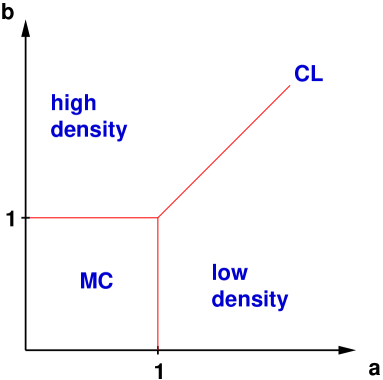
Figure 2: Stationary state phase diagram of the PASEP. The high and low density phases are separated by the coexistence line (CL). The maximum current phase (MC) occurs at small values of the parameters $a$ and $b$ defined in (2.7).

3.2 Dynamical phase diagram

The dynamical phase diagram for the PASEP resulting from our analysis in the regime $q<p=1$ is shown in Figure 3. It exhibits the same subdivision into low and high density phases ($a>1$ and $b>1$), the coexistence line ($a=b>1$) and the maximum current phase ($a,b<1$) found from the analysis of the current in the stationary state [10]. However, the finite-size scaling of the lowest excited state energy of the transition matrix suggests the sub-division of both low and high-density phases into four regions respectively. These regions are characterized by different functional forms of the relaxation rates at asymptotically late times. We will describe the four regions in the low density phase ($a>1$ and $b\leq a$). The results in the high density phase are obtained by exchanging $a\leftrightarrow b$. We note that the results for the relaxation rates presented below are valid in the limit $L\to\infty$ at fixed $q<1$. In particular the limit of symmetric exclusion $q=1$ cannot be obtained by taking the limit $q\to 1$ in the expression presented below.

1. Region I:

   This region is defined by

   $$b\geq q^{2}a\ {\rm for}\ a>q^{-3/2}\ {\rm and}\ b\geq a^{-1/3}\ {\rm for}\ 1<a<q^{-3/2}.$$ (3.1)

   The eigenvalue of the lowest excitation is given by ($q<1$ fixed)

   $$\mathcal{E}_{1} = -(1-q)\left[\frac{1}{1+a}+\frac{1}{1+b}+\frac{2z_{\rm c}}{1-z_{\rm c}}\right]$$ (3.2)

   $$+\frac{(1-q)}{L^{2}}\frac{\pi^{2}}{(z_{\rm c}^{-1}-z_{\rm c})}+{\cal O}(L^{-3}),$$

   where

   $$z_{\rm c}=-\frac{1}{\sqrt{ab}}.$$ (3.3)

2. Coexistence Line:

   The coexistence line is defined by $a=b>1$ and separates the low and high density phases. We find that the leading term in (3.2) vanishes and that the lowest eigenvalue concomitantly scales with the system size as

   $$\mathcal{E}_{1}=\frac{1-q}{L^{2}}\frac{\pi^{2}}{(a^{-1}-a)}+\mathcal{O}(L^{-3}),$$ (3.4)

   The inverse proportionality of the eigenvalue (3.4) to the square of the system size implies a dynamic exponent $z=2$, which in turn suggests that the relaxation at late times is governed by diffusive behaviour.

3. Region II:

   This region is defined by

   $$b\leq a^{-1/3}\ {\rm for}\ 1<a<q^{-3/2}\ .$$ (3.5)

   The eigenvalue of the lowest excitation is now independent of $b$

   $$\mathcal{E}_{1} = -(1-q)\left[\frac{1}{1+a}+\frac{2z_{\rm c}+1}{1-z_{\rm c}}\right]$$ (3.6)

   $$+\frac{1-q}{L^{2}}\frac{4\pi^{2}}{(z_{\rm c}^{-1}-z_{\rm c})}+{\cal O}(L^{-3}),$$

   where

   $$z_{\rm c}=-a^{-1/3}.$$ (3.7)

   We note that the leading terms of $(\ref{E_I})$ and $(\ref{E_II})$ coincide along the boundary $b=a^{-1/3}$ separating the two regimes, but the terms of order $L^{-2}$ exhibit a discontinuity. This suggests a crossing of levels and an associated change in the detailed nature of the corresponding relaxational mode.

4. Region III:

   This region is defined by

   $$q^{1/2}\leq b\leq q^{2}a\ {\rm for}\ a>q^{-3/2}.$$ (3.8)

   Up to terms of order $\mathcal{O}(L^{-3})$, the eigenvalue of the lowest excitation in this region is given by

   $$\mathcal{E}_{1}\approx-(1-q)\left(\frac{1}{1+a}+\frac{1}{1+b}+\frac{qa}{1+qa}+\frac{2z_{\rm c}-1}{1-z_{\rm c}}\right),$$ (3.9)

   where now

   $$z_{\rm c}=-q/b.$$ (3.10)

   We note that the leading terms of $(\ref{E_I})$ and $(\ref{E_III})$ coincide along the boundary $b=q^{2}a$ separating Regions I and III. However, throughout Region III there is no contribution of order ${\cal O}(L^{-2})$ to the transition matrix eigenvalue of the lowest excited state.

5. Region IV:

   This final region is defined by

   $$a>q^{-3/2},\qquad b<q^{1/2}.$$ (3.11)

   The eigenvalue of the lowest excitation in this region is given by

   $$\mathcal{E}_{1} = -(1-q)\left[\frac{1}{1+a}+\frac{qa}{1+qa}+\frac{2z_{\rm c}}{1-z_{\rm c}}\right]$$ (3.12)

   $$+\frac{1-q}{L^{2}}\frac{\pi^{2}}{(z_{\rm c}^{-1}-z_{\rm c})}+{\cal O}(L^{-3}),$$

   where now

   $$z_{\rm c}=-q^{1/2}.$$ (3.13)

   We note that the leading terms of (3.12) and (3.9) match along the boundary between regions IV and III. The same holds for the leading terms of (3.12) and (3.6) along the boundary between regions IV and II. On the other hand, there is a discontinuity in the ${\cal O}(L^{-2})$ contributions in both cases.

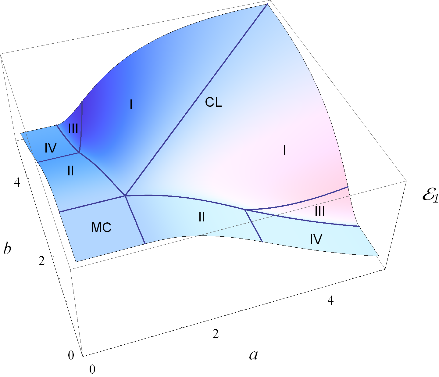
Figure 3: Dynamical phase diagram of the PASEP in the forward bias regime determined by the lowest excitation $\mathcal{E}_{1}$. The horizontal axes are the boundary parameters $a$ and $b$ (2.7) and the vertical axis is the lowest relaxation rate ${\cal E}_{1}$. The latter goes to zero for large systems on the coexistence line (CL) and in the maximum current phase (MC). The curves and lines correspond to various crossovers in the low and high density phase, across which $\mathcal{E}_{1}$ changes non-analytically. See the main text for a detailed explanation.

3.3 Modified domain wall theory

It was shown in [26, 27] that the diffusive relaxation towards the stationary state found on the coexistence line as well as in the low and high density phases can be understood in terms of an effective domain wall theory (DWT). In this approach the excited states driving the relaxational dynamics are modelled as domain walls between low and high density regions. They carry out a random walk with right and left hopping rates given by

$$D_{\pm}=(1-q)\frac{\rho^{\pm}(1-\rho^{\pm})}{\rho^{+}-\rho^{-}}.$$ (3.14)

Here, $\rho^{-}=1/(1+a)$ and $\rho^{+}=b/(1+b)$ are the stationary bulk densities in the low and high-density phases respectively. The domain walls are assumed to be reflected from both boundaries. Interestingly, domain wall theory gives the exact stationary state along the curve $ab=q^{-1}$ in parameter space [45]. It is furthermore possible to construct an entire family of exact domain wall solutions of the master equation [45] . The leading relaxation rate calculated from these exact domain wall solutions agrees with our results (3.2) and (3.4) in Region I and the coexistence line. This suggests that DWT gives a correct description of the relaxational behaviour at late times throughout these regimes.

In contrast, the eigenvalue of the transition matrix determined from DWT does not coincide with our results in Regions II-IV . This means that while the shock profile considered in [45] remains the exact stationary state along the curve $abq=1$, the slowest relaxational mode is no longer given by the particular implementation of DWT proposed in [26, 27]. An obvious question is whether it is possible to reproduce our findings by a suitably modified DWT.

To this end it is useful to consider our results for the eigenvalue of the lowest excited state as a function of $b$ for fixed $a$ and $q$. A particular example ($a=1.5$ and $q=0.6$) is shown in Fig. 4.

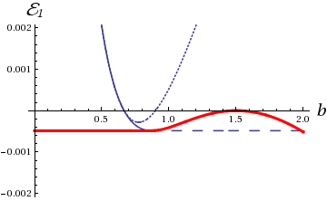
Figure 4: The lowest excitation for $q=0.6$ and $a=1.5$. The functions defined in (3.2), (3.9) (dotted) and (3.6) (dashed) are both displayed for $0<b<2$. The excitation gap is a combination of (3.2) and (3.6), and drawn as the bold curve (red online).

When $b>a$ we are in the high density phase and the system is gapped. The corresponding gap is finite and given by (3.2). Decreasing $b$ we are approaching the coexistence line $b=a$, where the gap vanishes and the relaxation is purely diffusive. Decreasing $b$ further drives us into the low density phase and the gap is again finite. We expect the gap to grow as $b$ decreases. However, at $b_{\rm c}=a^{-1/3}$ ($\approx 0.87$ in the example shown in Fig. 4), the slope of (3.2) as a function of $b$ vanishes and for $b<b_{\rm c}$ (3.2) increases with decreasing $b$. For values of $b$ smaller than the crossover point $b_{\rm c}$, the gap is no longer described by (3.2) but by (3.6), and remains constant.

It is now straightforward to reproduce these results within the framework of an effective DWT. In Region I the DWT prediction [45] for the gap coincides with (3.2)

$$\mathcal{E}_{1}(\rho^{-},\rho^{+})=-D_{+}-D_{-}+2\sqrt{D_{+}D_{-}}\ ,$$ (3.15)

where $D_{\pm}$ are defined above. However, as we cross over into Region II the gap predicted by this DWT no longer agrees with the exact result. We therefore modify the DWT as follows. We postulate that in Region II the density $\rho^{+}$ ceases to depend on $b$ and remains fixed at $\rho^{+}_{\rm eff}=b_{\rm c}/1+b_{\rm c}$. Retaining the expressions (3.14) for the hopping rates of the domain wall one finds that the gap is then given by $\mathcal{E}_{1}(\rho^{-},\rho^{+}_{\rm eff})$. The value of $\rho^{+}_{\rm eff}$ is determined from the requirement that

$$\left.\frac{\partial\mathcal{E}_{1}(\rho^{-},\rho^{+})}{\partial\rho^{+}}\right|_{\rho^{+}=\rho^{+}_{\rm eff}}=0.$$ (3.16)

By construction this modified DWT reproduces the exact result for the relaxation rate.

The modification of the DWT becomes more involved if $a>q^{-3/2}$. In this case there are two crossovers as is shown in Fig. 5 for the particular example $q=0.8$ and $a=3$.

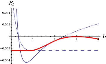
Figure 5: Eigenvalue of the lowest excitation for $q=0.8$ and $a=3$. The functions defined in (3.2), (3.9) (dotted) and (3.12) (dashed) are displayed for $0<b<4$. The excitation gap is a combination of all three, and drawn as the bold curve (red online).

The first crossover separating Regions I and III takes place at $b_{{\rm c},1}=q^{2}a$ ($\approx 1.92$ for the example shown in Fig. 5). For values of $b<b_{{\rm c},1}$ the gap is given by (3.9). In this case the $\mathcal{O}(L^{-2})$ correction to $\mathcal{E}_{1}$ vanishes. A second crossover, now between Regions III and IV, occurs at $b_{{\rm c},2}=q^{1/2}$ ($\approx 0.89$ in the example shown in Fig. 5) where

$$\left.\frac{\partial\mathcal{E}_{1}(\rho^{-},\rho^{+})}{\partial\rho^{+}}\right|_{\rho^{+}=\rho^{+}_{\rm eff}}=0.$$ (3.17)

For values of $b<b_{{\rm c},2}$ the relaxation rate is given by (3.9) and no longer depends on $b$.

It is clearly possible to reproduce the exact relaxation rates by adjusting the densities $\rho^{\pm}$ in the DWT accordingly. Unlike above, in this case we do not have a convincing heuristic argument for the first crossover. The modifications of DWT described here are completely ad hoc, all we can say is that at the boundaries between the various regions, levels cross and the precise nature of the relaxational dynamics changes. It would be very interesting to investigate whether in Regions II-IV the relevant excited states are still domain walls.

4 Analysis of the Bethe ansatz equations

In the following we derive the results summarised in the previous section. To this end we analyse (2.1) and (2.3) in the limit or large lattice lengths $L$. It is convenient to introduce functions

$$g(z) = \ln\left(\frac{z(1-qz)^{2}}{(z-1)^{2}}\right),$$ (4.1)

$$g_{\rm b}(z) = \ln\left(\frac{z(1-q^{2}z^{2})}{1-z^{2}}\right)+\ln\left(\frac{z+a}{1+qaz}\frac{1+c/z}{1+qcz}\right)$$ (4.2)

$${}+\ln\left(\frac{z+b}{1+qbz}\frac{1+d/z}{1+qdz}\right).$$

The central object of our analysis is the “counting function” [39, 40, 41],

$${\rm i}Y_{L}(z)=g(z)+\frac{1}{L}g_{\rm b}(z)+\frac{1}{L}\sum_{l=1}^{L-1}K(z_{l},z),$$ (4.3)

where $K(w,z)$ is given by

$$K(w,z)=-\ln\left(\frac{w-qz}{1-qw/z}\frac{1-q^{2}zw}{1-wz}\right).$$ (4.4)

Using the counting function, the Bethe ansatz equations (2.3) can be cast in logarithmic form as

$$Y_{L}(z_{j})=\frac{2\pi}{L}I_{j}\ ,\qquad j=1,\ldots,L-1.$$ (4.5)

Here $I_{j}$ are integer numbers. Each set of integers $\{I_{j}|\;j=1,\ldots,L-1\}$ in (4.5) specifies a particular (excited) eigenstate of the transition matrix. Based on numerical solutions of (4.5) using standard root finding techniques, we assume that the first excited state always corresponds to the same set of integers

$$I_{j}=-L/2+j\quad{\rm for}\quad j=1,\ldots,L-1.$$ (4.6)

The corresponding roots lie on a simple curve in the complex plane, which approaches a closed contour as $L\rightarrow\infty$. The latter fact is more easily appreciated by considering the locus of reciprocal roots $z_{j}^{-1}$ rather than the locus of roots $z_{j}$. In Fig. 6 we present results for $a=\kappa^{+}_{\alpha,\gamma}=5$, $b=\kappa^{+}_{\beta,\delta}=2$, $c=\kappa^{-}_{\alpha,\gamma}=-0.01$, $d=\kappa^{-}_{\beta,\delta}=-0.023$, $q=0.1$ and $L=150$.

Figure 6: Root distribution and reciprocal root distributions for $a=\kappa^{+}_{\alpha,\gamma}=5$, $b=\kappa^{+}_{\beta,\delta}=2$, $c=\kappa^{-}_{\alpha,\gamma}=-0.01$, $d=\kappa^{-}_{\beta,\delta}=-0.023$, $q=0.1$ and $L=150$

In order to compute the exact large $L$ asymptotics of the spectral gap, we derive an integro-differential equation for the counting function $Y_{L}(z)$ in the limit $L\rightarrow\infty$. As a simple consequence of the residue theorem we can write

$$\frac{1}{L}\sum_{j=1}^{L-1}f(z_{j})=\oint_{C_{1}+C_{2}}\frac{dz}{4\pi{\rm i}}\ f(z)Y_{L}^{\prime}(z)\cot\left(\frac{1}{2}LY_{L}(z)\right),$$ (4.7)

where $C=C_{1}+C_{2}$ is a contour enclosing all the roots $z_{j}$, $C_{1}$ being the “interior” and $C_{2}$ the “exterior” part, see Fig. 7. The contours $C_{1}$ and $C_{2}$ intersect in appropriately chosen points $\xi$ and $\xi^{*}$. It is convenient to fix the end points $\xi$ and $\xi^{*}$ by the requirement

$$Y_{L}(\xi^{*})=-\pi+\frac{\pi}{L},\qquad Y_{L}(\xi)=\pi-\frac{\pi}{L}.$$ (4.8)

Using (4.8) in (4.3) we obtain a nonlinear integro-differential equation for the counting function $Y_{L}(z)$. Our goal is to solve this equation for large lattice lengths $L$ through an expansion in inverse powers of $L$. In order to do so we first rewrite (4.7) by separating the contributions coming from $C_{1}$ and $C_{2}$. When doing this it is useful to note that on the contour of integration we have by definition of the counting function that ${\rm Im}Y_{L}(z)=0$. As a result the imaginary part of $Y_{L}(z)$ is positive on $C_{1}$ and negative on $C_{2}$. Using the fact that integration from $\xi^{*}$ to $\xi$ over the contour formed by the roots is equal to half that over $C_{2}-C_{1}$ we find,

$${\rm i}\,Y_{L}(z) = g(z)+\frac{1}{L}g_{\rm b}(z)+\frac{1}{2\pi}\int_{\xi^{*}}^{\xi}K(w,z)Y^{\prime}_{L}(w){\rm d}w$$ (4.9)

$$+\frac{1}{2\pi}\int_{C_{1}}\frac{K(w,z)Y^{\prime}_{L}(w)}{1-{\rm e}^{-{\rm i}LY_{L}(w)}}\,{\rm d}w+\frac{1}{2\pi}\int_{C_{2}}\frac{K(w,z)Y^{\prime}_{L}(w)}{{\rm e}^{{\rm i}LY_{L}(w)}-1}\,{\rm d}w,$$

where we have chosen the branch cut of $K(w,z)$ to lie along the negative real axis.

Figure 7: Sketch of the contour of integration $C$ in (4.7). The open dots correspond to the roots $z_{j}$ and $\xi$ is chosen close to $z_{L-1}$ and avoiding poles of $\cot(LY_{L}(z)/2)$.

Our strategy is to solve the integro-differential equation (4.9) by iteration. Once we have constructed the desired solution $Y_{L}(z)$ we determine the corresponding eigenvalue of the transition matrix from equation (2.1) by turning the sum over roots into an integral using (4.7)

$$\mathcal{E} = -\mathcal{E}_{0}-\frac{L}{2\pi}\int_{\xi^{*}}^{\xi}\varepsilon(z)Y_{L}^{\prime}(z)\,{\rm d}z$$ (4.10)

$$-\frac{L}{2\pi}\int_{C_{1}}\frac{\varepsilon(z)Y^{\prime}_{L}(z)}{1-{\rm e}^{-{\rm i}LY_{L}(z)}}\,{\rm d}z-\frac{L}{2\pi}\int_{C_{2}}\frac{\varepsilon(z)Y^{\prime}_{L}(z)}{{\rm e}^{{\rm i}LY_{L}(z)}-1}\,{\rm d}z.$$

Here the constant ${\mathcal{E}}_{0}$ was defined previously in (2.8) and the “bare energy” $\varepsilon(z)$ is

$$\varepsilon(z) = \frac{(q-1)^{2}z}{(1-z)(qz-1)}=(1-q)\left(\frac{1}{z-1}-\frac{1}{qz-1}\right).$$ (4.11)

5 Low and High Density Phases

The low density phase for $q<1$ is characterized by $a>1$ and $b<1$, while the high density phase corresponds to $a<1$ and $b>1$. In these phases we find that the locations of the end points $\xi$ and $\xi^{*}$ are such that a straightforward expansion of the correction term in (4.9) in inverse powers of $L$ is possible (see e.g. [42, 43] and B). The result is

$${\rm i}\,Y_{L}(z) = g(z)+\frac{1}{L}g_{\rm b}(z)+\frac{1}{2\pi}\int_{\xi^{*}}^{\xi}K(w,z)Y^{\prime}_{L}(w){\rm d}w$$ (5.1)

$${}+\frac{\pi}{12L^{2}}\left(\frac{K^{\prime}(\xi^{*},z)}{Y^{\prime}_{L}(\xi^{*})}-\frac{K^{\prime}(\xi,z)}{Y^{\prime}_{L}(\xi)}\right)+\mathcal{O}(L^{-4}),$$

where the derivatives of $K$ are with respect to the first argument. We note that here we have implicitly assumed that $Y^{\prime}_{L}(\xi)$ is nonzero and of order ${\cal O}(L^{0})$. The integral from $\xi^{*}$ to $\xi$ is along the contour formed by the roots, see Fig. 7. In order to utilize complex analysis techniques it is useful to extend the integration contour beyond the endpoints, so that it pinches the negative real axis at points $z_{\rm c}^{\pm}=z_{\rm c}\pm{\rm i}0$ ($z_{\rm c}\in{\mathbb{R}}$). This leads to the following expression

$${\rm i}\,Y_{L}(z) = g(z)+\frac{1}{L}g_{\rm b}(z)+\frac{1}{2\pi}\int_{z_{\rm c}^{-}}^{z_{\rm c}^{+}}K(w,z)Y^{\prime}_{L}(w){\rm d}w$$ (5.2)

$${}+\frac{1}{2\pi}\int_{\xi^{*}}^{z_{\rm c}^{-}}K(w,z)Y^{\prime}_{L}(w){\rm d}w+\frac{1}{2\pi}\int_{z_{\rm c}^{+}}^{\xi}K(w,z)Y^{\prime}_{L}(w){\rm d}w$$

$${}+\frac{\pi}{12L^{2}}\left(\frac{K^{\prime}(\xi^{*},z)}{Y^{\prime}_{L}(\xi^{*})}-\frac{K^{\prime}(\xi,z)}{Y^{\prime}_{L}(\xi)}\right)+\mathcal{O}(L^{-4})\ .$$

The key to the solution of (5.2) is that all terms have simple expansions in inverse powers of $L$. In order to find the eigenvalue (4.10) up to order ${\cal O}(L^{-2})$ we need to solve (5.2) to order ${\cal O}(L^{-3})$. Substituting the expansions

$$Y_{L}(z)=\sum_{n=0}^{\infty}L^{-n}y_{n}(z),\qquad\xi=z_{\rm c}+\sum_{n=1}^{\infty}L^{-n}(\delta_{n}+{\rm i}\eta_{n}),$$ (5.3)

back into (5.2) yields a hierarchy of integro-differential equations for the functions $y_{n}(z)$

$$y_{n}(z)=g_{n}(z)+\frac{1}{2\pi{\rm i}}\int_{z_{\rm c}^{-}}^{z_{\rm c}^{+}}K(w,z)y^{\prime}_{n}(w)\,{\rm d}w.$$ (5.4)

The integral is along the closed contour following the locus of the roots, see Fig. 7. The first few driving terms $g_{n}(z)$ are given by

$$\begin{array}[]{r@{\hspace{2pt}}c@{\hspace{3pt}}l}g_{0}(z)\hskip 2.0&=\hfil\hskip 3.0&-{\rm i}g(z),\\ g_{1}(z)\hskip 2.0&=\hfil\hskip 3.0&-{\rm i}g_{\rm b}(z)+\kappa_{1}+\lambda_{1}\tilde{K}(z_{\rm c},z),\\ g_{2}(z)\hskip 2.0&=\hfil\hskip 3.0&\kappa_{2}+\lambda_{2}\tilde{K}(z_{\rm c},z)+\mu_{2}K^{\prime}(z_{\rm c},z),\\ g_{3}(z)\hskip 2.0&=\hfil\hskip 3.0&\kappa_{3}+\lambda_{3}\tilde{K}(z_{\rm c},z)+\mu_{3}K^{\prime}(z_{\rm c},z)+\nu_{3}K^{\prime\prime}(z_{\rm c},z).\end{array}$$ (5.5)

The functions $g$ and $g_{\rm b}$ are defined in (4.1) and (4.2) and

$$\tilde{K}(z_{\rm c},z)=-\ln(-z_{\rm c})+\ln\left(\frac{1-qz_{\rm c}z^{-1}}{1-qzz_{\rm c}^{-1}}\frac{1-zz_{\rm c}}{1-q^{2}zz_{\rm c}}\right).$$ (5.6)

The terms involving the kernel and its derivatives arise from Taylor-expanding the integrands in the integrals from $\xi^{*}$ to $z_{\rm c}^{-}$ and from $z_{\rm c}^{+}$ to $\xi$. Concomitantly the coefficients $\kappa_{n}$, $\lambda_{n}$, $\mu_{n}$ and $\nu_{n}$ are given in terms of $\delta_{n}$, $\eta_{n}$ defined by (5.3), and by derivatives of $y_{n}$ evaluated at $z_{\rm c}$. Explicit expressions are presented in C. We show how to construct a general solution of the set of equations (5.4) for $n\leq 3$ under certain restrictions on the values of the parameter $a$, $b$, $c$ and $d$ in A. Having this solution in hand, we may determine the coefficients $\kappa_{n}$, $\lambda_{n}$, $\mu_{n}$ and $\nu_{n}$ as follows. Substituting the expansions (5.3) into the boundary condition (4.8), which fixes the endpoints $\xi$ and $\xi^{*}$, we obtain a hierarchy of conditions for $y_{n}(z_{\rm c})$, e.g.

$$Y_{L}(\xi) = y_{0}(\xi)+\frac{1}{L}y_{1}(\xi)+\frac{1}{L^{2}}y_{2}(\xi)+\ldots$$ (5.7)

$$= y_{0}(z_{\rm c})+\frac{1}{L}\left[y_{1}(z_{\rm c})+y_{0}^{\prime}(z_{\rm c})(\delta_{1}+i\eta_{1})\right]+\ldots$$

$$= \pi-\frac{\pi}{L}\ .$$

Solving this equation order by order, we find that in all cases considered in the present work

$$\begin{array}[]{r@{\hspace{2pt}}c@{\hspace{3pt}}l}\lambda_{3}\hskip 2.0&=\hfil\hskip 3.0&\mu_{2}=\lambda_{2}=\kappa_{1}=0,\\ \nu_{3}\hskip 2.0&=\hfil\hskip 3.0&\displaystyle z_{\rm c}\mu_{3}=\frac{\lambda_{1}}{2{\rm i}}z_{\rm c}(z_{\rm c}-1)^{2}\kappa_{2}=\frac{\pi^{2}\lambda_{1}(1+\lambda_{1}^{2})}{6}\frac{z_{\rm c}^{2}(1-z_{\rm c})^{2}}{(1+z_{\rm c})^{2}}.\end{array}$$ (5.8)

Here the parameter $\lambda_{1}$ depends on the values of $a$ and $b$. As will be described in detail below, it determines various crossover regimes within the low and high density phase.

Having determined the counting function we may use equation (4.10) to evaluate the corresponding eigenvalue of the transition matrix. Evaluating the necessary integrals in the same way as for the counting function itself we obtain

$${\cal E}=-\mathcal{E}_{0}-\frac{L}{2\pi}\oint_{z_{\rm c}}\varepsilon(z)Y^{\prime}_{L}(z){\rm d}z-{\rm i}\sum_{n\geq 0}e_{n}L^{-n},$$ (5.9)

where the integral is over the closed contour on which the roots lie, $\varepsilon$ is given in (4.11) and

$$e_{0} = \lambda_{1}\varepsilon(z_{\rm c}),$$

$$e_{1} = \lambda_{2}\varepsilon(z_{\rm c})+\mu_{2}\varepsilon^{\prime}(z_{\rm c}),$$ (5.10)

$$e_{2} = \lambda_{3}\varepsilon(z_{\rm c})+\mu_{3}\varepsilon^{\prime}(z_{\rm c})+\nu_{3}\varepsilon^{\prime\prime}(z_{\rm c}).$$

Substituting the expansion for $Y_{L}(z)$ in inverse powers of $L$ into (5.9) we arrive at the following result for the eigenvalue of the transition matrix with the largest non-zero real part

$$\mathcal{E}_{1} = -(1-q)\left(\frac{1}{1+a}+\frac{1}{1+b}+\frac{2z_{\rm c}-2-{\rm i}\lambda_{1}}{1-z_{\rm c}}-\sum_{m}\frac{c_{m}}{1-z_{m}}\right)$$ (5.11)

$${}+\frac{1}{L^{2}}\frac{(1-q)\,{\rm i}\lambda_{1}(1+\lambda_{1}^{2})\pi^{2}}{6(z_{\rm c}^{-1}-z_{\rm c})}+\mathcal{O}(L^{-3}).$$

Here, the sum over $m$ is over all poles of $g^{\prime}_{\rm b}(z)$ other than $0$, $-c$ and $-d$, that lie inside the contour of integration. The constants $c_{m}$ are the corresponding residues. We note that the number and position of such poles depend on the values of the parameters $a$ and $b$. The values of both $\lambda_{1}$ and $z_{\rm c}$ in turn depend on these poles. In particular we find

$$\lambda_{1}=2{\rm i}+{\rm i}\sum_{m}c_{m}\ .$$ (5.12)

The result (5.11) for the smallest relaxation rate is generically a constant of order ${\cal O}(L^{0})$, implying an exponentially fast relaxation to the stationary state at large times. We note that due to the symmetry of the root distribution corresponding to (4.6) under complex conjugation, ${\cal E}_{1}$ is in fact real, and hence there are no oscillations in the slowest relaxation mode.

5.1 Region I: large values of $a$ and $b$

The first regime we consider is obtained loosely speaking by taking $q$ to be small, $a$ and $b$ large and positive, $c$ and $d$ small and negative. More precisely we require

1. $-a$ and $-b$ lie outside the contour of integration in (5.2),

2. $-1/qa$ and $-1/qb$ lie outside the contour,

3. $-c$ and $-d$ lie inside the contour of integration.

We will assume that the last assumption is fulfilled, postponing a detailed discussion to Section 6. Condition (i) amounts to the inequalities $-a<z_{\rm c}$ and $-b<z_{\rm c}$, which translate to

$$b>b_{\rm c,1}=a^{-1/3}\quad(a>1),\qquad\quad a>a_{\rm c,1}=b^{-1/3}\quad(b>1).$$ (5.13)

Condition (ii) implies that $-1/qa<z_{\rm c}$ and $-1/qb<z_{\rm c}$, resulting in

$$b<b_{\rm c,2}=q^{2}a\quad(a>1),\qquad\qquad a<a_{\rm c,2}=q^{2}b\quad(b>1).$$ (5.14)

From the distribution of the reciprocal roots, see Fig. 6, we infer that for these values of the parameters, the roots lie in fact inside the unit circle. We therefore assume, and verify a posteriori, that $z_{\rm c}\neq-1$ and that the points $\pm 1$ lie outside the contour of integration. Combining the above assumption we conclude that the driving term (5.5) for (5.4) with $n=1$ can be represented in the form

$$g_{1}(z) = -{\rm i}\ln z-{\rm i}\ln\left(\frac{z+c}{z}\right)-{\rm i}\ln\left(\frac{z+d}{z}\right)$$ (5.15)

$${}+\lambda_{1}\ln\left(\frac{z-qz_{\rm c}}{z}\right)+g_{1}^{\rm a}(z),$$

where $g_{1}^{\rm a}(z)$ is analytic inside the contour of integration. Under the above assumptions we may now solve the system (5.4) of integro-differential equations and then verify a posteriori that all underlying assumptions in fact hold. Some details of this caculation are presented in A. The result for the counting function is $Y_{L}(z)=y_{0}(z)+\frac{1}{L}y_{1}(z)+\frac{1}{L^{2}}y_{2}(z)+\frac{1}{L^{3}}y_{3}(z)+{\cal O}(L^{-4})$ where

$$y_{0}(z) = -{\rm i}\ln\left[-\frac{z}{z_{\rm c}}\left(\frac{1-z_{\rm c}}{1-z}\right)^{2}\right],$$ (5.16)

$$y_{1}(z) = -{\rm i}\ln\left[-\frac{z}{z_{\rm c}}\frac{1-z_{\rm c}^{2}}{1-z^{2}}\right]+\kappa_{1}-{\rm i}\ln\left(ab\right)-\lambda_{1}\ln(-z_{\rm c})$$ (5.17)

$${}-{\rm i}\ln\left[\frac{(-c/z;q)_{\infty}(-cz;q)_{\infty}(-z/a;q)_{\infty}(-qaz_{\rm c};q)_{\infty}}{(-c/z_{\rm c};q)_{\infty}(-cz_{\rm c};q)_{\infty}(-z_{\rm c}/a;q)_{\infty}(-qaz;q)_{\infty}}\right]$$

$${}-{\rm i}\ln\left[\frac{(-d/z;q)_{\infty}(-dz;q)_{\infty}(-z/b;q)_{\infty}(-qbz_{\rm c};q)_{\infty}}{(-d/z_{\rm c};q)_{\infty}(-dz_{\rm c};q)_{\infty}(-z_{\rm c}/b;q)_{\infty}(-qbz;q)_{\infty}}\right]$$

$${}+\lambda_{1}\ln\left[\frac{(qz_{\rm c}/z;q)_{\infty}(qzz_{\rm c};q)_{\infty}^{2}}{(qz/z_{\rm c};q)_{\infty}(qz_{\rm c}^{2};q)_{\infty}^{2}}\right]+\lambda_{1}\ln\left(\frac{z-z_{\rm c}^{-1}}{z_{\rm c}-z_{\rm c}^{-1}}\right),$$

$$y_{2}(z) = \kappa_{2}-\lambda_{2}\ln(-z_{\rm c})-\frac{\mu_{2}}{z_{\rm c}}$$ (5.18)

$${}+\mu_{2}\left[\psi_{1}(z|q^{-1})-\psi_{1}(z|q)+2\psi_{1}(z^{-1}|q^{-1})\right]$$

$${}+\lambda_{2}\ln\left[\frac{(qz_{\rm c}/z;q)_{\infty}(qzz_{\rm c};q)_{\infty}^{2}}{(qz/z_{\rm c};q)_{\infty}(qz_{\rm c}^{2};q)_{\infty}^{2}}\right]+\lambda_{2}\ln\left(\frac{z-z_{\rm c}^{-1}}{z_{\rm c}-z_{\rm c}^{-1}}\right)$$

$${}+\frac{\mu_{2}}{z_{\rm c}^{2}}\left(\frac{1}{z-z_{\rm c}^{-1}}-\frac{1}{z_{\rm c}-z_{\rm c}^{-1}}\right),$$

$$y_{3}(z) = \kappa_{3}-\lambda_{3}\ln(-z_{\rm c})-\frac{\mu_{3}}{z_{\rm c}}+\frac{\nu_{3}}{z_{\rm c}^{2}}$$ (5.19)

$${}+\mu_{3}\left[\psi_{1}(z|q^{-1})-\psi_{1}(z|q)+2\psi_{1}(z^{-1}|q^{-1})\right]$$

$${}+\nu_{3}\left[\psi_{2}(z|q)-\psi_{2}(z|q^{-1})-2\psi_{2}(z^{-1}|q^{-1})\right]$$

$${}+\lambda_{3}\ln\left[\frac{(qz_{\rm c}/z;q)_{\infty}(qzz_{\rm c};q)_{\infty}^{2}}{(qz/z_{\rm c};q)_{\infty}(qz_{\rm c}^{2};q)_{\infty}^{2}}\right]+\lambda_{3}\ln\left(\frac{z-z_{\rm c}^{-1}}{z_{\rm c}-z_{\rm c}^{-1}}\right)$$

$${}+\left(\frac{\mu_{3}}{z_{\rm c}^{2}}-\frac{\nu_{3}}{z_{\rm c}^{3}}\right)\left(\frac{1}{z-z_{\rm c}^{-1}}-\frac{1}{z_{\rm c}-z_{\rm c}^{-1}}\right)$$

$${}-\frac{\nu_{3}}{z_{\rm c}^{3}}\left(\frac{z}{\left(z-z_{\rm c}^{-1}\right)^{2}}-\frac{z_{\rm c}}{\left(z_{\rm c}-z_{\rm c}^{-1}\right)^{2}}\right).$$

Here $(a;q)_{\infty}$ denotes the q-Pochhammer symbol

$$(a;q)_{\infty}=\prod_{k=0}^{\infty}(1-aq^{k}),$$ (5.20)

and we have defined functions

$$\psi_{k}(z|q)=\sum_{n=0}^{\infty}\frac{1}{(z_{c}-q^{n+1}z)^{k}}-\frac{1}{z_{c}^{k}(1-q^{n+1})^{k}}\ .$$ (5.21)

Imposing the boundary conditions (4.8), (5.7) and using the expressions presented in C for the various constants we obtain

$$\lambda_{1}=2{\rm i},\qquad z_{\rm c}=-\frac{1}{\sqrt{ab}},$$ (5.22)

and

$$\begin{array}[]{r@{\hspace{2pt}}c@{\hspace{3pt}}l}\lambda_{3}\hskip 2.0&=\hfil\hskip 3.0&\mu_{2}=\lambda_{2}=\kappa_{1}=0,\\ \nu_{3}\hskip 2.0&=\hfil\hskip 3.0&\displaystyle z_{\rm c}\mu_{3}=z_{\rm c}(z_{\rm c}-1)^{2}\kappa_{2}=-{\rm i}\pi^{2}\frac{z_{\rm c}^{2}(1-z_{\rm c})^{2}}{(1+z_{\rm c})^{2}}.\end{array}$$ (5.23)

This is in agreement with our previous assertion (5.8). Given our result for the counting function we may then determine the corresponding eigenvalue of the transition matrix from (5.9)

$$\mathcal{E}_{1} = -(1-q)\left(\frac{1}{1+a}+\frac{1}{1+b}+\frac{2z_{\rm c}}{1-z_{\rm c}}\right)$$ (5.24)

$$+\frac{1}{L^{2}}\frac{(1-q)\,\pi^{2}}{(z_{\rm c}^{-1}-z_{\rm c})}+{\cal O}(L^{-3}),$$

which is the result given in (3.2).

5.2 Region II: $-b$ inside the contour

We now consider the case where $-b$ moves inside the contour, but where the pole at $-1/qa$ remains outside, i.e.

$$b<b_{\rm c}=a^{-1/3}\quad(a>1).$$ (5.25)

The case where $a<a_{\rm c}$ is readily obtained from the results below by the interchange $a\leftrightarrow b$. The main difference compared to Region I is that the driving term $g_{1}(z)$ acquires an additional branch point inside the contour of integration. The ${\cal O}(L^{-1})$ contribution $y_{1}(z)$ to the counting function must therefore be determined on the basis of a different analytic structure of the driving term $g_{1}(z)$:

$$g_{1}(z) = -{\rm i}\ln z-{\rm i}\ln\left(\frac{z+c}{z}\right)-{\rm i}\ln\left(\frac{z+d}{z}\right)$$ (5.26)

$${}+\lambda_{1}\ln\left(\frac{z-qz_{\rm c}}{z}\right)-{\rm i}\ln(z+b)+g_{1}^{\rm a}(z),$$

where $g_{1}^{\rm a}(z)$ is analytic inside the contour. The solution of the corresponding integro-differential equation proceeds along the same lines as before, resulting in the expression (1.31) for $y_{1}(z)$. The solutions of the equations for $y_{2}(z)$ and $y_{3}(z)$ remain unchanged. Imposing the boundary conditions (4.8) imposes $\lambda_{1}=3{\rm i}$ and $z_{\rm c}=-a^{-1/3}$, resulting in the eigenvalue (3.6).

5.3 Region III: $-1/qa$ inside the contour

The next case we consider is when $-1/qa$ lies inside and $-b$ outside the integration contour, which occurs in the parameter regime $q^{1/2}<b<q^{2}a$. The driving term $g_{1}(z)$ of the integro-differential equation for $y_{z}(z)$ is expressed as

$$g_{1}(z) = -{\rm i}\ln\left(\frac{z+c}{z}\right)-{\rm i}\ln\left(\frac{z+d}{z}\right)$$ (5.27)

$${}+\lambda_{1}\ln\left(\frac{z-qz_{\rm c}}{z}\right)+{\rm i}\ln\left(\frac{z+1/qa}{z}\right)+g_{1}^{\rm a}(z),$$

where $g_{1}^{\rm a}(z)$ is analytic inside the contour of integration. Proceeding as before we arrive at the result for $y_{1}(z)$ given in (1.36). The results for $y_{2}(z)$ and $y_{3}(z)$ are the same as before and are given in (5.18) and (5.19). Imposing the boundary conditions (4.8) fixes $\lambda_{1}={\rm i}$ and $z_{\rm c}=-q/b$, leading to the eigenvalue given in (3.9).

5.4 Region IV: $-1/qa$ and $-b$ inside the contour

The last case we consider is when both $-1/qa$ and $-b$ lie inside the contour of integration. This occurs when $a>q^{-3/2}$ and $b<q^{1/2}$. We may express $g_{1}(z)$ in the form

$$g_{1}(z) = -{\rm i}\ln\left(\frac{z+c}{z}\right)-{\rm i}\ln\left(\frac{z+d}{z}\right)-{\rm i}\ln(z+b)$$ (5.28)

$${}+\lambda_{1}\ln\left(\frac{z-qz_{\rm c}}{z}\right)+{\rm i}\ln\left(\frac{z+1/qa}{z}\right)+g_{1}^{\rm a}(z),$$

where $g_{1}^{\rm a}(z)$ is again analytic inside the contour and then proceed as in the other cases. Solving the integro-differential equation for $y_{1}(z)$ results in (1.41). The results for $y_{2}(z)$ and $y_{3}(z)$ are again given by (5.18) and (5.19) respectively. Imposing the boundary conditions (4.8) now gives $\lambda_{1}=2{\rm i}$ and $z_{\rm c}=-q^{1/2}$ and leads to the eigenvalue given in (3.12).

6 Dependence on $c$ and $d$

In all calculations described above we have assumed that both $-c$ and $-d$ lie inside the contour of integration. This is the case if

$$-c<z^{*}\quad\textrm{and}\quad-d<z^{*},$$ (6.1)

where $z^{*}$ is the point where the contour crosses the positive real axis, i.e. the solution of the equation $Y_{L}(z^{*})=0$. In leading order this is determined by the solution of

$$-\frac{z^{*}}{z_{\rm c}}\frac{(1-z_{\rm c})^{2}}{(1-z^{*})^{2}}=1.$$ (6.2)

This condition is easily solved for $z^{*}$ as a function of $z_{c}$ and using the explicit expressions for $z_{\rm c}$ in Regions I-IV we obtain corresponding restrictions on the allowed values of $c$ and $d$. For example, in Region I we find

$$-c,-d<z^{*}(a,b)=\frac{1+4\sqrt{ab}+ab-\sqrt{(1+4\sqrt{ab}+ab)^{2}-4ab}}{2\sqrt{ab}}.$$ (6.3)

However, as we will now show, the results in the high and low density phases presented above have a somewhat larger realm of validity than suggested by (6.3). To that end let us consider the situation where $-d$ is still inside the contour of integration, but $-c$ is slightly larger than $z^{*}(a,b)$. Then the root distribution corresponding to the largest eigenvalue has the same set of integers as before

$$Y_{L}(z_{j})=-\pi+\frac{2\pi j}{L},$$ (6.4)

but the root distribution now has an isolated root $\zeta$ lying outside the contour of integration. The position of the isolated root is

$$\zeta=-c+{\cal O}(e^{-\nu L}),$$ (6.5)

where $\nu>0$. In Fig. 8 the root distribution is depicted for a specific case with $c=-0.2$, and it can be seen that $\zeta\approx-c$. The value of $z^{*}(a,b)$ in this case is approximately $0.136$.

Figure 8: Root distributions for $a=\kappa^{+}_{\alpha,\gamma}=5$, $b=\kappa^{+}_{\beta,\delta}=2$, $c=\kappa^{-}_{\alpha,\gamma}=-0.2$, $d=\kappa^{-}_{\beta,\delta}=-0.023$, $q=0.1$ and $L=50$

.

In order to turn the summation over this distribution of roots into an integral, the contour $C_{2}$ of Figure 7 has to be extended to include the isolated root $\zeta$. This is achieved by adding a contour that runs from $z^{*}+{\rm i}0$ to $\zeta+{\rm i}0$ and back from $\zeta-{\rm i}0$ to $z^{*}-{\rm i}0$. Importantly the extra contour does not encircle any other poles or branch points of the counting function. Hence the analysis of this case is exactly the same as before, and the eigenvalue is again given by (5.24)

The situation becomes more complicated when $-c$ is increased further. Now several isolated roots may lie on the positive real axis outside the contour, close to points $-q^{n}c$ for $n\in\mathbb{N}$. Naively the same argument as for the case of a single isolated roots applies, but a detailed analysis of such cases is beyond the scope of this publication.

7 Conclusions

In this work we have analyzed the Bethe ansatz equations of the partially asymmetric exclusion process with open boundaries. We have focussed on the parameter regime corresponding to low and high density phases in the stationary state. We have determined the eigenvalue of the transition matrix with the largest non-zero real part, which characterizes the relaxation towards the stationary state at asymptotically late times. We found that both the low and high density phases are subdivided into several regimes, which are characterized by different relaxational behaviours. In the vicinity of the coexistence line which separates low and high density phases the relaxational behaviour can be understood in terms of diffusion of domain walls. In the other regimes such interpretations are still possible, but are not conclusively supported by the available results. A number of open questions remain. We have not studied the parameter regime corresponding to the maximal current phase at stationarity. Furthermore, our analysis has been restricted to the “forward bias regime”, in which the injection/extraction rates at the boundaries are compatible with the bias present in the bulk. It would be interesting to extend our analysis to the maximum current phase as well as the “reverse bias regime”. Another open issue is the precise physical nature of the relaxational mechanism sufficiently far away from the coexistence line. Is the relaxation still driven by diffusion of some kind of domain walls, or does another mechanism take over? This issue is particularly relevant in Region III, which occupies a large part of the phase diagram when $q\rightarrow 1$. For symmetric diffusion $q=1$ the relaxation is known to be diffusive and the spectral gap scales as $\mathcal{O}(L^{-2})$. Further interesting questions are whether the Bethe ansatz solution of the open XXZ chain can be used to calculate current fluctuations [47] and whether it is possible to determine correlation functions by means of Bethe ansatz [48]. Perhaps recent algebraic insights may offer new tools for further analysis. Such insights include the PASEP being an exceptional representation of the two-boundary Temperley-Lieb algebra [49] through the connection with the open spin chain [31], or the connection with tridiagonal algebras [50, 51].

Appendix A Details on the calculation of the counting function

In this Appendix we describe how to solve the integro-differential equation for the counting function. We start by deriving a simple identity that proves to be very useful in the subsequent analysis. Let $C$ be the contour of integration from $z_{\rm c}^{-}$ to $z_{\rm c}^{+}$ defined by the locus of roots, c.f. Fig.7. Let $D$ denote the interior of $C$ and $f^{\prime}(z)$ be an analytic function in $D$. Then elementary considerations show that

$$\frac{1}{2\pi{\rm i}}\int_{z_{\rm c}^{-}}^{z_{\rm c}^{+}}\ln(w-z)\left(\frac{1}{w-a}+f^{\prime}(w)\right)\,{\rm d}w =$$ (1.3)

$$\hphantom{}\left\{\begin{array}[]{ll}\displaystyle\ln\left(\frac{z_{\rm c}-a}{z-a}\right)+f(z_{\rm c})-f(z)&{\rm if}\ a\not\in D,\ z\in D,\\ \ln(a-z_{\rm c})+f(z_{\rm c})-f(z)&{\rm if}\ a,z\in D.\end{array}\right.$$

Here, for every $w$, we have placed the branch cut of $\ln(w-z)$ along the line from $z$ to $z_{\rm c}$ so that the left hand side is a well defined contour integral. The identity (1.3) is useful for constructing solutions of the integro-differential equations (5.4). In particular, if $y(z)$ is given by

$$y(z)=y^{\rm a}(z)+\sum_{m}A_{m}\ln(z-z_{m}),$$ (1.4)

where ${\rm d}y^{\rm a}(z)/{\rm d}z$ is analytic in $D$, then, for $z$ close to the locus of the roots,

$$\frac{1}{2\pi{\rm i}}\oint_{z_{\rm c}}K(w,z)y^{\prime}(w){\rm d}w=y(qz)-y(z_{\rm c})+\sum_{m}A_{m}K(z_{m},z).$$ (1.5)

Here the kernel $K(w,z)$ is given in (4.4) whose branch cut we take as above. The condition on $z$ is that $1/z$, $1/q^{2}z$ and $z/q$ all lie outside the contour of integration ($z/q$ lies outside the contour as we take $z$ to be very close to the latter).

A.1 Region I: large values of $a$ and $b$

We first consider the case

1. $-c$ and $-d$ are inside $D$,

2. $\pm 1$, $-a$, $-b$, $-1/qa$ and $-1/qb$ are outside $D$.

Loosely speaking this corresponds to small $q$, large positive $a$ and $b$ and small negative $c$ and $d$. We further assume (and verify a posteriori) that $D$ lies inside the unit circle, and hence that the point $1/qc$ and $1/qd$ also lie outside $D$.

We wish to solve the system of integro-differential equations (5.4):

$$y_{n}(z)=g_{n}(z)+\frac{1}{2\pi{\rm i}}\int_{z_{\rm c}^{-}}^{z_{\rm c}^{+}}K(w,z)y^{\prime}_{n}(w)\,{\rm d}w,$$ (1.6)

where the driving terms $g_{n}(z)$ are given in (5.5). We note that the equations are coupled as the driving terms of the equations for larger $n$ depend on the solutions for smaller values of $n$. In the following we construct a solution of (1.6) and verify a posteriori that the above assumptions hold.

A.1.1 Equation for $y_{0}(z)$:

The driving term of the leading equation is given by

$$g_{0}(z)=-{\rm i}g(z)=-{\rm i}\ln z-2{\rm i}\ln\left(\frac{1-qz}{1-z}\right)=-{\rm i}\ln z+g_{0}^{\rm a}(z).$$ (1.7)

Here $g_{0}^{a}(z)$ is analytic in $D$. We assume that $y_{0}(z)$ has the same analytic structure in $D$, i.e.

$$y_{0}(z)=-{\rm i}\ln z+y_{0}^{\rm a}(z),$$ (1.8)

where $y_{0}^{\rm a}(z)$ is analytic. Subsituting this ansatz into the integro-differential equation (1.6) for $n=0$ we obtain from (1.5),

$$y_{0}^{\rm a}(z)=g_{0}^{\rm a}(z)-{\rm i}K(0,z)+y_{0}(qz)-y_{0}(z_{\rm c}).$$ (1.9)

Combining equations (1.8) and (1.9) we obtain a functional equation for $y_{0}^{\rm a}(z)$

$$y_{0}^{\rm a}(z)-y_{0}^{\rm a}(qz)=-2{\rm i}\ln\left(\frac{1-qz}{1-z}\right)+{\rm i}\ln(-z_{\rm c})-y_{0}^{\rm a}(z_{\rm c}).$$ (1.10)

The constant $y_{0}^{\rm a}(z_{\rm c})$ is readily determined by setting $z=0$. The resulting functional equation is then readily solved, giving

$$y_{0}^{\rm a}(z)=2{\rm i}\ln(1-z)-{\rm i}\ln\left(-\frac{(1-z_{\rm c})^{2}}{z_{\rm c}}\right).$$ (1.11)

The zeroeth order term in the expansion of the counting function is then found to be

$$y_{0}(z)=-{\rm i}\ln\left[-\frac{z}{z_{\rm c}}\left(\frac{1-z_{\rm c}}{1-z}\right)^{2}\right].$$ (1.12)

A.1.2 Equation for $y_{1}(z)$:

With the assumptions on $q,a,b,c$ and $d$ stated above the driving term (5.5) of the integro-differential equation (1.6) for $n=1$ can be cast in the form

$$g_{1}(z) = -{\rm i}\ln z-{\rm i}\ln\left(\frac{z+c}{z}\right)-{\rm i}\ln\left(\frac{z+d}{z}\right)$$ (1.13)

$${}+\lambda_{1}\ln\left(\frac{z-qz_{\rm c}}{z}\right)+g_{1}^{\rm a}(z),$$

where $g_{1}^{\rm a}(z)$ is analytic in $D$. The singularities of $y_{1}(z)$ inside the domain $D$ can be inferred by trying to solve the integro-differential equation by iteration. It is then quickly seen that a branch point in $y_{1}(z)$ at $z=-c$ produces a branch point at $z=-qc$, which in turn leads to a branch point at $z=-q^{2}c$ etc. This suggests the following ansatz for $y_{1}(z)$

$$y_{1}(z) = -{\rm i}\ln\left[(-c/z;q)_{\infty}(-d/z;q)_{\infty}\right]+\lambda_{1}\ln(qz_{\rm c}/z;q)_{\infty}$$ (1.14)

$${}-{\rm i}\ln z+y_{1}^{\rm a}(z),$$

where $y_{1}^{\rm a}(z)$ is analytic inside $D$, and the q-Pochhammer symbol $(a;q)_{\infty}$ was defined in (5.20). Substituting (1.14) into (1.6) we find

$$y_{1}^{\rm a}(z) = {\rm i}\ln\left[(-c/qz;q)_{\infty}(-d/qz;q)_{\infty}\right]-\lambda_{1}\ln(z_{\rm c}/z;q)_{\infty}$$ (1.15)

$${}-{\rm i}\ln\left[(1+cz)(1+qcz)(1+dz)(1+qdz)\right]$$

$${}+\lambda_{1}\ln\left[(1-qz_{\rm c}z)(1-q^{2}z_{\rm c}z)\right]+g_{1}^{\rm a}(z)-y_{1}(z_{\rm c})$$

$${}+{\rm i}\ln(-qz)+y_{1}(qz).$$

This leads to the following functional equation for $y_{1}^{\rm a}(z)$

$$y_{1}^{\rm a}(z) = -{\rm i}\ln\left[(1+cz)(1+qcz)(1+dz)(1+qdz)\right]$$ (1.16)

$${}+\lambda_{1}\ln\left[(1-qz_{\rm c}z)(1-q^{2}z_{\rm c}z)\right]$$

$${}+g_{1}^{\rm a}(z)-y_{1}(z_{\rm c})\pm\pi+y_{1}^{\rm a}(qz).$$

The value of $y_{1}(z_{\rm c})$ is easily determined by evaluating (1.16) at $z=0$

$$y_{1}(z_{\rm c})=\pm\pi+g_{1}^{\rm a}(0).$$ (1.17)

Using the fact that for two analytic functions $u$ and $v$, the equation

$$u(z)-u(qz)=v(z),$$ (1.18)

is solved by $u(z)=\sum_{k=0}^{\infty}v(q^{k}z)$, it is now a straightforward matter to solve the functional equation (1.16), leading to the result given in equation (5.17).

A.1.3 Equation for $y_{2}(z)$:

The driving term (5.5) of the integro-differential equation (5.4) for $n=2$ can be represented in the form

$$g_{2}(z)=\lambda_{2}\ln\left(\frac{z-qz_{\rm c}}{z}\right)-\mu_{2}\frac{q}{z-qz_{\rm c}}+g_{2}^{\rm a}(z),$$ (1.19)

where $g_{2}^{\rm a}(z)$ is analytic in $D$. As in the case $n=1$ the singularities of $y_{2}(z)$ inside $D$ can be determined by attempting to solve the equation by iteration. This results in the ansatz

$$y_{2}(z) = \lambda_{2}\ln(qz_{\rm c}/z;q)_{\infty}-\mu_{2}\sum_{n=0}^{\infty}\frac{q^{n+1}}{z-q^{n+1}z_{\rm c}}+y_{2}^{\rm a}(z),$$ (1.20)

where $y_{2}^{\rm a}(z)$ is analytic inside $D$. Substituting (1.20) into (1.6) we obtain a functional equation for $y_{2}^{\rm a}(z)$

$$y_{2}^{\rm a}(z)-y_{2}^{\rm a}(qz) = \kappa_{2}-\lambda_{2}\ln(-z_{c})+\lambda_{2}\ln\left[\frac{(1-z_{\rm c}z)(1-qz_{\rm c}z)}{1-qz/z_{\rm c}}\right]$$ (1.21)

$$- \mu_{2}\left[\frac{qz}{1-qz_{\rm c}z}+\frac{z}{1-z_{\rm c}z}-\frac{1}{qz-z_{\rm c}}\right]-y_{2}(z_{c}).$$

Evaluating (1.21) at $z=0$ fixes the constant to be

$$y_{2}(z_{\rm c})=\kappa_{2}-\lambda_{2}\ln(-z_{\rm c})-\frac{\mu_{2}}{z_{\rm c}}.$$ (1.22)

The functional equation (1.21) is then solved by elementary means, resulting in the expression for $y_{2}(z)$ given in equation (5.18).

A.1.4 Equation for $y_{3}(z)$:

The driving term (5.5) of the integro-differential equation (5.4) for $n=3$ can be represented in the form

$$g_{3}(z)=\lambda_{3}\ln\left(\frac{z-qz_{\rm c}}{z}\right)-\mu_{3}\frac{q}{z-qz_{\rm c}}-\nu_{3}\frac{q^{2}}{(z-qz_{\rm c})^{2}}+g_{3}^{\rm a}(z),$$ (1.23)

where $g_{3}^{\rm a}(z)$ is analytic in $D$. Determining the singularities of $y_{3}(z)$ inside $D$ by iterating the integro-differential equation now results in the ansatz

$$y_{3}(z) = \lambda_{3}\ln(qz_{\rm c}/z;q)_{\infty}-\mu_{3}\sum_{n=0}^{\infty}\frac{q^{n+1}}{z-q^{n+1}z_{\rm c}}$$ (1.24)

$${}-\nu_{3}\sum_{n=0}^{\infty}\frac{q^{2n+2}}{(z-q^{n+1}z_{\rm c})^{2}}+y_{3}^{\rm a}(z),$$

where $y_{3}^{\rm a}(z)$ is analytic inside $D$. Substituting (1.24) into (1.6) for $n=3$ gives a functional equation for $y_{3}^{\rm a}(z)$

$$y_{3}^{\rm a}(z)-y_{3}^{\rm a}(qz) = \kappa_{3}-\lambda_{3}\ln(-z_{c})-y_{3}(z_{c})$$ (1.25)

$$+ \lambda_{3}\ln\left[\frac{(1-z_{\rm c}z)(1-qz_{\rm c}z)}{1-qz/z_{\rm c}}\right]$$

$$- \mu_{3}\left[\frac{qz}{1-qz_{\rm c}z}+\frac{z}{1-z_{\rm c}z}-\frac{1}{qz-z_{\rm c}}\right]$$

$$- \nu_{3}\left[\frac{q^{2}z^{2}}{(1-qz_{\rm c}z)^{2}}+\frac{z^{2}}{(1-z_{\rm c}z)^{2}}-\frac{1}{(qz-z_{\rm c})^{2}}\right].$$

Evaluating (1.25) at $z=0$ again fixed the constant

$$y_{3}(z_{\rm c})=\kappa_{3}-\lambda_{3}\ln(-z_{\rm c})-\frac{\mu_{3}}{z_{\rm c}}+\frac{\nu_{3}}{z_{\rm c}^{2}}.$$ (1.26)

Solving the functional equation (1.25) then results in the expression for $y_{3}(z)$ given in equation (5.19).

A.2 Region II: $-b$ inside the contour of integration

The determination of $y_{n}(z)$ for $n\geq 2$ is exactly the same as in the previous section and in particular the expressions for $y_{2}(z)$ and $y_{3}(z)$ are unchanged and given by (5.18) and (5.19).

A.2.1 Equation for $y_{1}(z)$:

With $-b$ lying inside $D$ the driving term $g_{1}(z)$ may be expressed as

$$g_{1}(z) = -2{\rm i}\ln z-{\rm i}\ln\left(\frac{z+c}{z}\right)-{\rm i}\ln\left(\frac{z+d}{z}\right)$$ (1.27)

$${}+\lambda_{1}\ln\left(\frac{z-qz_{\rm c}}{z}\right)-{\rm i}\ln\left(\frac{z+b}{z}\right)+g_{1,{\rm II}}^{\rm a}(z),$$

where $g_{1,{\rm II}}^{\rm a}(z)$ is analytic in $D$. Proceeding as before, we arrive at the following ansatz for $y_{1}(z)$

$$y_{1}(z) = -{\rm i}\ln\left[(-c/z;q)_{\infty}(-d/z;q)_{\infty}\right]+\lambda_{1}\ln(qz_{\rm c}/z;q)_{\infty}$$ (1.28)

$${}-{\rm i}\ln(-b/z;q)_{\infty}-2{\rm i}\ln z+y_{1}^{\rm a}(z),$$

where $y_{1}^{\rm a}(z)$ is analytic in $D$. Substituting (1.28) into (1.6) we obtain the functional equation

$$y_{1}^{\rm a}(z) = -{\rm i}\ln\left[(1+cz)(1+qcz)(1+dz)(1+qdz)\right]$$ (1.29)

$${}+\lambda_{1}\ln\left[(1-qz_{\rm c}z)(1-q^{2}z_{\rm c}z)\right]-y_{1}(z_{\rm c})\pm 2\pi$$

$${}-{\rm i}\ln\left[(1+bz)(1+qbz)\right]+g_{1,{\rm II}}^{\rm a}(z)+y_{1}^{\rm a}(qz).$$

Evaluating (1.29) at $z=0$ again fixes the constant

$$y_{1}(z_{\rm c})=\pm 2\pi+g_{1,{\rm II}}^{\rm a}(0),$$ (1.30)

and solving (1.29) then results in the following expression for $y_{1}(z)$

$$y_{1}(z) = -2{\rm i}\ln\left[-\frac{z}{z_{\rm c}}\right]-{\rm i}\ln\left[\frac{1-z_{\rm c}^{2}}{1-z^{2}}\right]+\kappa_{1}-{\rm i}\ln\left(a\right)-\lambda_{1}\ln(-z_{\rm c})$$ (1.31)

$${}-{\rm i}\ln\left[\frac{(-c/z;q)_{\infty}(-cz;q)_{\infty}(-z/a;q)_{\infty}(-qaz_{\rm c};q)_{\infty}}{(-c/z_{\rm c};q)_{\infty}(-cz_{\rm c};q)_{\infty}(-z_{\rm c}/a;q)_{\infty}(-qaz;q)_{\infty}}\right]$$

$${}-{\rm i}\ln\left[\frac{(-d/z;q)_{\infty}(-dz;q)_{\infty}(-b/z;q)_{\infty}(-bz;q)_{\infty}}{(-d/z_{\rm c};q)_{\infty}(-dz_{\rm c};q)_{\infty}(-b/z_{\rm c};q)_{\infty}(-bz_{\rm c};q)_{\infty}}\right]$$

$${}+\lambda_{1}\ln\left[\frac{(qz_{\rm c}/z;q)_{\infty}(qzz_{\rm c};q)_{\infty}^{2}}{(qz/z_{\rm c};q)_{\infty}(qz_{\rm c}^{2};q)_{\infty}^{2}}\right]+\lambda_{1}\ln\left(\frac{z-z_{\rm c}^{-1}}{z_{\rm c}-z_{\rm c}^{-1}}\right).$$

A.3 $-1/qa$ inside the contour of integration

The determination of $y_{n}(z)$ for $n\geq 2$ is exactly the same as before and in particular the expressions for $y_{2}(z)$ and $y_{3}(z)$ are unchanged and given by (5.18) and (5.19).

A.3.1 Equation for $y_{1}(z)$:

In this parameter regime $g_{1}(z)$ is expressed as

$$g_{1}(z) = -{\rm i}\ln\left(\frac{z+c}{z}\right)-{\rm i}\ln\left(\frac{z+d}{z}\right)$$ (1.32)

$${}+\lambda_{1}\ln\left(\frac{z-qz_{\rm c}}{z}\right)+{\rm i}\ln\left(\frac{z+1/qa}{z}\right)+g_{1,{\rm III}}^{\rm a}(z),$$

where $g_{1,{\rm III}}^{\rm a}(z)$ is analytic inside $D$. The appropriate ansatz for $y_{1}(z)$ takes the form

$$y_{1}(z) = -{\rm i}\ln\left[(-c/z;q)_{\infty}(-d/z;q)_{\infty}\right]+\lambda_{1}\ln(qz_{\rm c}/z;q)_{\infty}$$ (1.33)

$${}+{\rm i}\ln(-1/qaz;q)_{\infty}+y_{1}^{\rm a}(z),$$

where $y_{1}^{\rm a}(z)$ is analytic inside $D$. Substituting (1.33) into (1.6) we arrive at the functional equation

$$y_{1}^{\rm a}(z) = -{\rm i}\ln\left[(1+cz)(1+qcz)(1+dz)(1+qdz)\right]$$ (1.34)

$${}+\lambda_{1}\ln\left[(1-qz_{\rm c}z)(1-q^{2}z_{\rm c}z)\right]-y_{1}(z_{\rm c})$$

$${}+{\rm i}\ln\left[(1+z/qa)(1+z/a)\right]+g_{1,{\rm III}}^{\rm a}(z)+y_{1}^{\rm a}(qz).$$

Evaluating (1.34) at $z=0$ gives

$$y_{1}(z_{\rm c})=g_{1,{\rm III}}^{\rm a}(0),$$ (1.35)

and we finally arrive at the following expression for $y_{1}(z)$

$$y_{1}(z) = -{\rm i}\ln\left[\frac{1-z_{\rm c}^{2}}{1-z^{2}}\right]+\kappa_{1}-{\rm i}\ln\left(b/q\right)-\lambda_{1}\ln(-z_{\rm c})$$ (1.36)

$${}-{\rm i}\ln\left[\frac{(-c/z;q)_{\infty}(-cz;q)_{\infty}(-1/qaz_{\rm c};q)_{\infty}(-z_{c}/qa;q)_{\infty}}{(-c/z_{\rm c};q)_{\infty}(-cz_{\rm c};q)_{\infty}(-1/qaz;q)_{\infty}(-z/qa;q)_{\infty}}\right]$$

$${}-{\rm i}\ln\left[\frac{(-d/z;q)_{\infty}(-dz;q)_{\infty}(-z/b;q)_{\infty}(-qbz_{\rm c};q)_{\infty}}{(-d/z_{\rm c};q)_{\infty}(-dz_{\rm c};q)_{\infty}(-z_{\rm c}/b;q)_{\infty}(-qbz;q)_{\infty}}\right]$$

$${}+\lambda_{1}\ln\left[\frac{(qz_{\rm c}/z;q)_{\infty}(qzz_{\rm c};q)_{\infty}^{2}}{(qz/z_{\rm c};q)_{\infty}(qz_{\rm c}^{2};q)_{\infty}^{2}}\right]+\lambda_{1}\ln\left(\frac{z-z_{\rm c}^{-1}}{z_{\rm c}-z_{\rm c}^{-1}}\right).$$

A.4 $-b$ and $-1/qa$ inside the contour of integration

The determination of $y_{n}(z)$ for $n\geq 2$ is exactly the same as before and in particular the expressions for $y_{2}(z)$ and $y_{3}(z)$ are unchanged and given by (5.18) and (5.19).

A.4.1 Equation for $y_{1}(z)$:

Now the driving term is expressed as

$$g_{1}(z) = -{\rm i}\ln z-{\rm i}\ln\left(\frac{z+c}{z}\right)-{\rm i}\ln\left(\frac{z+d}{z}\right)-{\rm i}\ln\left(\frac{z+b}{z}\right)$$ (1.37)

$${}+\lambda_{1}\ln\left(\frac{z-qz_{\rm c}}{z}\right)+{\rm i}\ln\left(\frac{z+1/qa}{z}\right)+g_{1,{\rm IV}}^{\rm a}(z),$$

where $g_{1,{\rm IV}}^{\rm a}(z)$ is analytic in $D$. Our ansatz for $y_{1}(z)$ then takes the form

$$y_{1}(z) = -{\rm i}\ln z-{\rm i}\ln\left[(-c/z;q)_{\infty}(-d/z;q)_{\infty}\right]+\lambda_{1}\ln(qz_{\rm c}/z;q)_{\infty}$$ (1.38)

$${}-{\rm i}\ln(-b/z;q)_{\infty}+{\rm i}\ln(-1/qaz;q)_{\infty}+y_{1}^{\rm a}(z),$$

where $y_{1}^{\rm a}(z)$ is analytic. Substituting (1.38) into (1.6) we obtain the functional equation

$$y_{1}^{\rm a}(z) = -{\rm i}\ln\left[(1+cz)(1+qcz)(1+dz)(1+qdz)\right]$$ (1.39)

$${}+\lambda_{1}\ln\left[(1-qz_{\rm c}z)(1-q^{2}z_{\rm c}z)\right]-y_{1}(z_{\rm c})\pm\pi$$

$${}+{\rm i}\ln\left[(1+z/qa)(1+z/a)\right]-{\rm i}\ln\left[(1+bz)(1+qbz)\right]$$

$${}+g_{1,{\rm IV}}^{\rm a}(z)+y_{1}^{\rm a}(qz).$$

Fixing the constant as before gives

$$y_{1}(z_{\rm c})=\pm\pi+g_{1,{\rm IV}}^{\rm a}(0),$$ (1.40)

resulting in

$$y_{1}(z) = -{\rm i}\ln\left[-\frac{z}{z_{\rm c}}\right]-{\rm i}\ln\left[\frac{1-z_{\rm c}^{2}}{1-z^{2}}\right]+\kappa_{1}-{\rm i}\ln\left(q\right)-\lambda_{1}\ln(-z_{\rm c})$$ (1.41)

$${}-{\rm i}\ln\left[\frac{(-c/z;q)_{\infty}(-cz;q)_{\infty}(-1/qaz_{\rm c};q)_{\infty}(-z_{\rm c}/qa;q)_{\infty}}{(-c/z_{\rm c};q)_{\infty}(-cz_{\rm c};q)_{\infty}(-1/qaz;q)_{\infty}(-z/qa;q)_{\infty}}\right]$$

$${}-{\rm i}\ln\left[\frac{(-d/z;q)_{\infty}(-dz;q)_{\infty}(-b/z;q)_{\infty}(-bz;q)_{\infty}}{(-d/z_{\rm c};q)_{\infty}(-dz_{\rm c};q)_{\infty}(-b/z_{\rm c};q)_{\infty}(-bz_{\rm c};q)_{\infty}}\right]$$

$${}+\lambda_{1}\ln\left[\frac{(qz_{\rm c}/z;q)_{\infty}(qzz_{\rm c};q)_{\infty}^{2}}{(qz/z_{\rm c};q)_{\infty}(qz_{\rm c}^{2};q)_{\infty}^{2}}\right]\lambda_{1}\ln\left(\frac{z-z_{\rm c}^{-1}}{z_{\rm c}-z_{\rm c}^{-1}}\right).$$

Appendix B Analysis of the Abel-Plana Formula

In this appendix we sketch how to extract the finite-size correction terms from the integral expression

$${\rm i}\,Y_{L}(z) = g(z)+\frac{1}{L}g_{\rm b}(z)+\frac{1}{2\pi}\int_{\xi^{*}}^{\xi}K(w,z)Y^{\prime}_{L}(w)\ {\rm d}w$$ (2.1)

$$+\frac{1}{2\pi}\int_{C_{1}}\frac{K(w,z)Y^{\prime}_{L}(w)}{1-{\rm e}^{-{\rm i}LY_{L}(w)}}\ {\rm d}w+\frac{1}{2\pi}\int_{C_{2}}\frac{K(w,z)Y^{\prime}_{L}(w)}{{\rm e}^{{\rm i}LY_{L}(w)}-1}\ {\rm d}w.$$

The main contributions to the correction terms in (2.1) comes from the vicinities of the endpoints $\xi$, $\xi^{*}$. Along the contour $C_{1}$ the imaginary part of the counting function is positive, ${\rm Im}(Y_{L}(w))>0$, whereas along the contour $C_{2}$ it is negative, ${\rm Im}(Y_{L}(w))<0$. As a result the integrands decay exponentially with respect to the distance from the endpoints. In the vicinity of $\xi$, we therefore expand

$$Y_{L}(w)=Y_{L}(\xi)+Y_{L}^{\prime}(\xi)(w-\xi)+\ldots\ .$$ (2.2)

Assuming that $Y_{L}^{\prime}(\xi)$ is ${\cal O}(1)$ (an assumption that will be checked self-consistently), we find that the leading contribution for large $L$ is given by

$$\frac{1}{2\pi}\int_{C_{1}}\frac{K(w,z)Y^{\prime}_{L}(w)}{1-{\rm e}^{-{\rm i}LY_{L}(w)}}\ {\rm d}w \sim \frac{Y_{L}^{\prime}(\xi)}{2\pi}\int_{\xi}^{0}\frac{K(w,z)}{1+{\rm e}^{-{\rm i}LY_{L}^{\prime}(\xi)(w-\xi)}}\ {\rm d}w\ ,$$ (2.3)

$$\mbox{}-(\xi\rightarrow\xi^{*}).$$

Here we have used the boundary conditions (4.8). Carrying out the analogous analysis for the integral along the contour $C_{2}$, we arrive at the following expression for the leading contribution of the last two terms in (2.1)

$${\cal A} = \frac{1}{2\pi}\int_{C_{1}}\frac{K(w,z)Y^{\prime}_{L}(w)}{1-{\rm e}^{-{\rm i}LY_{L}(w)}}\ {\rm d}w+\frac{1}{2\pi}\int_{C_{2}}\frac{K(w,z)Y^{\prime}_{L}(w)}{{\rm e}^{{\rm i}LY_{L}(w)}-1}\ {\rm d}w$$ (2.4)

$$= \frac{{\rm i}}{2\pi L}\int_{0}^{\infty}\frac{1}{1+e^{x}}\left[K\Bigl{(}\xi+\frac{{\rm i}\,x}{LY_{L}^{\prime}(\xi)},z\Bigr{)}-K\Bigl{(}\xi-\frac{{\rm i}\,x}{LY_{L}^{\prime}(\xi)},z\Bigr{)}\right]{\rm d}x$$

$$\mbox{}-(\xi\rightarrow\xi^{*}).$$

If the endpoints $\xi,\xi^{*}$ are such that we can Taylor-expand the kernels appearing in (2.4), we can simplify the expression further with the result

$${\cal A} \approx -\frac{K^{\prime}(\xi,z)}{\pi L^{2}Y_{L}^{\prime}(\xi)}\int_{0}^{\infty}\frac{x}{1+e^{x}}\ {\rm d}x\ -\ (\xi\rightarrow\xi^{*})$$ (2.5)

$$= -\frac{\pi}{12L^{2}}\frac{K^{\prime}(\xi,z)}{Y_{L}^{\prime}(\xi)}\ -\ (\xi\rightarrow\xi^{*}).$$

This is the leading Euler-MacLaurin correction term that occurs in the low and high density phases, see (5.2). The key in the above derivation was the ability to expand

$$K\Bigl{(}\xi+\frac{{\rm i}\,x}{LY_{L}^{\prime}(\xi)},z\Bigr{)} - K\Bigl{(}\xi-\frac{{\rm i}\,x}{LY_{L}^{\prime}(\xi)},z\Bigr{)}$$ (2.6)

$$\sim\ln\left[\frac{LY_{L}^{\prime}(\xi)\bigl{(}z^{-1}-\xi\bigr{)}+{\rm i}\,x}{LY_{L}^{\prime}(\xi)\bigl{(}z^{-1}-\xi\bigr{)}-{\rm i}\,x}\right]$$

in a power series in $x$. This is unproblematic as long as $LY_{L}^{\prime}(\xi)\bigl{(}z^{-1}-\xi\bigr{)}$ is large, which turns out to be the case in the low and high density phases as well as on the coexistence line.

Appendix C Expansion coefficients

In this appendix we list the coefficients arising in the expansion (5.4), (5.5) of the integral equation for the counting function $Y_{L}(z)$. In the following list we abbreviate $y^{\prime}_{n}(z_{\rm c})$ by $y^{\prime}_{n}$. We note that by definition $\delta_{n}$ and $\eta_{n}$ are real quantities.

$$\kappa_{1} = -y_{0}^{\prime}\delta_{1},$$ (3.1)

$$\lambda_{1} = y_{0}^{\prime}\frac{\eta_{1}}{\pi},$$ (3.2)

$$\kappa_{2} = -y_{0}^{\prime}\delta_{2}-y_{1}^{\prime}\delta_{1}-\frac{1}{2}y_{0}^{\prime\prime}(\delta_{1}^{2}-\eta_{1}^{2}),$$ (3.3)

$$\lambda_{2} = \frac{1}{\pi}\left(y^{\prime}_{0}\eta_{2}+y^{\prime}_{1}\eta_{1}+y_{0}^{\prime\prime}\delta_{1}\eta_{1}\right),$$ (3.4)

$$\mu_{2} = y^{\prime}_{0}\frac{\delta_{1}\eta_{1}}{\pi},$$ (3.5)

$$\kappa_{3} = -y_{0}^{\prime}\delta_{3}-y_{1}^{\prime}\delta_{2}-y_{2}^{\prime}\delta_{1}-y_{0}^{\prime\prime}(\delta_{1}\delta_{2}-\eta_{1}\eta_{2})-\frac{1}{2}y_{1}^{\prime\prime}(\delta_{1}^{2}-\eta_{1}^{2})$$ (3.6)

$${}-\frac{1}{6}y_{0}^{\prime\prime\prime}\delta_{1}(\delta_{1}^{2}-3\eta_{1}^{2}),$$

$$\lambda_{3} = \frac{1}{\pi}\left(y_{0}^{\prime}\eta_{3}+y_{1}^{\prime}\eta_{2}+y_{2}^{\prime}\eta_{1}+y_{0}^{\prime\prime}(\delta_{1}\eta_{2}+\delta_{2}\eta_{1})+\delta_{1}\eta_{1}y_{1}^{\prime\prime}\right.$$ (3.7)

$$\left.{}+\frac{1}{6}y_{0}^{\prime\prime\prime}\eta_{1}(3\delta_{1}^{2}-\eta_{1}^{2})\right),$$

$$\mu_{3} = \frac{1}{\pi}\left[y_{0}^{\prime}(\delta_{1}\eta_{2}+\delta_{2}\eta_{1})+y_{1}^{\prime}\delta_{1}\eta_{1}+y_{0}^{\prime\prime}\eta_{1}(\delta_{1}^{2}-\frac{\eta_{1}^{2}}{3})+\frac{\pi^{2}y_{0}^{\prime\prime}}{6y_{0}^{\prime 2}}\eta_{1}\right],$$ (3.8)

$$\nu_{3} = \frac{1}{6\pi}\left(y_{0}^{\prime}\eta_{1}(3\delta_{1}^{2}-\eta_{1}^{2})-\pi^{2}\frac{\eta_{1}}{y^{\prime}_{0}}\right).$$ (3.9)

References

References

- [1] F. Spitzer, Adv. Math. 5, 246 (1970).
- [2] T. Liggett, Interacting Particle Systems, Springer, New York 1985.
- [3] B. Derrida, Phys. Rep. 301, 65 (1998);
- [4] G.M. Schütz, Phase Transitions and Critical Phenomena 19 (Academic Press, London, 2000).
- [5] O. Golinelli and K. Mallick, J. Phys. A39, 12679 (2006).
- [6] R.A. Blythe and M.R. Evans, J. Phys. A40, R333 (2007).
- [7] B. Schmittmann and R.K.P. Zia, Statistical Mechanics of Driven Diffusive Systems, in Phase Transitions and Critical Phenomena Vol 17, eds C. Domb and J.L. Lebowitz, Academic Press, London 1995.
- [8] B. Derrida, M. Evans, V. Hakim and V. Pasquier, J. Phys. A26, 1493 (1993).
- [9] G. Schütz and E. Domany, J. Stat. Phys. 72, 277 (1993).
- [10] S. Sandow, Phys. Rev. E50, 2660 (1994).
- [11] F.H.L. Essler and V. Rittenberg, J. Phys. A29, 3375 (1996).
- [12] T. Sasamoto, J. Phys. A32, 7109 (1999), J. Phys. Soc. Jpn 69, 1055 (2000).
- [13] R.A. Blythe, M.R. Evans, F. Colaiori and F.H.L. Essler, J. Phys. A33, 2313 (2000).
- [14] D. Dhar, Phase Transitions 9, 51 (1987).
- [15] L.-H. Gwa and H. Spohn, Phys. Rev. Lett. 68, 725 (1992); Phys. Rev. A 46, 844 (1992).
- [16] D. Kim, Phys. Rev. E 52, 3512 (1995).
- [17] M. Prähofer and H. Spohn, in In and out of equilibrium, ed. V. Sidoravicius, Progress in Probability 51, 185 (Birkhauser Boston, 2002).
- [18] M. Prähofer and H. Spohn, J. Stat. Phys. 108, 1071 (2002).
- [19] P.L. Ferrari and H. Spohn, Comm. Math. Phys. 265, 1 (2006).
- [20] T. Sasamoto, J. Stat. Mech., P07007 (2007).
- [21] T. Imamura and T. Sasamoto, J. Stat. Phys. 128, 799 (2007).
- [22] A. Borodin, P.L. Ferrari, M. Prähofer, T. Sasamoto, J. Stat. Phys. 129, 1055 (2007).
- [23] Z. Nagy, C. Appert and L. Santen, J. Stat. Phys. 109, 623 (2002).
- [24] S. Takesue, T. Mitsudo and H. Hayakawa, Phys. Rev. E 68, 015103 (2003).
- [25] P. Pierobon, A. Parmeggiani, F. von Oppen and E. Frey, Phys. Rev. E72, 036123 (2005).
- [26] A.B. Kolomeisky, G.M. Schütz, E.B. Kolomeisky and J.P. Straley, J. Phys. A31, 6911 (1998).
- [27] M. Dudzinski and G.M. Schütz, J.Phys. A 33, 8351 (2000).
- [28] T. Hanney and R.B. Stinchcombe, J. Phys. A39, 14535 (2006).
- [29] R.B. Stinchcombe and G.M. Schütz, Europhys. Lett. 29, 663 (1995); Phys. Rev. Lett. 75, 140 (1995).
- [30] J. de Gier and F.H.L. Essler, Phys. Rev. Lett. 95, 240601 (2005).
- [31] J. de Gier and F.H.L. Essler, J. Stat. Mech., P12011 (2006).
- [32] J. Cao, H.-Q. Lin, K.-J. Shi, and Y. Wang, Nucl. Phys. B663, 487 (2003).
- [33] R. I. Nepomechie, J. Stat. Phys. 111, 1363 (2003); J. Phys. A37, 433 (2004);
- [34] R. I. Nepomechie and F. Ravanini, J. Phys. A36, 11391 (2003).
- [35] J. de Gier and P. Pyatov, J. Stat. Mech.: Theor. Exp. , P03002 (2004).
- [36] R. Murgan and R.I. Nepomechie, J. Stat. Mech., P05007 (2005); J. Stat. Mech., P08002 (2005).
- [37] W.L. Yang, R.I. Nepomechie and Y.Z. Zhang, Phys. Lett. B633, 664 (2006).
- [38] F.C. Alcaraz, M. Droz, M. Henkel, V. Rittenberg, Ann. Phys. (NY) 230, 667 (1994).
- [39] C.N. Yang and C.P. Yang, J. Math. Phys. 10, 1115 (1969).
- [40] H.J. de Vega and F. Woynarovich, Nucl. Phys. B 251, 439 (1985).
- [41] F. H. L. Essler, H. Frahm, F. Göhmann, A. Klümper, and V. E. Korepin, The One-Dimensional Hubbard Model, Cambridge University Press, Cambridge (2005).
- [42] F.W.J. Olver, Asymptotics and Special Functions, (AK Peters, Natick MA, 1997).
- [43] A.M. Povolotsky, V.B. Priezzhev and C-K. Hu, J. Stat. Phys. 111, 1149 (2003).
- [44] O. Golinelli and K. Mallick, J. Phys. A 37, 3321 (2004); O. Golinelli and K. Mallick, J. Phys. A 38, 1419 (2005).
- [45] K. Krebs, F.H. Jafarpour and G.M. Schütz, New J. Phys. 5, 145.1 (2003).
- [46] G.M. Schütz, private communication.
- [47] B. Derrida, B. Douçot and P.E. Roche, J. Stat. Phys. 115, 717 (2004); B. Derrida, Pramana J. Phys. 64, 695 (2005); S. Prolhac and K. Mallick, J. Phys. A 41, 175002 (2008); C. Appert-Rolland, B. Derrida, V. Lecomte and F. Van Wijland, arxiv:0804.2590.
- [48] N. Kitanine, K.K. Kozlowski, J.M. Maillet, G. Niccoli, N.A. Slavnov and V. Terras, J. Stat. Mech. P10009 (2007).
- [49] J. de Gier and A. Nichols, math.RT/0703338, accepted for publication in J. Alg.
- [50] P. Baseilhac, Nucl.Phys. B 705, 605 (2005).
- [51] B. Aneva, SIGMA 3, 068 (2007).