Cooper pairing reexamined

Abstract

When both two-electron and two-hole Cooper-pairing are treated on an equal footing in the ladder approximation to the Bethe-Salpeter (BS) equation, the zero-total-momentum Cooper-pair energy is found to have two real solutions $\mathcal{E}_{0}^{BS}=\pm 2\hbar\omega_{{D}}/\sqrt{{e}^{2/\lambda}+{1}}$ which coincide with the zero-temperature BCS energy gap $\Delta=\hbar\omega_{D}/\sinh(1/\lambda)$ in the weak coupling limit. Here, $\hbar\omega_{D}$ is the Debye energy and $\lambda\geq 0$ the BCS model interaction coupling parameter. The interpretation of the BCS energy gap as the binding energy of a Cooper-pair is often claimed in the literature but, to our knowledge, never substantiated even in weak-coupling as we find here. In addition, we confirm the two purely-imaginary solutions assumed since at least the late 1950s as the only solutions, namely, $\mathcal{E}_{0}^{BS}=\pm i2\hbar\omega_{{D}}/\sqrt{{e}^{2/\lambda}{-1}}.$

The bound-state, two-particle Bethe-Salpeter (BS) [1] wavefunction in the ladder approximation, with both particle- and hole-propagation, for the ideal Fermi gas (IFG)-based generalized Cooper pair (CP) problem [3] is

$$\psi(\mathbf{k,}E) = -\left(\frac{i}{\hbar}\right)^{2}G_{0}\left(\mathbf{K}/2+\mathbf{k},\mathcal{E}_{K}/2+E\right)G_{0}\left(\mathbf{K}/2-\mathbf{k},\mathcal{E}_{K}/2-E\right)\times$$ (1)

$$\frac{1}{2\pi i}\int\limits_{-\infty}^{+\infty}dE^{{}^{\prime}}\frac{1}{L^{d}}\sum_{\mathbf{k}^{\prime}}v(\left|\mathbf{k-k}^{\prime}\right|)\psi(\mathbf{k}^{\prime},E^{\prime}).$$

Here $L^{d}$ is the “volume” of the $d$-dimensional system; $\mathbf{K\equiv k}_{1}+\mathbf{k}_{2}$ is the total or center-of-mass momentum (CMM) and $\mathbf{k\equiv{\frac{1}{2}}(k}_{1}-\mathbf{k}_{2}\mathbf{)}$ the relative momentum wavevectors of the two-particle bound state whose wavefunction is $\psi(\mathbf{k,}E)$; $v(\left|\mathbf{k-k}^{\prime}\right|)$ is the Fourier transform of the interparticle interaction, $\mathcal{E}_{K}$ $\equiv E_{1}+E_{2}$ is the energy of this bound state while $E\equiv E_{1}-E_{2}$, and $G_{0}\left(\mathbf{K}/2+\mathbf{k},\mathcal{E}/2+E\right)$ is the bare one-fermion Green’s function given by ([2], p. 72)

$$G_{0}(\mathbf{k}_{1},E_{1})=\frac{\hbar}{i}\left\{\frac{\theta(k_{1}-k_{F})}{-E_{1}+\epsilon_{\mathbf{k}_{1}}-E_{F}-i\varepsilon}+\frac{\theta(k_{F}-k_{1})}{-E_{1}+\epsilon_{\mathbf{k}_{1}}-E_{F}+i\varepsilon}\right\}$$ (2)

where $\epsilon_{\mathbf{k}_{1}}\equiv$ $\hbar^{2}k_{1}^{2}/2m$ and $\theta(x)$ is the step function, so that the first term refers, e.g., to electrons and the second to holes. The latter are also fermions but of positive charge $+e$.

Consider first the case where holes are ignored, i.e., neglect the second term in (2). Note that the energy dependence in (1) derives from the Green’s function only and therefore allows defining a new function $\varphi_{\mathbf{k}}$ by first writing

$$\psi(\mathbf{k,}E)\equiv G_{0}\left(\mathbf{K}/2+\mathbf{k},\mathcal{E}_{K}/2+E\right)G_{0}\left(\mathbf{K}/2-\mathbf{k},\mathcal{E}_{K}/2-E\right)\varphi_{\mathbf{k}}$$

which upon substitution in (1) yields

$$\varphi_{\mathbf{k}} = -\frac{1}{L^{d}}\sum_{\mathbf{k}^{\prime}}v(\left|\mathbf{k-k}^{\prime}\right|)\varphi(\mathbf{k}^{\prime})\left(\frac{i}{\hbar}\right)^{2}\frac{1}{2\pi i}\times$$ (3)

$$\int\limits_{-\infty}^{+\infty}dE^{\prime}\frac{\theta(k^{\prime}-k_{F})}{-\mathcal{E}_{K}/2-E^{\prime}+\epsilon_{\mathbf{K/}2+\mathbf{k}^{\prime}}-E_{F}-i\varepsilon}\frac{\theta(k^{\prime}-k_{F})}{-\mathcal{E}_{K}/2+E^{\prime}+\epsilon_{\mathbf{K/}2-\mathbf{k}^{\prime}}-E_{F}-i\varepsilon}.$$

The energy-$E^{\prime}$ integration then leaves

$$\varphi_{\mathbf{k}}=-\frac{1}{L^{d}}\sum_{\mathbf{k}^{\prime}}v(\left|\mathbf{k-k}^{\prime}\right|)\frac{\theta(k^{\prime}-k_{F})}{\epsilon_{\mathbf{K/}2+\mathbf{k}^{\prime}}+\epsilon_{\mathbf{K/}2-\mathbf{k}^{\prime}}+2E_{F}-\mathcal{E}_{K}}\varphi_{\mathbf{k}^{\prime}}$$ (4)

which may be recognized as the Bethe-Goldstone (BG) equation [4]; see Fig. 1 below.

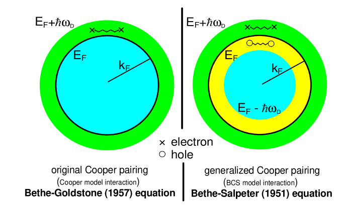
Figure 1: The Bethe-Goldstone equation (left) considers only 2e-CPs. The more general BS (right) includes 2h-CPs.

For the ideal-Fermi-gas-sea-based scenario for CPs when holes are not neglected, we assume the BCS model interaction $v(\left|\mathbf{k-k}^{\prime}\right|)=-V\theta_{BCS}(\epsilon_{\mathbf{k}})\theta_{BCS}(\epsilon_{\mathbf{k}^{\prime}})$ where $V\geq 0$ is the strength of the net attraction between pair partners and the unit step functions $\theta_{BCS}(\epsilon)$ restrict particle or hole energies $\epsilon_{k_{1}},$ $\epsilon_{k_{2}}$ to an energy interval of width $2\hbar\omega_{D}$ around the Fermi level $E_{F}$, namely $E_{F}\leq\epsilon_{\mathbf{k}_{1}},\epsilon_{\mathbf{k}_{2}}\leq E_{F}+\hbar\omega_{D}$ (for particles) and $E_{F}-\hbar\omega_{D}\leq\epsilon_{\mathbf{k}_{1}},\epsilon_{\mathbf{k}_{2}}\leq E_{F}$ (for holes). Integration over energies in (3) can then be evaluated directly in the complex $E^{\prime}$-plane resulting in the following equation for the wavefunction $\varphi_{\mathbf{k}}$ with zero CMM $\mathbf{K}=0$ that is

$$\varphi_{\mathbf{k}}=\frac{V}{L^{d}}\sum_{\mathbf{k}^{\prime}}{}^{{}^{\prime}}\frac{1}{(2\epsilon_{\mathbf{k}^{\prime}}-2E_{F}-\mathcal{E}_{0})}\varphi_{\mathbf{k}^{\prime}}-\frac{V}{L^{d}}\sum_{\mathbf{k}^{\prime}}{}^{{}^{\prime\prime}}\frac{1}{(2\epsilon_{\mathbf{k}^{\prime}}-2E_{F}-\mathcal{E}_{0})}\varphi_{\mathbf{k}^{\prime}}$$ (5)

where $\mathcal{E}_{0}$ is the $\mathbf{K}=0$ eigenvalue energy. The single prime over the first (2e-CP) summation term denotes the restriction $E_{F}<\epsilon_{\mathbf{k}^{\prime}}<E_{F}+\hbar\omega_{D}$ while the double prime in the last (2h-CP) term means $E_{F}-\hbar\omega_{D}<\epsilon_{\mathbf{k}^{\prime}}<E_{F}$. The ordinary Cooper (or BG) problem is compared in Fig. 1 with the BS problem where electron-hole symmetry is restored through inclusion of 2h-CPs, represented by the second term of (5), in addition to the 2e-CPs. Ignoring the second term of (5) gives the well-known solution [5]

$$\mathcal{E}_{0}^{C}=-2\hbar\omega_{D}/(e^{2/\lambda}-1)\quad\mathrel{\mathop{\longrightarrow}\limits_{\lambda\rightarrow 0}}\quad-2\hbar\omega_{D}\exp(-2/\lambda)$$ (6)

corresponding to a negative-energy, stationary-state bound 2e-CP, where $\lambda\equiv VN(E_{F})\geq 0$ with $N(E_{F})$ the electronic density of states for one spin. Note that a 2e-CP state for general CMM wavevector $\mathbf{K}$ of energy $\mathcal{E}_{K}^{C}$ is characterized only by a definite $K$ but not definite relative-momentum wavevector. This alone implies that ordinary, as well as the generalized CPs to be considered below, obey Bose statistics [6, 7]. Without the first summation term in (5) the same expression for the $\mathcal{E}_{0}^{C}$ of 2e-CPs follows for 2h-CPs, apart from an overall sign change.

Since (5) includes 2h-CPs along with 2e-CPs, eliminating the $\varphi_{\mathbf{k}}$’s from (5) leads to the BS eigenvalue equation for the pair energy $\mathcal{E}_{0}$

$$2/\lambda\,\,=\int\limits_{E_{F}}^{E_{F}+\hbar\omega_{D}}\frac{d\epsilon}{\epsilon-E_{F}-\mathcal{E}_{0}/2}\,\,-\int\limits_{E_{F}-\hbar\omega_{D}}^{E_{F}}\frac{d\epsilon}{\epsilon-E_{F}-\mathcal{E}_{0}/2}.$$ (7)

This is precisely Eq. (7-7) of Ref. [8] (where all energies are measured from the Fermi level) and in slightly different form than Eq. (33.2) of Ref. [9] before assuming that $\mathcal{E}_{0}$ is pure imaginary. If we assume that $\mathcal{E}_{0}$ can be real and $<0$ this eigenvalue refers to the 2e-CP “sector” in the BCS model interaction. In this case, the denominator in the first term never vanishes since the pole lies below $E_{F}$. A similar argument holds on considering the 2h-CP sector when $\mathcal{E}_{0}>0$ and now ignoring the first integral.

However, if we consider both particles and holes simultaneously as in (7), then we must take into account that, if there exists a real binding energy, there is a pole in one or the other integration intervals depending on the sign of $\mathcal{E}_{0}$. If one assumes that $\mathcal{E}_{0}/2=i\alpha,$ as in [8] or in [9] with $\alpha$ real both integrals are now free of singularities and can be integrated directly to give

$$1=\frac{\lambda}{2}\left\{\ln\frac{\hbar\omega_{D}-i\alpha}{-i\alpha}-\ln\frac{-i\alpha}{-\hbar\omega_{D}-i\alpha}\right\}=\frac{\lambda}{2}\ln\left[\frac{\hbar^{2}\omega_{D}^{2}+\alpha^{2}}{\alpha^{2}}\right].$$ (8)

This yields the well-known pair of purely-imaginary roots reported in Refs. [8, 9, 10], namely

$$\mathcal{E}_{0}^{BS}=\pm i2\hbar\omega_{D}/\sqrt{\exp(2/\lambda){-1}}\quad\mathrel{\mathop{\longrightarrow}\limits_{\lambda\rightarrow 0}}\quad\pm i2\hbar\omega_{D}\exp(-1/\lambda)\equiv\pm i\lim_{\lambda\rightarrow 0}\Delta$$ (9)

where

$$\Delta=\hbar\omega_{D}/\sinh(1/\lambda)$$ (10)

is the zero-temperature BCS energy gap [11].

A more general solution $\mathcal{E}_{0}$ can be obtained by assuming, without loss of generality, that it be complex, namely

$$\mathcal{E}_{0}\equiv r\exp i\phi$$ (11)

in (7). Then, direct integration in both terms of (7) yields

$$\frac{2}{\lambda}=\ln\frac{\mathcal{E}_{0}^{2}-(2\hbar\omega_{D})^{2}}{\mathcal{E}_{0}^{2}}\equiv\ln[\rho\exp i\theta]=\ln\rho+i\theta.$$ (12)

Defining

$$(2\hbar\omega_{D})^{2}/r^{2}\equiv\beta^{2}>0$$ (13)

and equating real and imaginary parts of (12) leads to

$$\mbox{a)}\quad\rho=\sqrt{1+\beta^{4}-2\beta^{2}\cos 2\phi}\qquad\mbox{and}\qquad\mbox{b)}\quad\theta=\tan^{-1}\frac{\beta^{2}\sin 2\phi}{1-\beta^{2}\cos 2\phi}.$$ (14)

Clearly, (12) means that

$$2/\lambda=\ln\rho\quad\quad\mbox{and}\quad\quad 0=\theta.$$ (15)

The last identity substituted in (14b) implies that $\beta^{2}\sin 2\phi=0$ which in turn is satisfied for

$$\phi=0,\,\pm\pi/2,\,\pm\pi,\,\pm 3\pi/2,\cdots.$$ (16)

Consider the solutions with $\phi=\pm\pi/2$ so that (14a) becomes $\rho=\sqrt{1+\beta^{4}+2\beta^{2}}=1+\beta^{2}>0.$ Thus, the first relation in (15) exponentiated gives $\exp(2/\lambda)=1+\beta^{2}$ and again recalling the definition (13) for $\beta$ as well as (11) leads to $\exp(-i\phi)\mathcal{E}_{0}\equiv r=2\hbar\omega_{D}/\sqrt{\exp(2/\lambda)-1}$ whereupon inserting $\phi=\pm\pi/2$ gives precisely (9).

However, if we take the first solution $\phi=0$ of (16) in (14a) this becomes $\rho=\sqrt{(1-\beta^{2})^{2}}=\left|1-\beta^{2}\right|.$ Since now $\mathcal{E}_{0}\equiv r$ and recalling (13) one obtains the real energy eigenvalues

$$\mathcal{E}_{0}^{BS}\,\mathcal{=\pm}\frac{2\hbar\omega_{D}}{\sqrt{\exp(2/\lambda)+1}}\quad\mathrel{\mathop{\longrightarrow}\limits_{\lambda\rightarrow 0}}\quad\pm 2\hbar\omega_{D}\exp(-1/\lambda)\equiv\pm\lim_{\lambda\rightarrow 0}\Delta.$$ (17)

In magnitude, this is always much larger than (6) since $e^{-1/\lambda}\gg e^{-2/\lambda}$ as $\lambda\rightarrow 0$. In Fig. 2 we plot the ratio $\mathcal{E}_{0}^{BS}/\mathcal{E}_{0}^{C}$ of the exact (17) to the exact (6) (upper curve); the ratio $\Delta/\mathcal{E}_{0}^{BS}$ of exact BCS gap $\Delta$ (10) to real BS binding energy $\mathcal{E}_{0}^{BS}$ found here (lower full curve); dashed curve is ratio of exact $\Delta$ to its weak-coupling limit, rhs of (10). Even for $\lambda$ as large as $1/2$ (the Migdal upper limit [12], marked as thin vertical line; see also Ref. [13] p. 204.) this ratio is only about $1.019$. Successive values $\pm\pi,$ $\pm 3\pi/2,\cdots$ for $\phi$ in (16) give nothing new. Solutions (9) are the well-known imaginary roots of the BS integral equation in the ladder approximation; they have been reported in Refs. [8, 9, 10]. The purely real energies (17) found here appear to be new.

Figure 2: Bottom: Ratio of exact BCS gap $\Delta$ (10) to real BS binding energy found here (lower full curve). Dashed curve is ratio of exact $\Delta$ to its weak-coupling limit, extreme rhs of (10). Upper full curve is ratio of real exact $\mathcal{E}_{0}^{BS}$ (17) to exact $\mathcal{E}_{0}^{C}$ (6). Horizontal thin dashed line marks drastic scale change. Vertical thin line is the Migdal upper limit [12] on $\lambda$.

In summary, we find real solutions for the binding energy of a “generalized” Cooper pair when the underlying BCS-type interaction is allowed to act between pairs of holes as well as of electrons through a Bethe-Salpeter equation that restores particle-hole symmetry around the Fermi level. The magnitude of the binding energy coincides with the BCS energy gap in the weak coupling regime. Finally, we note that the correct physical CP binding energies $\pm 2\Delta$ instead of $\pm\Delta$, follow when the ideal-Fermi-gas sea is replaced by a BCS-correlated sea, as in Ref. [3] Eqs. (12) and (13).

Acknowledgments MF, MdeLl and MAS acknowledge UNAM-DGAPA-PAPIIT (Mexico) for grants IN106401 & IN114708, and CONACyT (Mexico) grants 41302F and 43234F, for partial support.

References

• [1] E.E. Salpeter and H.A. Bethe, Phys. Rev. 84, 1232 (1951).
• [2] A.L. Fetter and J.D. Walecka, Quantum Theory of Many-Particle Systems (McGraw-Hill, New York, 1971).
• [3] M. Fortes, M.A. Solís, M. de Llano, and V.V. Tolmachev, Physica C 364, 95 (2001).
• [4] H.A. Bethe and J. Goldstone, Proc. Roy. Soc. (London) A 238, 551 (1957).
• [5] L.N. Cooper, Phys. Rev. 104, 1189 (1956).
• [6] M. de Llano, F.J. Sevilla, and S. Tapia, Int. J. Mod. Phys. B 20, 2931 (2006).
• [7] M. de Llano and J.J. Valencia, Mod. Phys. Lett. B 20, 1067 (2006).
• [8] J.R. Schrieffer, Theory of Superconductivity (Benjamin, Reading, MA, 1983) p. 168.
• [9] A.A. Abrikosov, L.P. Gorkov, and I.E. Dzyaloshinskii, Methods of Quantum Field in Statistical Physics (Dover, NY, 1975) § 33.
• [10] N.N. Bogoliubov, V.V. Tolmachev, and D.V. Shirkov, A New Method in the Theory of Superconductivity (Consultants Bureau, NY, 1959) p. 44.
• [11] J. Bardeen, L.N. Cooper, and J.R. Schrieffer, Phys. Rev. 106, 162 and 108, 1175 (1957).
• [12] A.B. Migdal, JETP 7, 996 (1958).
• [13] J.M. Blatt, Theory of Superconductivity (Academic, New York, 1964).