Existence, multiplicity and stability of endemic states for an age-structured S–I epidemic model

Abstract

We study an S–I type epidemic model in an age-structured population, with mortality due to the disease. A threshold quantity is found that controls the stability of the disease-free equilibrium and guarantees the existence of an endemic equilibrium. We obtain conditions on the age-dependence of the susceptibility to infection that imply the uniqueness of the endemic equilibrium. An example with two endemic equilibria is shown. Finally, we analyse numerically how the stability of the endemic equilibrium is affected by extra-mortality and by the possible periodicities induced by the demographic age-structure.

1 Introduction

In this paper we study the existence and uniqueness or multiplicity of positive steady states for an S–I type epidemic through an age-structured population. The population growth is subject to intra-specific mechanisms that, in the absence of infection, lead to a steady state which can be destabilised by Hopf bifurcation, for some values of the intrinsic reproduction number $R_{0}^{d}$. The infection is regulated by an age-dependent contact mechanism and interferes with the demographic process introducing additional mortality due to the disease.

A model with disease-induced mortality was for the first time introduced in [1] and the formulation in an age-structured context is due to May in [16]. In [2] Andreasen analysed two different cases: an age-structured epidemiological model and a model where infection has a constant duration. For the former he assumed that only the epidemiological interactions are density-dependent; he obtained conditions for the existence of one endemic state and studied its stability in the hypothesis that only fecundity is age dependent.

Here we give conditions for existence and uniqueness of an endemic equilibrium. A situation where two endemic equilibria appear is shown. Multiple solutions are specific of this model, in the sense that they do not occur in models without age structure or in the same model without the extra-mortality. Models with multiple steady states had already been proposed in the literature, the current model exhibits a different mechanism through which they arise. In particular, in [12] the role of variable population size in a multigroup epidemic model is emphasised, showing that multiple endemic equilibria are possible. Concerning the analysis of epidemic models with multiple endemic equilibria in an SIS epidemic model without age structure, see also [15] and the bibliography therein.

In addition to the study of existence of equilibria, we also investigate their stability showing that the effect of disease-induced mortality may produce stability changes related to Hopf’s bifurcation. Using a numerical method exposed in [3], we explore the behaviour of our model, within some critical parameter regions.

The paper is structured as follows. Next section is devoted to present our model, while in Section 3 the well-posedness of the system of partial differential equations is pointed out. In Section 4 conditions for existence of endemic equilibria are found. Successively, in Section 5 uniqueness versus multiplicity of endemic states is discussed.

In Section 6 the characteristic equation is computed, so that in Section 7 the stability analysis of the disease-free equilibrium is carried out and in Section 8 a stability change is described.

Finally, in Section 9 stability is numerically analysed in two different situations: where multiple endemic states occur and where periodic solutions arise through Hopf’s bifurcation. Our analysis reveals the importance of the parameter of disease-induced mortality. In the last section conclusions are drawn.

2 The model

We consider a population that, in the absence of infection is described by $N(a,t)$, the age density at time $t\geq 0$, where $a\in[0,a^{\dagger}]$, $a^{\dagger}<+\infty$ being the maximum age an individual of the population may reach. The growth of the population is regulated by the following model of Gurtin-MacCamy type (see [10])

$$\left\{\begin{aligned} &\frac{\partial N}{\partial t}+\frac{\partial N}{\partial a}+\mu(a)N(a,t)=0\,,\\ &N(0,t)=R_{0}^{d}\Phi(Q(t))\int_{0}^{a^{\dagger}}\beta(a)N(a,t)\,da\,.\end{aligned}\right.$$ (2.1)

In (2.1), $\beta(a)$ and $\mu(a)$ are the intrinsic vital rates, with $\beta$ normalised to satisfy

$$\int_{0}^{a^{\dagger}}\beta(\sigma)\pi(\sigma)\,d\sigma=1\,,$$

where

$$\pi(a)=e^{-\int_{0}^{a}\mu(\sigma)\,d\sigma}$$

is the survival probability, i.e. the probability at birth of surviving to age $a$. Moreover, the parameter $R_{0}^{d}$ is the demographic basic reproduction ratio and we suppose that

$$R_{0}^{d}>1\,.$$

The function $\Phi$ is a Lipschitz-continuous non-increasing function describing density-dependence of births. We assume that

$$\Phi(0)=1\,,\qquad\lim_{x\to+\infty}\Phi(x)=0$$

and that there exists $x_{0}\in{\mathbb{R}}$ such that $\Phi(x_{0})<1/R_{0}^{d}$ and $\Phi(\cdot)$ is decreasing on $[0,x_{0}]$. Finally, $Q$ is the size

$$Q(t)=\int_{0}^{a^{\dagger}}r(\sigma)N(\sigma,t)\,d\sigma,$$ (2.2)

where $r(a)$ is a weight kernel. We point out that, by the assumptions made, equation

$$R_{0}^{d}\Phi(Q_{d})=1$$ (2.3)

has a unique solution $Q_{d}^{*}$, providing a non trivial equilibrium

$$N^{*}(a)=\frac{Q_{d}^{*}\pi(a)}{\int_{0}^{a^{\dagger}}r(\sigma)\,\pi(\sigma)\,d\sigma}$$ (2.4)

of the population.

We recall (see [13]) that, provided that $\Phi$ is differentiable at $Q^{*}_{d}$, the stability of this steady state is related to the characteristic equation

$$1=\int_{0}^{a^{\dagger}}e^{-\lambda a}\beta(a)\pi(a)da+R_{0}^{d}\phi^{\prime}(Q_{d}^{*})N^{*}(0)\int_{0}^{a^{\dagger}}e^{-\lambda a}r(a)\pi(a)da\,,$$ (2.5)

the analysis of which also provides information about possible bifurcation points.

For the problem above we make the following standard hypotheses:

$$\beta(\cdot)\in L^{\infty}(0,a^{\dagger}), \beta(a)\geq 0\mbox{ in }[0,a^{\dagger}],$$

$$\mu(\cdot)\in L^{1}_{\mbox{loc}}(0,a^{\dagger}), \mu(a)\geq 0\mbox{ in }[0,a^{\dagger}],$$

$$r(\cdot)\in L^{\infty}(0,a^{\dagger}), r(a)\geq 0\mbox{ in }[0,a^{\dagger}]\,.$$

Since no individual may live past age $a^{\dagger}$, in order to have

$$\pi(a^{\dagger})=0,$$

we need to assume

$$\int_{0}^{a^{\dagger}}\mu(\sigma)\,d\sigma=+\infty\,.$$

The population develops an S–I type epidemics so that, denoting respectively by $S(a,t)$ and $I(a,t)$ the age-specific densities of susceptible and infective individuals at time $t$, the following system of equations describes the transmission dynamics of the disease:

$$\left\{\begin{aligned} &\frac{\partial S}{\partial t}+\frac{\partial S}{\partial a}=-\left(\lambda(a,t)+\mu(a)\right)S(a,t)\,,\\ &\frac{\partial I}{\partial t}+\frac{\partial I}{\partial a}=\lambda(a,t)\,S(a,t)-\left(\mu(a)+\alpha\right)I(a,t)\,,\\ &S(0,t)=R_{0}^{d}\Phi(Q(t))\int_{0}^{a^{\dagger}}\beta(a)\left(S(a,t)+I(a,t)\right)da\,,\\ &I(0,t)=0\,,\\ &S(a,0)=S_{0}(a)\geq 0\,,\\ &I(a,0)=I_{0}(a)\geq 0\,.\end{aligned}\right.$$ (2.6)

Here the terms $\lambda(a,t)$ and $\alpha$ describe the mechanism of infection. In particular, $\alpha$ is the extra-mortality due to the infection and $\lambda(a,t)$ is the force of infection. Concerning $Q(t)$, in (2.6) we set

$$Q(t)=\int_{0}^{a^{\dagger}}r(\sigma)(S(\sigma,t)+I(\sigma,t))\,d\sigma,$$ (2.7)

where we implicitly assume (compare with (2.2)) that both susceptible and infective individuals are equally active in the population. In fact, in (2.6) we are also assuming that newborns are all susceptible and equally produced by both kind of individuals. We note that the variable

$$N(a,t)=S(a,t)+I(a,t)$$

satisfies the equation

$$\frac{\partial N}{\partial t}+\frac{\partial N}{\partial a}+\mu(a)N(a,t)+\alpha I(a,t)=0\,,$$

showing how the disease-induced mortality affects the population growth.

For the parameters regulating the infection mechanism we assume that $\alpha\geq 0$ and consider the general separable inter-cohort form of the force of infection (see [4]):

$$\lambda(a,t)=K(a)\int_{0}^{a^{\dagger}}q(\sigma)\,I(\sigma,t)\,d\sigma\,,$$

where the age-specific infectiousness $q(\cdot)$ and the age-specific contagion rate $K(\cdot)$ satisfy the following conditions

$$q(\cdot),\,K(\cdot)\in L^{\infty}(0,a^{\dagger}),$$

$$q(a),\,K(a)\geq 0\mbox{ in }[0,a^{\dagger}]\,.$$

3 Well-posedness

Existence and uniqueness of a solution to problem (2.6) can be proved following the standard techniques presented for example in [13] (see also [17]). For the sake of completeness here we give a sketch of the proof without going into technical details. First we denote

$$B(t)=S(0,t)\,,$$ (3.1)

so that, integrating $S$ along the characteristics, we obtain

$$S(a,t)=\left\{\begin{array}[]{ll}S_{0}(a-t)e^{-\int_{0}^{t}[\lambda(a-t+\tau,\tau)+\mu(a-t+\tau)]\,d\tau}&\mbox{for }a\geq t\,,\\ B(t-a)\pi(a)e^{-\int_{0}^{a}\lambda(\sigma,t-a+\sigma)\,d\sigma}&\mbox{for }t\geq a\,.\end{array}\right.$$ (3.2)

Moreover, using (3.2) and integrating $I$ along the characteristics, we have

$$\begin{array}[]{l}I(a,t)=\\ \left\{\begin{array}[]{ll}e^{-\alpha t-\int_{0}^{t}\mu(a-t+\tau)\,d\tau}\left(I_{0}(a-t)\phantom{\int_{0}^{t}}\right.&\\ \quad\left.+S_{0}(a-t)\int_{0}^{t}\lambda(a-t+\tau,\tau)e^{\alpha\tau-\int_{0}^{\tau}\lambda(a-t+\xi,\xi)\,d\xi}d\tau\right)&\mbox{for }a\geq t\,,\\ \pi(a)e^{-\alpha a}B(t-a)\int_{0}^{a}\lambda(\sigma,t-a+\sigma)e^{\alpha\sigma-\int_{0}^{\sigma}\lambda(\rho,t-a+\rho)\,d\rho}d\sigma&\mbox{for }t\geq a\,.\end{array}\right.\end{array}$$ (3.3)

Then, if we denote

$$W(t)=\int_{0}^{a^{\dagger}}q(a)I(a,t)\,da\,,$$ (3.4)

we obtain that $B(t)$ satisfies the following integral equation (see (2.6)):

$$B(t)= R_{0}^{d}\Phi(Q(t))\left\{\int_{0}^{t}\beta(a)\pi(a)\Bigg{(}e^{-\alpha a}\right.$$ (3.5)

$$\left.+\alpha\int_{0}^{a}e^{-\alpha(a-\sigma)-\int_{0}^{\sigma}K(\rho)W(t-a+\rho)\,d\rho}\,d\sigma\right)B(t-a)\,da$$

$$+\int_{t}^{+\infty}\beta(a)\Bigg{[}S_{0}(a-t)\Bigg{(}e^{-\alpha t-\int_{0}^{t}\mu(a-t+\sigma)\,d\sigma}$$

$$+\alpha e^{-\int_{0}^{t}\mu(a-t+\sigma)\,d\sigma}\int_{0}^{t}e^{-\alpha(t-\sigma)-\int_{0}^{\sigma}K(a-t+\tau)\,W(\tau)\,d\tau}d\sigma\Bigg{)}$$

$$+I_{0}(a-t)e^{-\alpha t-\int_{0}^{t}\mu(a-t+\sigma)\,d\sigma}\Bigg{]}da\Bigg{\}}\,,$$

where all the functions are extended by zero outside the interval $[0,a^{\dagger}]$ and $Q$ is defined in (2.7). To solve our problem, we first consider $Q$ and $W$ as two given continuous, nonnegative functions. It is well known that equation (3.5), being a linear integral equation of Volterra type with a nonnegative kernel, admits a unique continuous and nonnegative solution. We denote it by $B(t,Q,W)$ to show the dependence on $Q$ and $W$.

Now, for a fixed $T>0$, we consider the space $E=C\left([0,T];(L^{1}(0,a^{\dagger}))^{2}\right)$ and the closed set

$$\mathcal{K}= \{k\in E\;|\;k(t)=(s(a,t),i(a,t)),\,s(a,t)\geq 0,\,i(a,t)\geq 0,$$

$$\|s(\cdot,t)\|_{L^{1}(0,a^{\dagger})}\leq M,\,\|i(\cdot,t)\|_{L^{1}(0,a^{\dagger})}\leq M\}\,,$$

with

$$M=(1+\alpha a^{\dagger})e^{R_{0}^{d}\|\beta\|_{L^{\infty}(0,a^{\dagger})}(1+\alpha a^{\dagger})T}\|S_{0}+I_{0}\|_{L^{1}(0,a^{\dagger})}\,.$$

Then, given $k\in E$, $k(t)=(s(a,t),i(a,t))$, we set

$$Q(t) = \int_{0}^{a^{\dagger}}r(a)\,(s(a,t)+i(a,t))\,da\,,$$

$$W(t) = \int_{0}^{a^{\dagger}}q(a)\,i(a,t)\,da\,,$$

and define the map

$$\mathcal{T}:\mathcal{K}\subset E\longrightarrow E\,,$$

where $\mathcal{T}(k)=(\tilde{s}(a,t),\tilde{\imath}(a,t))$ and

$$\tilde{s}(a,t) =\left\{\begin{array}[]{ll}S_{0}(a-t)e^{-\int_{0}^{t}[K(a-t+\sigma)W(\sigma)+\mu(a-t+\sigma)]\,d\sigma}&\mbox{for }a\geq t\,,\\ B(t-a,Q,W)\pi(a)e^{-\int_{0}^{a}K(\sigma)W(t-a+\sigma)\,d\sigma}&\mbox{for }t\geq a\,,\end{array}\right.$$

$$\tilde{\imath}(a,t) =\left\{\begin{array}[]{ll}e^{-\alpha t-\int_{0}^{t}\mu(a-t+\sigma)\,d\sigma}\left(I_{0}(a-t)\phantom{\int_{0}^{t}}+S_{0}(a-t)\cdot\right.&\\ \ \left.\cdot\int_{0}^{t}K(a-t+\sigma)W(\sigma)e^{\alpha\sigma-\int_{0}^{\sigma}K(a-t+\tau)W(\tau)\,d\tau}d\sigma\right)&\mbox{for }a\geq t\,,\\ \pi(a)e^{-\alpha a}B(t-a,Q,W)\cdot&\\ \ \cdot\int_{0}^{a}K(\sigma)W(t-a+\sigma)e^{\alpha\sigma-\int_{0}^{\sigma}K(\tau)W(t-a+\tau)\,d\tau}d\sigma&\mbox{for }t\geq a\,.\end{array}\right.$$

Standard estimates allow to prove that $\mathcal{T}$ sends $\mathcal{K}$ into itself and that a suitable power of $\mathcal{T}$ is a contraction, so that there exists a unique fixed point. Then, we can state the following result:

Theorem 3.1.

Let $(S_{0},I_{0})\in(L^{1}(0,a^{\dagger}))^{2}$, then there is one and only one $k\in\mathcal{K}$, $k(t)=(S(a,t),I(a,t))$ such that

$$S(a,t) =\left\{\begin{array}[]{ll}S_{0}(a-t)e^{-\int_{0}^{t}[K(a-t+\sigma)W(\sigma)+\mu(a-t+\sigma)]\,d\sigma}&\mbox{for }a\geq t\,,\\ B(t-a,Q,W)\pi(a)e^{-\int_{0}^{a}K(\sigma)W(t-a+\sigma)\,d\sigma}&\mbox{for }t\geq a\,,\end{array}\right.$$

$$I(a,t) =\left\{\begin{array}[]{ll}e^{-\alpha t-\int_{0}^{t}\mu(a-t+\sigma)\,d\sigma}\left(I_{0}(a-t)\phantom{\int_{0}^{t}}+S_{0}(a-t)\cdot\right.&\\ \ \left.\cdot\int_{0}^{t}K(a-t+\sigma)W(\sigma)e^{\alpha\sigma-\int_{0}^{\sigma}K(a-t+\tau)W(\tau)\,d\tau}d\sigma\right)&\mbox{for }a\geq t\,,\\ \pi(a)e^{-\alpha a}B(t-a,Q,W)\cdot&\\ \ \cdot\int_{0}^{a}K(\sigma)W(t-a+\sigma)e^{\alpha\sigma-\int_{0}^{\sigma}K(\tau)W(t-a+\tau)\,d\tau}d\sigma&\mbox{for }t\geq a\,,\end{array}\right.$$

$$Q(t) =\int_{0}^{a^{\dagger}}r(a)\,(S(a,t)+I(a,t))\,da\,,$$

$$W(t) =\int_{0}^{a^{\dagger}}q(a)\,I(a,t)\,da\,.$$

Moreover, the following properties hold:

• $\lim_{h\to 0}\frac{1}{h}[S(a+h,t+h)-S(a,t)]=-[K(a)W(t)+\mu(a)]S(a,t)$ a.e. in $[0,a^{\dagger}]\times{\mathbb{R}}^{+}$,

• $\lim_{h\to 0}\frac{1}{h}[I(a+h,t+h)-I(a,t)]=K(a)W(t)S(a,t)-[\mu(a)+\alpha]I(a,t)$ a.e. in $[0,a^{\dagger}]\times{\mathbb{R}}^{+}$,

• $\|S(\cdot,t)\|_{L^{1}(0,a^{\dagger})}\leq(1+\alpha a^{\dagger})e^{R_{0}^{d}\|\beta\|_{L^{\infty}(0,a^{\dagger})}(1+\alpha a^{\dagger})T}\|S_{0}+I_{0}\|_{L^{1}(0,a^{\dagger})}$,

• $\|I(\cdot,t)\|_{L^{1}(0,a^{\dagger})}\leq(1+\alpha a^{\dagger})e^{R_{0}^{d}\|\beta\|_{L^{\infty}(0,a^{\dagger})}(1+\alpha a^{\dagger})T}\|S_{0}+I_{0}\|_{L^{1}(0,a^{\dagger})}$,

• there exist two constants $C_{1},C_{2}>0$ depending on $M$ and $T$ such that

  $$\|k(t)-\tilde{k}(t)\|_{(L^{1}(0,a^{\dagger}))^{2}}\leq C_{1}e^{C_{2}t}\|(S_{0},I_{0})-(\tilde{S}_{0},\tilde{I}_{0})\|_{(L^{1}(0,a^{\dagger}))^{2}}$$

  where $\tilde{k}(t)$ is the solution relative to the initial datum $(\tilde{S}_{0},\tilde{I}_{0})$.

4 Search for endemic equilibria

We now consider the problem of existence of steady states for the system (2.6). Consequently, we are concerned with the problem

$$\left\{\begin{aligned} &\frac{dS^{*}}{da}=-\left(\lambda^{*}(a)+\mu(a)\right)S^{*}(a)\,,\\ &\frac{dI^{*}}{da}=\lambda^{*}(a)\,S^{*}(a)-\left(\mu(a)+\alpha\right)I^{*}(a)\,,\\ &S^{*}(0)=R_{0}^{d}\Phi(Q^{*})\int_{0}^{a^{\dagger}}\beta(a)\left(S^{*}(a)+I^{*}(a)\right)da\,,\\ &I^{*}(0)=0\,,\end{aligned}\right.$$

where

$$\lambda^{*}(a) = K(a)\int_{0}^{a^{\dagger}}q(\sigma)\,I^{*}(\sigma)\,d\sigma\,,$$

$$Q^{*} = \int_{0}^{a^{\dagger}}r(\sigma)\left(S^{*}(\sigma)+I^{*}(\sigma)\right)d\sigma\,.$$ (4.1)

It is easy to see that

$$S^{*}_{\mathrm{dfe}}(a)=N^{*}(a)\,,\qquad I^{*}_{\mathrm{dfe}}(a)\equiv 0$$ (4.2)

is the disease-free equilibrium, provided that $N^{*}(a)$ is given by (2.4). Then we concentrate on the search of endemic states, that is nonnegative solutions for which $I^{*}(a)$ does not vanish identically. Our aim in this Section is to reduce the solution of this problem to the solution of a system of equations of the scalar variables

$$B^{*} = S^{*}(0)\,,$$ (4.3)

$$W^{*} = \int_{0}^{a^{\dagger}}q(\sigma)\,I^{*}(\sigma)\,d\sigma\,.$$ (4.4)

To simplify, we denote

$$L(a)=\int_{0}^{a}K(\sigma)\,d\sigma\,$$ (4.5)

and, integrating, we obtain

$$S^{*}(a) =B^{*}e^{-WL(a)}\pi(a)\,,$$ (4.6)

$$I^{*}(a) =B^{*}W^{*}\pi(a)\int_{0}^{a}K(\sigma)e^{-W^{*}L(\sigma)-\alpha(a-\sigma)}\,d\sigma\,.$$

We define the following functions:

$$F(\alpha,W) = \int_{0}^{a^{\dagger}}\beta(\sigma)\pi(\sigma)\left(e^{-\alpha\sigma}+\alpha\int_{0}^{\sigma}e^{-WL(\rho)-\alpha(\sigma-\rho)}d\rho\right)d\sigma\,,$$

$$G(\alpha,W) = \int_{0}^{a^{\dagger}}r(\sigma)\pi(\sigma)\left(e^{-\alpha\sigma}+\alpha\int_{0}^{\sigma}e^{-WL(\rho)-\alpha(\sigma-\rho)}d\rho\right)d\sigma\,,$$

$$\ H(\alpha,W) = \int_{0}^{a^{\dagger}}q(\sigma)\pi(\sigma)\int_{0}^{\sigma}K(\rho)e^{-WL(\rho)-\alpha(\sigma-\rho)}d\rho\,d\sigma\,.$$

We note that, integrating by parts, $F(\alpha,W)$ and $G(\alpha,W)$ can be written as

$$F(\alpha,W) =\int_{0}^{a^{\dagger}}\beta(\sigma)\pi(\sigma)\left(e^{-WL(\sigma)}+W\int_{0}^{\sigma}K(\rho)e^{-WL(\rho)-\alpha(\sigma-\rho)}d\rho\right)d\sigma\,,$$ (4.7)

$$G(\alpha,W) =\int_{0}^{a^{\dagger}}r(\sigma)\pi(\sigma)\left(e^{-WL(\sigma)}+W\int_{0}^{\sigma}K(\rho)e^{-WL(\rho)-\alpha(\sigma-\rho)}d\rho\right)d\sigma\,.$$

Substituting (4.6) in (4.4) we get

$$W^{*} =B^{*}W^{*}\int_{0}^{a^{\dagger}}q(a)\pi(a)\int_{0}^{a}K(\sigma)e^{-W^{*}L(\sigma)-\alpha(a-\sigma)}d\sigma\,da$$ (4.8)

$$=B^{*}W^{*}H(\alpha,W^{*})\,.$$

Substituting (4.6) in (4.1), we have

$$Q^{*}=B^{*}\int_{0}^{a^{\dagger}}r(a)\pi(a)\left(e^{-W^{*}L(a)}+W^{*}\int_{0}^{a}K(\sigma)e^{-W^{*}L(\sigma)-\alpha(a-\sigma)}d\sigma\right)da$$

and, using (4.7) and (4.8),

$$Q^{*}=\frac{G(\alpha,W^{*})}{H(\alpha,W^{*})}\,.$$ (4.9)

Now our problem has been reduced to solving the following system of equations:

$$\left\{\begin{aligned} &B^{*}=\frac{1}{H(\alpha,W^{*})}\,,\\ &R_{0}^{d}\Phi\left(\frac{G(\alpha,W^{*})}{H(\alpha,W^{*})}\right)F(\alpha,W^{*})=1\,.\end{aligned}\right.$$ (4.10)

The second equation in (4.10) depends only on $W^{*}$: once we have a solution of it we can substitute it in the first equation. So, in order to simplify the second equation, we write

$$\varphi(\alpha,W)=R_{0}^{d}\Phi\left(\frac{G(\alpha,W)}{H(\alpha,W)}\right)F(\alpha,W)$$ (4.11)

and we are left with equation

$$\varphi(\alpha,W)=1\,.$$

We have that

$$\varphi(\alpha,0)=R_{0}^{d}\Phi\left(\frac{\int_{0}^{a^{\dagger}}r(\sigma)\pi(\sigma)\,d\sigma}{H(\alpha,0)}\right)$$

and

$$\lim_{x\to+\infty}\varphi(\alpha,x)=0\,,$$

so the second equation in (4.10) has at least one solution $W^{*}$ if $\varphi(\alpha,0)>1$. Since $\Phi(\cdot)$ is decreasing in $[0,Q^{*}_{d}]$, this latter condition is equivalent to

$$\frac{\int_{0}^{a^{\dagger}}r(\sigma)\pi(\sigma)\,d\sigma}{H(\alpha,0)}<Q_{d}^{*}\,,$$

where $Q_{d}^{*}$ is the solution of (2.3), that is to (see (2.4))

$$\frac{Q_{d}^{*}H(\alpha,0)}{\int_{0}^{a^{\dagger}}r(\sigma)\pi(\sigma)\,d\sigma}=N^{*}(0)H(\alpha,0)>1\,.$$ (4.12)

Condition (4.12) can be written as

$$R_{0}^{e}>1\,,$$ (4.13)

where $R_{0}^{e}$ is the basic epidemic reproduction ratio, i.e. the number of secondary cases which one case would produce in a completely susceptible population. This number is defined in this context as the spectral radius of the next-generation operator $\mathcal{G}$ (see [8], Chapter 7)

$$(\mathcal{G}u)(a)=\int_{0}^{a^{\dagger}}g(a,\sigma)\,u(\sigma)\,d\sigma\,,$$

where

$$g(a,\sigma)=\int_{\sigma}^{a^{\dagger}}K(a)q(\rho)N^{*}(a)\frac{\pi(\rho)}{\pi(\sigma)}e^{-\alpha(\rho-\sigma)}\,d\rho\,.$$

It is easy to see that

$$R_{0}^{e}=\int_{0}^{a^{\dagger}}K(a)N^{*}(a)\int_{a}^{a^{\dagger}}q(\sigma)\frac{\pi(\sigma)}{\pi(a)}e^{-\alpha(\sigma-a)}\,d\sigma\,da\,.$$

Since $N^{*}(0)=\frac{N^{*}(a)}{\pi(a)}$ for any $a\in[0,a^{\dagger}]$, we can write

$$N^{*}(0)H(\alpha,0)= \int_{0}^{a^{\dagger}}q(\sigma)\pi(\sigma)\int_{0}^{\sigma}K(a)e^{-\alpha(\sigma-a)}\frac{N^{*}(a)}{\pi(a)}da\,d\sigma$$

$$= \int_{0}^{a^{\dagger}}K(a)\frac{N^{*}(a)}{\pi(a)}\int_{a}^{a^{\dagger}}q(\sigma)\pi(\sigma)e^{-\alpha(\sigma-a)}d\sigma\,da=R_{0}^{e}\,.$$

Thus (4.13) is a sufficient condition for the existence of an endemic equilibrium.

Next section is devoted to discuss uniqueness of equilibria under such condition.

5 Discussing uniqueness of an endemic equilibrium

Condition (4.13) is sufficient to have at least one endemic state, but for uniqueness we need some additional assumptions. A first uniqueness case occurs when the disease does not induce mortality (see also [6]).

Theorem 5.1.

If $\alpha=0$ and $R_{0}^{e}>1$, there exists one and only one endemic equilibrium of the problem (2.6).

Proof.

Existence of endemic equilibria is equivalent to existence of solutions of the system (4.10). Since the function

$$\frac{\int_{0}^{a^{\dagger}}r(\sigma)\pi(\sigma)\,d\sigma}{\int_{0}^{a^{\dagger}}q(\sigma)\pi(\sigma)\int_{0}^{\sigma}K(\rho)e^{-WL(\rho)}d\rho\,d\sigma}$$

is increasing in $W$ and tends to infinity as $W$ tends to infinity, there exists $\widetilde{W}$ such that

$$\varphi(0,W)=\Phi\left(\frac{\int_{0}^{a^{\dagger}}r(\sigma)\pi(\sigma)\,d\sigma}{\int_{0}^{a^{\dagger}}q(\sigma)\pi(\sigma)\int_{0}^{\sigma}K(\rho)e^{-WL(\rho)}d\rho\,d\sigma}\right)\int_{0}^{a^{\dagger}}\beta(\sigma)\pi(\sigma)\,d\sigma$$

is decreasing for $W$ in $[0,\widetilde{W}]$, with $\varphi(0,\widetilde{W})<1$, and non-increasing for $W>\widetilde{W}$. Now, $R_{0}^{e}>1$ implies $\varphi(0,0)>1$ and so there exists one and only one solution of $\varphi(0,W)=1$. ∎

The proof of another condition for $\alpha>0$, requires the following Lemma (see [11])

Lemma 5.2 (Hadeler and Dietz).

Let $g$, $u$ and $v$ be locally summable real functions on the (finite or infinite) interval $(a,b)$, with $u(x),\,v(x)\geq 0$, such that

$$x\leq y\Longrightarrow g(x)\leq g(y)\quad\mbox{ and }\quad v(x)u(y)\geq u(x)v(y)\,.$$ (5.1)

Then

$$\int_{a}^{b}g(x)u(x)\,dx\cdot\int_{a}^{b}v(x)\,dx\geq\int_{a}^{b}g(x)v(x)\,dx\cdot\int_{a}^{b}u(x)\,dx\,,$$ (5.2)

provided the integrals exist.

Moreover, when $u$, $v$ and $g$ are positive and $\frac{u(x)}{v(x)}$ is strictly increasing, then (5.2) holds with strict inequality.

Then we obtain the following result.

Theorem 5.3.

If for any $0\leq\rho_{1}\leq\rho_{2}\leq a^{\dagger}$,

$$K(\rho_{1}) \int_{\rho_{1}}^{a^{\dagger}}q(\sigma)\pi(\sigma)e^{-\alpha\sigma}d\sigma\int_{\rho_{2}}^{a^{\dagger}}r(\sigma)\pi(\sigma)e^{-\alpha\sigma}d\sigma$$ (5.3)

$$\leq K(\rho_{2})\int_{\rho_{1}}^{a^{\dagger}}r(\sigma)\pi(\sigma)e^{-\alpha\sigma}d\sigma\int_{\rho_{2}}^{a^{\dagger}}q(\sigma)\pi(\sigma)e^{-\alpha\sigma}d\sigma\,.$$

and $R_{0}^{e}>1$, then there exists one and only one endemic equilibrium of the problem (2.6).

Proof.

Fixed $\alpha\geq 0$, $R_{0}^{e}>1$ implies $\varphi(\alpha,0)>1$. By definition $F(\alpha,W)$ is decreasing in $W$. Then, if we prove that $\frac{G(\alpha,W)}{H(\alpha,W)}$ is increasing in $W$, since $\lim_{W\to+\infty}\frac{G(\alpha,W)}{H(\alpha,W)}=+\infty$, we have that $\varphi(\alpha,\cdot)$ is decreasing on a suitable interval $[0,\widetilde{W}]$, where $\phi\left(\frac{G(\alpha,\widetilde{W})}{H(\alpha,\widetilde{W})}\right)>0$, and this gives our claim. Since

$$\frac{\partial}{\partial W}\left(\frac{G(\alpha,W)}{H(\alpha,W)}\right)=\frac{\frac{\partial G(\alpha,W)}{\partial W}H(\alpha,W)-G(\alpha,W)\frac{\partial H(\alpha,W)}{\partial W}}{(H(\alpha,W))^{2}}\,,$$

we study the sign of the numerator $G_{W}H-GH_{W}$. If we denote

$$u(\rho)=K(\rho)e^{-WL(\rho)+\alpha\rho}\int_{\rho}^{a^{\dagger}}q(\sigma)\pi(\sigma)e^{-\alpha\sigma}d\sigma$$

and

$$v(\rho)=e^{-WL(\rho)+\alpha\rho}\int_{\rho}^{a^{\dagger}}r(\sigma)\pi(\sigma)e^{-\alpha\sigma}d\sigma\,,$$

we get:

$$G_{W}H-GH_{W}= -\alpha\int_{0}^{a^{\dagger}}L(\rho)v(\rho)\,d\rho\,\int_{0}^{a^{\dagger}}u(\rho)\,d\rho$$

$$+\alpha\int_{0}^{a^{\dagger}}v(\rho)\,d\rho\,\int_{0}^{a^{\dagger}}L(\rho)u(\rho)\,d\rho$$

$$+\int_{0}^{a^{\dagger}}r(\sigma)\pi(\sigma)e^{-\alpha\sigma}d\sigma\,\int_{0}^{a^{\dagger}}L(\rho)u(\rho)\,d\rho\,.$$

Now we apply Hadeler-Dietz’s lemma. Since $L(\rho)$ by definition (see (4.5)) is increasing, we choose $g\equiv L$. The second part of condition (5.1) coincides with (5.3), so we obtain that

$$G_{W}H-GH_{W}\geq\int_{0}^{a^{\dagger}}r(\sigma)\pi(\sigma)e^{-\alpha\sigma}d\sigma\,\int_{0}^{a^{\dagger}}L(\rho)u(\rho)\,d\rho>0.$$

∎

Remark 5.4.

Condition (5.3) is verified for example when there exists a function $h(\cdot)$ such that $q(a)=h(a)r(a)$ and both $K(\cdot)$ and $h(\cdot)$ are non-decreasing functions.

We analyzed so far sufficient conditions to have uniqueness. We can also show examples in which multiple equilibria occur. The following case corresponds to a very special situation but it helps to understand the mechanisms responsible for non-uniqueness.

Let us consider the following choices

$$\begin{array}[]{l}a^{\dagger}=\frac{\pi}{2}\\ \alpha=10\\ R_{0}^{d}=27\\ \beta(a)\equiv 1\\ q(a)\equiv 1\\ \end{array}\hskip 56.9055pt\begin{array}[]{l}r(a)\equiv 1\\ \mu(a)=\tan a\\ K(a)=\left\{\begin{array}[]{ll}1&\mbox{if }a\in\left[0,\frac{\pi}{6}\right]\cup\left[\frac{\pi}{3},\frac{\pi}{2}\right]\\ 0&\mbox{if }a\in\left(\frac{\pi}{6},\frac{\pi}{3}\right)\end{array}\right.\\ \Phi(x)=\max\left\{1-\frac{x}{18},0\right\}\end{array}$$ (5.4)

Then we have

$$\pi(a)=\cos(a)\,,\qquad L(a)=\left\{\begin{array}[]{ll}a&\mbox{if }a\in\left[0,\frac{\pi}{6}\right],\\ \frac{\pi}{6}&\mbox{if }a\in\left(\frac{\pi}{6},\frac{\pi}{3}\right),\\ a-\frac{\pi}{6}&\mbox{if }a\in\left[\frac{\pi}{3},\frac{\pi}{2}\right].\end{array}\right.$$

Thus we may explicitly compute the functions $F$, $G$ and $H$ and we find that the function (see (4.11))

$$\varphi(10,W)=R_{0}^{d}\Phi\left(\frac{G(10,W)}{H(10,W)}\right)F(10,W)$$

has the graph shown in Figure 1. This leads to the following result

Theorem 5.5.

Problem (2.6) with the choices (5.4) has two endemic equilibria.

Figure 1: the graph of $\varphi(10,W)$ for the choices (5.4).

As an extension of this special case we consider the following forms

$$R_{0}^{d}=\frac{3X}{2}\quad\mbox{and}\quad\Phi(x)=\max\left\{1-\frac{x}{X},0\right\}$$ (5.5)

and in Figure 2 we show the endemic equilibria curves versus the parameter $\alpha$, for different choices of $X$. The special case of (5.4) corresponds to $X=18$. The behaviour becomes more evident as $X$ increases.

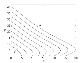
Figure 2: endemic equilibria curves for $X=10,14,18,22,26,30,34,38,42$ in (5.5).

6 Characteristic equation

In order to investigate the local asymptotic stability of the equilibria we consider the characteristic equation. For this standard technique see for example [13]. In the following sections we assume that $\Phi$ is differentiable at $Q^{*}_{d}$ (in the case of the disease free equilibrium) and in $Q^{*}$ defined in (4.1) (in the case of the endemic equilibria).

A convenient way to represent problem (2.6) in an equivalent form is to use the variables $B(t)$ as in (3.1) and $W(t)$ as in (3.4). In fact, using (3.2) and (3.3), we get a system of two integral equations that, for $t\geq a^{\dagger}$, is given by

$$\left\{\begin{aligned} B&(t)=R_{0}^{d}\Phi\left(\int_{0}^{a^{\dagger}}r(a)\pi(a)\left(e^{-\int_{0}^{a}K(\sigma)W(t-a+\sigma)\,d\sigma}\phantom{\int_{0}^{a}}\right.\right.\\ &\left.\left.+e^{-\alpha a}\int_{0}^{a}K(\sigma)e^{\alpha\sigma-\int_{0}^{\sigma}K(\rho)W(t-a+\rho)\,d\rho}W(t-a+\sigma)\,d\sigma\right)B(t-a)\,da\right)\cdot\\ &\cdot\int_{0}^{a^{\dagger}}\beta(a)\pi(a)\left(e^{-\int_{0}^{a}K(\sigma)W(t-a+\sigma)\,d\sigma}\phantom{\int_{0}^{a}}\right.\\ &\left.+e^{-\alpha a}\int_{0}^{a}K(\sigma)e^{\alpha\sigma-\int_{0}^{\sigma}K(\rho)W(t-a+\rho)\,d\rho}W(t-a+\sigma)\,d\sigma\right)B(t-a)\,da\,,\\ W&(t)=\int_{0}^{a^{\dagger}}q(a)\pi(a)e^{-\alpha a}\int_{0}^{a}K(\sigma)e^{\alpha\sigma-\int_{0}^{\sigma}K(\rho)W(t-a+\rho)\,d\rho}W(t-a+\sigma)\,d\sigma\cdot\\ &\cdot B(t-a)\,da\,.\end{aligned}\right.$$ (6.1)

Actually, the limiting equations of the two general integral equations for $B(t)$, $W(t)$ coincide with (6.1). Moreover, the constant solutions $B(t)\equiv B^{*}$, $W(t)\equiv W^{*}$ of (6.1) correspond to the different steady states of the problem. Namely we have:

• the trivial solution $B^{*}=W^{*}=0$;

• the disease-free equilibrium corresponding to $W^{*}=0$ and $B^{*}$ provided by the equation

  $$1=R_{0}^{d}\Phi\left(B^{*}\int_{0}^{a^{\dagger}}r(a)\pi(a)\,da\right);$$ (6.2)

• the endemic equilibria provided by system (4.10).

Note that the case of the disease-free equilibrium corresponds to (4.2) with (2.4) and (compare (6.2) with (2.3))

$$Q_{d}^{*}=B^{*}\int_{0}^{a^{\dagger}}r(a)\pi(a)\,da.$$ (6.3)

Finally, the endemic equilibrium is given by (4.6).

In order to linearise (6.1) at $(B^{*},W^{*})$, we let

$$b(t)=B(t)-B^{*}\quad\mbox{ and }\quad w(t)=W(t)-W^{*}\,.$$

Then we obtain the linear system

$$\left\{\begin{aligned} b(t)&=\int_{0}^{a^{\dagger}}\Psi_{1}(a)b(t-a)\,da+\int_{0}^{a^{\dagger}}\Psi_{2}(a)w(t-a)\,da\,,\\ w(t)&=\int_{0}^{a^{\dagger}}\Psi_{3}(a)b(t-a)\,da+\int_{0}^{a^{\dagger}}\Psi_{4}(a)w(t-a)\,da\,,\end{aligned}\right.$$ (6.4)

where the convolution kernels $\Psi_{1}$, $\Psi_{2}$, $\Psi_{3}$ and $\Psi_{4}$ are given by

$$\Psi_{1}(a)= \left(R_{0}^{d}\Phi(Q^{*})\beta(a)+B^{*}\frac{\Phi^{\prime}(Q^{*})}{\Phi(Q^{*})}r(a)\right)\cdot$$ (6.5)

$$\cdot\pi(a)\left(e^{-W^{*}L(a)}+W^{*}\int_{0}^{a}K(\sigma)e^{-\alpha(a-\sigma)-W^{*}L(\sigma)}d\sigma\right),$$

$$\Psi_{2}(a)= -\alpha B^{*}\int_{a}^{a^{\dagger}}\left(R_{0}^{d}\Phi(Q^{*})\beta(\sigma)+B^{*}\frac{\Phi^{\prime}(Q^{*})}{\Phi(Q^{*})}r(\sigma)\right)\pi(\sigma)K(\sigma-a)\cdot$$

$$\cdot\int_{\sigma-a}^{\sigma}e^{-\alpha(\sigma-\rho)-W^{*}L(\rho)}d\rho\,d\sigma\,,$$

$$\Psi_{3}(a)= W^{*}q(a)\pi(a)\int_{0}^{a}K(\sigma)e^{-\alpha(a-\sigma)-W^{*}L(\sigma)}d\sigma\,,$$

$$\Psi_{4}(a)= B^{*}\int_{a}^{a^{\dagger}}q(\sigma)\pi(\sigma)K(\sigma-a)\cdot$$

$$\cdot\left(e^{-\alpha a-W^{*}L(\sigma-a)}-W^{*}\int_{\sigma-a}^{\sigma}K(\rho)e^{-\alpha(\sigma-\rho)-W^{*}L(\rho)}d\rho\right)d\sigma\,,$$

with $Q^{*}$ defined in (4.1).

Taking Laplace transforms in (6.4), we obtain the following characteristic equation (see [13]):

$$\Psi(\lambda)=(1-\widehat{\Psi}_{1}(\lambda))(1-\widehat{\Psi}_{4}(\lambda))-\widehat{\Psi}_{2}(\lambda)\widehat{\Psi}_{3}(\lambda)=0\,,$$ (6.6)

where for $i=1,2,3,4$

$$\widehat{\Psi}_{i}(\lambda)=\int_{0}^{+\infty}e^{-\lambda a}\Psi_{i}(a)\,da$$

represents the Laplace transform of $\Psi_{i}(a)$.

To study the stability of an equilibrium, we need to determine the location of the roots of (6.6). In the following section we will be concerned with the disease-free equilibrium, then we will investigate the role of the parameter $\alpha$.

7 Stability of the disease-free equilibrium

In the case of the disease-free equilibrium (4.2), the convolution kernels become

$$\Psi_{1}(a)= \beta(a)\pi(a)+R_{0}^{d}B^{*}\Phi^{\prime}(Q^{*}_{d})\,r(a)\pi(a)\,,$$

$$\Psi_{2}(a)= B^{*}(e^{-\alpha a}-1)\int_{a}^{a^{\dagger}}\beta(\sigma)\pi(\sigma)K(\sigma-a)\,d\sigma$$

$$+R_{0}^{d}(B^{*})^{2}\Phi^{\prime}(Q^{*}_{d})\int_{0}^{a^{\dagger}}\beta(\sigma)\pi(\sigma)\,d\sigma(e^{-\alpha a}-1)\int_{a}^{a^{\dagger}}r(\sigma)\pi(\sigma)K(\sigma-a)\,d\sigma\,,$$

$$\Psi_{3}(a)= 0\,,$$

$$\Psi_{4}(a)= B^{*}e^{-\alpha a}\int_{a}^{a^{\dagger}}q(\sigma)\pi(\sigma)K(\sigma-a)\,d\sigma\,,$$

where $Q^{*}_{d}$ is given in (6.3).

Hence, the roots of (6.6) are the union of the roots of the two equations

$$\hat{\Psi}_{1}(\lambda)=1,\quad\hat{\Psi}_{4}(\lambda)=1,$$

that can be considered separately. Note that the first of this equations is exactly the characteristic equation (2.5) for the demographic problem (2.1) in the absence of the disease. Thus we have

Theorem 7.1.

If $R_{0}^{e}>1$, the disease-free equilibrium is unstable. If $R_{0}^{e}<1$, the disease-free equilibrium is stable or unstable depending on whether the equilibrium (2.4) of the population is stable or not for (2.1).

Proof.

Let $R_{0}^{e}>1$. We have that

$$\hat{\Psi}_{4}(0) =\int_{0}^{a^{\dagger}}\Psi_{4}(a)\,da=B^{*}\int_{0}^{a^{\dagger}}e^{-\alpha a}\int_{a}^{a^{\dagger}}q(\sigma)\pi(\sigma)K(\sigma-a)\,d\sigma\,da$$

$$=B^{*}H(\alpha,0)\,.$$

Since

$$\frac{G(\alpha,0)}{H(\alpha,0)}=\frac{Q^{*}_{d}}{N^{*}(0)H(\alpha,0)}<Q^{*}_{d}$$

and $\Phi(\cdot)$ is decreasing on $[0,Q^{*}_{d}]$, one has

$$\varphi(\alpha,0)=R_{0}^{d}\Phi\left(\frac{G(\alpha,0)}{H(\alpha,0)}\right)>1\,.$$

Now, comparing (6.2) with the previous equation, we get that

$$B^{*}>\frac{1}{H(\alpha,0)}$$

and consequently $\hat{\Psi}_{4}(0)>1$. This means that $1-\hat{\Psi}_{4}(t)$ has exactly one root on the positive real line.

If $R_{0}^{e}<1$, then $\hat{\Psi}_{4}(0)<1$ and, if $\lambda\in{\mathbb{C}}$ has positive real part,

$$|1-\hat{\Psi}_{4}(\lambda)| \geq 1-\left|\int_{0}^{a^{\dagger}}e^{-\lambda a}\Psi_{4}(a)\,da\right|$$

$$>1-\int_{0}^{a^{\dagger}}\Psi_{4}(a)\,da=1-\hat{\Psi}_{4}(0)>0\,.$$

So, there are no zeros of $1-\hat{\Psi}_{4}(\lambda)$ with positive real part. The study of the zeros of $1-\hat{\Psi}_{1}(\lambda)$ coincides with the stability analysis of the non trivial equilibrium of the total population (equation (2.1)) and this concludes the proof. ∎

From the previous Theorem we see that the epidemic reproduction ratio $R_{0}^{e}$ determines also stability of the disease free equilibrium. In the next Section we discuss how instability may depend on the disease induced mortality $\alpha$.

8 Destabilizing effect of the extra-mortality

Since an analytic study of the characteristic equation at the endemic equilibrium does not seem to be possible in the general case, we present a specific example. We consider a special set of parameters that shows how the extra-mortality $\alpha$ can destabilize the endemic equilibrium.

Let us first consider the following choices:

$$a^{\dagger}=\frac{\pi}{2}\,,\qquad\beta(a)=\frac{3}{2}\sin(2a)\,,\qquad r(a)=\frac{3}{2}\sin(2a)\,,\qquad\mu(a)=\tan a\,.$$ (8.1)

With these choices and $\alpha=0$ the convolution kernels (6.5) for the endemic equilibrium become

$$\Psi_{1}(a)= \left(1+R_{0}^{d}B^{*}\Phi^{\prime}(Q^{*})\right)\frac{3}{2}\sin(2a)\cos(a)\,,$$

$$\Psi_{2}(a)= 0\,,$$

$$\Psi_{3}(a)= q(a)\cos(a)\left(1-e^{-W^{*}L(a)}\right)\,,$$

$$\Psi_{4}(a)= B^{*}\int_{a}^{a^{\dagger}}q(\sigma)\cos(\sigma)K(\sigma-a)e^{-W^{*}L(\sigma)}d\sigma\,,$$

where $B^{*}$ and $Q^{*}$ are given by (4.10) and (4.9). Then we have the following result.

Proposition 8.1.

Let (8.1) be satisfied. If $\alpha=0$ and

$$R_{0}^{d}B^{*}\Phi^{\prime}(Q^{*})=-5\,,$$ (8.2)

then the characteristic equation (6.6) has two imaginary roots $\lambda_{\pm}=\pm 5i$ and any other root has negative real part.

Proof.

Since $\Psi_{2}(a)=0$, the characteristic equation is simply

$$\Psi(\lambda)=(1-\widehat{\Psi}_{1}(\lambda))(1-\widehat{\Psi}_{4}(\lambda))=0\,.$$

If $\lambda$ has nonnegative real part, we have

$$\left|\Re\left(\widehat{\Psi}_{4}(\lambda)\right)\right| \leq \left|B^{*}\int_{0}^{a^{\dagger}}e^{-\lambda a}\int_{a}^{a^{\dagger}}q(\sigma)\pi(\sigma)K(\sigma-a)e^{-W^{*}L(\sigma)}d\sigma\,da\right|$$

$$\leq B^{*}\int_{0}^{a^{\dagger}}\int_{a}^{a^{\dagger}}q(\sigma)\pi(\sigma)K(\sigma-a)e^{-W^{*}L(\sigma)}d\sigma\,da\,.$$

Since

$$\int_{0}^{a^{\dagger}} \int_{a}^{a^{\dagger}}q(\sigma)\pi(\sigma)K(\sigma-a)e^{-W^{*}L(\sigma)}d\sigma\,da=\int_{0}^{a^{\dagger}}q(\sigma)\pi(\sigma)e^{-W^{*}L(\sigma)}\int_{0}^{\sigma}K(\rho)\,d\rho\,d\sigma$$

$$<\int_{0}^{a^{\dagger}}q(\sigma)\pi(\sigma)\int_{0}^{\sigma}K(\rho)e^{-W^{*}L(\rho)}\,d\rho\,d\sigma=H(0,W^{*})=\frac{1}{B^{*}}\,,$$

$\left|\Re\left(\widehat{\Psi}_{4}(\lambda)\right)\right|<1$. Then the roots of the characteristic equation with nonnegative real part can be found only if $\widehat{\Psi}_{1}(\lambda)=1$, i.e.

$$(1+\tau)\frac{3}{2}\int_{0}^{\frac{\pi}{2}}e^{-\lambda a}\sin(2a)\cos(a)\,da=1$$ (8.3)

with $\tau=R_{0}^{d}B^{*}\Phi^{\prime}(Q^{*})$. We look for values of $\tau<0$ for which a couple of imaginary roots $\lambda=\pm i\omega$ of (8.3) exist. This is equivalent to solving the following system:

$$\left\{\begin{array}[]{l}\int_{0}^{\frac{\pi}{2}}\sin(\omega a)\sin(2a)\cos(a)\,da=0\,,\\ (1+\tau)\frac{3}{2}\int_{0}^{\frac{\pi}{2}}\cos(\omega a)\sin(2a)\cos(a)\,da=1\,.\end{array}\right.$$

The first equation gives

$$\frac{\sin\frac{\pi(\omega-3)}{2}}{4(\omega-3)}+\frac{\sin\frac{\pi(\omega-1)}{2}}{4(\omega-1)}-\frac{\sin\frac{\pi(\omega+1)}{2}}{4(\omega+1)}-\frac{\sin\frac{\pi(\omega+3)}{2}}{4(\omega+3)}=\frac{4\omega\cos\frac{\pi\omega}{2}}{(\omega^{2}-9)(\omega^{2}-1)}=0$$

and the solutions are $\omega_{k}^{\pm}=\pm(2k+1)$ with $k=2,3,\dots$. Correspondingly, the values of $\tau=\tau_{k}$ are given by the following equality

$$\tau_{k} =\frac{2}{3\int_{0}^{\frac{\pi}{2}}\cos((2k+1)a)\sin(2a)\cos(a)\,da}-1$$

$$=\frac{2}{\frac{3}{8}\left[\frac{\cos(2(k-1)a)}{k-1}+\frac{\cos(2ka)}{k}-\frac{\cos(2(k+1)a)}{k+1}-\frac{\cos(2(k+2)a)}{k+2}\right]_{0}^{\frac{\pi}{2}}}-1\,,$$

which means

$$\tau_{k}=\left\{\begin{array}[]{ll}\frac{1-4k^{2}}{3}&\mbox{for $k$ even}\,,\\ \frac{-4k^{2}-8k-3}{3}&\mbox{for $k$ odd}\,.\end{array}\right.$$

It is easy to verify that $\tau_{k}$ is decreasing with $k$. Then $\tau_{2}=-5$ is the maximum of the $\tau_{k}$’s. Since by the implicit function theorem one obtains that $\frac{\partial\Re\lambda}{\partial\tau}(-5)<0$, $\lambda=\omega_{2}^{\pm}i=\pm 5i$ are the first roots to cross the imaginary axis and this completes the proof. ∎

We now let $\alpha$ become positive, and analyze how the stability of the endemic equilibrium changes with $\alpha$. For simplicity we make a further choice considering

$$\Phi(x)=\max\left\{1-\frac{x}{10},0\right\}\,,\qquad q(a)=\frac{3}{2}\sin(2a)\,,\qquad K(a)=a\,.$$ (8.4)

By (8.1) and Remark 5.4, for every fixed $\alpha$ there exists one and only one endemic equilibrium. So, equation $\varphi(\alpha,W)=1$ has only one solution $(0,W^{*}_{0})$, with $\alpha=0$. With the choices made in (8.1), (8.2) and (8.4), we get

$$R_{0}^{d}=6\qquad\mbox{and}\qquad H(0,W^{*}_{0})=\frac{3}{25}\,.$$

so that $W^{*}_{0}\simeq 5.04512$. Moreover at this point we have $\displaystyle\frac{\partial\varphi(0,W^{*}_{0})}{\partial W}\neq 0$. Then for $\alpha>0$ sufficiently small, there exists a function $W^{*}(\alpha)$ such that

$$\varphi(\alpha,W^{*}(\alpha))=1$$ (8.5)

and we obtain a branch of endemic states $\left(B^{*}(\alpha),W^{*}(\alpha)\right)$.

Now we show that this endemic equilibrium changes its stability, in the sense that at $\alpha=0$ the roots of the characteristic equation cross forward the imaginary axis.

We write $\lambda=\zeta+i\omega$, so that we can consider the characteristic equation (6.6) at the equilibrium $\left(B^{*}(\alpha),W^{*}(\alpha)\right)$, as a system depending on $\alpha$

$$F_{1}(\alpha,\zeta,\omega) =\Re\Psi(\lambda)=0\,,$$

$$F_{2}(\alpha,\zeta,\omega) =\Im\Psi(\lambda)=0\,.$$

By Proposition 8.1 we know that $F_{1}(0,0,\pm 5)=F_{2}(0,0,\pm 5)=0$, while detailed calculations show

$$\frac{\partial F_{1}}{\partial\omega}(0,0,\pm 5) =-\frac{\partial F_{2}}{\partial\zeta}(0,0,\pm 5),$$

$$\frac{\partial F_{2}}{\partial\omega}(0,0,\pm 5) =\frac{\partial F_{1}}{\partial\zeta}(0,0,\pm 5),$$

so that the jacobian of the system with respect to $\zeta$ and $\omega$ at $(0,0,\pm 5)$ is equal to

$$\left(\frac{\partial{F_{1}}}{\partial\zeta}(0,0,\pm 5)\right)^{2}+\left(\frac{\partial F_{2}}{\partial\zeta}(0,0,\pm 5)\right)^{2}$$

and by numerical computation (the evaluations are obtained using Mathematica, www.wolfram.com) we conclude that it is positive. Then for $\alpha>0$ sufficiently small there exist $\zeta(\alpha)$ and $\omega(\alpha)$ such that $\zeta(0)=0$, $\omega(0)=\pm 5$ and $F_{i}(\alpha,\zeta(\alpha),\omega(\alpha))=0$ for $i=1,2$. Concerning the sign of $\zeta^{\prime}(0)$, again by numerical computation we have

$$\zeta^{\prime}(0)=\frac{-\frac{\partial F_{1}}{\partial\alpha}(0,0,\pm 5)\frac{\partial F_{1}}{\partial\zeta}(0,0,\pm 5)-\frac{\partial F_{2}}{\partial\alpha}(0,0,\pm 5)\frac{\partial F_{2}}{\partial\zeta}(0,0,\pm 5)}{\left(\frac{\partial F_{1}}{\partial\zeta}(0,0,\pm 5)\right)^{2}+\left(\frac{\partial F_{2}}{\partial\zeta}(0,0,\pm 5)\right)^{2}}>0$$

and we conclude that, in this example, disease-induced mortality yields instability.

The calculations to obtain the conclusion above are standard, but for the reader’s convenience we give below some details. With the choices made in this special case we have the following kernels where we have highlighted the dependence on $\alpha$

$$\Psi_{1}(\alpha,a)= \left(6\Phi(Q^{*}(\alpha))-\frac{B^{*}(\alpha)}{10\Phi(Q^{*}(\alpha))}\right)\frac{3}{2}\sin(2a)\cos(a)\cdot$$

$$\cdot\left(e^{-\alpha a}+\alpha\int_{0}^{a}e^{-\alpha(a-\sigma)-\frac{W^{*}(\alpha)}{2}\sigma^{2}}d\sigma\right)\,,$$

$$\Psi_{2}(\alpha,a)= -\alpha B^{*}(\alpha)\left(6\Phi(Q^{*}(\alpha))-\frac{B^{*}(\alpha)}{10\Phi(Q^{*}(\alpha))}\right)\frac{3}{2}\cdot$$

$$\cdot\int_{a}^{\frac{\pi}{2}}\sin(2\sigma)\cos(\sigma)(\sigma-a)\int_{\sigma-a}^{\sigma}e^{-\alpha(\sigma-\rho)-\frac{W^{*}(\alpha)}{2}\rho^{2}}d\rho\,d\sigma\,,$$

$$\Psi_{3}(\alpha,a)= W^{*}(\alpha)\frac{3}{2}\sin(2a)\cos(a)\int_{0}^{a}\sigma e^{-\alpha(a-\sigma)-\frac{W^{*}(\alpha)}{2}\sigma^{2}}d\sigma$$

$$\Psi_{4}(\alpha,a)= B^{*}(\alpha)\frac{3}{2}\int_{a}^{\frac{\pi}{2}}\sin(2\sigma)\cos(\sigma)(\sigma-a)\cdot\,,$$

$$\cdot\left(e^{-\frac{W^{*}(\alpha)}{2}\sigma^{2}}-\alpha\int_{\sigma-a}^{\sigma}e^{-\alpha(\sigma-\rho)-\frac{W^{*}(\alpha)}{2}\rho^{2}}d\rho\right)d\sigma\,.$$

Then we evaluate the following derivatives (they are the only derivatives we need)

$$\frac{\partial\Psi_{1}}{\partial\alpha}(0,a) =\sin(2a)\cos(a)\left(-3W^{*}(0)+6a-6\int_{0}^{a}e^{-\frac{W^{*}(0)}{2}\sigma^{2}}d\sigma\right),$$

$$\frac{\partial\Psi_{2}}{\partial\alpha}(0,a) =50\int_{a}^{\frac{\pi}{2}}\sin(2\sigma)\cos(\sigma)(\sigma-a)\int_{\sigma-a}^{\sigma}e^{-\frac{W^{*}(0)}{2}\rho^{2}}d\rho\,d\sigma\,,$$

where we have used

$${W^{*}}^{\prime}(0)=\left(\frac{12}{125}W^{*}(0)-1\right)\frac{\frac{\partial H}{\partial\alpha}(0,W^{*}(0)}{\frac{\partial H}{\partial W}(0,W^{*}(0))}\,,$$

obtained by Dini’s Theorem applied to (8.5). The above expressions are used to compute the following quantities

$$A =1-\int_{0}^{\frac{\pi}{2}}\cos(5a)\Psi_{4}(0,a)\,da\simeq 0.83432,$$

$$B =\int_{0}^{\frac{\pi}{2}}\sin(5a)\Psi_{4}(0,a)\,da\simeq 0.236031,$$

$$C =\int_{0}^{\frac{\pi}{2}}\cos(5a)\frac{\partial\Psi_{1}}{\partial\alpha}(0,a)da\simeq 2.52632,$$

$$D =\int_{0}^{\frac{\pi}{2}}\sin(5a)\frac{\partial\Psi_{1}}{\partial\alpha}(0,a)da\simeq-0.397545,$$

$$E =\int_{0}^{\frac{\pi}{2}}\cos(5a)\Psi_{3}(0,a)\,da\simeq-0.147547,$$

$$F =\int_{0}^{\frac{\pi}{2}}\sin(5a)\Psi_{3}(0,a)\,da\simeq-0.177344,$$

$$G =\int_{0}^{\frac{\pi}{2}}\cos(5a)\frac{\partial\Psi_{2}}{\partial\alpha}(0,a)da\simeq-0.0744986,$$

$$H =\int_{0}^{\frac{\pi}{2}}\sin(5a)\frac{\partial\Psi_{2}}{\partial\alpha}(0,a)da\simeq-0.249824,$$

that finally allow us to evaluate

$$\frac{\partial F_{1}}{\partial\alpha}(0,0,\pm 5) =-AC-BD-EG+FH\simeq-1.98062,$$

$$\frac{\partial F_{2}}{\partial\alpha}(0,0,\pm 5) =\pm\left(-BC+AD+FG+EH\right)\simeq\mp 0.877897,$$

$$\frac{\partial F_{1}}{\partial\zeta}(0,0,\pm 5) =\frac{5\pi}{32}A+\frac{2}{3}B\simeq 0.5669,$$

$$\frac{\partial F_{2}}{\partial\zeta}(0,0,\pm 5) =\pm\left(\frac{5\pi}{32}B-\frac{2}{3}A\right)\simeq\mp 0.440352,$$

so that $\zeta^{\prime}(0)\simeq 1.42878>0$.

9 Numerical exploration

In the previous Section we have produced an example showing that the parameter $\alpha$, representing disease-induced mortality, can actually modify the dynamics of the system and that periodic solutions are possible via Hopf bifurcation. In order to explore the model in a systematic way, we now resort to a numerical method that allows to determine the roots of the characteristic equation and follow their displacement as $\alpha$ varies. The method, proposed in [3], provides numerical approximations to the rightmost part of the characteristic spectrum associated to the model linearized around the equilibrium to be investigated. It is indeed well-known that the zero solution of this latter is asymptotically stable if and only if all the characteristic roots have strictly negative real part.

The numerical scheme developed in [3] is actually devoted to the stability analysis of the scalar Gurtin-MacCamy model [10], but it can be extended straightforwardly to the $m$-dimensional system ($m\geq 1$)

$$\left\{\begin{aligned} &\frac{\partial{\bf P}}{\partial t}+\frac{\partial{\bf P}}{\partial a}+\mathcal{M}(a,{\bf S}(t)){\bf P}(a,t)=0\,,\\ &{\bf P}(0,t)=\int_{0}^{a^{\dagger}}\mathcal{B}(a,{\bf S}(t)){\bf P}(a,t)da\,,\\ &{\bf S}(t)=\int_{0}^{a^{\dagger}}\mathcal{G}(a){\bf P}(a,t)da\,,\\ &{\bf P}(a,0)={\bf P_{0}}(a),\end{aligned}\right.$$ (9.1)

where ${\bf P}:[0,a^{\dagger}]\times[0,+\infty)\rightarrow\mathbb{R}^{m}$ is the $m$-vector of population densities, $\mathcal{M},\mathcal{B}:[0,a^{\dagger}]\times\mathbb{R}^{n}\rightarrow\mathbb{R}^{m\times m}$ are the matrices of mortality and fertility rates, respectively, and ${\bf S}:[0,+\infty)\rightarrow\mathbb{R}^{n}$ ($n\geq 1$) is the $n$-vector of population sizes, i.e. a selection of $n$ homogeneous population sub-classes through the weight function $\mathcal{G}:[0,a^{\dagger}]\rightarrow\mathbb{R}^{n\times m}$.

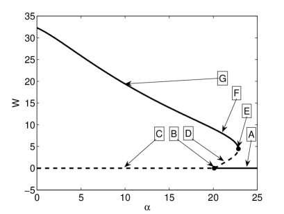
Figure 3: bifurcation diagram of equilibrium $W^{\ast}$ as $\alpha$ varies ($X=34$ in (5.5)).

The epidemic model (2.6) we are interested in fits into (9.1) by choosing $m=2$, $n=2$, the population vector

$${\bf P}(a,t)=\left(S(a,t),I(a,t)\right)^{T}$$

and the size vector

$${\bf S}(t)=\left(Q(t),W(t)\right)^{T},$$

which corresponds to selecting

$$\mathcal{G}(a)=\begin{pmatrix}r(a)&r(a)\\ 0&q(a)\\ \end{pmatrix}.$$

Moreover, the matrices relative to the vital rates are given by

$$\mathcal{M}(a,{\bf S}(t))=\begin{pmatrix}K(a)W(t)+\mu(a)&0\\ -K(a)W(t)&\alpha+\mu(a)\\ \end{pmatrix}$$

and

$$\mathcal{B}(a,{\bf S}(t))=\begin{pmatrix}R_{0}^{d}\beta(a)\Phi(Q(t))&R_{0}^{d}\beta(a)\Phi(Q(t))\\ 0&0\\ \end{pmatrix}.$$

Within this framework we consider the special choices of Section 5, namely (5.4) and (5.5) with $X=34$, letting $\alpha$ vary along the corresponding equilibrium curve represented in Figure 2 (the third curve from the right). For each point on the curve (included those corresponding to the disease-free equilibrium for $W^{\ast}=0$) we are able to compute the rightmost characteristic root (rounded to machine precision, see [3]) and thus to say whether the corresponding equilibrium is locally asymptotically stable or not. The overall situation is illustrated in Figure 3 where solid lines denote stability and dashed lines denote instability.

We start our analysis from the right hand branch of the disease free equilibrium by investigating, for instance, the spectrum for $\alpha=24$ (A in Figure 3 and Figure 4): the rightmost roots have negative real part and hence the trivial equilibrium is stable. By decreasing $\alpha$ the real root moves to the right until at $\alpha=\alpha_{1}\simeq 20.1143$ it crosses the imaginary axis rightward (B). This first bifurcation makes the trivial equilibrium lose its stability and a branch of endemic equilibria raises. Following the disease-free branch by further decreasing $\alpha$ it is confirmed that the instability persists (C, $\alpha=10$).

Going back to the bifurcation point at $\alpha_{1}$, we now follow the endemic branch by increasing $\alpha$. The branch is unstable (D, $\alpha=21$) until at $\alpha=\alpha_{2}\simeq 22.8495$ the leading root crosses the imaginary axis leftward (E).

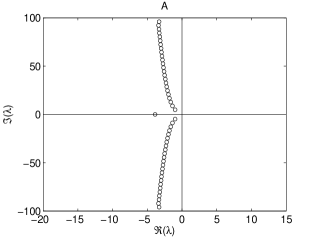
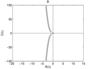
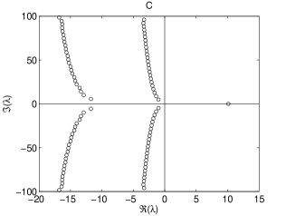
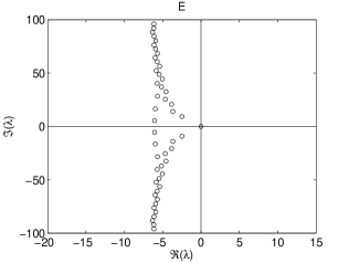
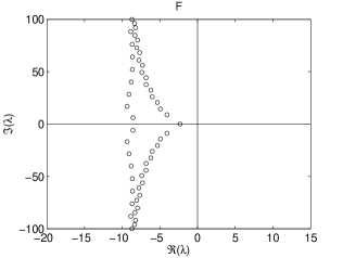
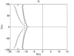
Figure 4: relevant characteristic roots for different equilibrium points, referring to the bifurcation diagram of Figure 3 ($X=34$ in (5.5)).

This second bifurcation makes the endemic equilibrium gain back its stability. Then the branch continues by decreasing $\alpha$ again and at $\alpha=21$ (F) the second endemic equilibrium is stable opposite to the first one for the same value of $\alpha$ (D). The branch remains stable by further decreasing $\alpha$ (F, $\alpha=10$).

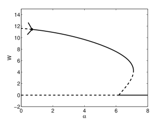
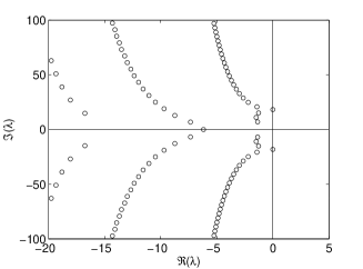
Figure 5: bifurcation diagram of equilibrium $W^{\ast}$ as $\alpha$ varies (left) and relevant characteristic roots (right) for $\alpha\simeq 0.6743$, value at which a Hopf bifurcation occurs (black dot in the left figure).

Similar trends are obtained for other values of $X$ for which double endemic equilibria exist. On the other side, for those values of $X$ for which only one endemic equilibrium exists (for instance $X=10,14$ in Figure 2), it can be observed by the roots computation that at the first bifurcation the disease-free equilibrium loses its stability in favour of the endemic one. This latter then preserves its stability for decreasing values of $\alpha$ down to $\alpha=0$.

As a consequence of the destabilisation shown in Section 8, it is possible that under different choices of the parameters a Hopf bifurcation occurs. In fact, if we consider the same choices made in (5.4) for $a^{\dagger}$ and $K$, but set

$$\begin{array}[]{l}\beta(a)=\frac{3}{2}\sin{(2a)}\,,\\ q(a)=\sin{(2a)}\,,\\ r(a)=\frac{3}{2}\sin{(2a)}\,,\end{array}\hskip 56.9055pt\begin{array}[]{l}\mu(a)=\tan a\,,\\ \Phi(x)=\max\{1-\frac{x}{18},0\}\,,\end{array}$$ (9.2)

we get the bifurcation diagram represented in Figure 5 (left). The black dot, corresponding to $\alpha\simeq 0.6743$, indicates a Hopf bifurcation through which the equilibrium on the stable branch (as usual in solid line) loses its stability and a limit cycle arises. The right figure shows the existence of the corresponding couple of characteristic roots crossing the imaginary axis from left to right as $\alpha$ decreases. Thus, in this case the disease-induced mortality has a stabilising effect.

We can also show a choice of the parameters for which the diagram is closed and there is, for increasing $\alpha$, a destabilisation and, successively, a stabilisation. In fact, for

$$q(a)=10a\,,\quad r(a)=\frac{3}{5}\sin(2a)\,,\quad X=15\quad\mbox{and}\quad R_{0}^{d}=1.35\,,$$ (9.3)

one has the bifurcation diagram of Figure 6.

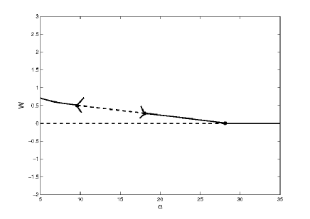
Figure 6: bifurcation diagram of equilibrium $W^{\ast}$ as $\alpha$ varies. The dotted line corresponds to periodic solutions.

10 Conclusions

The epidemic model studied here differs from the classical ones for the population size, which is not constant. As pointed out in [12], this leads to the possibility of having multiple endemic equilibria. In our case, which is regulated by a very different mechanism, we are able to show that under some conditions two endemic equilibria occur. One of them is unstable and the other is stable.

It is well known that, when the population size is fixed and transmission is inter-cohort, one has uniqueness of endemic states. See for example [4] and [9]. The stability of the steady states is studied in [18], [7] and we obtain here an analogous stability change for the trivial equilibrium.

For the sake of simplicity we have limited ourselves to investigating the case of inter-cohort transmission. Allowing for a general transmission kernel $\lambda(a,t)=\int_{0}^{a^{\dagger}}K(a,\sigma)I(\sigma,t)\,d\sigma$ makes the analysis of the model very difficult already in the case of constant population size (see [14]), while we wished to emphasise the peculiarities due to infection-related deaths.

The situation where multiple endemic equilibria exist may not be realistic. In fact, the model studied assumes that contagion can happen only in the first and in the last period of an individual life. A somehow similar situation was studied in [5], where the infection rate is piecewise constant. More precisely, juveniles and noncore adults cannot be infected, while only core adults can.

We have shown that the model with age-structured contact rates and variable population, because of infection-related deaths, has a much richer bifurcation diagram than models with only one of these features. For example, if (8.1), (8.2) and (8.4) hold, there is a change of stability and the presence of the extra-mortality destabilises the endemic equilibrium. Moreover, if either (9.2) or (9.3) holds, Hopf bifurcations occur.

We believe to have shown the main theoretical steps necessary to determine the stationary solutions of the model and their stability properties, adding the use of the numerical tool provided in [3] whenever analytical conclusions are hard, when not impossible, to draw. We also have highlighted the complexity of this model, that presents different kinds of dynamics.

References

[1]R.M. Anderson, R.M. May,Population biology
of infectious diseases: Part I, Nature 280 (1979), 361–367.
[2]V. Andreasen,Disease regulation of
age-structured host populations, Theoret. Population Biol. 36
(1989), no. 2, 214–239.
[3]D. Breda, M. Iannelli, S. Maset, R. Vermiglio,Stability analysis of the Gurtin-MacCamy model, SIAM J. Numer.
Anal., 46 (2008), no. 2, 980–995.
[4]S. Busenberg, K. Cooke, M. Iannelli,Endemic thresholds and stability in a class of age-structured
epidemics, SIAM J. Appl. Math. 48 (1988), no. 6, 1379–1395.
[5]S. Busenberg, K. Cooke, H. Thieme,Demographic change and persistence of HIV/AIDS in a
heterogeneous population, SIAM J. Appl. Math. 51 (1991),
no. 4, 1030–1052.
[6]Y. Cha, M. Iannelli, F.A. Milner,Existence
and uniqueness of endemic states for the age-structured S-I-R
epidemic model, Math. Biosci. 150 (1998), no. 2, 177–190.
[7]Y. Cha, M. Iannelli, F.A. Milner,Stability change of an epidemic model, Dynam. Systems Appl.
9 (2000), no. 3, 361–376.
[8]O. Diekmann, J.A.P. Heesterbeek,Mathematical
epidemiology of infectious diseases. Model building, analysis and
interpretation, Wiley Series in Mathematical and Computational Biology,
John Wiley & Sons, Ltd., Chichester 2000.
[9]D. Greenhalgh,Threshold and
stability results for an epidemic model with an age-structured meeting
rate, IMA J. Math. Appl. Med. Biol. 5 (1988), no. 2, 81–100.
[10]M.E. Gurtin, R.C. MacCamy,Non-linear
age-dependent population dynamics, Archiv. Rat. Mech. Anal.
54 (1974), no. 3, 281–300.
[11]K.P. Hadeler, K. Dietz,Nonlinear
hyperbolic partial differential equations for the dynamics of
parasite populations, Comput. Math. Appl. 9 (1983), no. 3,
415–430.
[12]W.Z. Huang, K.L. Cooke, C. Castillo-Chavez,Stability and bifurcation for a multiple-group model for the
dynamics of HIV/AIDS transmission, SIAM J. Appl. Math. 52
(1992), no. 3, 835–854.
[13]M. Iannelli,Mathematical theory of
age-structured population dynamics, Applied Mathematics Monograph
C.N.R. 7, Giardini Ed., Pisa 1995.
[14]H. Inaba,Threshold and stability results
for an age-structured epidemic model, J. Math. Biol. 28
(1990), no. 4, 411–434.
[15]J. Li, Z. Ma, Y. Zhou,Global
analysis of SIS epidemic model with a simple vaccination and
multiple endemic equilibria, Acta Math. Sci. Ser. B Engl. Ed.
26 (2006), no. 1, 83–93.
[16]R.M. May,Population biology of
microparasitic infections, in: Mathematical ecology, Eds.:
T.G. Hallam and S.A. Levin, 405–442, Biomathematics 17,
Springer, Berlin 1986.
[17]I. Mazzer,Un modello per la
dinamica di più popolazioni: esistenza, unicità e
approssimazione numerica della soluzione, tesi di Laurea
Specialistica in Matematica, University of Udine, supervisor
R. Vermiglio, Udine, 14 October 2009.
[18]H.R. Thieme,Stability change of the
endemic equilibrium in age-structured models for the spread of
S–I–R type infectious diseases, Differential equations models in
biology, epidemiology and ecology (Claremont, CA, 1990), 139–158,
Lecture Notes in Biomath. 92, Springer, Berlin 1991.