Automated supervised classification of variable stars.

Abstract

Context. Scientific exploitation of large variability databases can only be fully optimized if these archives contain, besides the actual observations, annotations about the variability class of the objects they contain. Supervised classification of observations produces these tags, and makes it possible to generate refined candidate lists and catalogues suitable for further investigation.

Aims. We aim to extend and test the classifiers presented in a previous work against an independent dataset. We complement the assessment of the validity of the classifiers by applying them to the set of OGLE light curves treated as variable objects of unknown class. The results are compared to published classification results based on the so-called extractor methods.

Methods. Two complementary analyses are carried out in parallel. In both cases, the original time series of OGLE observations of the Galactic bulge and Magellanic Clouds are processed in order to identify and characterize the frequency components. In the first approach, the classifiers are applied to the data and the results analyzed in terms of systematic errors and differences between the definition samples in the training set and in the extractor rules. In the second approach, the original classifiers are extended with colour information and, again, applied to OGLE light curves.

Results. We have constructed a classification system that can process huge amounts of time series in negligible time and provide reliable samples of the main variability classes. We have evaluated its strengths and weaknesses and provide potential users of the classifier with a detailed description of its characteristics to aid in the interpretation of classification results. Finally, we apply the classifiers to obtain object samples of classes not previously studied in the OGLE database and analyse the results. We pay specific attention to the B-stars in the samples, as their pulsations are strongly dependent on metallicity.

1 Introduction

In the last decade, astronomy witnessed several major advances. The advent of large detection arrays, the operation of robotic telescopes and the consolidation of high duty cycle space missions have provided astronomers with a wealth of observations with unprecedented sensitivity in virtually the whole electromagnetic spectrum during long uninterrupted periods of time. At the same time, the ever-growing storage capacity of digital devices has made it possible to archive and make these enormous datasets available. The consolidation of the Virtual Observatory (VO) technology and the interoperability provided by its services make it possible for the astronomer to work consistently on large portions of the electromagnetic spectrum, combining different data models (magnitudes, colours, spectra, radial velocities, etc).

The traditional procedures for data reduction and analysis do not scale with the sizes of the available data warehouses. Some of its components have been automated and can now be carried out in a systematic way, but it is becoming evident that optimal scientific exploitation of these databases requires the addition of information inferred from the observed data to enable the extraction of homogeneous (in some sense) samples of observations for further specific studies that could not be applied to the entire database. The process by which this added value is extracted is widely known as Knowledge Discovery and relies mostly on recent advances in the artificial intelligence fields of pattern recognition, statistical learning or multi-agent systems.

The use of these new techniques has the particular advantage that, once accepted that every search for a given type of object is biased ab initio by the adopted definition of that class, automatic classifiers produce consistent object lists according to the same objective and stable criteria openly declared in the so-called training set. We thus eliminate subjective and unquantifiable considerations inherent to, for example, visual inspection and produce object samples comparable across different surveys.

Altogether, the integration of Computer Science techniques (Grid computing, Artificial Intelligence and VO technology) and domain knowledge (physics in this case), and the new possibilities that this synergy offers are known as e-Science. Science proceeds in much the same way as before; the e- prefix only provides the basis to approach more ambitious scientific challenges, feasible on the grounds of more and better quality data.

In Debosscher et al. (2007, hereafter paper I) we introduced the problem of the scientific analysis of variable objects and proposed several methods to classify new objects on the basis of their photometric time series. The OGLE database (see section 2 for a summary of its objectives and characteristics) exemplifies some of the difficulties described in previous paragraphs. Although not its principal target, the OGLE survey has produced as a by-product hundreds of thousands of light curves of objects in the Galactic bulge and in the Large and Small Magellanic Clouds. These light curves have been analysed using the so-called extractor methods. Extractor methods can be assimilated to the classical rule-based systems where the target objects are identified by defining characteristic attribute ranges (where attribute is to be interpreted as any of the parameters used to describe the object light curves such as the significant frequencies, harmonic amplitudes or phase differences) where these objects must lie. In a subsequent stage, individual light curves are visually inspected and the object samples refined on a per object basis.

In this work we also present an extension of the classifiers defined in Paper I, to handle photometric colours. In section 2 we summarize the objectives and characteristics of the OGLE survey; section 3 describes the sources and criteria used for the assignment of colours to the training set and section 4 compares the results of the application of the classifiers (both with and without colours) to the OGLE database (bulge and Magellanic Clouds) with object lists available in the literature (obtained by means of extractor methods and human intervention) for a reduced set of classes. Finally, we analyse the object lists obtained with our classifiers for special classes in the realm of multiperiodic variables, not previously studied in an extensive way (to the best of our knowledge) in the context of the OGLE database.

2 The OGLE database and its published Catalogues of variables.

The Optical Gravitational Lensing Experiment (OGLE) is a long term joint microlensing survey aimed at detecting the Galaxy dark matter halo by its bending effect on the light coming from background stars. As a by-product, the project has been generating light curves of millions of stars of varying signal-to-noise ratiosx. The project has undergone several major upgrades. The data treated here belong to the OGLE-II phase of the project.

The OGLE database at the time of writing contains time series of several hundred thousand variable objects, all of which have been analysed by us, using the codes and techniques presented in Paper I. The bulge, LMC and SMC OGLE catalogues have been searched for particular variability types in the past (see Table 1) using extractor methods. In the following sections we briefly describe, where possible, the extraction rules used in the construction of each of the catalogues in order to provide a proper framework for the analysis of the classification results and to facilitate the explanation of possible discrepancies.

Table 1: Published catalogues used in comparison with the outcome of our classifiers.

Variability class	Source object	Reference	Number of objects
RR Lyrae	LMC	Soszynski et al. (2003)	5455 (RRab) ; 1655 (RRc) ; 272 (RRe) ; 230 (RRd)
RR Lyrae	SMC	Soszynski et al. (2002)	458 (RRab) ; 56 (RRc) ; 57 (RRd)
Cepheids	LMC	Udalski et al. (1999b)	1335
Cepheids	SMC	Udalski et al. (1999c)	2049
Double mode Cepheids	LMC	Soszynski et al. (2000)	81
Double mode Cepheids	SMC	Udalski et al. (1999a)	95
Pop. II Cepheids	LMC	Kubiak & Udalski (2003)	14
Pop. II Cepheids	bulge	Kubiak & Udalski (2003)	54
Eclipsing binaries	LMC	Wyrzykowski et al. (2003)	2580
Eclipsing binaries	SMC	Wyrzykowski et al. (2004)	1350
Eclipsing binaries	LMC	Groenewegen (2005)	178
Eclipsing binaries	SMC	Groenewegen (2005)	16
Eclipsing binaries	Bulge	Groenewegen (2005)	2053
Long period Variables	LMC	Soszynski et al. (2005)	3221
Mira	Bulge	Matsunaga et al. (2005)	1968
Mira	Bulge	Groenewegen & Blommaert (2005)	2691
Various	Bulge	Mizerski & Bejger (2002)	4597
$\delta$-Scuti	Bulge	Pigulski et al. (2006)	193

In Table 1 we include information on the number of objects in each of the published catalogues. These numbers include double detections in overlapping zones across different fields. We include these double detections because they are represented by independent light curves, and we are mainly interested in the true/false positive/negative detection rates, not so much in the objects lists themselves (except in the analysis of multiperiodic variables).

The classifiers presented in Paper I and the colour extensions presented here and discussed below were applied to the OGLE LMC/SMC (Zebrun et al. 2001) and Galactic Bulge (Wozniak et al. 2002) catalogues as downloaded from http://bulge.astro.princeton.edu/$\sim$ogle/ogle2/dia/ and ftp://bulge.princeton.edu/$\sim$ogle/ogle2/bulge_dia_variables respectively. Again, these catalogues contain duplicate entries that we kept for the same reasons as above. According to Eyer (2002) and Eyer & Woźniak (2001), the catalogues include spurious detections of variable objects. In Eyer (2002), these spurious detections are discussed and several systematic effects identified (chip perturbations, mirror realuminization and proximity to bright objects). In Eyer & Woźniak (2001), the authors discover a type of artifact introduced by the difference image analyses (DIA) consisting of the occurrence of pairs of monotonic anti-correlated light curves as a result of the presence of high proper motion stars in dense fields. The impact of these artifacts is restricted to the Bulge fields and, since i) they do not result in periodic signals and ii) systematic trends are removed from the fits to the data (see Paper I), we do not expect them to affect our results significantly.

The detailed study of the first type of artifacts is out of the scope of this work. Nevertheless, it would be extremely interesting to investigate how these artifacts are classified by our algorithms and, most importantly, the possibility of detecting them as a separate group by using clustering techniques. This is presently being studied as part of the Gaia effort to ensure a robust data processing pipeline.
In the five following subsections we discuss the work in the literature already done from the OGLE light curves. We regard these “human” classification results as correct and compare our automated results with them to evaluate the latter.

2.1 RR Lyrae variables

The selection of the RR Lyrae variables in the OGLE catalogues was made in several stages (see Soszynski et al., 2002 for the SMC and Soszynski et al., 2003 for the LMC). In the first stage, variable stars were identified on the basis of the standard deviation of all individual OGLE PSF measurements. Their light curves were analysed using the Analysis of Variance (AoV) algorithm and all objects showing statistically significant periodic signals were then visually inspected and manually classified into one of several classes. In the second stage, DIA photometry was used to select candidates with I magnitudes between 15 and 20 for the LMC (18.4 and 19.4 for the SMC), and with standard deviations at least 0.01 mag above the median value of the standard deviations of stars of equal brightness for the LMC (0.02 for the SMC in the I band and 0.05 for the V band). Again, periodic signals were searched for, and stars with periods longer than 1 day and/or signal-to-noise ratios below 3.5 were rejected. Then, Fourier analysis was performed and unspecified rules were applied to extract each of the RR Lyrae subtypes. Single mode pulsators were selected according to their position in the $\log P$-$R_{21}$($=\frac{A_{12}}{A_{11}}$) and $\log P$-$amplitude$ diagrams, where $R_{21}=\frac{A_{12}}{A_{11}}$ is the amplitude ratio of the first two harmonics of the first significant frequency. The separation of first overtone pulsators is based on a threshold of $P>0.26$ d. Second overtone pulsators were selected amongst stars with periods below 0.3 days as those with low amplitude sinusoidal light curves, which involves again visual inspection of the light curves one by one. Finally, double mode pulsators were sought by selecting those stars with statistically significant second frequencies at a ratio close to $0.745$ of the first one. Again, all light curves and power spectra were carefully inspected before they were included in the double mode RR Lyrae stars catalogue.

Bulge RR Lyrae variables in Sumi (2004) were selected by fitting an ellipse to the locus of stars in a diagram representing the ratio of the second to first harmonic amplitude ($R_{21}$) and the phase difference between these harmonics ($\phi_{21}$ or $PH_{12}$ in Paper I; see e.g. Fig. 5), and using a hard threshold decision boundary, according to the method first proposed by Alard (1996). The ellipse is centered on (4.5 rad, 0.43) with semi-major axis $a=0.8$ and semi-minor axis $b=0.17$, and the angle between the horizontal and the major axis is $-10\deg$. These candidates have been further refined and analysed in a recent study by Collinge et al. (2006).

2.2 Cepheids

The catalogues of Cepheid variables in the OGLE database have been presented in Kubiak & Udalski (2003), Udalski et al. (1999b) and Udalski et al. (1999c). In the identification of Cepheids, objects with I magnitudes brighter that 19.5 (LMC) and 20 (SMC) were selected for further analysis based on the visual inspection of the light curves and their position in the colour-magnitude diagram (CMD). The region occupied by Cepheid pulsators has been defined by the authors to be upper bounded by $I<18.5$ and delimited in colour by $0.25<V-I<1.3$. Objects with no available colours or colours to the right of the red boundary were recovered if their light curves were conspicuously of the Cepheid type. Again, visual inspection of all light curves was a main ingredient of the classification process.

Double mode Cepheids were identified amongst Cepheids by fixing the range of allowed frequency ratios to $0.735\pm 0.02$ (first overtone to fundamental mode) or $0.805\pm 0.02$ (second to first overtone) in the case of the prewhitened search for second periods from Fourier Analysis, and the same ratios $\pm 0.015$ for the application of the CLEAN algorithm (Roberts et al. 1987). See Udalski et al. (1999a) and Soszynski et al. (2000) for the SMC and LMC catalogues respectively.

The catalogue of Population II Cepheids in the bulge has been presented in Kubiak & Udalski (2003). It is defined in the period range between 0.6 and a few days and, again, the selection was based on the visual inspection of the light curve shapes and their similarities to those described by Diethelm (1983).

2.3 Eclipsing binaries

Eclipsing binaries in the Large and Small Magellanic Clouds have been extracted using different methods. While the SMC eclipsing binaries were identified on the basis of visual inspection of the folded light curves of all variable objects (Wyrzykowski et al. 2004), LMC eclipsing binaries were preselected by a neural network (Wyrzykowski et al. 2003). An artificial neural network was trained on two dimensional images of folded light curves of the first field (LMC_SC1), selected to separate unseen light curves into three main types: eclipsing, sinusoidal and saw-shape. The training proceeded until the mean training error was below $10^{-8}$. Then, the refinement and subclassification of the eclipsing candidates was carried out by visual inspection of the folded light curves.

Groenewegen (2005) has constructed a catalogue of candidate eclipsing binary systems in the Galactic bulge suitable for distance estimation (mainly detached systems), based on the statistical properties of the phased light curve and subsequent visual inspection. Furthermore, Mizerski & Bejger (2002) have provided a list of candidate W UMa systems based on typical values of the Fourier coefficients of their light curve decompositions calculated by Rucinski (1993).

2.4 Long period variables

Catalogues of Mira and semiregular Variables in the LMC have been presented in Soszynski et al. (2004, 2005). The frequency analysis was similar to the one described for all previous variability types and the selection criteria were based on the I band magnitude ($I<17$) and on the position in the period–NIR Wessenheit index diagram. In this diagram, sequences C and C’ (see Wood et al., 1999) were identified as Miras and semiregular Variables. Furthermore, stars in the B sequence can also be assigned to the Mira-semiregular category if the secondary period falls in any sequence except sequence A. No quantitative criterion was given to separate sequences in the plot, so the assignment of a star to any of the sequences is subjective.

Recently, Groenewegen & Blommaert (2005) and Matsunaga et al. (2005) have published catalogues of Mira variables in the Galactic bulge. The selection criterion in the first case was simply based on $I$-band light curve amplitudes (in the sense of peak-to-peak range) above 0.9 mag followed by visual inspection, and resulted in a sample of 2691 objects. In the second catalogue, the selection criteria were periods above 100 days, amplitudes larger than 1.0 in the $V$ magnitude and $\theta$ values (the phase dispersion minimization regularity indicator) below 0.6, followed by visual inspection. This resulted in a sample of 1968 Mira variables in the OGLE bulge fields.

2.5 Delta Scuti stars in the Galactic bulge.

Mizerski & Bejger (2002) and Pigulski et al. (2006) have published lists of high amplitude $\delta$ Scuti (HADS) stars in the bulge fields. In the first case (only the first bulge field), no criterion was given for the selection of the 11 HADS candidates but reference is made to the use of luminosities in the identification process. In the second work, a HADS star was defined as a star with a period less than 0.25 days for which at least one harmonic of the main mode was detected and which was not an RR Lyrae star or W UMa system (distinguished by means of the Fourier coefficients and visual inspection of the light curve).

3 The extended classifier: using colour information

All objects in the bulge, LMC and SMC OGLE catalogues were subject to the frequency analysis described in Paper I. The final numbers of objects analysed with this method are 50708 in the LMC, 14473 in the SMC and 214786 in the Galactic bulge.

In an effort to improve the performance of the classifiers presented in Paper I, we have constructed alternative ones with colour information added to the basic time series parameters described therein. This is not a mere upgrade making the previous release obsolete since many archives provide no colour information for classification. This is the case, for example, for the Optical Monitoring Camera onboard INTEGRAL, that has returned thousands of light curves, only a small fraction of which have diachronic colours available.

The process to incorporate photometric colours in the classifiers followed the same scheme described in Paper I for the time series classifiers. For the training set presented there, a search was conducted in the Hipparcos catalogue (Perryman & ESA 1997) and SIMBAD in order to retrieve magnitudes in the Johnson photometric system. Johnson’s colours for training set objects from the OGLE database (double mode pulsators and eclipsing binaries) were preferentially retrieved from the catalogues by Wyrzykowski et al. (2003), Soszynski et al. (2000), and Soszynski et al. (2002). Additionally, the 2MASS catalogue of Cutri et al. (2003) was searched for counterparts in order to add the $J-H$ and $H-K$ colour attributes to the original training set. The search was conducted imposing a 3 arcsec search radius and quality flags A and/or B in the three bands.

Synchronicity between the observations in the different passbands cannot be assured when only SIMBAD colours were available. This is especially relevant for the case of large amplitude variables where observations in opposite phases of the light curve can lead to totally erroneous colour indices. Fortunately, the vast majority of training examples of large amplitude classes are taken either from the HIPPARCOS/Tycho catalogue or from the OGLE database itself, thus minimizing the impact of diachronic observations in our training set.

The inclusion of colour information was done separately for several colour sets. In order to assess the relevance of the infrared colours for the classification task, two versions of the training set (with and without 2MASS colours) were constructed. Additionally, two versions of each training set (with and without the $B-V$ colour) were created. The reason for this is the fact that we were not able to obtain $B-V$ colours for a large fraction of the OGLE bulge variables. Therefore, the assessment of the classifier results conducted on bulge variables (see below) only incorporates the $V-I$ and 2MASS colours.

As a result, $B-V$, $V-I$, $J-H$ and $H-K$ colours were obtained for at least 77% of the stars in the training set (1344 of 1754 instances). The exact sizes of each training set are as follows:

1. $V-I$ : 1602 instances

2. $B-V$ and $V-I$: 1592 instances

3. $V-I$, $J-H$ and $H-K$: 1348 instances

4. $B-V$, $V-I$, $J-H$ and $H-K$: 1344 instances

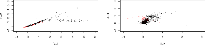
Figure 1: Training set colours. Black dots indicate training set objects in the Galaxy whereas red circles correspond to the classes defined with OGLE members, i.e. eclipsing binaries and double mode Cepheids and RR Lyrae stars.

Figure 1 shows two colour-colour diagrams for Johnson and 2MASS photometry of the training set.

Strömgren colours were also searched in the catalogue by Hauck & Mermilliod (1998). Unfortunately, they were only found to be available for a much smaller fraction (less than 50%) of the training set and covering only certain variability classes, leaving the less frequent ones almost unrepresented. A complete classifier with ability to predict classes using Strömgren colours has been developed only for multiperiodic variables, where the impact of such information was found to be optimal, but will not be the subject of analysis in the following.

Colours for the OGLE Galactic bulge, LMC and SMC objects used for testing were obtained from the 2MASS and OGLE databases. 2MASS objects within a search radius of 3 arcseconds and quality flags A or B were assumed to be counterparts of the OGLE objects. With these parameters, we retrieve 43351 instances (objects) with Johnson colours ($B-V$ and $V-I$) amongst the 50708 LMC objects (see section 2), and 26720 with combined Johnson and 2MASS colours; 12425 SMC objects with Johnson colours and 6937 with Johnson and 2MASS colours; and 146034 bulge objects with $V-I$ (all of which have 2MASS photometry too). The fraction of bulge objects with $B-V$ colours available was so small that we preferred to work with $V-I$ and 2MASS photometry alone.

We have found a systematic difference in the $J-H$ colours of eclipsing binaries in the Hipparcos sample and in the OGLE LMC catalogue. Figure 2 shows two colour-colour diagrams of Hipparcos and OGLE LMC eclipsing binaries in Johnson and 2MASS photometric bands respectively.

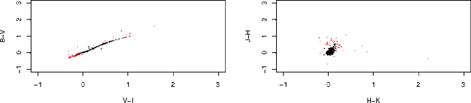
Figure 2: Colour-colour diagrams of the eclipsing binaries in the Hipparcos (black dots) and OGLE (red circles) catalogues.

Visual inspection of the plots reveals what seems a selection effect in the choice of eclipsing binaries for the training set. The reason for choosing OGLE eclipsing systems (all from the LMC) is their very good sampling quality. It seems that favouring high signal-to-noise ratios has biased the sample towards blue objects with an unexplained excess in the $J-H$ colour. We have not found a plausible explanation for the concurrence of both effects but we expect to improve the eclipsing binaries prototypes in the training set with new examples from the CoRoT database.

All objects from the OGLE database (either in the training set or in the test set) have been dereddened using OGLE extinction maps: Udalski et al. (1999b) for the LMC and Udalski et al. (1999c) for the SMC. Objects in the Galactic bulge were dereddened using the extinction maps by Sumi (2004). The extiction values of OGLE field number 44 (missing in the original work due to the lack of red clump giants well above the V band detection limit) are approximated by the corresponding values in the closest OGLE field (number 5). All extinction maps were combined with the classical CCM extinction curve by Cardelli et al. (1989). For bulge variables this extinction curve produces corrections indistinguishable from those of Draine (2003) used by Groenewegen & Blommaert (2005) in their analysis of Mira variables. Gordon et al. (2003) have studied the validity of the classical CCM relationship for the Magellanic Clouds. Figures 2–6 in their work seem to suggest that the CCM curve is a safe approximation (to within the measurement errors) of the Magellanic Clouds extinction curves in the infrared bands considered here.

Unfortunately, the reddening correction applied to the colour indices and described above will only produce strictly valid results for stars at the mean distance of the red clump giants used in the derivation of the extinction maps.Our correction may be less accurate for other stars, but we do not have a better one available at present.

4 Classification results

In the following, we will refer to the sets of objects classified in one of the categories described in section 2 as class samples (e.g., the RR Lyrae sample or the Cepheids sample). In this section we will compare the results obtained by the automatic classifiers with those found in the literature. We have applied the battery of classifiers presented in Paper I and their extensions to treat colour information, to the OGLE LMC/SMC (Zebrun et al. 2001) and bulge (Wozniak et al. 2002) variability archives. Full results of the comparison of the statistical performance of the different classifiers will be published in a specialized journal. Here we only report on the overall best performing algorithm, the multi-stage classifier based on Bayesian Networks (MSBN) as well as on the Gaussian Mixtures classifier (GM), which was described in Paper I. The latter is simpler in its design and interpretation and works better than the former for the low-amplitude multiperiodic pulsator classes SPB and $\gamma$-Doradus. It is thus best suited to retrieve these types of asteroseismological targets (e.g. Cunha et al. (2007) for a review). The MSBN classifier on the other hand works better for the larger-amplitude monoperiodic variables (including eclipsing binaries), and for the other types of multiperiodic variables such as BCEP or DSCUT stars.

The multi-stage classifier based on Bayesian Networks (MSBN) takes advantage of several feature selection steps adapted to each classification problem. Trying to select a global feature set for the classification of the entire set of 35 classes results in a suboptimal trade-off because attributes crucial for the separation of two classes close to each other in the parameter space can be irrelevant in identifying the remaining 33. On the contrary, dividing the classification problem in several stages where smaller problems are tackled allows for the particularized selection of feature sets that are optimal in each step.

Several alternative groupings and orderings were attempted and different algorithms tried in each step and the resulting performances were either equal to or poorer using standard hypothesis testing procedures. Although the search could never have been exhaustive, the most reasonable combinations of groups of classes, orderings and attribute selection techniques have been explored, the one presented here resulting in the best overall performance. The classification algorithms tried include neural networks, Bayesian networks, support vector machines and Bayesian ensembles of neural networks; feature selection techniques include the wrapper approach for those algorithms where computation time made it feasible, and attribute set scores based on correlation, mutual information and symmetrical uncertainty between attributes and the class.

The MSBN has four stages of dichotomic classifiers, one for each of the main categories of classical variables: stage 1 to separate eclipsing from non-eclipsing variables; stage 2 to separate Cepheids and non-Cepheids; stage 3 to separate the long period variables from the rest, and stage 4 to separate RR Lyrae variables from the rest (stage 6 is also dichotomic, but corresponds to a more specialized level that separates long period variables into the Mira and Semiregular types). It starts with a first dichotomic classifier that attempts to separate eclipsing binaries from all other variability types. The attribute set used in the first and subsequent stages is listed in Table 3. The second dichotomic stage separates the group of classes CLCEP, PTCEP, RVTAU and DMCEP (see Table 2, an abridged version of Table 2 in Paper I, for class abbreviations) from all other classes. Then, a third classifier attempts to identify the group of long period variables (MIRA and SR) and a fourth classifier separates RR Lyrae stars (RRAB, RRC and RRD) from the rest of the classes. Complementary to these, there are specialized classifiers that separate classes within groups. There is a classifier for Cepheids that classifies CLCEP, PTCEP, RVTAU and DMCEP, and equivalent classifiers for long period variables and RR Lyrae stars. The subclassification of eclipsing binaries is made according to the methodology described in Sarro et al. (2006). Finally, there is a classifier that separates all other classes not included in the groupings described above, i.e. irregular and most multiperiodic variables. The complete class probability vector for an object is computed combining the output from all classifiers. For example, the probability of belonging to class RRC is the probability of not being an eclipsing binary (stage 1) times the probability of not being a Cepheid (stage 2) times the probability of not being a long period variable (stage 3) times the probability of being an RR Lyrae pulsator (stage 4) times the probability of being an RRC pulsating star (stage 7).

Class	Abbreviation
Periodically variable supergiants	PVSG
Pulsating Be-stars	BE
$\beta$-Cephei stars	BCEP
Classical Cepheids	CLCEP
Beat (double-mode)-Cepheids	DMCEP
Population II Cepheids	PTCEP
Chemically peculiar stars	CP
$\delta$-Scuti stars	DSCUT
$\lambda$-Bootis stars	LBOO
SX-Phe stars	SXPHE
$\gamma$-Doradus stars	GDOR
Luminous Blue Variables	LBV
Mira stars	MIRA
Semi-Regular stars	SR
RR-Lyrae, type RRab	RRAB
RR-Lyrae, type RRc	RRC
RR-Lyrae, type RRd	RRD
RV-Tauri stars	RVTAU
Slowly-pulsating B stars	SPB
Solar-like oscillations in red giants	SLR
Pulsating subdwarf B stars	SDBV
Pulsating DA white dwarfs	DAV
Pulsating DB white dwarfs	DBV
GW-Virginis stars	GWVIR
Rapidly oscillating Ap stars	ROAP
T-Tauri stars	TTAU
Herbig-Ae/Be stars	HAEBE
FU-Ori stars	FUORI
Wolf-Rayet stars	WR
X-Ray binaries	XB
Cataclysmic variables	CV
Eclipsing binary, type EA	EA
Eclipsing binary, type EB	EB
Eclipsing binary, type EW	EW
Ellipsoidal binaries	ELL

Table 2: Stellar variability classes and the code abbreviation used in Paper I.

Table 3: Attributes used in each classification stage by the sequential classifier. Abbreviations used are as follows: log-fi represents the logarithm of the i-th frequency; log-fi-fj is the logarithm of the ratio fi/fj; afi represents the sum of squares of the harmonic amplitudes in frequency i; log-afihj-t is the logarithm of the total amplitude of the j-th harmonic of the i-th frequency; log-crfij is the logarithm of the jth ratio of harmonic amplitudes of the i-th frequency (j=0 corresponds to the ratio of the amplitude of the second harmonic over that of the first, j=1, to the ratio of the amplitude of the third harmonic over that of the first and so on); log-crfihj-fi’hj’ represents the logarithm of the amplitude ratio between harmonics j and j’ of frequencies i and i’ respectively; pdfij is the j-th phase difference between the various harmonics of the i-th frequency (j=0 corresponds to the first and second harmonics, j=1, to the third and first harmonics, and so on); varrat represents the variance ratio defined in Paper I.

Stage	Classes & Attributes
1	Eclipsing/non eclipsing
	log-f3, log-f2-f1, log-af1h1-t, log-crf10, log-crf15, log-crf20, log-crf25, log-crf32, log-crf33, pdf12, pdf13, pdf14, pdf23
2	Cepheids/non Cepheids
	log-f1, log-f2-f1, af1, af2, log-af1h1-t, log-af1h2-t, log-crf3h1-f1h1, log-crf10, log-crf11, log-crf14, pdf12, varrat
3	Red giants/non red giants
	log-f1, log-f2, log-f3, log-f2-f1, af1, af2, log-af1h1-t, log-af2h3-t, log-crf21, log-crf24, log-crf30
4	RR Lyrae/Non RR Lyrae
	log-f1, af1, log-af1h1-t, log-af3h1-t, log-crf3h1-f1h1, log-crf11, log-crf14, pdf12, pdf13
5	CLCEP/DMCEP/PTCEP/RVTAU
	log-f1, log-af1h1-t, log-af2h3-t, log-af2h4-t, log-af3h4-t, log-crf12, log-crf32, pdf12, varrat
6	MIRA/SR
	af1, log-af1h1-t, log-af1h3-t, log-af2h4-t, log-af3h3-t, varrat
7	RRAB/RRC/RRD
	log-f1, log-f2-f1, af1, log-af1h2-t, log-crf2h1-f1h1, log-crf10, pdf12, varrat
8	PVSG BE BCEP CP DSCUT ELL GDOR HAEBE HMXB LBOO LBV PTCEP ROAP SPB SXPHE TTAU WR FUORI PSDB
	log-f1, log-af2h1-t, log-crf2h1-f1h1, log-crf10, log-crf13

In the next sections, the classifiers are applied to the entire list of objects flagged by the OGLE team as variable. Also, they are applied to the object samples referenced in section 2. Again, it has to be born in mind that not all objects in the samples have been identified by the algorithms described in Paper I as having at least a significant frequency and therefore, the column named ’Total number of objects’ in the following tables always refers to this set of objects fulfilling the two criteria: being identified in the literature as belonging to a variability class and with a positive frequency identification.

In general, the three populations observed by OGLE (the Galactic bulge and the Large and Small Magellanic Clouds) are very different from a statistical point of view. In this work we have found it clearer to illustrate the performance of the classifiers with plots of the LMC samples since they represent a compromise in the number of stars in each sample, both sufficient for statistical purposes and, at the same time, not so large that the plots become uninterpretable. Equivalent plots for the Galactic Bulge populations are included as online material (corresponding to the results presented by Mizerski & Bejger (2002) for the first bulge field) while SMC figures can be obtained upon request from the authors.

4.1 RR Lyrae stars

Table 4 summarizes results obtained with each of the classifiers (GM and MSBN) on OGLE data without colours added (NC), with $B-V$ and $V-I$ colours (+BVI) and with all colours (+JHK). The experiments in the bulge did not include $B-V$ for the reasons explained in section 3. The Gaussian Mixtures classifier only makes use of the $B-V$ colour index except in the bulge where only the $V-I$ colour index was used.

In the LMC, Soszynski et al. (2003) found 7612 RR Lyrae stars. A search was performed in the OGLE variability database using the coordinates provided by the authors in the electronic version of the catalogue. This search only produced photometric time series for 2734 (plus 56 double mode pulsators published in a separate catalogue). The situation is analogous to the SMC where Soszynski et al. (2002) list a total of 571 RR Lyrae stars but we are only able to identify corresponding entries in the variability database for 89 (plus 4 double mode pulsators that we will not include in the study since these systems are part of the training set). We have found no explanation for this large discrepancy and thus, in the following we compare our detection rate with these total numbers (2790 for the LMC and 89 for the SMC).

In the LMC, the multistage classifier based on Bayesian Networks correctly identifies as RR Lyrae 2597 of the 2790 stars (93%) classified as such by the OGLE team. The percentage increases to a 96% when BVI colours are used as attributes for classification. In the SMC, the percentage increases up to a 95.5% without colours and 98% with BVI colours. As could be expected, the low signal to noise ratios of the 2MASS detections worsens the percentages down to 85% in the LMC while the SMC detection rate is too low to draw significant conclusions. In the bulge, the same classifier has a performance of 87% working on time series attributes alone (NC) and much poorer performances when colours are added. We interpret this as the result of a poor dereddening using field average values of the extinction. Since the $V-I$ value was obtained from the OGLE project itself, we believe there is no room for the interpretation of this performance degradation as being produced by counterpart misidentifications.

The largest errors of the sequential classifier in these category of variable stars are RR Lyrae systems misclassified as double mode Cepheids or eclipsing binaries. This is interpreted as the effect of overfitting to the training set, that is, as a consequence of the fact that DMCEP (see Table 2 for abbreviations) and eclipsing binaries are the only classes, together with double mode RR Lyrae stars, whose training examples are taken from the OGLE database. In this sense, the classifier is recognizing similarities likely due to the observational setup of the OGLE survey and common to the three classes whose prototypes are taken from its database. The GM classifier is clearly more robust against overfitting as shown in the table and in the section devoted to the analysis of Cepheid stars.

Table 4: Number of RR Lyrae stars according to the OGLE catalogues and correctly identified by the Gaussian Mixtures (GM) and multistage Bayesian networks (MSBN) classifiers presented here. The table lists the number of stars in the OGLE catalogues with a clear counterpart in the OGLE variability database and, subsequently, the fraction of these with available visible and visible+2MASS colours.

Catalogue	Source	Potential detections			GM		MSBN
		NC	+(B)VI	+JHK	NC	+(B)VI	NC	+(B)VI	+JHK
OGLE RR Lyrae	LMC	2790	2558	137	2014	1819	2597	2457	117
OGLE RR Lyrae	SMC	93	87	2	63	61	89	85	2
OGLE RR Lyrae	bulge	70	22	17	61	7	61	12	6

The RR Lyrae sample compiled by the OGLE team also provides subtype information. Therefore, we can further compare the subclassification of RR Lyrae stars into one of its subclasses: RRab, RRc and RRd. Table 5 summarizes the confusion matrix obtained with the sequential classifier based on Bayesian networks and with the GM classifier when applied to the LMC sample without colours.

Table 5: Confusion matrix for the RR Lyrae subtypes. Each column lists the number of objects of a given subtype (shown as column header) classified as all possible subtypes.

	GM			MSBN
	RRAB	RRC	RRD	RRAB	RRC	RRD
RRAB	1913	1	0	2420	4	2
RRC	0	22	0	3	76	0
RRD	1	21	54	21	14	53

Obviously, the True Positive Rate (TPR) is not the only way to measure the success of a classifier. The false positive rate (FPR, the number of non members of the class mistakenly classified as such) for a given class is also a good measure that quantifies the contamination degree of the resulting samples. Unfortunately, we can only measure the FPR coming from the OGLE sample classes other than RR Lyrae, described in section 2. However, we can find useful hints of the true FPR for example by looking at the definition plots of the RR Lyrae class. When applied to the whole of the LMC (SMC) database with 50708 (14473) instances, the sequential classifier finds 3019 (273) RRab candidates, 131 (18) RRc candidates and 335 (88) RRd candidates. We again attribute the large numbers of double mode pulsators to the use of OGLE examples of this class in the training set. Figures 3 and 4 show the position of the LMC candidates produced by the Bayesian and Gaussian Mixtures classifiers in the $\log(P)-R_{21}$ and $\log(P)-\phi_{21}$ diagrams.

The plots were constructed with all instances that fulfilled the condition that the class probability given the data ($p({\cal C}_{k}|{\cal D})$) was higher for RR Lyrae subtypes than for any other class. The plots can be adapted to a given decision threshold: setting $p({\cal C}_{k}=RR\leavevmode\nobreak\ Lyrae|{\cal D})>0.9$ in the sequential classifier, for example, removes most of the conspicuous ghost frequencies around $\log(P)=0,-0.3,-0.5$ (P in days) and most other stars not in the dense loci of the RR Lyrae subtypes. Similar thresholds can be defined for the GM classifier in terms of the Mahalanobis distance to the center of the cluster.

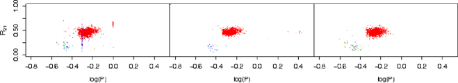
Figure 3: The $R_{21}-\log(P)$ plane of RRAB (red), RRC (green) and RRD stars (blue) in the LMC, according to the multistage Bayesian networks (left) and Gaussian Mixtures classifiers (middle) and the OGLE catalogue (right).

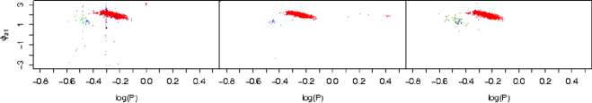
Figure 4: The $\phi_{21}-\log(P)$ plane of RRAB (red), RRC (green) and RRD stars (blue) in the LMC, according to the multistage Bayesian networks (left) and Gaussian Mixtures classifiers (middle) and the OGLE catalogue (right).

A comparison with the results by Collinge et al. (2006) is shown in Fig. 5. As summarized in section 2, they identify 1888 fundamental mode RR Lyrae candidates in the bulge plus 25 repetitions in overlapping regions between fields. The MSBN classifier finds 1862 (97%) candidates inside the ellipse that defines the RRab locus according to Sumi (2004). Besides these, the MSBN classifier provides 756 new candidates, not all inside the ellipse .

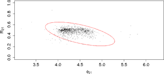
Figure 5: The $\phi_{21}-R_{21}$ plane of RRAB stars (90% decision threshold) in the bulge. The ellipse shows the decision boundary adopted by Sumi (2004) and Collinge et al. (2006).

One may wonder where the new RR Lyrae candidates are located in the parameter space. Since this space has a large number of dimensions, it will prove useful to project it onto planes as with previous plots. Figure 6 shows two such projections onto the $\log(P)$-$R_{21}$ and $\phi_{21}$-$R_{21}$ planes for stars in the LMC classified by the MSBN classifier as RR Lyrae, the latter plane being the one used by Collinge et al. (2006) to define the bulge sample of RR Lyrae stars. The first plot shows superimposed the contours of the probability density functions constructed using standard kernel methods applied to the RR Lyrae samples provided by the OGLE team. Both plots clearly show how the new candidates (with probabilities above 90%) fall mostly in the RR Lyrae locus. Although a detailed analysis of all new candidates in all the following categories is beyond the scope of this article, we have randomly checked some folded light curves of the new candidates such as those shown in Figure 7. Most of the new candidates have folded light curves similar to those in the left and upper right panels of the figure with varying signal-to-noise ratios. We show, completeness, the folded light curve of a star with a class assignment of RR Lyrae (with a low probability, though) and characterized by a low statistical significance of the frequency detection. It helps us exemplify why and how, imposing more stringent significance thresholds on the frequency detection, we can remove poor quality candidates from the lists.

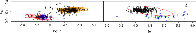
Figure 6: Two projections of three parameters (period, amplitude ratio and phase difference) of stars in the LMC classified as RR Lyrae and not in the OGLE RR Lyrae sample. In the left plot, contour lines represent the probability density as obtained from the OGLE sample by using kernel methods. Orange corresponds to the RRAB sample, red to RRC and blue to RRD. In the right plot, the ellipse is that used in Collinge et al. (2006).

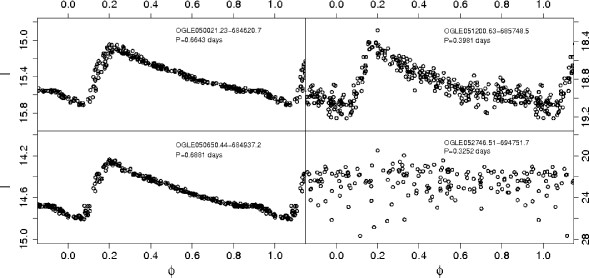
Figure 7: $I$-band light curves of three candidates of the RR Lyrae category not identified as such in the OGLE catalogue (longer period candidates in the upper and lower left plots and shorter period and lower signal-to-noise ratio in the upper right panel). The lower right plot is an example of a low probability candidate with no conspicuous modulation of the light curve.

4.2 Cepheids

Table 6 lists the results obtained for the LMC with the same classifiers tested in the previous section. In this case, the best performances (achieved by the MSBN classifier) in the LMC are of 94% without colours, 99% with BVI photometry and 98% with BVI plus JHK photometry. These performances are around 85% in the SMC although the use of 2MASS photometry increases the true positive rate back to 95%. In the bulge, the results confirm the problem with inadequate dereddening.

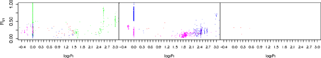
Figure 19: The $R_{21}-\log(P)$ plane of classical Cepheids (red), RVTAU (green), PTCEP (blue) and DMCEP (magenta) in the Galactic Bulge according to the multistage and GM classifiers and the OGLE team sample (only fundamental and first overtone classical Cepheids in red, and DMCEP in magenta).

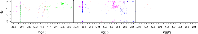
Figure 20: The $\phi_{21}-\log(P)$ plane of classical Cepheids (red), RVTAU (green), PTCEP (blue) and DMCEP (magenta) in the Galactic Bulge according to the multistage and GM classifiers and the OGLE team sample (only fundamental and first overtone classical Cepheids in red, and DMCEP in magenta).

While the OGLE Cepheids sample only contains and distinguishes fundamental and first overtone pulsators, our classifier identifies RVTAU and PTCEP systems. These are included in the plots describing the automatic classifiers but not in the OGLE sample plot (see Figures 8, 9, 19, and 20). It is evident from these plots that, as was indeed the case with the RR Lyrae systems, the MSBN classifier is overfitted to the training set and tends to overestimate the probability of the classes represented in the training set with examples taken from the OGLE database (double mode Cepheids in this case, double mode RR Lyrae pulsators in the previous one). This overfitting can also be detected in the analysis of the new DMCEP candidates according to the MSBN classifier, which are mostly first overtone classical Cepheids close in the hyperparameter space to the DMCEP locus, but lacking the characteristic frequency ratio. Apart from this effect (that can only be corrected when more examples of double mode pulsators from other surveys are available) we see that the MSBN classifier incorrectly assigns the DMCEP class to a cluster of RR Lyrae stars at $\log(P)\approx-0.2$ (P in days). This effect can be traced back to the density of DMCEP and RRAB training examples in that region, but it is evident that this classifier is not robust enough and requires a better sampling of the density of examples there. We have tried several modifications of the design presented in section 3 in order to redraw the boundary between double mode Cepheids and RR Lyrae stars. This seemingly simple task (both classes are linearly separable in several attributes according to the training set) turned out to result in undesired performance degradation (of the order of 15%) in the classical Cepheid detection (or true positive) rate. Solutions to this problem included new hierarchy designs (separating Cepheids and RR Lyrae systems at the same time), reordering of the partial classifiers and several different attribute selection techniques. In our opinion, the MSBN classifier described in section 3 represents a better global solution to the problem of automatic classification of variable objects that needs further refinement at the forementioned boundary. The GM classifier on the contrary, has no RR Lyrae contamination in the DMCEP candidate list despite being constructed upon the same training set.

Table 7 shows the confusion matrices for the subtypes of Cepheids common to the classifiers and OGLE catalogues. We see how the MSBN higher detection rate has, as an undesired side effect, a large number of misclassifications of classical Cepheids as double mode. Also, it is unable to correctly identify Population II Cepheids. Although there is also a sizable contamination of CLCEP stars in the DMCEP group produced by the GM classifier, the overfitting is less serious than in the MSBN case. Unfortunately this improvement is also accompanied in the GM classifier by a large FPR (False Positive Rate) in the PTCEP class.

Even though no new DMCEP star has been found (most high probability candidates turn out to be first overtone Cepheids), at least some of the MSBN classifier candidates for the CLCEP category seem promising. Again, a full detailed study of the new candidates is beyond the scope of this work, but Figure 10, showing the folded light curves of three systems lying at the core of the CLCEP locus, seems to suggest that there can be classical Cepheids missed by the OGLE team. The number of CLCEPs missed by the traditional method cannot be too large because there are only 20 new candidates with a probability above 90%. Of course, lowering the probability threshold can provide more extended (but less safe) candidate lists.

Table 6: Number of Cepheids according to the OGLE catalogues and correctly identified by the Gaussian Mixtures (GM) and multistage Bayesian networks (MSBN) classifiers presented here. The table lists the number of stars in the OGLE catalogues with a clear counterpart in the OGLE variability database and, subsequently, the fraction of these with available visible and visible+2MASS colours.

Catalogue	Source	Potential detections			GM		MSBN
		NC	+(B)VI	+JHK	NC	+(B)VI	NC	+(B)VI	+JHK
OGLE Cepheids	LMC	1443	1313	1022	1065	891	1363	1298	1001
OGLE Cepheids	SMC	1914	1838	598	1034	829	1617	1559	567
OGLE Cepheids	bulge	54	39	23	44	14	50	19	15

Table 7: Confusion matrix for the various Cepheids subtypes and the classifiers applied to the LMC without using photometric colours. Each column lists the number of objects of a given subtype according to the OGLE catalogue (shown as column header) classified as all possible subtypes.

	GM			MSBN
	CLCEP	DMCEP	PTCEP	CLCEP	DMCEP	PTCEP
CLCEP	731	0	7	1130	1	10
DMCEP	76	70	1	137	65	3
PTCEP	177	0	3	16	1	0

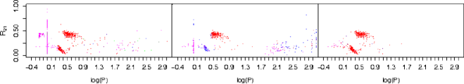
Figure 8: The $R_{21}-\log(P)$ plane of classical Cepheids (red), RVTAU (green), PTCEP (blue) and DMCEP (magenta) in the LMC according to the multistage (left) and GM (middle) classifiers and the OGLE team sample (right, only fundamental and first overtone classical Cepheids in red, and DMCEP in magenta).

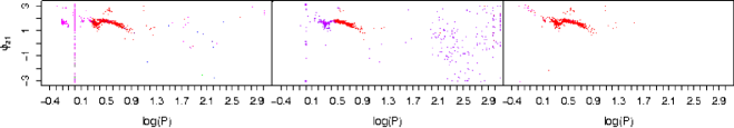
Figure 9: The $\phi_{21}-\log(P)$ plane of classical Cepheids (red), RVTAU (green), PTCEP (blue) and DMCEP (magenta) in the LMC according to the multistage and GM classifiers and the OGLE team sample (only fundamental and first overtone classical Cepheids in red, and DMCEP in magenta).

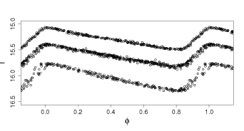
Figure 10: $I$-band light curves of OGLE050131.82-692319.0, OGLE051759.78-691602.5 and OGLE053643.23-701030.7 folded with the periods $P=3.3622$, $P=3.5656$ and $P=3.7675$ respectively and displaced vertically for clarity.

4.3 Eclipsing binaries

Table 8 shows a comparison between the OGLE sample of eclipsing binaries and the samples obtained by our classifiers. We have preferred not to include the subtype classification of eclipsing binaries (EA/EB/EW) because, in our opinion, the boundaries between them are not sufficiently well defined in terms of quantifiable criteria and thus result in large error rates not justified in terms of real classification errors.

The good performance of the classifiers for this problematic class is remarkable. Figures 11 and 12 corresponds to SMC objects classified as eclipsing binaries with a probability above 90% (for the MSBN classifier) because the LMC eclipsing variables were used in the training set and thus, performance estimates based on the same cases used for training would have a strong optimistic bias. The MSBN classifiers recovers 75% of the OGLE sample without incorporating colour information (73% using $B-V$ and $V-I$ and 43% adding 2MASS colours) but, most remarkably, it recovers 97% of the bulge sample by Groenewegen (2005) (95% using $B-V$ and $V-I$ and 92% adding 2MASS colours). These percentages are even larger than those obtained for the LMC on a set of systems used to train the classifier, as explained above.

As was the case with the double mode Cepheids, having used OGLE observations of eclipsing binaries in the definition or training set results in overfitting and a strong tendency to classify other variability types as eclipsing binaries. This can be detected as a sizable number of objects similar to RR Lyrae stars and classical Cepheids mistakenly classified as eclipsing binaries. They are easily detected by the large phase differences between the various harmonics (these objects do not appear in Figure 11 because they have class probabilities well below 90%).

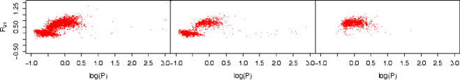
Figure 21: The $R_{21}-\log(P)$ plane of eclipsing binaries for the Galactic Bulge. From left to right, the MSBN and GM samples and the OGLE catalogue.

The lack of systems with sinusoidal light curves and low $R_{21}$ ratio, specially around $\log(P)\approx 0$ is also evident from the plots. This hypothesis is confirmed by two facts: the distribution of the $R_{21}$ ratio amongst OGLE eclipsing binaries misclassified by the MSBN classifier (though multimodal) has the strongest component below $R_{21}=0.2$; second, the astonishing true positive detection rate in the Groenewegen (2005) sample is due to its being composed exclusively of detached systems (see Figure 21), because its main objective was to obtain candidates for distance determination.

As with previous variability types, the classifiers provide candidate lists that include objects not in the published reference samples. In this case, the 90%-confidence lists comprise 3122 candidates in the LMC, 1216 in the SMC and 14610 in the Galactic bulge. Of these, 990 are new candidates in the LMC not in any of the published lists (330 and 11739 in the SMC and Galactic bulge respectively). As a check for these new candidates, we have plotted some of the systems with the longest periods and the largest $R_{21}$ ratios amongst the SMC candidates (see Figure 13). On the left column plots we show confirmed candidates of the category of eclipsing binaries while the rightmost column shows one possible example of instrumental effects (top; the dimming of the star always associated with the end of a series of observations) and one example of a more complicated system with various causes contributing to the light curve variability. As with all previous categories, we do not claim that all these new sources have to be treated as confirmed cases but rather as strong candidates upon which further selection criteria can be applied in order to obtain manageable candidate lists.

Table 8: Number of eclipsing binary systems according to the OGLE and Groenewegen catalogues and correctly identified by the Gaussian Mixtures (GM) and multistage Bayesian networks (MSBN) classifiers presented here. The table lists the number of systems in the two catalogues with a clear counterpart in the OGLE variability database and, subsequently, the fraction of these with available visible and visible+2MASS colours.

Catalogue	Source	Potential detections			GM		MSBN
		NC	+(B)VI	+JHK	NC	+(B)VI	NC	+(B)VI	+JHK
OGLE eclipsing binaries	LMC	2631	2467	210	1613	1528	2296	2072	150
OGLE eclipsing binaries	SMC	1387	1316	153	824	809	1045	967	65
Groenewegen (2005) eclipsing binaries	LMC	173	162	27	80	77	132	108	10
Groenewegen (2005) eclipsing binaries	SMC	16	15	8	8	8	9	8	1
Groenewegen (2005) eclipsing binaries	bulge	3034	2132	1260	2599	1295	2951	2016	1159

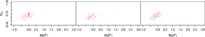
Figure 11: The $R_{21}-\log(P)$ plane of eclipsing binaries for the SMC. From left to right, the MSBN and GM samples and the OGLE catalogue.

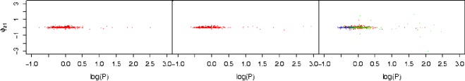
Figure 12: The $\phi_{21}-\log(P)$ plane of eclipsing binaries for the SMC. From left to right, the MSBN and GM samples and the OGLE catalogue.

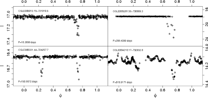
Figure 13: Example light curves of new systems classified as eclipsing binaries and not in the reference samples.

4.4 Long period variables

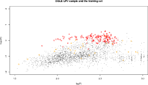
Figure 23: First frequency amplitude vs. $\log(P)$ of Miras (red) and SRs (orange) in the training set and in the OGLE sample (black).

Long period variables (LPVs) constitute the class where the most significant discrepancies are found. As shown in Table 9, the MSBN classifier barely recovers 50% of the LMC OGLE sample of Mira and Semiregular variables. The reason is two-fold: first, many of the OGLE long period variables (17% and 45% in the OGLE LMC and Bulge samples respectively) are missed in the frequency calculation step where the sampling frequency ($\approx 1$ c/d) prevails over the stellar pulsation, thus providing first and subsequent frequencies in error. Second, there is a lack of low amplitude Miras and semiregular stars with periods of less than 150 days in the training set, and those are the main contribution to the missing LPVs. Figure 23 shows a comparison between the first frequency amplitude of Miras and semiregulars in the training set and in the OGLE LMC sample. In this regime, the number of examples is so low that it is indeed less than that of the LBV or Periodically Variable B- and A-type supergiant (PVSG) classes, the main contributors to the False Negative Rate (misclassified Mira and Semiregular stars according to the OGLE sample). Therefore, there is a clear need to extend the training set representation of the Mira and Semiregular classes in this region of the parameter space. The situation is different for the Matsunaga et al. (2005) and Groenewegen & Blommaert (2005) candidate lists where the true positive rates increase to 87%. We interpret this increase in performance as a confirmation of the hypothesis put forward above given the absence of low amplitude variables with periods below $\log P\approx 2.2$ in these lists. Unfortunately, the lack of low period-low amplitude Miras and semiregulars is not visible in Figure 14 due to the crowd of stars in the plot.

As expected, the inclusion of Johnson photometry in the inference process corrects the low performance of the classifiers in the OGLE LMC case and increases the TPR up to 94% (98% when 2MASS photometry is included). This effect can be easily understood given the strong relevance (in the sense commonly accepted by the Statistical Learning community) of these attributes. Surprisingly though, it also results in a small performance degradation (2–5%) in the bulge samples by Matsunaga et al. (2005) and Groenewegen & Blommaert (2005).

Using a confidence threshold of 90%, we find 67 new candidates in the LMC and 990 in the Galactic Bulge. As in all previous cases, visual inspection of the position of the new candidates in several 2D projections confirms the adequacy of their parameters for the class definitions in the training set and reference samples. Random inspection of some candidates indicates that most of the new candidates are semiregular pulsators often affected by long term trends in the mean brightness and several frequency components.

Table 9: Number of long period variables (LPV) according to the Matsunaga et al. (2005) and Groenewegen & Blommaert (2005) catalogues, and correctly identified by the Gaussian Mixtures (GM) and multistage Bayesian networks (MSBN) classifiers presented here. The table lists the number of systems in the two catalogues with a clear counterpart in the OGLE variability database and, subsequently, the fraction of these with available visible and visible+2MASS colours.

Catalogue	Source	Potential detections			GM		MSBN
		NC	+(B)VI	+JHK	NC	+(B)VI	NC	+(B)VI	+JHK
OGLE LPV	LMC	3472	2735	2552	407	2060	1718	2576	2508
OGLE LPV	bulge	273	129	90	84	85	69	65	67
Miras (Matsunaga et al. 2005)	bulge	1882	1284	733	1498	1186	1642	1052	627
Miras (Groenewegen $\&$ Blommaert, 2005)	bulge	1999	1276	737	1648	1178	1734	1038	632

Figure 14: The $A_{11}-\log(P)$ plane for long period variables in the LMC according to (from left to right) the multistage and GM classifiers and the OGLE team sample.

4.5 Multiperiodic variables

It is clear that both classifiers perform well for the majority of the classes considered above. However, most of these classes contain monoperiodic (radial) pulsators, or eclipsing binaries. Our classification scheme also included several multiperiodic classes. Multiperiodic variables are amongst the most scientifically interesting classes in relation to asteroseismic studies of the stellar structure and evolution, see e.g. Kurtz (2006) for a review. Nevertheless, they have not been thoroughly studied in the OGLE variable databases.

4.5.1 Pulsating B-stars in the Magellanic clouds

We could not compare our results for those classes with existing results in such an extensive way. These classes have been much less studied up to now, mainly because their detection is less obvious in the OGLE data. Since they are relevant for asteroseismology, we present here the results obtained with both classifiers for $3$ classes of massive intrinsically bright multiperiodic pulsators: $\beta$-Cephei stars (BCEP), slowly pulsating B-stars (SPB), and periodically variable super giants (PVSG). We limit ourselves to these classes, since the other well-known multiperiodic classes contain much fainter stars, making their detection even more difficult in the OGLE data for the Magellanic clouds. Because single-band light curve information is usually not sufficient to identify those objects in an unambiguous way, we only consider here the classification results obtained with the additional colour attributes B-V (and V-I) included for both classifiers. We also place the new candidate variables in the HR diagram. This could be done only for the LMC and SMC variables, since B-V colours, V magnitudes and distances are only available for those objects. For the Bulge data, only V-I and $2MASS$ colours are available, and the distance is unknown. Moreover, the V-I colours for the Bulge have proven to be less reliable, as mentioned earlier. However, the Bulge sample is larger and contains brighter objects, so detection of those variables (based on their light curve) is more likely in this sample (if they are present). We present some of the best candidates in the Bulge in the next section, by showing their phase plots (made with the dominant frequency we detected) and listing some of their light curve parameters. The samples are much too large to check all the candidates (this is out of the scope of this work), but the full classification results with both classifiers will be made available electronically.

The best candidate pulsators are shown in the HR-diagrams for both the Small and the Large Magellanic cloud. The distances used to construct the diagrams are as follows: $D(SMC)=60.6\pm 2.97$ kpc (Hilditch et al. 2005), and $D(LMC)=48.1\pm 3.70$ kpc (Macri et al. 2006). To convert the $V$ magnitudes of the objects into absolute luminosities $\log(L/L_{\sun})$, we used the value of $4.75$ for the Sun’s absolute bolometric magnitude. Bolometric corrections and effective temperatures ($\log T_{eff}$) were obtained using the corrected empirical transformations described in Flower (1996). Typical errors for $\log(L/L_{\sun})$ and $\log T_{eff}$ have been derived, taking the uncertainties on the distance, the V magnitudes and the B-V colours into account. Theoretical instability strips for $\beta$-Cephei (Stankov & Handler 2005), SPB (de Cat 2002) and PVSG stars (Lefever et al. 2007) are shown. For details on the derivation of the strips, we refer to Miglio et al. (2007), Saio et al. (2006), and references therein. The PVSG instability strip is for post-TAMS models with non-radial mode degree values $l=1$ and $l=2$. The SPB and BCEP instability strips are obtained with the OP opacity tables (giving the widest strips), with metallicity values Z ranging from $0.005$ to $0.02$, and non-radial mode degree values $l=0$ to $3$. Overshooting is included ($\alpha=0.2$ Hp), and stellar masses up to $18M_{\sun}$ were considered. Only main sequence models were included, and an initial hydrogen mass fraction $X=0.7$ has been used. We plot instability strips for different Z values, to show how the instability domains are expected to shrink when Z decreases, and to show the difference in metallicity between the LMC and the SMC. For the plots of the results for the LMC, the SPB and BCEP instability strips are shown for $Z=0.02$ (outer borders) and $Z=0.01$ (inner borders). For the plots of the results for the SMC, the SPB and BCEP instability strips are shown again for $Z=0.02$ (outer borders), and also the SPB instability strip for $Z=0.005$ (inner borders). The BCEP instability strip for $Z=0.005$ disappears (Miglio et al. 2007). The PVSG instability strip in both cases corresponds to $Z=0.02$. The position in the HR diagram of the new candidates found with our classifiers, relative to these instability strips, provides a reliability check of the excitation models.

The whole sample of variable stars in the LMC and SMC with colours available is shown in Figures 15 and 16 (small black dots).

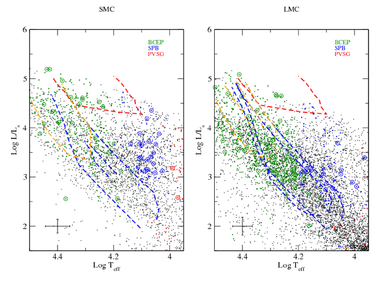
Figure 15: HR-diagram for both the SMC and LMC. The black dots represent the total sample of variable stars for which colours were available. The coloured dots represent those variables classified as BCEP, SPB, and PVSG with the MSBN method. A lower limit of $0.5$ was used for the class probabilities. The encircled dots (in the respective class colours) represent objects classified as such with both classifiers. The BCEP instability strips are plotted in orange for visibility. For the right panel, the SPB and BCEP instability strips are shown for $Z=0.02$ (outer borders) and $Z=0.01$ (inner borders). For the left panel, the SPB and BCEP instability strips are shown again for $Z=0.02$ (outer borders), and also the SPB instability strip for $Z=0.005$ (inner borders). The PVSG instability strip corresponds to $Z=0.02$.

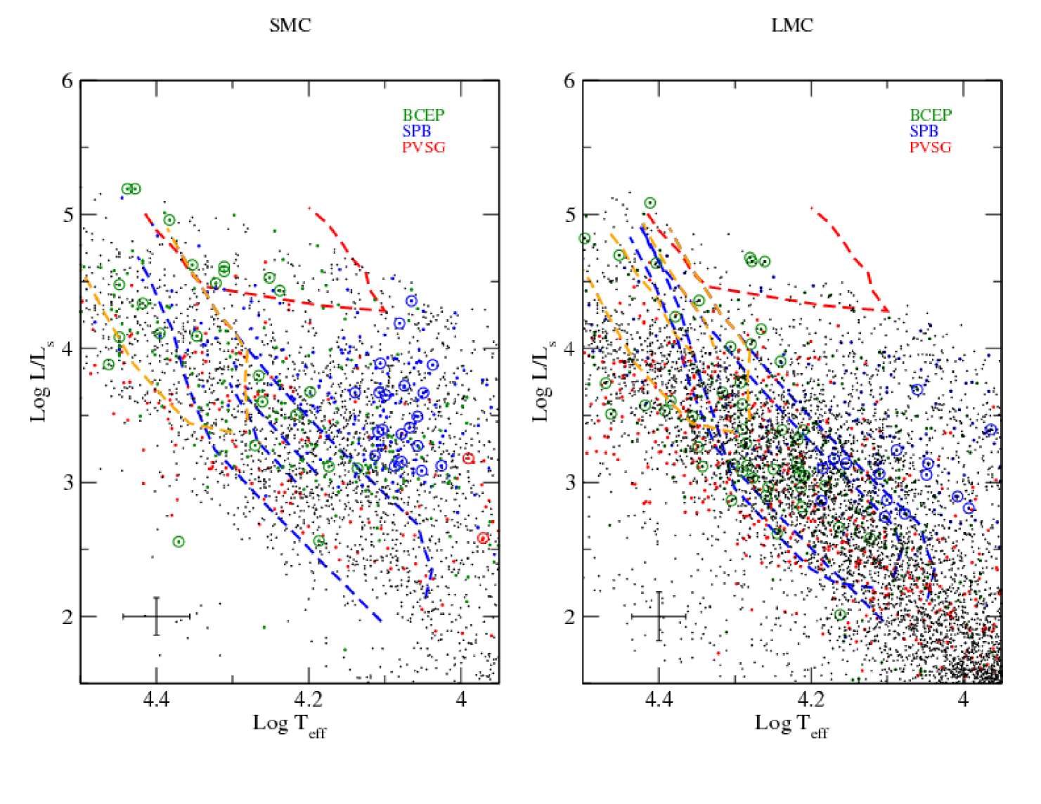
Figure 16: HR-diagram for both the SMC and LMC. The black dots represent the total sample of variable stars for which colours were available. The coloured dots represent those variables classified as BCEP, SPB, and PVSG with the GM method. An upper limit of $3.5$ was used for the Mahalanobis distance to the class centers. The encircled dots (in the respective class colours) represent objects classified as such with both classifiers. The BCEP instability strips are plotted in orange for visibility. For the right panel, the SPB and BCEP instability strips are shown for $Z=0.02$ (outer borders) and $Z=0.01$ (inner borders). For the left panel, the SPB and BCEP instability strips are shown again for $Z=0.02$ (outer borders), and also the SPB instability strip for $Z=0.005$ (inner borders). The PVSG instability strip corresponds to $Z=0.02$.

The new candidate pulsators for the $3$ B-type classes, and the corresponding instability strips, are shown in colour. Note that the BCEP instability strip is shown in orange (BCEP candidates are in green), for visibility. Objects having the same class label with both classifiers are encircled.
Since every object will be assigned to one of the classes in our supervised classification scheme, contamination in the classification results is to be expected, e.g., not all stars classified as belonging to one of the BCEP, SPB, or PVSG classes will be real members of those classes. This is not a drawback, however, since our class assignments are probabilistic, and allow us to impose limits on the class probabilities. This way, we can select the most probable candidates only.
The MSBN classifier provides relative probabilities for an object to belong to any of the classes. Figure 15 shows all the objects having a probability of belonging to the BCEP, SPB, or PVSG classes higher than $0.5$, obtained with this classifier. Note that most SPB candidates are situated above their instability domains (higher luminosity), taking into account the errors bars. Their position on the temperature scale is within the expected range, because the B-V colour was used as a classification attribute. Objects far from this pre-defined range are given a low class-probability and will not be present in our selections.
The GM classifier provides relative probabilities, and, in addition, the Mahalanobis distance to the center of the most probable class. This distance can effectively be used to retain only the objects that are not too far from the class center in a statistical sense. It can be used together with the probabilities, in order to select the best candidates. For the GM classifier, using only the probability values is usually insufficient to select the best candidates. Consider the case e.g., where the probability for one class is $99\%$. This high probability value seems to indicate a very certain class assignment. However, these are only relative probabilities, and, even though the probability for the class is very high, the object might still be very far away from the class center. If this is the case, the Mahalanobis distance will have a large value, and one has to conclude that the object is not a good candidate to belong to the class after all. To guide us in choosing a meaningful cutoff value for the Mahalanobis distance $D$, we can use the fact that $D^{2}$ is chi-square distributed for multinormally distributed classification parameters (the basis of the GM classifier). The number of degrees of freedom $p$ is equal to the number of classification attributes. Given the Mahalanobis distance $D$ to the class, we can use this property to test the likelihood of finding a distance larger than $D$, under the assumption that the object belongs to the class. Note that for $p>2$, which is the case for the GM classifier, the chi-square distribution will not be monotonically decreasing with increasing value of $D^{2}$. This means that very small values of $D$ are unlikely as well, and we should perform a two-tailed hypothesis test.
Figure 16 shows the HR diagrams with the results of the GM classifier, for the SMC and LMC, again with the variables classified as BCEP, SPB, PVSG, and their respective instability strips shown in colours. All these candidate variables have a Mahalanobis distance to the class center of less than $3.5$ (dimensionless, similar to a distance in terms of sigma in the one dimensional case). Objects having the same class label with both classifiers are encircled. The same remarks as for the MSBN results apply here: most SPB candidates are situated at higher luminosities than expected for this type of variable.

The g-mode and p-mode pulsations in SPB and BCEP stars, respectively, are caused by the $\kappa$-mechanism, acting in the partial ionization zones of iron-group elements. This mechanism thus strongly depends on the presence of those heavy elements, and hence on the metallicity of the stellar environment. It was previously believed that the BCEP and SPB instability strips nearly disappear for metallicities Z smaller than $0.006$ and $0.01$ (Pamyatnykh 1999). However, the recent results presented in Miglio et al. (2007), and used in this work, show that an SPB instability strip can still exist for Z as low as $0.005$. They do not predict BCEP pulsations at such a low metallicity value, though. Since the metallicity of the SMC is estimated to be between $Z=0.001$ and $Z=0.004$ (Maeder et al. 1999), we would not expect to find any BCEP or SPB pulsations here. However, several independent investigations have shown that SPB and BCEP pulsators are nevertheless present in low metallicity environments such as the LMC and even the SMC. Examples are given in Kołaczkowski et al. (2004), Pigulski & Kołaczkowski (2002), Karoff et al. (2008) and Diago et al. (2008). Our classification results for the OGLE LMC and SMC data support those conclusions and suggest that even more candidates than found so far exist. In total, we find 15 SPB and 48 BCEP candidates in the LMC, and 20 SPB and 24 BCEP candidates in the SMC. As is expected, more pulsators are found in the metal-richer LMC. Note that a large number of BCEP candidates are situated in the higher parts of the SPB instability strips, both for the SMC and LMC. Overlap between the instability strips is present in that area, and stars can show similar pulsation characteristics there. The relatively large errors on the position in the HR diagram (see the crosses in the plots) should be kept in mind also. As mentioned above, we see that SPB candidates appear at higher luminosities than expected, taking into account the error bars. This is the case for both the LMC and SMC, and with both the MSBN and GM classification results. Since the Magellanic clouds contain evolved stars, we suggest that some of these SPB candidates could in fact be B-type PVSG stars. In Waelkens et al. (1998), it was suggested that the pulsations in those stars could be gravity modes excited by the $\kappa$-mechanism, similar to the BCEP and SPB stars. This is confirmed in Lefever et al. (2007), where a sample of B-type PVSG stars is investigated in detail. Typical pulsation periods for those variables are in the range $1-20$ days, so an overlap with the typical period range for SPB stars is present. One may wonder why those objects are then not classified as PVSG with our classifiers. The PVSG class is a very heterogeneous class, containing both B-type and A-type pulsators (note that the shown PVSG instability strip is only for B-type stars). Moreover, they show pulsations over a wide range of frequencies and amplitudes. This translates into a large spread of this class in our classification parameter space. The PVSG class overlaps with the SPB class in parameter space, but has a lower probability density of objects at the locations overlapping with the SPB class. This implies that a potentially good PVSG candidate, but with properties close to those of SPB stars, will most likely be classified as SPB and not as PVSG. Candidate PVSG variables are shown in Figure 15 and Figure 16. There is a large discrepancy between the numbers found by the MSBN and the GM classifiers. This is a consequence of the poor definition of this class. A visual check of the phase plots did not reveal convincing candidates, in addition to the high-luminosity BCEP and SPB candidates.

The SPB and BCEP candidates present in our selection lists and having the same classification with both classifiers are most likely good candidates. For those objects, we made phase plots with the dominant frequencies ($f_{1}$) and list some of their light curve properties. Note that the typical pulsation frequencies for SPB stars are situated around $1$ c/d. The $1$ c/d frequency is unfortunately also a spurious frequency often detected in the OGLE data, due to the daily gaps in the observations (the OGLE window function). Since this frequency is often significant, care must be taken not to interprete these as real pulsation frequencies. We could exclude the most likely spurious detections by checking the phase plots: if the plots show clear gaps, we are probably dealing with a spurious frequency (though in some cases, we might have a real pulsation frequency very close to $1$ c/d).

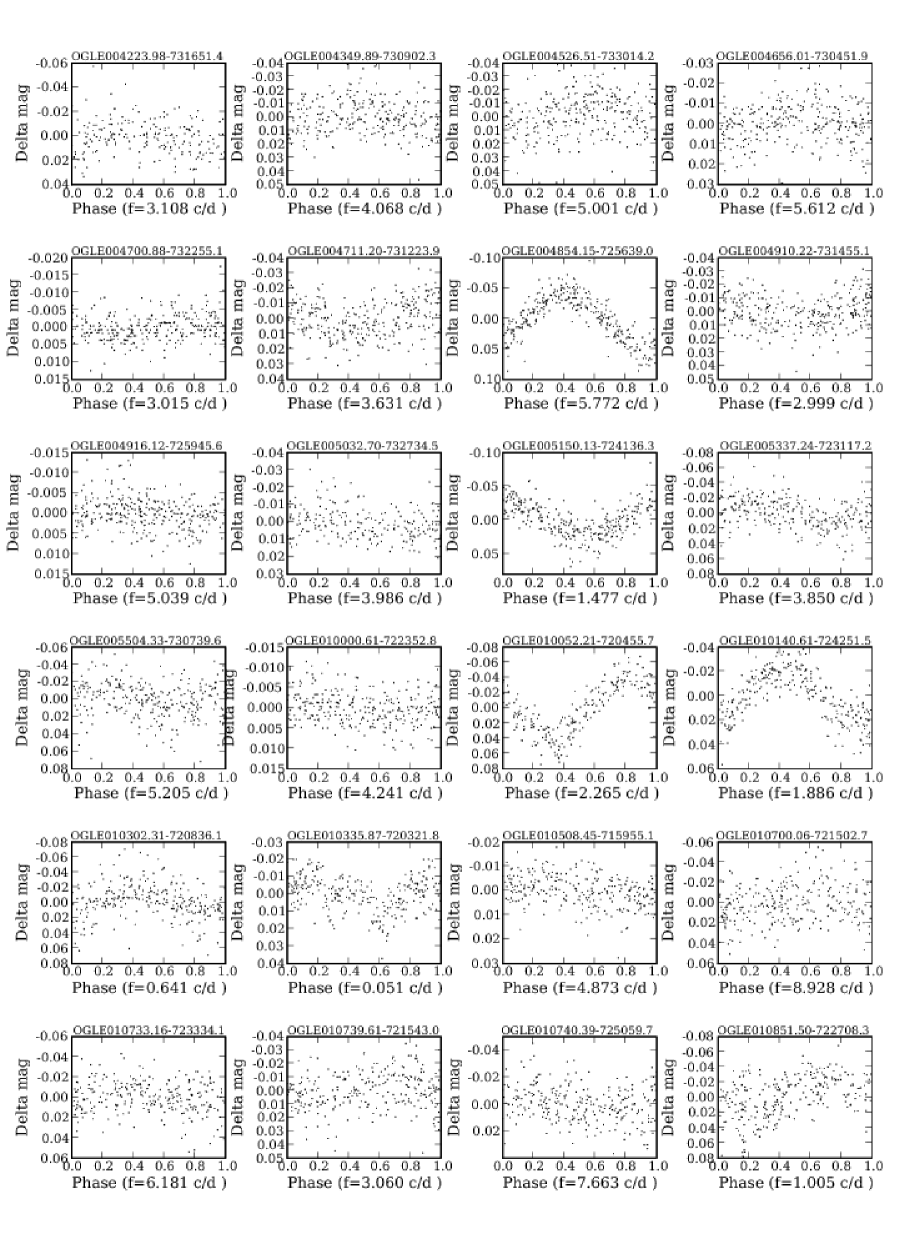
Figure 25: Phase plots of variables in the SMC classified as BCEP with both the MSBN and the GM method. The OGLE identifier is shown, and the dominant frequency, used to fold the light curves, in units of cycles per day (c/d).

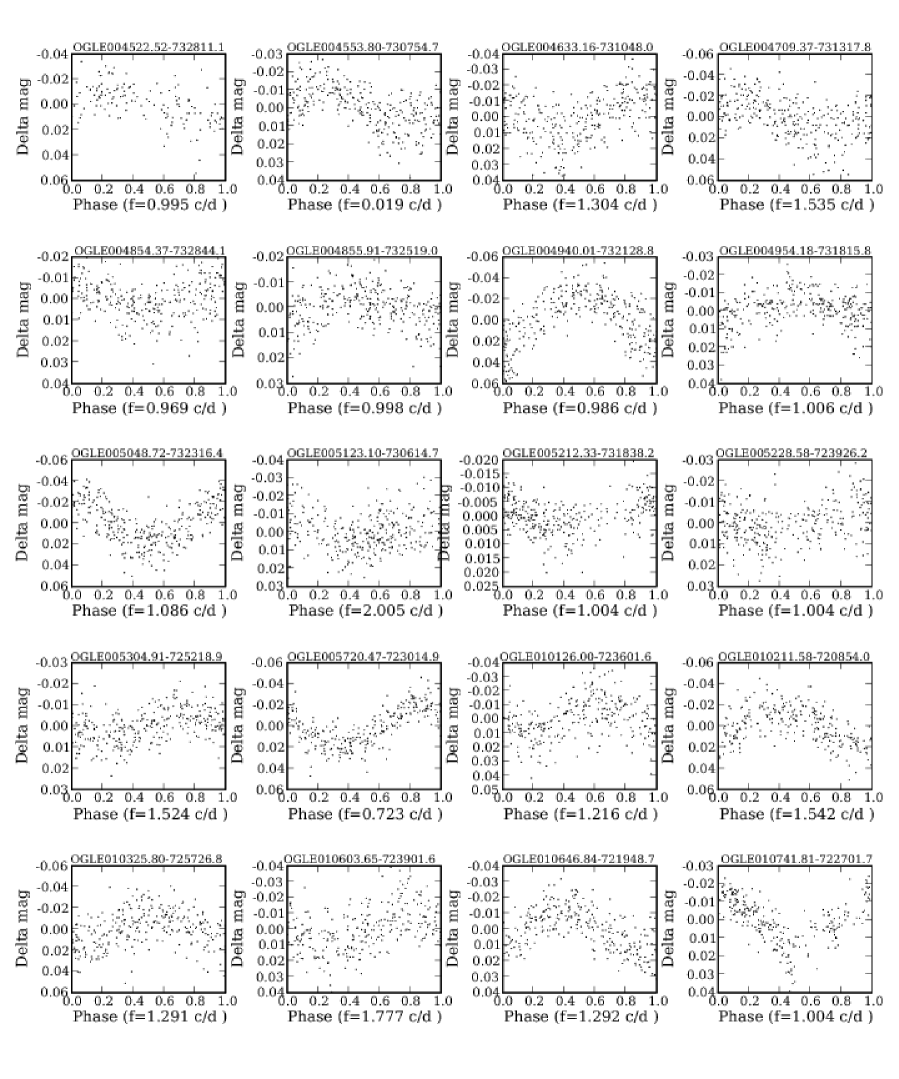
Figure 26: Phase plots of variables in the SMC classified as SPB with both the MSBN and the GM method. The OGLE identifier is shown, and the dominant frequency, used to fold the light curves, in units of cycles per day (c/d).

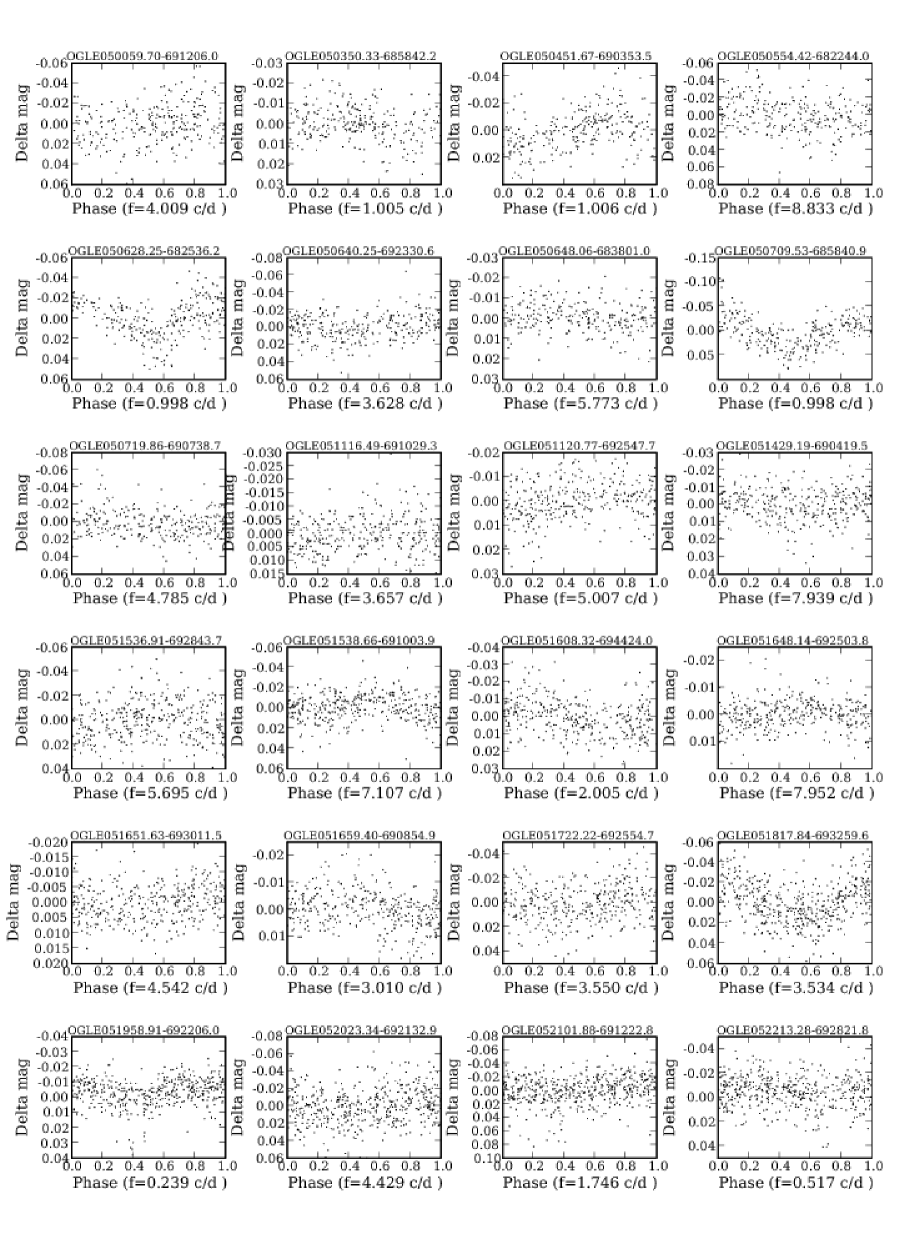
Figure 27: Phase plots of variables in the LMC classified as BCEP with both the MSBN and the GM method. The OGLE identifier is shown, and the dominant frequency, used to fold the light curves, in units of cycles per day (c/d).

Figure 25 and Figure 26 show phase plots of candidate BCEP and SPB stars in the SMC. The OGLE identifier and the value of the dominant frequency are shown. Some of their properties are listed in Table 11 and Table 12 respectively. Figures 27 to 29 show the phase plots of candidate BCEP and SPB stars in the LMC data. Their properties are listed in Table 13 and Table 14. The tables also list the value of the second detected frequency $f_{2}$, one of the classification attributes used.

4.5.2 The Galactic bulge

To the best of our knowledge, the OGLE team only produced a candidate list for the class of $\delta$ Scuti pulsators, in the first field of the bulge and, unfortunately, only of the high amplitude candidates, usually monoperiodic (see for example McNamara, 2000). Ten out of 11 systems listed in the catalogue by Mizerski and available to us are correctly identified as $\delta$ Scuti stars by the MSBN classifier and the eleventh (bul_sc1_1323) has a period of 6.7 hours, which is slightly above the range of periods found for this class. The system is classified as RRD. With the GM classifier, 7 out of 11 systems are classified as $\delta$ Scuti stars.

Pigulski (private communication) has kindly provided us with candidate lists of several types of multiperiodic pulsators prior to publication, as well as an extended list of high amplitude $\delta$ Scuti (HADS) stars across all OGLE bulge fields (Pigulski et al. 2006). We have applied the same procedure described above to these lists in order to assess the performance of the classifiers in detecting multiperiodic pulsators. In the following, we describe the results obtained with the time series attributes alone since the inclusion of $V-I$ in the bulge has proved detrimental to the classifiers, probably due to insufficient dereddening.

Table 10 shows the main contributors to the confusion matrix constructed by assuming Pigulski’s class assignments. His results are grouped in three catalogues: the high amplitude $\delta$ Scuti stars (HADS) group, the mixed slowly pulsating B/ $\gamma$ Doradus group, and the $\beta$ Cephei/$\delta$ Scuti group. Again, the classifiers are capable of retrieving a significant fraction of the HADS candidates (63-78% with the GM and MSBN classifier respectively). These numbers decrease for the mixed groups (11-61% for the BCEP/DSCUT list and 70-37% for the SPB/GDOR one with the GM and MSBN classifier respectively). Note the low correspondence with the BCEP/DSCUT list for the GM results and with the GDOR/SPB list for the MSBN results. This confusion is inherently connected to the physical properties for the stars in these classes, which imply overlap in the characteristics of their pulsations. An example is the occurence of both short-period p-modes and long-period g-modes in BCEP stars (e.g. Handler et al. 2004, 2006) and the only vague separation of the p-mode frequencies of evolved BCEP and DSCUT stars, from the g-mode frequencies of young SPB and GDOR stars, respectively, particularly when frequency shifts due to rotation are taken into account.

Table 10: Summary of the class assignments for objects in Pigulski’s lists (private communication) for both the GM and the MSBN classifier.

		GM					MSBN
Pigulski class	Potential detections	PVSG	BCEP	DSCUT	GDOR	SPB	PVSG	BCEP	DSCUT	GDOR	SPB
HADS	190	10	6	119	2	0	10	2	147	0	1
BCEP-DSCUT	225	3	12	12	73	16	12	28	109	16	11
SPB-GDOR	623	22	27	4	194	239	149	7	41	37	191

4.5.3 New candidates in the Bulge

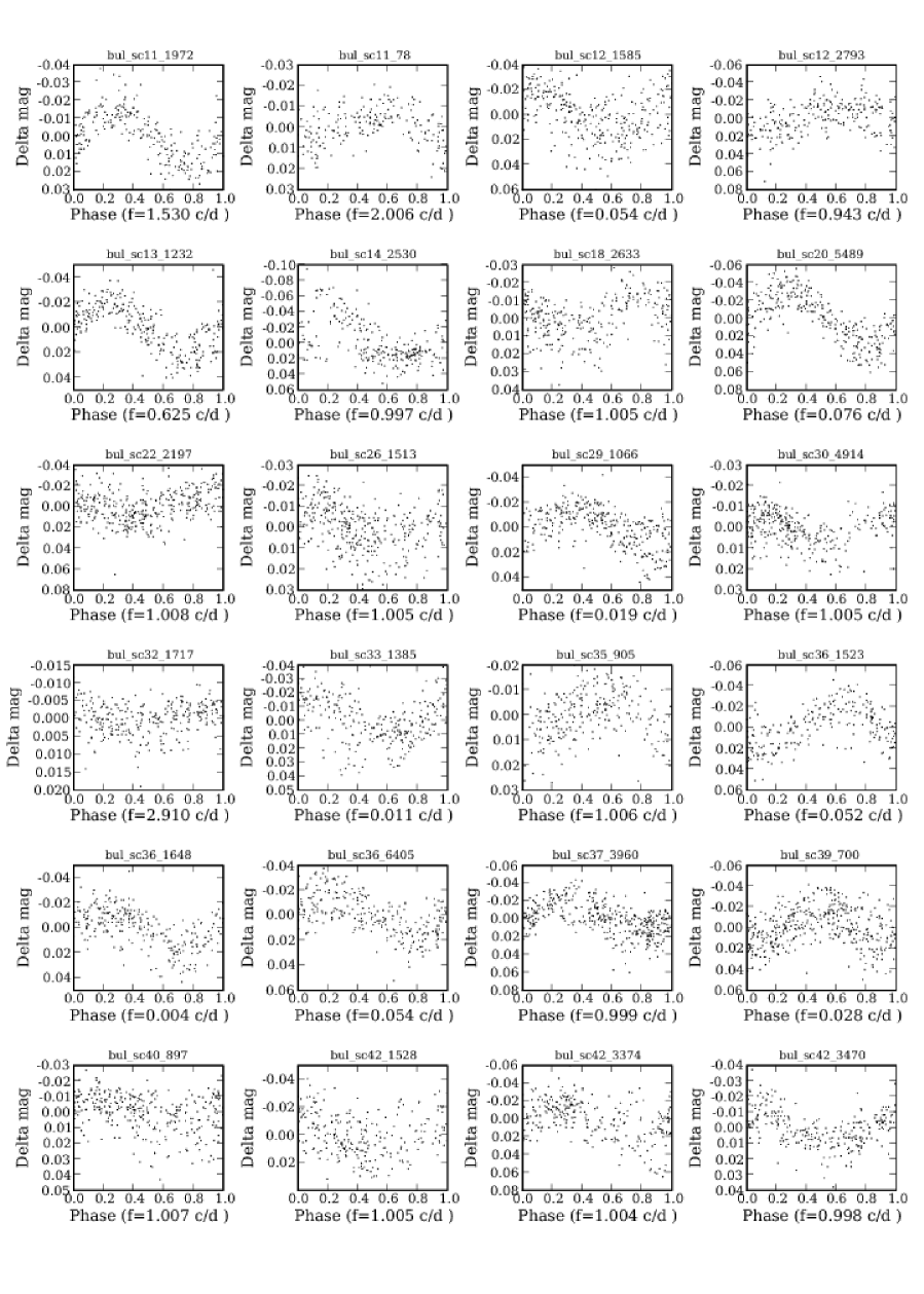
Figure 30: Phase plots of variables in the Galactic Bulge classified as SPB with both the MSBN and the GM method, and not present in the list of Pigulski. The OGLE identifier is shown, and the dominant frequency, used to fold the light curves, in units of cycles per day (c/d).

Here, we present a selection of Bulge objects classified as DSCUT, BCEP, SPB or GDOR, with both classifiers, and not present in the respective combination lists made by Pigulski. Figures 30 to 39 show their phase plots made with $f_{1}$. The OGLE Bulge identifiers are shown, and the values of $f_{1}$ in cycles per day. Light curve parameters and V-I colour indices are listed in Tables 15 to 19. The most obvious spurious detections (having a value of $f_{1}$ very close to $1$ c/d) were removed from our selections. We stress that these are candidate lists obtained with probabilistic class assignments. Further investigation is needed to reach more certainty about the true nature of those objects. Significant overlap is present between the pulsation properties of the GDOR/SPB and BCEP/DSCUT classes, which is the reason why Pigulski did not make the distinction in his lists. We expect this to be reflected in our candidate lists as well, e.g. some SPB candidates might be GDORs and vice versa, and the same for the BCEP/DSCUT classes. Apart from some inherent overlap between these classes, this is mainly a limitation of the current classification attributes that we can use (e.g. the absence of a good colour), and the quality of the light curves.
As opposed to selections made with extractor methods, we can have objects in our list having rather atypical light curve parameters for that particular class. These can be borderline cases, and in some cases, misidentifications. As was mentioned earlier, however, stronger limits can be imposed on the class probabilities and/or the Mahalanobis distance, to retain only the most typical candidates. In doing so, the samples will be purer, but, on the other hand, interesting border cases can be missed.

5 Conclusions.

In the past few years, the world of astronomy has seen a revolution taking place with the advent of massive sky surveys and large scale detectors. This revolution cannot be fully exploited unless automatic methods are devised in order to preprocess the otherwise unmanageably large databases. Otherwise, the efforts of the astronomical community will have to focus on repetitive uninteresting data processing rather than in the solution of the scientific questions that motivate the efforts. In this work we have presented a scenario with many interesting open questions for research (distance estimator calibration, stellar interiors, galactic evolution…), i.e. that of stellar variability, where automatic procedures for data processing can help astronomers concentrate on the solution to these problems. We have developed automatic classifiers that, in a matter of seconds or minutes, can automatically assign class probabilities to hundreds of thousands of variable objects, and we have proved that these probabilities are highly reliable for the set of classical variables best studied in the literature. These experiments are repeatable and thus free from human subjectivity. The classifiers show minor discrepancies with the classifications used as a reference in this work (as explained in previous sections) and these discrepancies, when due to the classifiers themselves, need to be corrected for. Until then, users of the publicly available classifiers have to be aware of these minor pitfalls when interpreting their results.

The results presented here suggest that further steps can be taken in the analysis of the resulting samples. Two obvious steps are the search for correlations between subsets of attributes not necessarily of dimension 2, and the study of density plots and clustering results in order to explore the substructure within each variability class. This is the subject of ongoing research in the framework of the CoRoT, Kepler and Gaia missions.

The training set and the classifiers are only the first operational versions developed for the optimization of on-going and future databases such as CoRoT, Kepler or Gaia. Obviously, both the training set and the classifiers will greatly benefit from the analysis of these future databases, especially for those classes underrepresented in terms of the real prevalences. This is where the improvement and correction of the discrepancies mentioned in the previous paragraph will take place. They must be oriented towards obtaining a class definition (training) set that better reproduces the real probability densities in parameter space (the probability of a variable object of class $C_{k}$ having a certain set of attributes such as frequencies, amplitudes, phase differences, colours, etc). Furthermore, it must be made more robust against overfitting by combining data from various surveys/instruments in such a way that the sampling properties (including measurement errors) have as little an impact on the inference process as possible. We believe that this paper is a crucial starting point in the sense that we have proved the validity of the classifier predictions, and, at the same time, we have identified and pointed out the source of its limitations, thus showing the path to more complete and accurate classifiers. Obviously, it is in the non-periodic and rarer classes that there is more room for improvement.

Finally, there is ongoing development of new versions of the classifiers adapted to handle spectral information making use of VSOP data (Dall et al. 2007) and including one of the features of Bayesian Networks that make them especially suitable for their integration in the framework of Virtual Observatories, i.e. their capacity to draw inferences based on incomplete (missing) data. We strongly believe that the probabilistic foundations of these models (at the basis of these capabilities) provide astronomers with explanations of the inference process very much in line with the reasoning usually used in astronomy.

In this work We have concentrated on the validation of the developed classifiers, using the OGLE database. This database contains a large number of light curves of different variability types. Existing extractor-type results for the classical pulsators and eclipsing binaries allowed us to judge the quality of our classification results. Our classifiers also identified candidate new members for some of those classes. Little had been done up to now on the multiperiodic pulsators, the most interesting targets from an asteroseismological point of view. The OGLE data are not optimally suited to study those variables, but some types could be studied and discovered. Our classifiers have identified $107$ candidate B-type pulsators (SPB, BCEP and PVSG) in the Magellanic clouds. Those candidates were placed on the HR diagram, to see how they are situated with respect to the instability strips of B-type pulsators. This allowed us to conclude that the present instability computations are incomplete and that their improvement probably needs new input physics. In practice, we provide here a list of new candidate variables of multiperiodic classes (DSCUT, BCEP, SPB and GDOR), including several in the Bulge. A more in-depth analysis of these candidates is needed, but this is outside the scope of this classification work.

Figure 17: The $R_{21}-\log(P)$ plane of RRAB (red), RRC (green) and RRD stars (blue) in the Galactic Bulge, according to the multistage Bayesian networks (left) and Gaussian Mixtures classifiers (middle) and the OGLE catalogue (right).

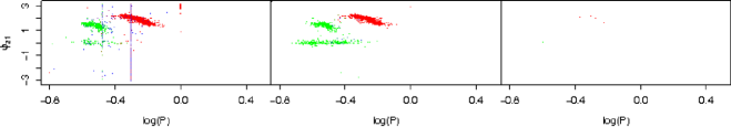
Figure 18: The $\phi_{21}-\log(P)$ plane of RRAB (red), RRC (green) and RRD stars (blue) in the Galactic Bulge, according to the multistage Bayesian networks (left) and Gaussian Mixtures classifiers (middle) and the OGLE catalogue (right).

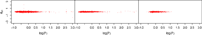
Figure 22: The $\phi_{21}-\log(P)$ plane of eclipsing binaries for the Galactic Bulge. From left to right, the MSBN and GM samples and the OGLE catalogue.

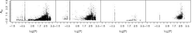
Figure 24: The $A_{11}-\log(P)$ plane of long period variables for the Galactic Bulge. From left to right, the MSBN and GM samples and the Mizerski and Groenewegen catalogues.

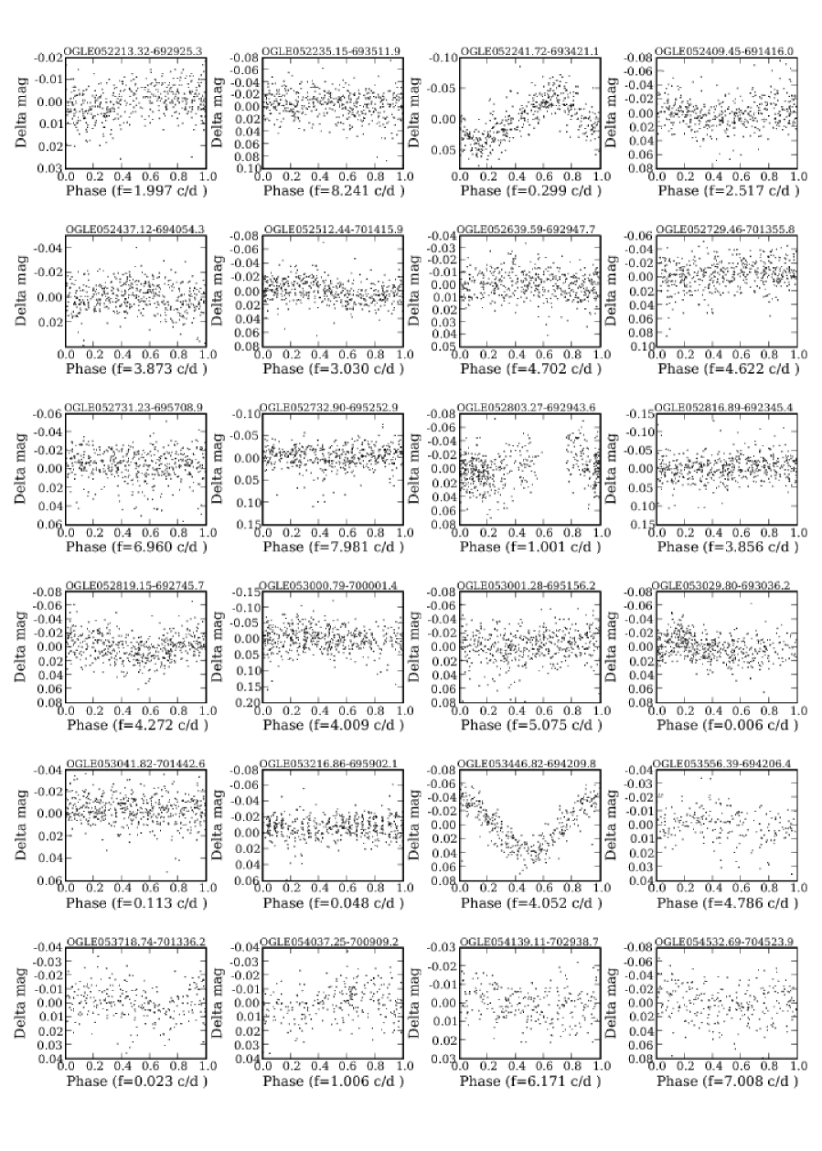
Figure 28: Phase plots of variables in the LMC classified as BCEP with both the MSBN and the GM method. The OGLE identifier is shown, and the dominant frequency, used to fold the light curves, in units of cycles per day (c/d).

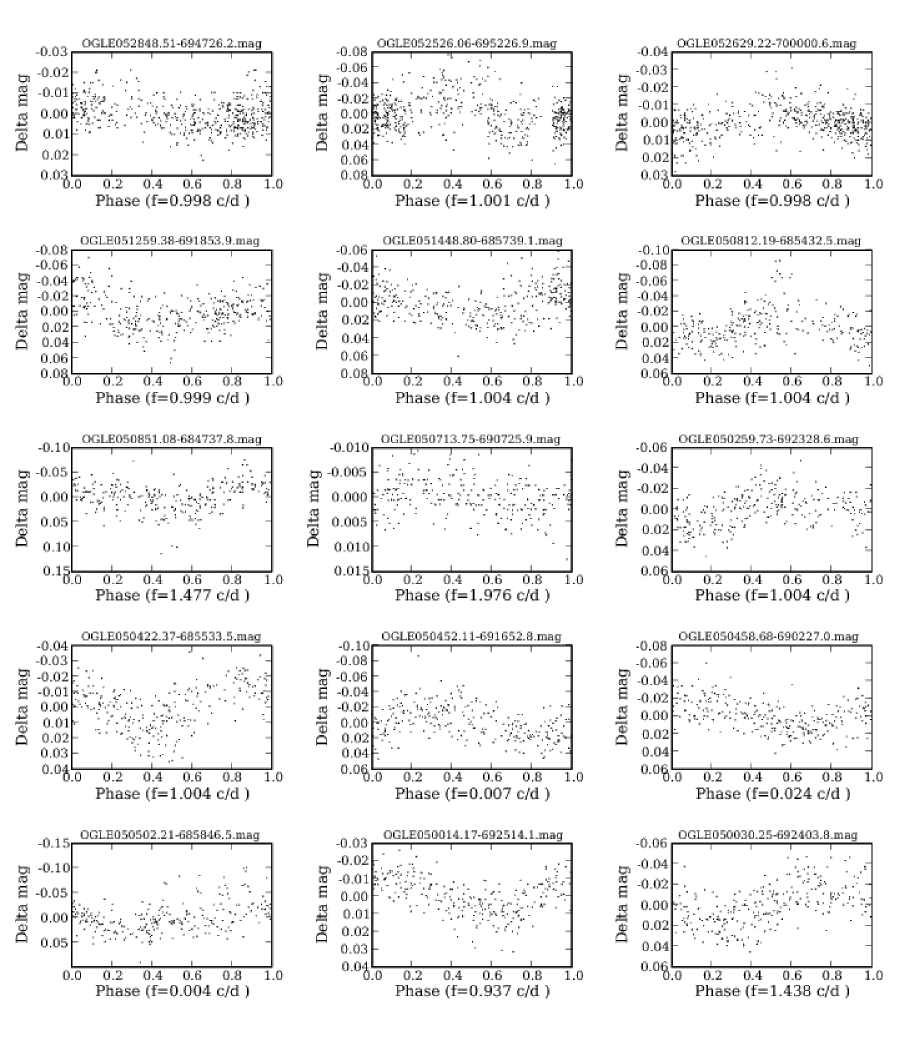
Figure 29: Phase plots of variables in the LMC classified as SPB with both the MSBN and the GM method. The OGLE identifier is shown, and the dominant frequency, used to fold the light curves, in units of cycles per day (c/d).

Table 11: Basic light curve and physical properties of SMC stars classified as BCEP with both the MSBN and the GM method. The dominant frequency $f_{1}$, the second frequency $f_{2}$, the effective temperature $\log T_{eff}$ and the luminosity $\log(L/L_{\sun})$ are listed. The estimated precision on the frequencies is about $0.001$ c/d or smaller. Note that $\log T_{eff}$ and $\log(L/L_{\sun})$ are listed with more digits than the estimated precision, with the only purpose to allow readers to locate the objects in the HR diagrams. The same remark applies to the following tables also. Several of these stars might be evolved pulsators, termed PVSG here, rather than BCEP.

Object identifier	$f_{1}$ ($c/d$)	$f_{2}$ ($c/d$)	$\log T_{eff}$	$\log(L/L_{\sun})$
OGLE004223.98-731651.4	$3.108$	$3.124$	$4.31$	$4.58$
OGLE004349.89-730902.3	$4.068$	$7.151$	$4.38$	$4.96$
OGLE004526.51-733014.2	$5.001$	$7.521$	$4.19$	$2.56$
OGLE004656.01-730451.9	$5.612$	$8.576$	$4.42$	$4.34$
OGLE004700.88-732255.1	$3.015$	$9.123$	$4.25$	$4.53$
OGLE004711.20-731223.9	$3.631$	$3.735$	$4.22$	$3.51$
OGLE004854.15-725639.0	$5.772$	$1.006$	$4.27$	$3.28$
OGLE004910.22-731455.1	$2.999$	$0.135$	$4.31$	$4.61$
OGLE004916.12-725945.6	$5.039$	$4.986$	$4.37$	$2.56$
OGLE005032.70-732734.5	$3.986$	$5.609$	$4.35$	$4.09$
OGLE005150.13-724136.3	$1.477$	$0.739$	$4.46$	$3.88$
OGLE005337.24-723117.2	$3.850$	$0.001$	$4.26$	$3.60$
OGLE005504.33-730739.6	$5.205$	$5.410$	$4.14$	$3.10$
OGLE010000.61-722352.8	$4.241$	$3.008$	$4.35$	$4.62$
OGLE010052.21-720455.7	$2.265$	$2.006$	$4.40$	$4.11$
OGLE010140.61-724251.5	$1.886$	$0.943$	$4.45$	$4.08$
OGLE010302.31-720836.1	$0.641$	$0.298$	$4.32$	$4.49$
OGLE010335.87-720321.8	$0.051$	$0.355$	$4.43$	$5.19$
OGLE010508.45-715955.1	$4.873$	$2.251$	$4.20$	$3.67$
OGLE010700.06-721502.7	$8.928$	$7.743$	$4.27$	$3.80$
OGLE010733.16-723334.1	$6.181$	$1.409$	$4.17$	$3.12$
OGLE010739.61-721543.0	$3.060$	$1.002$	$4.24$	$4.43$
OGLE010740.39-725059.7	$7.663$	$1.057$	$4.44$	$5.19$
OGLE010851.50-722708.3	$1.005$	$0.010$	$4.45$	$4.48$

Table 12: Basic light curve and physical properties of SMC stars classified as SPB with both the MSBN and the GM method. The dominant frequency $f_{1}$, the second frequency $f_{2}$, the effective temperature $\log T_{eff}$ and the luminosity $\log(L/L_{\sun})$ are listed. Several of these stars might be evolved pulsators, termed PVSG here, rather than SPB.

Object identifier	$f_{1}$ ($c/d$)	$f_{2}$ ($c/d$)	$\log T_{eff}$	$\log(L/L_{\sun})$
OGLE004522.52-732811.1	$0.995$	$6.800$	$4.06$	$3.49$
OGLE004553.80-730754.7	$0.019$	$0.286$	$4.07$	$3.72$
OGLE004633.16-731048.0	$1.304$	$2.792$	$4.07$	$3.41$
OGLE004709.37-731317.8	$1.535$	$0.488$	$4.10$	$3.65$
OGLE004854.37-732844.1	$0.969$	$1.001$	$4.04$	$3.88$
OGLE004855.91-732519.0	$0.998$	$1.005$	$4.11$	$3.89$
OGLE004940.01-732128.8	$0.986$	$0.493$	$4.08$	$3.36$
OGLE004954.18-731815.8	$1.006$	$0.002$	$4.05$	$3.67$
OGLE005048.72-732316.4	$1.086$	$1.163$	$4.10$	$3.39$
OGLE005123.10-730614.7	$2.005$	$3.127$	$4.05$	$3.09$
OGLE005212.33-731838.2	$1.004$	$6.006$	$4.08$	$4.19$
OGLE005228.58-723926.2	$1.004$	$0.273$	$4.11$	$3.38$
OGLE005304.91-725218.9	$1.524$	$2.254$	$4.07$	$4.35$
OGLE005720.47-723014.9	$0.723$	$1.620$	$4.06$	$3.27$
OGLE010126.00-723601.6	$1.216$	$0.998$	$4.11$	$3.20$
OGLE010211.58-720854.0	$1.542$	$0.001$	$4.09$	$3.12$
OGLE010325.80-725726.8	$1.291$	$1.368$	$4.03$	$3.12$
OGLE010603.65-723901.6	$1.777$	$0.003$	$4.08$	$3.15$
OGLE010646.84-721948.7	$1.292$	$0.999$	$4.14$	$3.67$
OGLE010741.81-722701.7	$1.004$	$3.009$	$4.11$	$3.67$

Table 13: Basic light curve and physical properties of LMC stars classified as BCEP with both the MSBN and the GM method. The dominant frequency $f_{1}$, the second frequency $f_{2}$, the effective temperature $\log T_{eff}$ and the luminosity $\log(L/L_{\sun})$ are listed. Several of these stars might be evolved pulsators, termed PVSG here, rather than BCEP.

Object identifier	$f_{1}$ ($c/d$)	$f_{2}$ ($c/d$)	$\log T_{eff}$	$\log(L/L_{\sun})$
OGLE053446.82-694209.8	$4.052$	$8.120$	$4.29$	$3.29$
OGLE053000.79-700001.4	$4.009$	$2.991$	$4.24$	$2.62$
OGLE053001.28-695156.2	$5.075$	$6.642$	$4.21$	$2.82$
OGLE053029.80-693036.2	$0.006$	$0.001$	$4.46$	$3.51$
OGLE053041.82-701442.6	$0.113$	$0.045$	$4.22$	$3.11$
OGLE053216.86-695902.1	$0.048$	$0.357$	$4.42$	$3.58$
OGLE052729.46-701355.8	$4.622$	$2.018$	$4.12$	$2.58$
OGLE052731.23-695708.9	$6.960$	$4.350$	$4.28$	$3.12$
OGLE052732.90-695252.9	$7.981$	$4.201$	$4.26$	$2.90$
OGLE052803.27-692943.6	$1.001$	$5.273$	$4.34$	$3.12$
OGLE052816.89-692345.4	$3.856$	$3.831$	$4.30$	$2.86$
OGLE052819.15-692745.7	$4.272$	$0.725$	$4.16$	$2.01$
OGLE052512.44-701415.9	$3.030$	$1.010$	$4.47$	$3.74$
OGLE052639.59-692947.7	$4.702$	$4.124$	$4.36$	$3.49$
OGLE052235.15-693511.9	$8.241$	$0.011$	$4.28$	$3.03$
OGLE052241.72-693421.1	$0.299$	$9.976$	$4.21$	$2.96$
OGLE052409.45-691416.0	$2.517$	$2.537$	$4.22$	$3.05$
OGLE052437.12-694054.3	$3.873$	$2.005$	$4.38$	$3.61$
OGLE052023.34-692132.9	$4.429$	$4.440$	$4.29$	$3.08$
OGLE052101.88-691222.8	$1.746$	$0.040$	$4.25$	$3.10$
OGLE052213.28-692821.8	$0.517$	$0.960$	$4.22$	$3.15$
OGLE052213.32-692925.3	$1.997$	$2.040$	$4.28$	$4.68$
OGLE051817.84-693259.6	$3.534$	$0.001$	$4.39$	$3.53$
OGLE051958.91-692206.0	$0.239$	$0.359$	$4.32$	$3.67$
OGLE051536.91-692843.7	$5.695$	$9.192$	$4.18$	$2.97$
OGLE051538.66-691003.9	$7.107$	$0.002$	$4.22$	$3.32$
OGLE051608.32-694424.0	$2.005$	$0.205$	$4.38$	$4.24$
OGLE051648.14-692503.8	$7.952$	$8.938$	$4.50$	$4.82$
OGLE051651.63-693011.5	$4.542$	$7.476$	$4.40$	$4.64$
OGLE051659.40-690854.9	$3.010$	$6.453$	$4.28$	$4.03$
OGLE051722.22-692554.7	$3.550$	$1.003$	$4.35$	$3.26$
OGLE051429.19-690419.5	$7.939$	$0.100$	$4.29$	$3.58$
OGLE051116.49-691029.3	$3.657$	$5.256$	$4.45$	$4.70$
OGLE051120.77-692547.7	$5.007$	$1.005$	$4.21$	$3.39$
OGLE050640.25-692330.6	$3.628$	$3.860$	$4.21$	$3.05$
OGLE050554.42-682244.0	$8.833$	$9.227$	$4.29$	$3.40$
OGLE050628.25-682536.2	$0.998$	$2.013$	$4.31$	$4.01$
OGLE050648.06-683801.0	$5.773$	$3.042$	$4.28$	$4.65$
OGLE050709.53-685840.9	$0.998$	$0.112$	$4.24$	$3.90$
OGLE050719.86-690738.7	$4.785$	$6.116$	$4.30$	$3.13$
OGLE050350.33-685842.2	$1.005$	$1.186$	$4.35$	$4.36$
OGLE050451.67-690353.5	$1.006$	$1.970$	$4.24$	$3.39$
OGLE050059.70-691206.0	$4.009$	$6.219$	$4.26$	$2.97$
OGLE053556.39-694206.4	$4.786$	$3.779$	$4.41$	$5.09$
OGLE053718.74-701336.2	$0.023$	$1.011$	$4.26$	$4.65$
OGLE054037.25-700909.2	$1.006$	$1.852$	$4.29$	$3.74$
OGLE054139.11-702938.7	$6.171$	$2.096$	$4.27$	$4.14$
OGLE054532.69-704523.9	$7.008$	$4.788$	$4.16$	$2.67$

Table 14: Basic light curve and physical properties of LMC stars classified as SPB with both the MSBN and the GM method. The dominant frequency $f_{1}$, the second frequency $f_{2}$, the effective temperature $\log T_{eff}$ and the luminosity $\log(L/L_{\sun})$ are listed. Several of these stars might be evolved pulsators, termed PVSG here, rather than SPB.

Object identifier	$f_{1}$ ($c/d$)	$f_{2}$ ($c/d$)	$\log T_{eff}$	$\log(L/L_{\sun})$
OGLE052848.51-694726.2	$0.998$	$2.006$	$4.09$	$3.24$
OGLE052526.06-695226.9	$1.001$	$8.362$	$4.19$	$2.86$
OGLE052629.22-700000.6	$0.998$	$1.003$	$3.96$	$3.40$
OGLE051259.38-691853.9	$0.999$	$1.014$	$4.08$	$2.77$
OGLE051448.80-685739.1	$1.004$	$0.992$	$4.18$	$3.11$
OGLE050812.19-685432.5	$1.004$	$1.005$	$4.17$	$3.18$
OGLE050851.08-684737.8	$1.477$	$8.872$	$4.10$	$2.74$
OGLE050713.75-690725.9	$1.976$	$6.631$	$4.06$	$3.69$
OGLE050259.73-692328.6	$1.004$	$0.999$	$4.05$	$3.06$
OGLE050422.37-685533.5	$1.004$	$1.006$	$3.99$	$2.81$
OGLE050452.11-691652.8	$0.007$	$0.990$	$4.10$	$2.87$
OGLE050458.68-690227.0	$0.024$	$0.049$	$4.01$	$2.89$
OGLE050502.21-685846.5	$0.999$	$0.031$	$4.11$	$3.06$
OGLE050014.17-692514.1	$0.937$	$2.082$	$4.05$	$3.14$
OGLE050030.25-692403.8	$1.438$	$3.278$	$4.15$	$3.14$

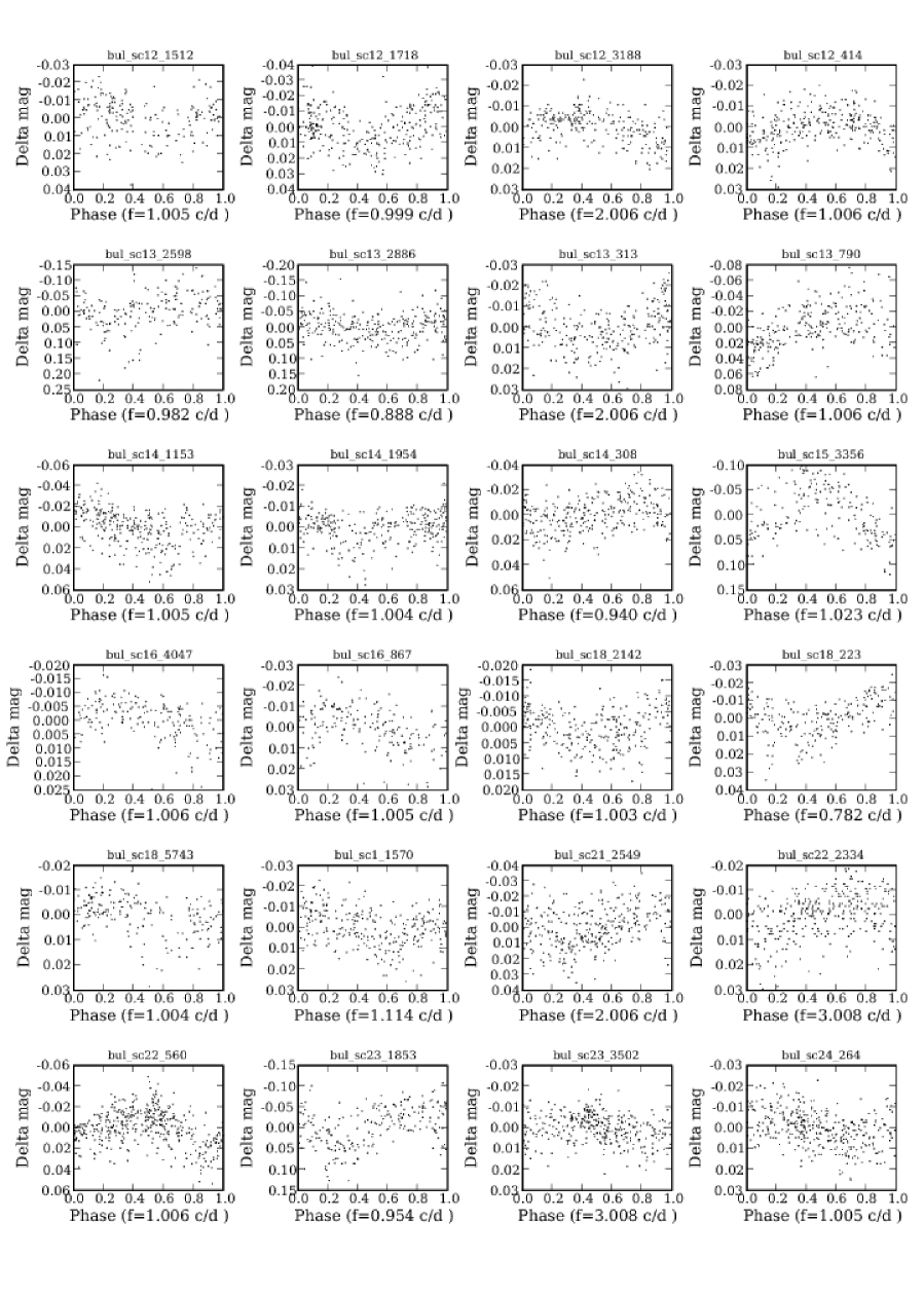
Figure 31: Phase plots of variables in the Galactic Bulge classified as GDOR with both the MSBN and the GM method, and not present in the list of Pigulski. The OGLE identifier is shown, and the dominant frequency, used to fold the light curves, in units of cycles per day (c/d).

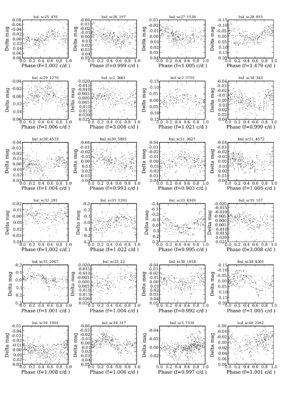
Figure 32: Phase plots of variables in the Galactic Bulge classified as GDOR with both the MSBN and the GM method, and not present in the list of Pigulski. The OGLE identifier is shown, and the dominant frequency, used to fold the light curves, in units of cycles per day (c/d).

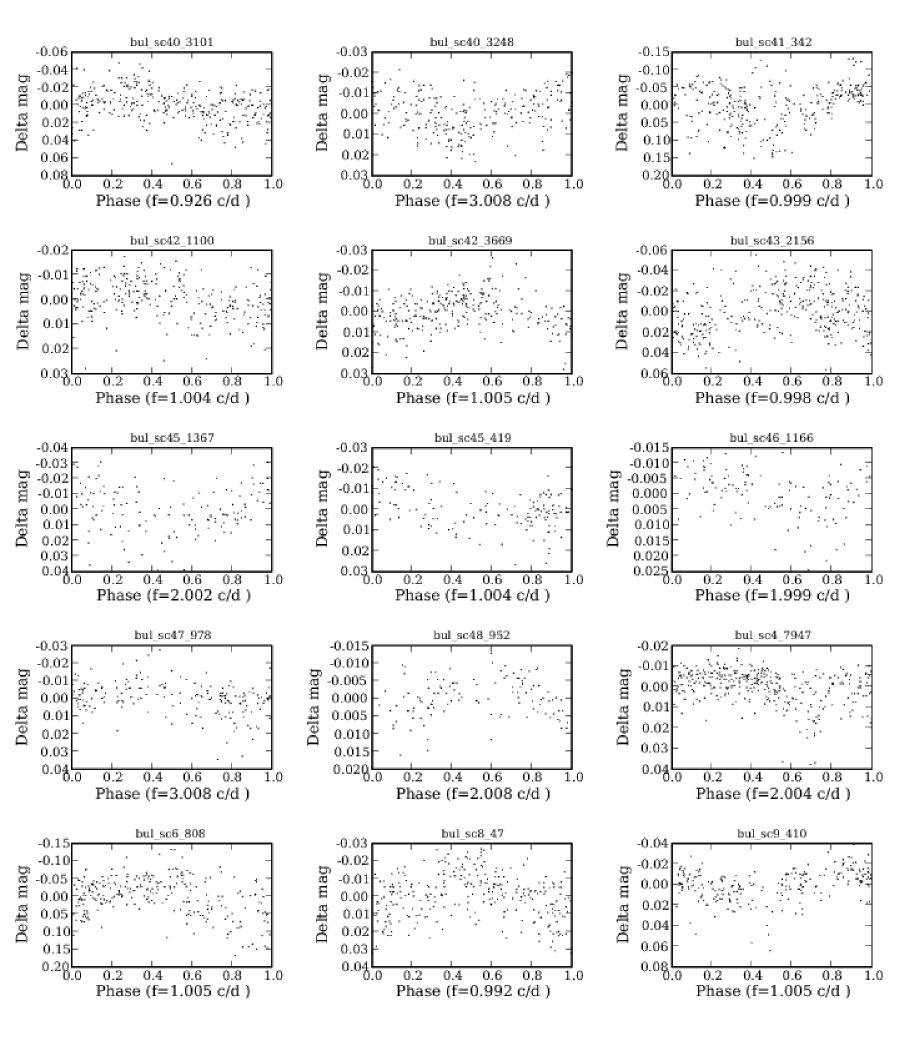
Figure 33: Phase plots of variables in the Galactic Bulge classified as GDOR with both the MSBN and the GM method, and not present in the list of Pigulski. The OGLE identifier is shown, and the dominant frequency, used to fold the light curves, in units of cycles per day (c/d).

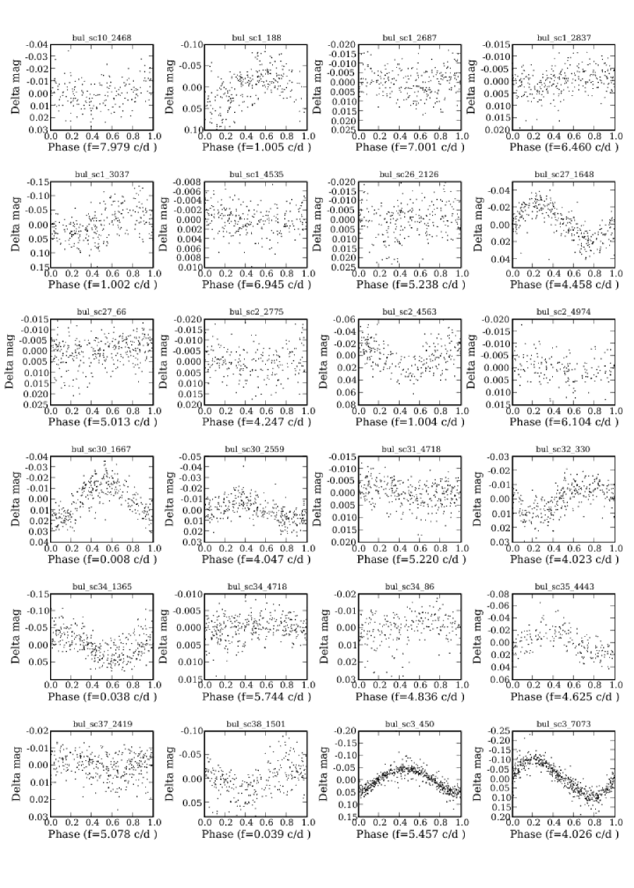
Figure 34: Phase plots of variables in the Galactic Bulge classified as BCEP with both the MSBN and the GM method, and not present in the list of Pigulski. The OGLE identifier is shown, and the dominant frequency, used to fold the light curves, in units of cycles per day (c/d).

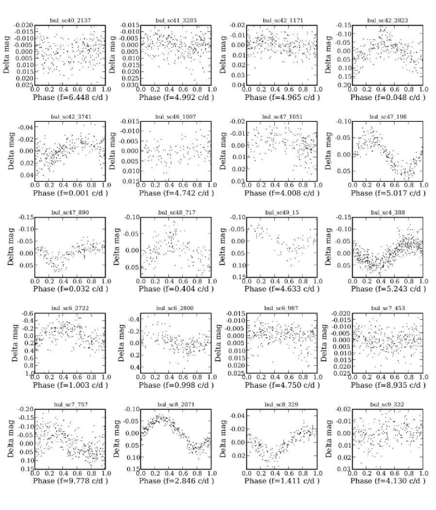
Figure 35: Phase plots of variables in the Galactic Bulge classified as BCEP with both the MSBN and the GM method, and not present in the list of Pigulski. The OGLE identifier is shown, and the dominant frequency, used to fold the light curves, in units of cycles per day (c/d).

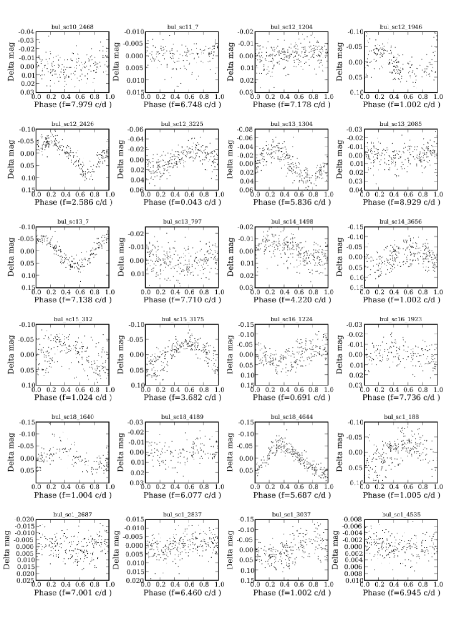
Figure 36: Phase plots of variables in the Galactic Bulge classified as DSCUT with both the MSBN and the GM method, and not present in the list of Pigulski. The OGLE identifier is shown, and the dominant frequency, used to fold the light curves, in units of cycles per day (c/d).

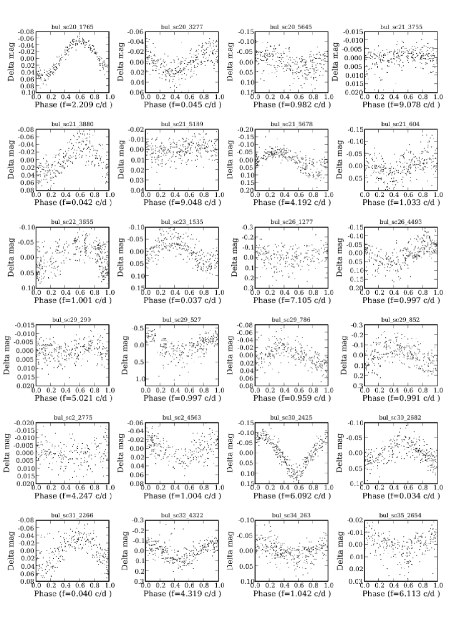
Figure 37: Phase plots of variables in the Galactic Bulge classified as DSCUT with both the MSBN and the GM method, and not present in the list of Pigulski. The OGLE identifier is shown, and the dominant frequency, used to fold the light curves, in units of cycles per day (c/d).

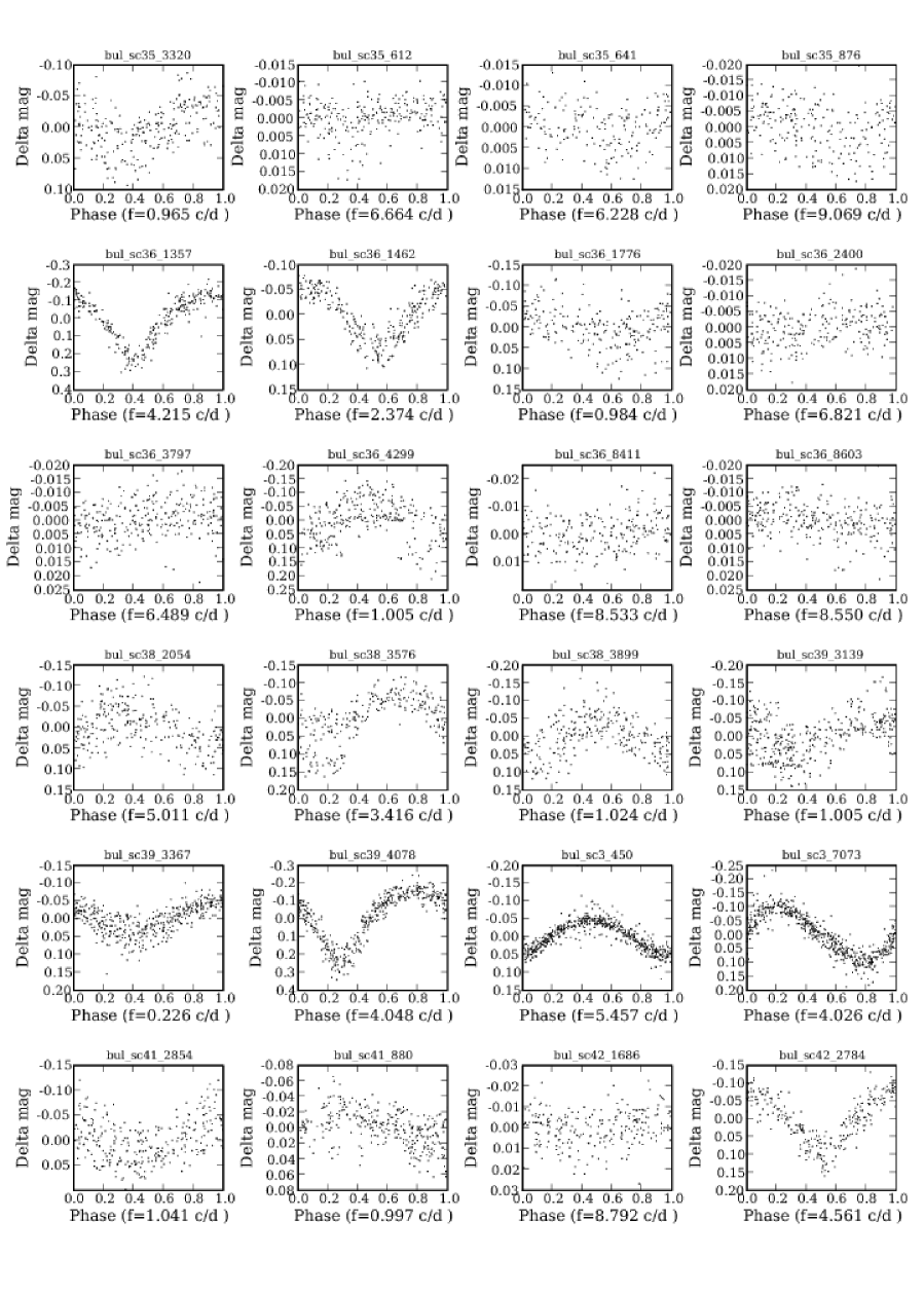
Figure 38: Phase plots of variables in the Galactic Bulge classified as DSCUT with both the MSBN and the GM method, and not present in the list of Pigulski. The OGLE identifier is shown, and the dominant frequency, used to fold the light curves, in units of cycles per day (c/d).

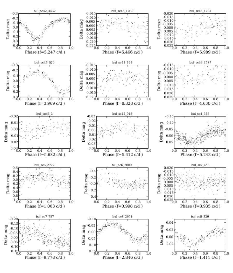
Figure 39: Phase plots of variables in the Galactic Bulge classified as DSCUT with both the MSBN and the GM method, and not present in the list of Pigulski. The OGLE identifier is shown, and the dominant frequency, used to fold the light curves, in units of cycles per day (c/d).

Table 15: Basic light curve and physical properties of Galactic Bulge stars classified as SPB with both the MSBN and the GM method. The dominant frequency $f_{1}$, the second frequency $f_{2}$ and the V-I colour index are listed. Several of these stars might be evolved pulsators, termed PVSG here, rather than SPB.

Object identifier	$f_{1}$ ($c/d$)	$f_{2}$ ($c/d$)	V-I (mag)
bul_sc11_1972	$1.530$	$1.768$	$-0.13$
bul_sc11_78	$2.006$	$3.852$	$-0.16$
bul_sc12_1585	$0.054$	$0.040$	$0.01$
bul_sc12_2793	$0.943$	$0.057$	$0.07$
bul_sc13_1232	$0.625$	$0.313$	$-0.03$
bul_sc14_2530	$0.997$	$2.005$	$-0.17$
bul_sc18_2633	$1.005$	$0.002$	$0.05$
bul_sc20_5489	$0.076$	$0.038$	$-0.01$
bul_sc22_2197	$1.008$	$1.028$	$-0.04$
bul_sc26_1513	$1.005$	$0.001$	$-0.15$
bul_sc29_1066	$0.019$	$0.001$	$-0.01$
bul_sc30_4914	$1.005$	$0.001$	$-0.06$
bul_sc32_1717	$2.910$	$7.858$	$-0.12$
bul_sc33_1385	$0.011$	$0.020$	$0.05$
bul_sc35_905	$1.006$	$0.980$	$-0.13$
bul_sc36_1523	$0.052$	$0.052$	$-0.13$
bul_sc36_1648	$0.004$	$0.001$	$0.07$
bul_sc36_6405	$0.054$	$0.056$	$0.03$
bul_sc37_3960	$0.999$	$0.002$	$-0.01$
bul_sc39_700	$0.028$	$0.003$	$-0.02$
bul_sc40_897	$1.007$	$1.005$	$0.04$
bul_sc42_1528	$1.005$	$1.044$	$0.08$
bul_sc42_3374	$1.004$	$0.997$	$-0.03$
bul_sc42_3470	$0.998$	$1.999$	$-0.13$

Table 16: Basic light curve and physical properties of Galactic Bulge stars classified as GDOR with both the MSBN and the GM method. The dominant frequency $f_{1}$, the second frequency $f_{2}$ and the V-I colour index are listed.

Object identifier	$f_{1}$ ($c/d$)	$f_{2}$ ($c/d$)	V-I (mag)
bul_sc1_1570	$1.114$	$0.103$	$0.41$
bul_sc2_3661	$3.008$	$7.808$	$0.39$
bul_sc2_3755	$1.021$	$0.003$	$0.47$
bul_sc3_7330	$0.997$	$0.470$	$0.35$
bul_sc4_7947	$2.004$	$0.011$	$0.53$
bul_sc6_808	$1.005$	$0.020$	$0.50$
bul_sc8_47	$0.992$	$0.005$	$0.49$
bul_sc9_410	$1.005$	$0.065$	$0.40$
bul_sc12_1512	$1.005$	$2.089$	$0.49$
bul_sc12_1718	$0.999$	$1.006$	$0.42$
bul_sc12_3188	$2.006$	$0.542$	$0.42$
bul_sc12_414	$1.006$	$2.005$	$0.43$
bul_sc13_2598	$0.982$	$2.004$	$0.46$
bul_sc13_2886	$0.888$	$6.009$	$0.54$
bul_sc13_313	$2.006$	$1.002$	$0.47$
bul_sc13_790	$1.006$	$0.009$	$0.53$
bul_sc14_1153	$1.005$	$0.998$	$0.32$
bul_sc14_308	$0.940$	$1.005$	$0.53$
bul_sc14_1954	$1.004$	$3.673$	$0.50$
bul_sc15_3356	$1.023$	$1.006$	$0.36$
bul_sc16_867	$1.005$	$5.711$	$0.54$
bul_sc16_4047	$1.006$	$7.194$	$0.46$
bul_sc18_2142	$1.003$	$3.008$	$0.51$
bul_sc18_223	$0.782$	$0.784$	$0.54$
bul_sc18_5743	$1.004$	$6.058$	$0.48$
bul_sc21_2549	$2.006$	$0.043$	$0.52$
bul_sc22_2334	$3.008$	$0.999$	$0.52$
bul_sc22_560	$1.006$	$0.050$	$0.46$
bul_sc23_3502	$3.008$	$0.001$	$0.46$
bul_sc23_1853	$0.954$	$0.048$	$0.49$
bul_sc24_264	$1.005$	$8.774$	$0.47$
bul_sc25_476	$1.002$	$0.988$	$0.32$
bul_sc26_197	$0.999$	$0.948$	$0.47$
bul_sc27_1538	$1.005$	$0.096$	$0.44$
bul_sc28_855	$1.479$	$1.480$	$0.33$
bul_sc29_1270	$1.006$	$0.007$	$0.46$
bul_sc30_343	$0.999$	$0.193$	$0.38$
bul_sc30_4533	$1.004$	$3.971$	$0.35$
bul_sc30_5895	$0.993$	$0.066$	$0.54$
bul_sc31_3627	$0.903$	$0.075$	$0.34$
bul_sc31_4572	$1.005$	$0.055$	$0.50$
bul_sc32_281	$1.002$	$2.394$	$0.53$
bul_sc33_1203	$1.022$	$0.032$	$0.45$
bul_sc33_4349	$0.995$	$1.011$	$0.34$
bul_sc35_107	$3.008$	$7.215$	$0.50$
bul_sc35_2067	$1.001$	$1.005$	$0.45$
bul_sc35_22	$1.004$	$4.042$	$0.41$
bul_sc38_1818	$0.992$	$4.913$	$0.51$
bul_sc38_4301	$1.005$	$0.990$	$0.41$
bul_sc39_1901	$1.008$	$1.003$	$0.42$
bul_sc39_317	$1.006$	$1.007$	$0.45$
bul_sc40_2162	$1.001$	$0.019$	$0.42$
bul_sc40_3101	$0.926$	$0.061$	$0.47$
bul_sc40_3248	$3.008$	$9.208$	$0.43$
bul_sc41_342	$0.999$	$0.011$	$0.53$
bul_sc42_1100	$1.004$	$1.006$	$0.51$
bul_sc42_3669	$1.005$	$8.812$	$0.43$
bul_sc43_2156	$0.998$	$0.032$	$0.36$
bul_sc45_1367	$2.002$	$6.468$	$0.43$
bul_sc45_419	$1.004$	$5.367$	$0.41$
bul_sc46_1166	$1.999$	$6.525$	$0.44$
bul_sc47_978	$3.008$	$0.840$	$0.46$
bul_sc48_952	$2.008$	$7.209$	$0.46$

Table 17: Basic light curve and physical properties of Galactic Bulge stars classified as BCEP with both the MSBN and the GM method. The dominant frequency $f_{1}$, the second frequency $f_{2}$ and the V-I colour index are listed. Several of these stars might be evolved pulsators, termed PVSG here, rather than BCEP.

Object identifier	$f_{1}$ ($c/d$)	$f_{2}$ ($c/d$)	V-I (mag)
bul_sc1_4535	$6.945$	$6.122$	$0.39$
bul_sc1_2687	$7.001$	$5.029$	$0.40$
bul_sc1_2837	$6.460$	$1.006$	$0.44$
bul_sc1_3037	$1.002$	$0.022$	$0.49$
bul_sc1_188	$1.005$	$0.976$	$0.27$
bul_sc2_2775	$4.247$	$8.952$	$0.41$
bul_sc2_4563	$1.004$	$0.491$	$0.35$
bul_sc2_4974	$6.104$	$7.784$	$0.46$
bul_sc3_450	$5.457$	$0.440$	$0.45$
bul_sc3_7073	$4.026$	$0.438$	$0.45$
bul_sc4_388	$5.243$	$2.621$	$0.51$
bul_sc6_2722	$1.003$	$0.005$	$0.29$
bul_sc6_2800	$0.998$	$1.004$	$0.33$
bul_sc6_987	$4.750$	$8.153$	$0.47$
bul_sc7_757	$9.778$	$7.772$	$0.31$
bul_sc7_453	$8.935$	$6.939$	$0.52$
bul_sc8_2071	$2.846$	$3.972$	$0.41$
bul_sc8_329	$1.411$	$1.003$	$0.41$
bul_sc9_332	$4.130$	$2.854$	$0.54$
bul_sc10_2468	$7.979$	$8.872$	$0.42$
bul_sc26_2126	$5.238$	$8.780$	$-0.28$
bul_sc27_1648	$4.458$	$0.553$	$-0.16$
bul_sc27_66	$5.013$	$6.710$	$-0.16$
bul_sc30_1667	$0.008$	$1.002$	$-0.19$
bul_sc30_2559	$4.047$	$1.003$	$-0.03$
bul_sc31_4718	$5.220$	$9.492$	$-0.18$
bul_sc32_330	$4.023$	$0.004$	$0.17$
bul_sc34_1365	$0.038$	$0.003$	$-0.17$
bul_sc34_4718	$5.744$	$1.404$	$-0.19$
bul_sc34_86	$4.836$	$0.005$	$-0.14$
bul_sc35_4443	$4.625$	$0.003$	$-0.11$
bul_sc37_2419	$5.078$	$1.005$	$-0.24$
bul_sc38_1501	$0.039$	$1.041$	$-0.30$
bul_sc40_2137	$6.448$	$8.439$	$-0.14$
bul_sc41_3203	$4.992$	$1.001$	$-0.13$
bul_sc42_1171	$4.965$	$1.224$	$-0.26$
bul_sc42_2823	$0.048$	$0.049$	$-0.29$
bul_sc42_3741	$0.001$	$0.003$	$-0.36$
bul_sc46_1007	$4.742$	$5.299$	$-0.18$
bul_sc47_1051	$4.008$	$0.998$	$-0.34$
bul_sc47_198	$5.017$	$4.016$	$-0.29$
bul_sc47_890	$0.032$	$0.031$	$-0.21$
bul_sc48_717	$0.404$	$0.001$	$-0.26$
bul_sc49_15	$4.633$	$2.316$	$0.07$

Table 18: Basic light curve and physical properties of Galactic Bulge stars classified as DSCUT with both the MSBN and the GM method. The dominant frequency $f_{1}$, the second frequency $f_{2}$ and the V-I colour index are listed.

Object identifier	$f_{1}$ ($c/d$)	$f_{2}$ ($c/d$)	V-I (mag)
bul_sc1_4535	$6.945$	$6.122$	$0.39$
bul_sc1_2687	$7.001$	$5.029$	$0.40$
bul_sc1_2837	$6.460$	$1.006$	$0.44$
bul_sc1_3037	$1.002$	$0.022$	$0.49$
bul_sc1_188	$1.005$	$0.976$	$0.27$
bul_sc2_2775	$4.247$	$8.952$	$0.41$
bul_sc2_4563	$1.004$	$0.491$	$0.35$
bul_sc3_450	$5.457$	$0.440$	$0.45$
bul_sc3_7073	$4.026$	$0.438$	$0.45$
bul_sc4_388	$5.243$	$2.621$	$0.51$
bul_sc6_2722	$1.003$	$0.005$	$0.29$
bul_sc6_2800	$0.998$	$1.004$	$0.33$
bul_sc7_757	$9.778$	$7.772$	$0.31$
bul_sc7_453	$8.935$	$6.939$	$0.52$
bul_sc8_2071	$2.846$	$3.972$	$0.41$
bul_sc8_329	$1.411$	$1.003$	$0.41$
bul_sc9_332	$4.130$	$2.854$	$0.54$
bul_sc10_2468	$7.979$	$8.872$	$0.42$
bul_sc11_7	$6.748$	$2.538$	$0.44$
bul_sc12_1946	$1.002$	$0.085$	$0.23$
bul_sc12_3225	$0.043$	$0.048$	$0.52$
bul_sc12_1204	$7.178$	$1.004$	$0.47$
bul_sc12_2426	$2.586$	$1.353$	$0.50$
bul_sc13_2085	$8.929$	$9.719$	$0.45$
bul_sc13_797	$7.710$	$9.461$	$0.37$
bul_sc13_7	$7.138$	$0.001$	$0.53$
bul_sc13_1304	$5.836$	$0.001$	$0.70$
bul_sc14_1498	$4.220$	$2.932$	$0.34$
bul_sc14_3656	$1.002$	$0.023$	$0.36$
bul_sc15_312	$1.024$	$0.004$	$0.45$
bul_sc15_3175	$3.682$	$1.841$	$0.23$
bul_sc16_1224	$0.691$	$0.345$	$0.16$
bul_sc16_1923	$7.736$	$0.255$	$0.53$
bul_sc18_1640	$1.004$	$0.992$	$0.35$
bul_sc18_4189	$6.077$	$4.922$	$0.51$
bul_sc18_4644	$5.687$	$9.645$	$0.49$
bul_sc20_1765	$2.209$	$1.006$	$0.45$
bul_sc20_3277	$0.045$	$1.028$	$0.38$
bul_sc20_5645	$0.982$	$0.029$	$0.49$
bul_sc21_3755	$9.078$	$8.027$	$0.51$
bul_sc21_3880	$0.042$	$0.971$	$0.40$
bul_sc21_5678	$4.192$	$2.096$	$0.38$
bul_sc21_5189	$9.048$	$7.945$	$0.54$
bul_sc21_604	$1.033$	$0.004$	$0.35$
bul_sc22_3655	$1.001$	$0.038$	$0.37$
bul_sc23_1535	$0.037$	$0.028$	$0.40$
bul_sc26_1277	$7.105$	$8.102$	$0.46$
bul_sc26_4493	$0.997$	$0.019$	$0.24$
bul_sc29_299	$5.021$	$9.005$	$0.47$
bul_sc29_527	$0.997$	$0.001$	$0.14$
bul_sc29_786	$0.959$	$1.958$	$0.40$
bul_sc29_852	$0.991$	$1.001$	$0.26$
bul_sc30_2425	$6.092$	$3.046$	$0.42$
bul_sc30_2682	$0.034$	$0.017$	$0.37$
bul_sc31_2266	$0.040$	$0.020$	$0.48$
bul_sc32_4322	$4.319$	$0.008$	$0.31$
bul_sc34_263	$1.042$	$0.029$	$0.20$
bul_sc35_2654	$6.113$	$0.001$	$0.52$
bul_sc35_3320	$0.965$	$1.001$	$0.27$
bul_sc35_612	$6.664$	$4.674$	$0.46$
bul_sc35_641	$6.228$	$8.510$	$0.42$
bul_sc35_876	$9.069$	$8.432$	$0.43$

Table 19: Basic light curve and physical properties of Galactic Bulge stars classified as DSCUT with both the MSBN and the GM method (continued). The dominant frequency $f_{1}$, the second frequency $f_{2}$ and the V-I colour index are listed.

Object identifier	$f_{1}$ ($c/d$)	$f_{2}$ ($c/d$)	V-I (mag)
bul_sc36_1462	$2.374$	$1.187$	$0.42$
bul_sc36_1357	$4.215$	$7.326$	$0.51$
bul_sc36_1776	$0.984$	$0.004$	$0.48$
bul_sc36_2400	$6.821$	$6.853$	$0.50$
bul_sc36_3797	$6.489$	$5.983$	$0.35$
bul_sc36_4299	$1.005$	$0.999$	$0.53$
bul_sc36_8411	$8.533$	$1.673$	$0.50$
bul_sc36_8603	$8.550$	$5.868$	$0.49$
bul_sc38_2054	$5.011$	$5.162$	$0.47$
bul_sc38_3576	$3.416$	$1.708$	$0.43$
bul_sc38_3899	$1.024$	$0.001$	$0.18$
bul_sc39_3139	$1.005$	$0.016$	$0.22$
bul_sc39_3367	$0.226$	$0.113$	$0.40$
bul_sc39_4078	$4.048$	$1.003$	$0.49$
bul_sc41_2854	$1.041$	$0.040$	$0.46$
bul_sc41_880	$0.997$	$1.026$	$0.51$
bul_sc42_1686	$8.792$	$5.969$	$0.51$
bul_sc42_2784	$4.561$	$5.920$	$0.46$
bul_sc42_3467	$5.247$	$0.001$	$0.17$
bul_sc45_1032	$6.466$	$7.232$	$0.44$
bul_sc45_1703	$5.989$	$4.237$	$0.53$
bul_sc45_520	$3.969$	$3.687$	$0.23$
bul_sc45_595	$8.328$	$1.674$	$0.38$
bul_sc46_1787	$4.630$	$9.715$	$0.48$
bul_sc46_3	$5.682$	$0.476$	$0.48$
bul_sc46_918	$5.412$	$6.028$	$0.41$