Charge instabilities and electron-phonon interaction in the Hubbard-Holstein model

Abstract

We consider the Hubbard-Holstein model in the adiabatic limit to investigate the effects of electron-electron interactions on the electron-phonon coupling. To this aim we compute at any momentum and filling the static charge susceptibility of the Hubbard model within the Gutzwiller approximation and we find that electron-electron correlations effectively screen the electron coupling to the lattice. This screening is more effective at large momenta and, as a consequence, the charge-density wave phase due to the usual Peierls instability of the Fermi surface momenta is replaced by a phase-separation instability when the correlations are sizable.

I Introduction

In the last years the issue of electron-phonon ($e$-$ph$) coupling in the presence of strong electron-electron ($e$-$e$) correlations has been raised in a variety of contexts. For instance, in the high-temperature superconducting cuprates recent photoemission experimentsLan01 ; DAs02 ; Gwe04 indicate a sizable coupling of electrons with collective modes, possibly of phononic nature, while the softening of a phonon peak in inelastic neutron scattering experiments, Rez06 ; Rez07 as well as features in tunnelling spectralee06 suggest that electrons are substantially coupled to the lattice in these materials. At the same time optical and transport experiments do not display a strong $e$-$ph$ coupling except at very small doping, where polaronic features have been observed. polaronexper1 ; polaronexper2 ; polaronexper3 An intriguing interplay between lattice and electrons has also been invoked to explain transport in manganitesMil96 , in single-molecule junctionsGrempel and in fullerenes, Gun97 where a correlation-enhanced superconductivity has also been proposed. capone These examples show that the issue of $e$-$ph$ coupling in the presence of strong $e$-$e$ correlation is generally relevant and it translates in several related issues. First of all, the fact that various physical quantities appear to be differently affected by phonons indicates that the energy and momentum structure of the $e$-$ph$ coupling is important. In turn this emphasizes the role of $e$-$e$ interactions as an effective mechanism to induce strong energy and momentum dependencies in the $e$-$ph$ coupling. Secondly, phonons may be responsible for charge instabilities. One possibility is that they mediate interactions between electrons on the Fermi surface giving rise to charge-density waves or Peierls distortions. It has also been proposedGri94 ; CDCG95 that a phonon-induced attraction gives rise to an electronic phase separation (although in real systems this is ultimately prevented by the long-ranged Coulombic forces with the formation of nano- or mesoscopic domains, the so-called frustrated phase separation. low94 ; lor01I ; lor01II ; lor02 ; Ort06 ; Ort07 ; ort08 )

Due to the above, phonons coupled to strongly correlated electrons have already been investigated by means of numerical techniques like quantum Monte Carlo, HS83 ; hir83 ; HS84 ; Hir85 ; Ber95 ; Hua03 exact diagonalization, dob94 ; dob94epl ; lor94b ; stephan Dynamical Mean Field Theory (DMFT),  FJ95 ; Capo04 ; Kol04-1 ; Kol04-2 ; Jeo04 ; San05 ; San06 and (semi)analytical approaches like slave bosons (SB) and large-N expansions.  Gri94 ; Kel95 ; Zey96 ; Koc04 ; Cap04 ; Cit01 ; Cit05 Despite this variety of approaches, a systematic and thorough investigation within the same technical framework is not yet available either due to the demanding character of the numerical approaches or to the limited parameter ranges investigated so far. Therefore in this paper we study the renormalization of the electron-lattice coupling in the presence of strong $e$-$e$ correlations systematically considering the momentum, doping, and interaction-strength dependencies. In particular we want to elucidate how charge density wave (CDW) or phase separation (PS) instabilities are modified in the presence of $e$-$e$ interactions. To this aim we need a technique which is not numerically very demanding, but still provides a quantitatively acceptable treatment of the strongly correlated regime. In this regard we find the Gutzwiller approach and the related Gutzwiller Approximationgut63 (GA) a good compromise allowing extensive and systematic exploration of various parameter ranges while keeping a reliable treatment of the low-energy physics. It has recently been shown that the Gutzwiller variational approach provides remarkably accurate positions of complex magnetic phase boundaries in infinite dimensions. gun07 This indicates that the Gutzwiller energy and its derivatives are quite accurate. In this work we extend these results to the charge channel also in infinite dimensions, where the GA to the Gutzwiller variational problem is exact. met88 ; geb90 In addition, in order to make contact with layered systems, we study the two-dimensional (2d) case where the GA is still expected to give an accurate estimate of the energy. This also gives us the opportunity to study the interplay between nesting in the presence of electron phonon coupling, which favors Peierls distortions, and strong correlation which favors phase separation.

To obtain the phase diagram in the presence of both $e$-$e$ and $e$-$ph$ interactions, in principle, one should compute the GA energy for every possible charge-ordered state. However, it is much more practical to study the static response functions of the uniform state to an external perturbation and to locate the relevant instabilities. We show below that for Holstein phonons in the adiabatic limit, the exact charge susceptibility in the presence of $e$-$ph$ and $e$-$e$ interaction is simply related to the charge susceptibility without phonons. Therefore our work reduces to compute the latter which is done in the GA. This corresponds to the static limit of the GA+(random phase approximation), (GA+RPA), which was derived in Ref. sei01, and is rooted in Vollhardt’s Fermi liquid approach. vol84 As a byproduct our work generalizes Vollhardt’s computation of the zero-momentum and half-filled charge susceptibility to any momentum and filling. Our approach is not as accurate as QMC or DMFT studies as far as the electron dynamical excitations are concerned, because it inherently deals with the quasiparticle part of their spectrum. Nonetheless with relatively small numerical efforts it allows for a systematic analysis of momentum, doping and interaction dependencies of the screening processes underlying the quasiparticle charge response and the related $e$-$ph$ coupling.

It is worth mentioning that the dynamical version of our GA+RPA approach has been tested in various situations and found to be accurate compared with exact diagonalization. sei01 ; sei03 ; sei04b ; sei07b Computations for realistic models have provided a description of different physical quantities in accord with experiment. lor02b ; lor03 ; sei05 The present analysis of the charge susceptibility of the paramagnetic state gives us an opportunity to present the method in a simpler context with respect to the more complex situations considered in the past, thus allowing for the clarification of several methodological aspects. On the other hand, restricting to the paramagnetic state we ignore antiferromagnetic and related instabilities that arise as the system approaches half-filling.

The scheme of our paper is as follows. We first present in Sect. II the derivation of an exact result for the renormalization of the $e$-$ph$ coupling in the adiabatic limit. The GA+RPA approach is presented in Sect. III and then it is exploited to systematically calculate the momentum, doping, and interaction dependencies of the charge susceptibility of the Hubbard model. The results in $d=\infty$ are contained in Sect. IV, while the 2d case is reported in Sect. V. Our conclusions can be found in Sect. VI, while the details of our calculations are given in the Appendix.

II Exact relation between electron-phonon instabilities and charge susceptibility

In this section we show the renormalization of the $e$-$ph$ coupling and how the renormalized coupling is related to the electronic susceptibility. We consider a single band system with $e$-$e$ interaction and $e$-$ph$ coupling on a lattice

$$H_{tot}=H_{e}+H_{eph}+H_{ph}$$ (1)

Specifically we consider the Holstein interaction

$$H_{eph}+H_{ph}=\sum_{i}\beta x_{i}(\hat{n}_{i}-n)+\sum_{i}\left(\frac{P_{i}^{2}}{2M}+\frac{1}{2}Kx_{i}^{2}\right)$$ (2)

where $\hat{n}_{i}$ is the electronic density operator; $n=N_{p}/N$ is the average density on a lattice with $N$ sites and $N_{p}$ particles. $P_{i}$, $x_{i}$ and $M$ are the momentum, the displacement and the mass of the lattice ions respectively. We treat Eq. (2) in the extreme adiabatic limit ($M$$\rightarrow$$\infty$), where, using the Born-Oppenheimer’s principle, we can represent the ground state of the system as $|\psi_{tot}\rangle=|\psi_{e}\rangle|\chi_{ph}\rangle$. The electronic wave function $|\psi_{e}\rangle$ depends parametrically on the ionic displacement $x_{i}$. We assume that the ground state in the absence of $e$-$ph$ coupling is uniform [i.e., no static CDW state is present]. For a fixed configuration of displacements $\{x_{i}\}$, the $e$-$ph$ term of Eq. (2) acts as an external field on the electrons, producing a density deviation $\{\delta n_{i}\}$, being $\delta n_{i}=\langle\hat{n}_{i}\rangle-n$.

The total energy in the adiabatic limit has the form

$$E_{tot}=E_{e}[\delta n]+E_{eph}[\delta n,x]+E_{ph}[x]$$ (3)

where $E_{e}=\langle\psi_{tot}|H_{e}|\psi_{tot}\rangle$, $E_{eph}=\langle\psi_{tot}|H_{eph}|\psi_{tot}\rangle$ and $E_{ph}=\langle\psi_{tot}|H_{ph}|\psi_{tot}\rangle$, and $\delta n$, $x$ stand for the sets $\{\delta n_{i}\}$ and $\{x_{i}\}$ respectively. We move to momentum space and perform an expansion of $E_{e}[\delta n]$ up to the second order in the density deviation $\delta n$

$$E_{e}[\delta n]=E_{e}^{(0)}+\sum_{{\bf q}}\left(\frac{\partial E_{e}}{\partial n_{{\bf q}}}\right)_{0}\delta n_{{\bf q}}+\frac{1}{2}\sum_{{\bf q}}\left(\frac{\partial^{2}E_{e}}{\partial n_{{\bf q}}\partial n_{-{\bf q}}}\right)_{0}\delta n_{{\bf q}}\delta n_{-{\bf q}},$$ (4)

where the label “$0$” indicates that the derivatives must be evaluated within the uniform electronic state (in the absence of the $e$-$ph$ coupling); $E_{e}^{(0)}$ is therefore the ground state energy in the absence of the $e$-$ph$ coupling. The first order term vanishes identically. For the ${\bf q}\neq 0$ terms this arises because stability requires that odd powers in the $\delta n_{\bf q}$ expansion must vanish (otherwise the systems would lower its energy by creating a CDW state). Instead the ${\bf q}=0$ term with $\partial E_{e}/\partial n_{{\bf q}=0}$ vanishes because we are working at a fixed particle number ($\delta n_{{\bf q}=0}=0$). Therefore the electronic ground state energy is quadratic in the density deviation

$$E_{e}[\delta n_{i}]=E_{e}^{(0)}+\frac{1}{2}\sum_{{\bf q}}\kappa^{-1}_{{\bf q}}\delta n_{{\bf q}}\delta n_{-{\bf q}}$$ (5)

where we customarily define $\kappa_{{\bf q}}^{-1}\equiv\left(\frac{\partial^{2}E_{e}}{\partial\delta n_{{\bf q}}^{2}}\right)_{0}$ with $\kappa_{{\bf q}}$ being the static charge susceptibility of the electronic system in the absence of the $e$-$ph$ coupling.

We now minimize the Holstein energy

$$E_{H}=E_{eph}[\delta n,x]+E_{ph}[x]=\sum_{i}\left(\beta x_{i}\delta n_{i}+\frac{1}{2}Kx_{i}^{2}\right)$$ (6)

with respect to the ionic displacements $x_{i}$ at fixed $\delta n_{i}$ finding $x_{i}$=$-\beta\delta n_{i}/K$. Replacing this expression in Eq. (6) and introducing the adimensional coupling

$$\lambda\equiv\frac{\chi^{0}_{0}\beta^{2}}{K}$$ (7)

[$\chi^{0}_{0}$ is the density of states (DOS) of the non interacting electron system], we find the following expression for $E_{tot}$

$$E_{tot}=E^{(0)}_{tot}+\frac{1}{2}\sum_{{\bf q}}\left(\kappa^{eph}_{{\bf q}}\right)^{-1}\delta n_{{\bf q}}\delta n_{-{\bf q}}$$ (8)

with

$$\kappa^{eph}_{{\bf q}}=\frac{\kappa_{\bf q}}{1-\lambda\kappa_{\bf q}/\chi^{0}_{0}}=\frac{\kappa_{\bf q}}{1-\tilde{\lambda}_{\bf q}}$$ (9)

where we introduced the renormalized coupling

$$\tilde{\lambda}_{\bf q}\equiv\frac{\lambda\kappa_{\bf q}}{\chi^{0}_{0}}.$$ (10)

Eqs. (8)-(10) provide the exact second-order expansion of the total energy in the adiabatic limit and establish a relation between the electronic charge susceptibilities, $\kappa_{{\bf q}}$ and $\kappa^{eph}_{{\bf q}}$, in the absence and in the presence of the $e$-$ph$ coupling respectively. By construction $\tilde{\lambda}_{\bf q}$ is defined in such a way that $\tilde{\lambda}_{\bf q}=1$ indicates an instability, in analogy with the noninteracting $e$-$ph$ coupling for which $\lambda=1$ indicates a ${\bf q}=0$ instability.

We can write $\tilde{\lambda}_{\bf q}=\beta\Gamma_{\bf q}\kappa^{0}_{\bf q}/K$, using the charge vertexKel95 ; Hua03 ; Koc04 ; Cap04 ; Cit01 ; Cit05 which acts as a renormalized quasiparticle-$ph$ coupling

$$\Gamma_{\bf q}\equiv\frac{\kappa_{\bf q}}{\kappa^{0}_{\bf q}}\beta$$ (11)

($\kappa^{0}_{\bf q}$ is the non interacting susceptibility). Then we find

$$\frac{\tilde{\lambda}_{\bf q}}{\lambda}=\frac{\kappa^{0}_{\bf q}}{\chi^{0}_{0}}\frac{\Gamma_{\bf q}}{\beta}$$ (12)

Eq. (12) has been introduced to separate in the $e$-$ph$ coupling the effects of finite ${\bf q}$ from those of the $e$-$e$ renormalization. Specifically, $\kappa^{0}_{\bf q}/\chi^{0}_{0}$ contains the effects of finite momentum, and is present even for non-interacting electrons, while the $e$-$e$ interaction acts on the $e$-$ph$ coupling via a modification of the electronic charge susceptibility, given by $\Gamma_{\bf q}/\beta$. In this exact adiabatic derivation both these effects act in a simple multiplicative manner on $\lambda$.

A second feature of the result in Eq. (9) is that the system can become unstable if, upon increasing $\lambda$, it meets the condition $\lambda=\lambda_{c}$ with

$$\lambda=\lambda_{c}=\chi^{0}_{0}/\kappa_{{\bf q}_{c}}$$ (13)

for some ${\bf q}_{c}$. In this case, if no other (first-order) instabilities take place before, the system undergoes a transition to a charge-ordered state with a typical wavevector ${\bf q}_{c}$.

Now the whole issue to study the effects of $e$-$e$ interactions on the $e$-$ph$ coupling and the related electronic charge instability is reduced to the study of the electronic charge susceptibility (in the absence of the $e$-$ph$ interaction). This is the main goal of the subsequent sections.

III Formalism

In order to compute the static charge susceptibility, we evaluate the electronic energy in the presence of an external field $f$

$$H_{f}=\sum_{ij\sigma}f_{ij\sigma}c^{{\dagger}}_{i\sigma}c_{j\sigma}$$ (14)

where $c^{{\dagger}}_{i\sigma}$($c_{i\sigma}$) are creation (annihilation) fermionic operators and $f_{ij}=f^{*}_{ji}$.

Insofar our treatment of the $e$-$e$ interactions has been general. Starting from this section, we will adopt the one-band Hubbard model with hopping $t_{ij}$ extended to whatever neighbors $i$,$j$

$$H_{e}=\sum_{ij\sigma}t_{ij}c^{{\dagger}}_{i\sigma}c_{j\sigma}+\sum_{i}U\hat{n}_{i\uparrow}\hat{n}_{i\downarrow}$$ (15)

$\hat{n}_{i\sigma}$=$c^{{\dagger}}_{i\sigma}c_{i\sigma}$ is the density operator associated to the operators $c^{{\dagger}}_{i\sigma}$, $c_{i\sigma}$ and $U$ is the on-site Hubbard repulsion. In the numerical computations below we consider only nearest neighbor hopping $t_{ij}=-t$ to be nonzero.

We apply the Gutzwiller (GZW) variational method to Eq. (15) on d-dimensional hypercubic lattices with lattice parameter $a$=1. We consider the GZW ansatz state $|\psi\rangle=\hat{P}|Sd\rangle$, where the GZW projectorgeb90 $\hat{P}$ acts on the Slater determinant $|Sd\rangle$. Although we analyze a paramagnetic uniform state in order to determine the stability we need the energy in the presence of an arbitrary perturbation of the charge thus $|Sd\rangle$ shall allow for broken symmetries.

The GZW variational problem can not be solved exactly except for particular cases, as for $d$=$\infty$. Thus one uses the GA. In particular, we use the energy functional $E_{e}[\rho,D]$ obtained by Gebhardgeb90 which is equivalent to the Kotliar-Ruckenstein saddle point energy Kot86

$$E_{e}[\rho,D]=\sum_{ij\sigma}t_{ij}z_{i\sigma}z_{j\sigma}\rho_{ji\sigma}+\sum_{i}UD_{i}$$ (16)

with the GA hopping factors $z_{i\sigma}$

$$z_{i\sigma}[\rho,D]=\frac{\sqrt{(1-\rho_{ii}+D_{i})(\rho_{ii\sigma}-D_{i})}+\sqrt{D_{i}(\rho_{ii,-\sigma}-D_{i})}}{\sqrt{\rho_{ii\sigma}(1-\rho_{ii\sigma})}}$$ (17)

being $\rho_{ii}$=$\sum_{\sigma}\rho_{ii\sigma}$. Here $\rho$ is the single fermion density matrix in the uncorrelated state $\rho_{ji\sigma\sigma^{{}^{\prime}}}=\langle Sd|c^{{\dagger}}_{i\sigma}c_{j\sigma^{{}^{\prime}}}|Sd\rangle$. $D$ is the vector of the GA double occupancy parameters $D_{i}=\langle\psi|\hat{n}_{i\uparrow}\hat{n}_{i\downarrow}|\psi\rangle$.

To consider arbitrary deviations, the charge and spin distribution $\rho$ and the set of $D$ should be completely unrestricted. Since we will consider essentially charge deviations only the part diagonal in the spin indexes contributes, therefore we will use the notation $\rho_{ij\sigma}\equiv\rho_{ij\sigma\sigma}$.

One can show that the expectation value of the diagonal elements $\rho_{ii\sigma}$, calculated for the $|Sd\rangle$, coincides with the value of the density $n_{i\sigma}$, calculated for the GZW state $|\psi\rangle$.geb90 Namely,

$$n_{i\sigma}=\langle\psi|{c}^{{\dagger}}_{i\sigma}c_{i\sigma}|\psi\rangle=\rho_{ii\sigma}=\langle Sd|{c}^{{\dagger}}_{i\sigma}c_{i\sigma}|Sd\rangle$$ (18)

Eq. (18) will permit us to express charge density deviations $\delta n_{i}=\sum_{\sigma}\delta n_{i\sigma}$ as appearing in Eq. (3) via $\delta\rho_{ii}=\sum_{\sigma}\delta\rho_{ii\sigma}$.

We find the saddle point solution minimizing Eq. (16) with respect to $\rho$ and $D$. The variation with respect to $\rho$ has to be constrained to the subspace of the Slater determinants by imposing the projection condition $\rho$=$\rho^{2}$

$$\delta\left\{E_{e}[\rho,D]-Tr[\Lambda(\rho^{2}-\rho)]\right\}=0$$ (19)

$\Lambda$ is the Lagrange parameter matrix. Then it is convenient to define a GZW Hamiltonian ${h}[\rho,D]$ rin80 ; bla86

$${h}_{ij\sigma}[\rho,D]=\frac{\partial E_{e}}{\partial\rho_{ji\sigma}}$$ (20)

The variation of Eq. (19) with respect to $\rho$ leads to ${h}-\rho\Lambda-\Lambda\rho+\Lambda=0$ The Lagrange parameters can be eliminated algebraically.bla86 Considering also the variation with respect to $D$, we obtain the self-consistent GA equations

$$[{h},\rho]_{-}=0,$$ (21)

$$\frac{\partial E_{e}[\rho,D]}{\partial D_{i}}=0.$$ (22)

Eq. (21) implies that at the saddle point, $h$ and $\rho$ can be simultaneously diagonalized by a transformation of the single fermion orbital basis

$$c_{i\sigma}=\sum_{\nu}\Psi_{i\sigma}^{\nu}a_{\nu}.$$ (23)

leading to a diagonal ${h_{0}}$, ${h}_{0\mu\nu}=\delta_{\mu\nu}\epsilon_{\nu}$. Moreover, the diagonalized $\rho_{0}$ has an eigenvalue 1 for states below the Fermi level (hole states) and 0 for states above the Fermi level (particle states). We use a 0 to distinguish quantities evaluated at the saddle point.

In the absence of an external field, we will consider the paramagnetic homogeneous state as the saddle point solution, i.e. we expand the energy around the paramagnetic saddle point, which we describe here. Starting from a system with density $n=1-\delta$ ($\delta$ is the doping) and introducing the notation by Vollhardt, one finds for the GA hopping factors vol84

$$z_{0} = \sqrt{\frac{2x^{2}-x^{4}-\delta^{2}}{1-\delta^{2}}},$$ (24)

$$x = \sqrt{1-n+D}+\sqrt{D}.$$ (25)

For the GA energy one obtains,

$$E_{e0} = Nz_{0}^{2}e^{0}+NUD,$$ (26)

$$e^{0} = \int_{-\infty}^{\mu}\!\!d\omega\,\,\omega\rho^{0}(\omega)$$ (27)

where $e^{0}$, $\rho^{0}$, and $\mu$ denote the energy per site, the density of states and the Fermi energy of the non-interacting system respectively.

The minimization of Eq. (26) yields

$$\frac{x^{4}(1-x^{2})}{x^{4}-\delta^{2}}=(1-\delta^{2})\frac{U}{8|e^{0}|}\equiv u,$$ (28)

which, by using Eq. (25), determines the double-occupancy parameter $D_{0}$.

Within the subspace of the Slater determinants, we now consider small amplitude deviations of the density matrix $\rho$ due to $H_{f}$, given in Eq. (14). This leads to an additional contribution $E_{f}[\rho]$ to Eq. (16)

$$E_{f}[\rho]=\sum_{ij\sigma}f_{ij\sigma}\rho_{ji\sigma}$$ (29)

The field $f$ produces small amplitude deviations $\delta\rho$, $\delta D$ around the unperturbed saddle point density, i.e. $\delta\rho=\rho-\rho_{0}$ and $\delta D=D-D_{0}$: $\delta\rho$ and $\delta D$ are both linear in $f$. In the presence of the external field $f$, Eq. (21) will turn into

$$[{h}+f,\rho]=0$$ (30)

We will expand $E_{e}^{GA}[\rho,D]=E_{e}[\rho,D]+E_{f}[\rho]$ around the saddle point $E_{e0}$ up to the second order in $\delta\rho$ and $\delta D$sei01 ; sei03

$$E_{e}^{GA}[\rho,D]=E_{e0}+\delta E_{e}^{(1)}+\delta E_{e}^{(2)}.$$ (31)

$\delta E_{e}^{(1)}$ ($\delta E_{e}^{(2)}$) contains first (second) order derivatives of the GA energy. We will first consider $\delta E_{e}^{(1)}$ in this section and then $\delta E_{e}^{(2)}$ in the two following subsections.

The expression for $\delta E_{e}^{(1)}$ is

$$\delta E_{e}^{(1)}=Tr[{h}_{0}\delta\rho]+Tr[f\delta\rho]$$ (32)

It is convenient to work in the momentum space, where ${h}_{0{\bf k}\sigma,{\bf k}^{\prime}\sigma^{\prime}}=\delta_{{\bf k}{\bf k}^{\prime}}\delta_{\sigma\sigma^{\prime}}\epsilon_{{\bf k}\sigma}$. In addition we restrict the external perturbation to a local field on the charge sector: $f_{ij\sigma}=\delta_{ij}f_{i}$ with $\sum_{i}f_{i}=0$ so that Eq. (29) becomes

$$E_{f}[\rho]=\sum_{{\bf q}}f_{-{\bf q}}\delta\rho_{{\bf q}}$$ (33)

where we introduced the Fourier transform of the density deviation $\delta\rho_{\bf q}$

$$\delta\rho_{{\bf q}}=\frac{1}{N}\sum_{{\bf k}\sigma}\delta\rho_{{\bf k}+{\bf q},{\bf k}\sigma}.$$ (34)

We will call unoccupied states as particle states ($p$) and use the short hand notation $k>k_{F}$ for the restriction in the momentum; analogously hole ($h$) state are occupied with $k<k_{F}$, ${\bf k}_{F}$ being the Fermi momentum.

The matrix elements of the $\delta\rho$ are not all independentbla86 since $\rho$ must fulfill the projector condition $\rho^{2}=\rho$ which we can write in terms of $\delta\rho$

$$\delta\rho=\rho_{0}\delta\rho+\delta\rho\rho_{0}+(\delta\rho)^{2}$$ (35)

Since $\rho_{0{\bf k}\sigma{\bf k}^{\prime}\sigma^{\prime}}=\delta_{{\bf k}{\bf k}^{\prime}}\delta_{\sigma\sigma^{\prime}}\rho_{{\bf k}}$ with $\rho_{\bf k}=1$ for $k<k_{f}$ and 0 otherwise $\rho_{0}$ projects onto occupied states.

Taking matrix elements of Eq. (35) one finds for $hh$ density deviations ($k,k^{\prime}<k_{F}$)

$$\delta\rho_{{\bf k}\sigma{\bf k}^{\prime}\sigma^{\prime}}=-\sum_{k^{\prime\prime}>k_{F},\sigma^{\prime\prime}}\delta\rho_{{\bf k}\sigma{\bf k}^{\prime\prime}\sigma^{\prime\prime}}\delta\rho_{{\bf k}^{\prime\prime}\sigma^{\prime\prime}{\bf k}^{\prime}\sigma^{\prime}}$$ (36)

and for the $pp$ density deviations ($k,k^{\prime}>k_{F}$)

$$\delta\rho_{{\bf k}\sigma{\bf k}^{\prime}\sigma^{\prime}}=\sum_{k^{\prime\prime}<k_{F},\sigma^{\prime\prime}}\delta\rho_{{\bf k}\sigma{\bf k}^{\prime\prime}\sigma^{\prime\prime}}\delta\rho_{{\bf k}^{\prime\prime}\sigma^{\prime\prime}{\bf k}^{\prime}\sigma^{\prime}}.$$ (37)

Then the $hh$ and $pp$ matrix elements are quadratic in the $ph$ and $hp$ $\delta\rho$ matrix elements. Therefore in Eq. (32) the term $Tr[{h}_{0}\delta\rho]=\sum_{{\bf k}}\epsilon_{{\bf k}}\delta\rho_{{\bf k}{\bf k}}$ is first order in the $hh$ and $pp$ matrix elements but yields a quadratic contribution in the $ph$ and $hp$ matrix elements. The density deviations that are off-diagonal in the spin index contribute to the magnetic susceptibilitysei04b but not to the charge susceptibility, therefore in the following they will be neglected. One obtains

$$Tr[{h}_{0}\delta\rho]=\sum_{k>k_{F},\sigma}\epsilon_{{\bf k}\sigma}\delta\rho_{{\bf k}{\bf k}\sigma}+\sum_{k^{\prime}<k_{F},\sigma}\epsilon_{{\bf k}^{\prime}\sigma}\delta\rho_{{\bf k}^{\prime}{\bf k}^{\prime}\sigma}$$ (38)

$$= \sum_{k>k_{F},k^{\prime}<k_{F};\sigma}(\epsilon_{{\bf k}\sigma}-\epsilon_{{\bf k}^{\prime}\sigma})\delta\rho_{{\bf k}{\bf k}^{\prime}\sigma}\delta\rho_{{\bf k}^{\prime}{\bf k}\sigma}$$

In the GA the interacting dispersion $\epsilon_{{\bf k}\sigma}$ is related to the bare dispersion $\epsilon^{0}_{{\bf k}\sigma}$ through the relation $\epsilon_{{\bf k}\sigma}=z^{2}_{0}\epsilon^{0}_{{\bf k}\sigma}$. Eq. (38) shows that the first nonzero contribution beyond the saddle point energy is of second-order in the particle-hole density deviations which are our independent variables.

We proceed by considering $\delta E_{e}^{(2)}$ separately for $n=1$ and general $n$.

III.1 Half-filling case

Closed formulas can be obtained at half-filling which illustrate in a simple manner the physics. This generalizes the computation done by Vollhardtvol84 to arbitrary momenta. The second order energy contribution for the local charge deviations is

$$\delta E_{e}^{C(2)} = \frac{1}{2N}\sum_{{\bf q}}V_{\bf q}\delta\rho_{{\bf q}}\delta\rho_{-{\bf q}}+\frac{1}{N}\sum_{{\bf q}}L_{\bf q}\delta\rho_{{\bf q}}\delta D_{-{\bf q}}$$ (39)

$$+ \frac{1}{2N}\sum_{{\bf q}}U_{\bf q}\delta D_{{\bf q}}\delta D_{-{\bf q}}$$

being $\delta D_{\bf q}$=$\dfrac{1}{N}\sum_{i}e^{-i{\bf q}\cdot{\bf r}_{i}}\delta D_{i}$ and

$$V_{\bf q} = \frac{e^{0}z_{0}}{2}(z_{++}^{\prime\prime}+2z_{+-}^{\prime\prime}+z_{--}^{\prime\prime})+\frac{2(z^{{}^{\prime}})^{2}}{N}\sum_{{\bf k}\sigma}\epsilon^{0}_{{\bf k}+{\bf q},\sigma}n_{{\bf k}\sigma}$$

$$L_{\bf q} = 2e^{0}z_{0}z^{{}^{\prime\prime}}_{+D}+\frac{2z^{{}^{\prime}}z^{{}^{\prime}}_{D}}{N}\sum_{{\bf k}\sigma}\epsilon^{0}_{{\bf k}+{\bf q},\sigma}n_{{\bf k}\sigma}$$

$$U_{\bf q} = 2e^{0}z_{0}z_{D}^{\prime\prime}+\frac{2(z_{D}^{\prime})^{2}}{N}\sum_{{\bf k}\sigma}\epsilon_{{\bf k}+{\bf q},\sigma}^{0}n_{{\bf k}\sigma}$$ (40)

where $e^{0}=\frac{1}{N}\sum_{{\bf k}\sigma}\epsilon^{0}_{{\bf k}\sigma}n_{{\bf k}\sigma}$. $z^{\prime}$ and $z^{\prime\prime}$ denote the derivatives of the hopping factors given in the Appendix. Using Eq. (22) we can eliminate the $\delta D$ deviations in Eq. (39) so that finally the energy functional depends on $\delta\rho$ deviations alone, i.e. $\tilde{E}^{GA}_{e}[\rho]$=$E^{GA}_{e}[\rho,D(\rho)]$. We find

$$\delta D_{\pm{\bf q}}=-U_{{\bf q}}^{-1}L_{{\bf q}}\delta\rho_{\pm{\bf q}}.$$

Thus the energy $\tilde{E}^{GA}_{e}[\rho]$ is

$$\tilde{E}_{e}^{GA}[\rho] = E_{e0}+\frac{1}{N}{\sum_{{\bf k}{\bf q}\sigma}}(\epsilon_{{\bf k}\sigma}-\epsilon_{{\bf k}+{\bf q},\sigma})\delta\rho_{{\bf k}\sigma;{\bf k}+{\bf q},\sigma}^{ph}\delta\rho_{{\bf k}+{\bf q},\sigma;{\bf k}\sigma}^{hp}$$ (41)

$$+ {\sum_{{\bf q}}}f_{-{\bf q}}\delta\rho_{{\bf q}}+\frac{1}{2N}{\sum_{{\bf q}}}A_{{\bf q}}\delta\rho_{{\bf q}}\delta\rho_{-{\bf q}}$$

where

$$A_{{\bf q}}=V_{\bf q}-L_{{\bf q}}^{2}U_{{\bf q}}^{-1}$$ (42)

is the GA residual interaction kernel. We have introduced the notation $\delta\rho_{{\bf k}\sigma;{\bf k}^{\prime},\sigma}^{ph}$ to indicate that only $ph$ elements should be taken into account i.e. sums are restricted to $k>k_{F}$ and $k^{\prime}<k_{F}$. The density deviations can be decomposed in $ph$, $hp$, $pp$ and $hh$ contributions. $ph$ and $hp$ matrix elements contribute quadratically to Eq. (41) whereas $pp$ and $hh$ are higher order so one should substitute

$$\delta\rho_{{\bf q}}=\frac{1}{N}\sum_{{\bf k}\sigma}\delta\rho_{{\bf k}+{\bf q},{\bf k}\sigma}^{ph}+\frac{1}{N}\sum_{{\bf k}\sigma}\delta\rho_{{\bf k}+{\bf q},{\bf k}\sigma}^{hp}$$ (43)

Minimizing Eq. (41) with respect to the deviations $\delta\rho$ and considering the constraints on the momenta one finds the following equation for $\delta\rho_{\bf q}$

$$\delta\rho_{{\bf q}}=-\chi^{0}_{{\bf q}}f_{{\bf q}}-\chi^{0}_{{\bf q}}A_{{\bf q}}\delta\rho_{{\bf q}}.$$ (44)

Here $\chi^{0}_{{\bf q}}$ is the static Lindhard function, that is the charge susceptibility of the non interacting quasiparticles

$$\chi^{0}_{{\bf q}}=-\frac{1}{N}\sum_{{\bf k}\sigma}\frac{n_{{\bf k}+{\bf q},\sigma}-n_{{\bf k}\sigma}}{\epsilon_{{\bf k}+{\bf q},\sigma}-\epsilon_{{\bf k}\sigma}}$$ (45)

Notice that $\epsilon_{{\bf k}\sigma}$ is renormalized by interactions. From Eq. (44), we obtain the linear response equation rin80 ; Noz90

$$\delta\rho_{{\bf q}}=-\kappa_{{\bf q}}f_{{\bf q}}$$ (46)

with the GA+RPA static response function

$$\kappa_{{\bf q}}=\frac{\chi^{0}_{{\bf q}}}{1+\chi^{0}_{{\bf q}}A_{{\bf q}}}$$ (47)

$\kappa_{{\bf q}=0}$ is the charge compressibility studied by Vollhardt for $n=1$.vol84 Putting $A_{{\bf q}}$=0 and $z_{0}=1$, one recovers $\kappa_{{\bf q}}$=$\chi^{00}_{{\bf q}}$ for non-interacting electrons.

In the case of nearest neighbor hopping on a $d-$dimensional cubic lattice we use the relation

$$\frac{1}{N}\sum_{{\bf k}\sigma}\epsilon^{0}_{{\bf k}+{\bf q},\sigma}n_{{\bf k}\sigma}=\frac{e^{0}}{d}\sum_{\nu=1}^{d}\cos q_{\nu}=e^{0}\eta_{{\bf q}}$$

where

$$\eta_{\bf q}=\frac{1}{d}\sum_{\nu=1}^{d}\cos q_{\nu}$$ (48)

with $\nu=1,...,d$ according to the dimension $d$. Using Eqs. (40) and (42), $A_{\bf q}$ takes the following form

$$\frac{A_{{\bf q}}}{e^{0}} = \frac{z_{0}}{2}(z_{++}^{\prime\prime}+2z_{+-}^{\prime\prime}+z_{--}^{\prime\prime})+2(z^{{}^{\prime}})^{2}\eta_{{\bf q}}$$ (49)

$$- 2\frac{(\eta_{{\bf q}}z^{\prime}z^{\prime}_{D}+z_{0}z^{\prime\prime}_{+D})^{2}}{\eta_{{\bf q}}(z^{\prime}_{D})^{2}+z_{0}z^{\prime\prime}_{D}}$$

From Eq. (49) we find an analytical expression of the effective interaction $A_{\bf q}$ in term of the Coulomb interaction $U$ for $U<U_{c}$

$$A_{\bf q}=\frac{U(U_{c}+U)(U-2U_{c})}{4U_{c}(U-U_{c})}$$ (50)

being $U_{c}=8|e^{0}_{n=1}|$. Thus we find that at half-filling $A_{\bf q}$ is independent from the momentum ${\bf q}$. In the weak coupling limit, we recover the HF-RPA result $A_{\bf q}\approx U/2$. $A_{\bf q}$ is an increasing function of $U$, diverging at $U=U_{c}$

$$\lim_{U\rightarrow U_{c}^{-}}A_{\bf q}=\frac{U^{2}_{c}}{2(U_{c}-U)}$$ (51)

Then at the Mott transition not only the charge compressibility vanishes, BR70 but also the susceptibility $\kappa_{\bf q}$ for any momentum [see Eq. (47)].

III.2 Arbitrary filling case

The full derivation of $\delta E_{e}^{(2)}$ is given in the Appendix, both in real and momentum space.

In addition to $\delta\rho_{\bf q}$, we find that it is convenient to introduce the quantity

$$\delta T_{i}=\sum_{j\sigma}t_{ij}(\delta\rho_{ji\sigma}+\delta\rho_{ij\sigma})$$

and its Fourier transform

$$\delta T_{{\bf q}}=\sum_{{\bf k}\sigma}(\epsilon_{{\bf k}\sigma}^{0}+\epsilon_{{\bf k}+{\bf q},\sigma}^{0})\delta\rho_{{\bf k}+{\bf q},\sigma;{\bf k}\sigma}$$ (52)

$\delta T_{{\bf q}}$ corresponds to intersite charge fluctuations, while $\delta\rho_{{\bf q}}$ describes the local ones.

The second order-energy expansion for the charge deviations is given by

$$\delta E_{e}^{C(2)} = \frac{1}{N}\left[\frac{1}{2}\sum_{{\bf q}}V_{\bf q}\delta\rho_{\bf q}\delta\rho_{-{\bf q}}+z_{0}z_{D}^{\prime}\sum_{{\bf q}}\delta D_{\bf q}\delta T_{-{\bf q}}\right.$$ (53)

$$+ \frac{1}{2}z_{0}(z^{\prime}+z_{+-}^{\prime})\sum_{{\bf q}}\delta T_{\bf q}\delta\rho_{-{\bf q}}$$

$$+ \left.\sum_{\bf q}L_{\bf q}\delta\rho_{\bf q}\delta D_{-{\bf q}}+\frac{1}{2}\sum_{\bf q}U_{\bf q}\delta D_{\bf q}\delta D_{-{\bf q}}\right]$$

with the following definitions

$$V_{\bf q} = \frac{e^{0}z_{0}}{2}(z_{++}^{\prime\prime}+2z_{+-}^{\prime\prime}+z_{--}^{\prime\prime})+\frac{(z^{\prime}+z_{+-}^{\prime})^{2}}{2N}\sum_{{\bf k}\sigma}\epsilon_{{\bf k}+{\bf q},\sigma}^{0}n_{{\bf k}\sigma}$$

$$L_{\bf q} = e^{0}z_{0}(z_{+D}^{\prime\prime}+z_{-D}^{\prime\prime})+\frac{z_{D}^{\prime}(z^{\prime}+z_{+-}^{\prime})}{N}\sum_{{\bf k}\sigma}\epsilon_{{\bf k}+{\bf q},\sigma}^{0}n_{{\bf k}\sigma}$$

$$U_{\bf q} = 2e^{0}z_{0}z_{D}^{\prime\prime}+\frac{2(z_{D}^{\prime})^{2}}{N}\sum_{{\bf k}\sigma}\epsilon_{{\bf k}+{\bf q},\sigma}^{0}n_{{\bf k}\sigma}$$ (54)

where $z^{\prime}$ and $z^{\prime\prime}$ denote derivatives of the hopping factors which are given in the Appendix.

Using Eq. (22) one can eliminate the double occupancy deviations and arrive at the following functional which only depends on the local and intersite charge deviations

$$\delta E_{e}^{C(2)}=\frac{1}{2N}\sum_{{\bf q}}\left(\begin{array}[]{c}\delta\rho_{\bf q}\\ \delta T_{{\bf q}}\end{array}\right)\left(\begin{array}[]{cc}A_{\bf q}&B_{\bf q}\\ B_{\bf q}&C_{\bf q}\\ \end{array}\right)\left(\begin{array}[]{c}\delta\rho_{-{\bf q}}\\ \delta T_{-{\bf q}}\end{array}\right)$$ (55)

where

$$W_{{\bf q}}=\left(\begin{array}[]{cc}A_{{\bf q}}&B_{{\bf q}}\\ B_{{\bf q}}&C_{{\bf q}}\end{array}\right)$$ (58)

is the interaction kernel. The elements of $W_{{\bf q}}$ are given by

$$A_{\bf q} = V_{\bf q}-\frac{L_{\bf q}^{2}}{U_{\bf q}}$$

$$B_{\bf q} = z_{0}(z^{\prime}+z_{+-}^{\prime})-2z_{0}z^{\prime}_{D}\frac{L_{\bf q}}{U_{\bf q}}$$

$$C_{\bf q} = -\ \ \frac{(z_{0}z_{D}^{\prime})^{2}}{U_{\bf q}}$$

Since the energy expansion in Eq. (55) is a quadratic form in $\delta\rho_{{\bf q}}$ and $\delta T_{\bf q}$ (see also Eq.(52)), it is useful to introduce the following representation for the static Lindhard function $\chi^{0}_{{\bf q}}$

$$\chi^{0}_{{\bf q}}=-\frac{1}{N}\sum_{{\bf k}\sigma}\left(\begin{array}[]{cc}1&\epsilon^{0}_{{\bf k}\sigma}+\epsilon^{0}_{{\bf k}+{\bf q},\sigma}\\ \epsilon^{0}_{{\bf k}\sigma}+\epsilon^{0}_{{\bf k}+{\bf q},\sigma}&(\epsilon^{0}_{{\bf k}\sigma}+\epsilon^{0}_{{\bf k}+{\bf q},\sigma})^{2}\end{array}\right)\frac{n_{{\bf k}+{\bf q},\sigma}-n_{{\bf k}\sigma}}{\epsilon_{{\bf k}+{\bf q},\sigma}-\epsilon_{{\bf k}\sigma}}.$$ (59)

The calculations proceed analogously to the half-filling case. We find that the RPA series for the charge excitations then corresponds to the following Bethe-Salpeter equation

$$\chi_{{\bf q}}=\chi_{\bf q}^{0}-\chi_{\bf q}^{0}W_{\bf q}\chi_{\bf q}$$ (60)

For general fillings the response function $\chi_{\bf q}$ is given by a $2\times 2$ matrix whose element $(\chi_{\bf q})_{11}$ is the charge susceptibility $\kappa_{\bf q}$.

For $U=\infty$ we can derive an analytical expression for $A_{\bf q}$ valid for any filling $n<1$ and any dimension

$$A_{\bf q} = (-e^{0})\frac{5-4n-\eta_{\bf q}}{(1-n)(2-n)^{3}}$$ (61)

We notice for later use that, since $e_{0}<0$, the interaction has a minimum at ${\bf q}=0$, a maximum at ${\bf q}=(\pi,\pi,...)$ and diverges as $n\rightarrow 1$. Within the GA+RPA the charge vertex $\Gamma_{\bf q}$,Kel95 ; Hua03 ; Koc04 ; Cap04 ; Cit01 ; Cit05 introduced in Section II, is

$$\Gamma_{\bf q}=\beta\frac{(\chi_{\bf q})_{11}}{(\chi^{0}_{\bf q})_{11}}.$$ (62)

We stress that $\Gamma_{\bf q}$ is the renormalized quasiparticle-$ph$ coupling. The renormalized coupling for the electrons instead is $g_{\bf q}=Z_{\bf q}\Gamma_{\bf q}$, with $Z_{\bf q}$ the quasiparticle weight, given by $z_{0}^{2}$ in the GA. In the following computations for $\Gamma_{\bf q}$ and $g_{\bf q}$, we will use $\beta=1$.

In Sections IV and V we will describe the behaviour of the charge susceptibility $\kappa_{\bf q}\equiv(\chi_{\bf q})_{11}$ obtained using Eq. (60). First we test the performance of the GA+RPA approach in $d=\infty$: this is obviously the most suitable case for the GA+RPA formalism particularly because the GA corresponds to the exact evaluation of the Gutzwiller variational wave-function in this limit. We then will move to the 2d case, which is physically relevant for quasi 2d-materials like cuprates.

In the following sections we present results for hopping restricted to nearest neighbor $t_{ij}=-t$ and put $t=1$ which makes the energy and the charge susceptibilities dimensionless. Occasionally we will explicitly rescale the interaction by the Brinkman-Rice transition $U_{c}$ leaving the compressibility units untouched.

IV Results in infinite dimensions

We consider the case of a hypercubic lattice in infinite dimansions with nearest-neighbor hopping, where the density of states per spin is given by

$$\rho^{0}(\omega)=\sqrt{\frac{2}{\pi}}\frac{1}{t}\exp\left(-\frac{\omega^{2}}{2t^{2}}\right).$$

In this case a momentum dependence in the response is still present via the quantity mul89

$$\eta_{\bf q}=\frac{1}{d}\sum_{\nu=1}^{d}\cos q_{\nu}$$

which enters the interaction kernel $W_{\bf q}$ and the correlation functions $\chi_{\bf q}$. For example, the non interacting susceptibility reads

$${\bf\chi}_{\bf q}^{0} = -4\int_{-\infty}^{\mu}d\omega^{\prime}\int_{\mu}^{\infty}d\omega^{\prime\prime}\left(\begin{array}[]{cc}1&\frac{\omega^{\prime}+\omega^{\prime\prime}}{z_{0}^{2}}\\ \frac{\omega^{\prime}+\omega^{\prime\prime}}{z_{0}^{2}}&\frac{(\omega^{\prime}+\omega^{\prime\prime})^{2}}{z_{0}^{4}}\end{array}\right)$$

$$\times \frac{\Lambda_{\bf q}(\omega^{\prime},\omega^{\prime\prime})}{\omega^{\prime}-\omega^{\prime\prime}}$$

with

$$\Lambda_{\bf q}(\omega^{\prime},\omega^{\prime\prime})=\frac{1}{2\pi z_{0}^{4}t^{2}\sqrt{1-\eta_{\bf q}^{2}}}\times$$

$$\exp\left[-\frac{1}{4z_{0}^{4}t^{2}}\left\{\frac{(\omega^{\prime}-\omega^{\prime\prime})^{2}}{1-\eta_{\bf q}}+\frac{(\omega^{\prime}+\omega^{\prime\prime})^{2}}{1+\eta_{\bf q}}\right\}\right]$$

and in the two limiting cases $\eta_{{\bf q}=0}=1$ and $\eta_{{\bf q}={\bf Q}}=-1$ one can give analytical expressions for the static susceptibility matrices of the Lindhard function

$${\bf\chi}_{0}^{0}=2\rho(\mu)\left(\begin{array}[]{cc}1&2\mu\\ 2\mu&4(\mu)^{2}\end{array}\right)$$

$$\chi_{\bf Q}^{0}=\frac{1}{\sqrt{2\pi}z_{0}^{2}t}\left(\begin{array}[]{cc}1&0\\ 0&0\end{array}\right)E_{1}\left(\frac{\mu^{2}}{2t^{2}z_{0}^{4}}\right),$$

where ${\bf Q}$ is the momentum $(\pm\pi,\pm\pi,\pm\pi...)$ and $E_{1}(x)$ denotes the exponential integral. abr65

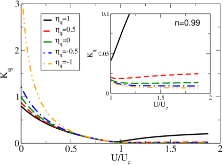
Figure 1: $d=\infty$ - Charge susceptibility as a function of $U/U_{c}$ for $n=0.99$. The inset shows an enlargement of the high $U$ region.

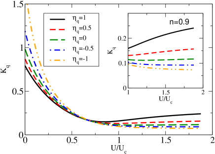
Figure 2: $d=\infty$ - Charge susceptibility as a function of $U/U_{c}$ for $n=0.9$.

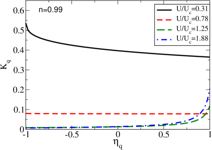
Figure 3: $d=\infty$ - Charge susceptibility as a function of $\eta_{\bf q}$ for $n=0.99$ for various values of the interaction strength $U/U_{c}$.

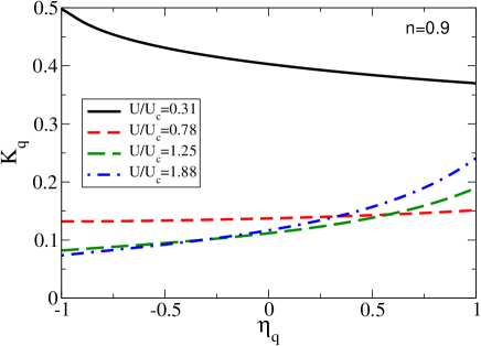
Figure 4: $d=\infty$ - Charge susceptibility as a function of $\eta_{\bf q}$ for $n=0.9$ for various values of the interaction strength $U/U_{c}$.

As discussed in Ref. mul89, , for a generic ${\bf q}$ the corresponding $\eta_{\bf q}$ is trivially zero; only for special ${\bf q}$ $\eta_{\bf q}$ takes values between -1 and +1. In particular for the hypercubic lattice the relevant ${\bf q}$’s are the ones along the diagonal $(0,0,0...)-(\pi,\pi,\pi...)$ (and the other equivalent directions of the hypercubic lattice, which form a set of measure zero). This means that for this infinite dimensional lattice, the study of the momentum depencence of the quantities is sensitive to effects in the (1,1,1…) direction of the Brillouin zone, while it cannot access the other directions like, for instance (1,0,0,0…) or (…0,0,0,1).

In Figs. 1 and 2 we show the dependence on $U$ for selected momenta at $n=0.99$ (almost half-filling) and $n=0.9$ respectively. The curves correspond to different values of the interaction strength in units of the critical $U_{c}=8\sqrt{2/\pi}t$, which is the interaction at which in the infinite dimensional hypercubic lattice electrons undergo the metal-insulator transition at half-filling ($n=1$) in the GA. At small $U$ the susceptibility has a strong enhancement at ${\bf q}_{c}={\bf Q}$, this is due to the nesting of the lattice and leads to the Peierls CDW instability in the presence of coupling to the lattice [Eq. (13)].

Starting from the small-$U$ side, the charge susceptibility is suppressed upon approaching $U_{c}$ and then slightly increases again when $U$ is further increased. The behavior of $\kappa_{\bf q}$ for $U>U_{c}$ strongly depends on momentum and the suppression is most effective for large $q$ and close to half-filling.

Perfect nesting occurs only at half-filling due to the matching of the Fermi (hyper)surface when translated by ${\bf Q}$. In analogy with low dimensional systems one may wonder whether away from half-filing an incommensurate CDW is favored.

Figs. 3 and 4 show the momentum dependence of the susceptibility for density $n=0.99$ and $n=0.9$ and various values of $U/U_{c}$, respectively.

At small $U$ one finds the nesting-induced enhancement at ${\bf q}={\bf Q}$ for both fillings indicating that incommensurate CDW formation is not favored. i.e. there is no shift of ${\bf q}_{c}$.

Interestingly at large $U$ another instability enters into play since in this limit $\kappa_{\bf q}$ acquires a maximum at $\eta_{\bf q}=1$. One qualitatively recovers a momentum structure similar to what is obtained within the large-N expansion of the Hubbard model for $U=\infty$ Koc01 ; Sei00 . In this case the residual repulsion between quasiparticles is most effective at large momenta leading to a suppression of $\kappa_{\bf q}$ for $\eta_{\bf q}\to-1$. Inclusion of a Holstein coupling would induce a PS instability in this limit. The momentum dependence of the susceptibility becomes weak for intermediate values of $U$, slightly below $U_{c}$. All these features are most pronounced upon approaching half-filling.

The fact that for small $U/U_{c}$ the instability momentum is pinned at ${\bf Q}$ is specific to a high-dimensional system, where the effects of nesting of the Fermi surface are weak and the effects of doping in changing the Fermi surface are negligible. We will see in the next section that this is not the case in 2d, where upon doping ${\bf q}_{c}$ moves away from the (1,1) direction and shifts along the (1,0) direction.

From Figs. 3 and 4 we conclude that when $U$ is increased beyond a value of about $0.78U_{c}$ the maximum in the charge response moves from large to small momenta. This signals that the inclusion of (momentum-independent) phonons would drive the system towards a PS instability at large $U$’s, while at small $U$’s the systems would undergo a transition to a CDW state. The behavior of the charge response also allows to infer that the $e$-$e$ correlations suppress more severely the $e$-$ph$ coupling at large momentum transfer than at small transferred momenta. This is the reason why, upon increasing $U$, the system will undergo more easily a low-momentum instability (PS), rather than becoming unstable at finite (and usually large) momenta.

V Results in two dimensions

We now move to the 2d case, which is relevant for many layered materials. We typically worked with a $100\times 100$ lattice for our computations.

We start by characterizing the Peierls instability in 2d. For small $U$ and $n=1$ the charge susceptibility has the Peierls peak at ${\bf q}=(\pi,\pi)$, associated with the Fermi surface nesting. For the doped system the response exhibits a peak for a ${\bf q}_{c}$ close to $(\pi,\pi)$, featuring the tendency to develop an incommensurate CDW in the presence of phonons (Fig. 5, full line). The momentum of the instability undergoes a shift in the $(1,0)$ direction of the Brillouin zone. For small $U$ the peak is located at ${\bf q}_{c}=(\alpha(\delta)\pi,\pi)$ with

$$\alpha(\delta)=1-0.46\delta-1.30\delta^{2}...\sim 1-\delta/2.$$

This depends little on $U$ at weak coupling due to the weak ${\bf q}$-dependency of $W_{\bf q}$ close to $n=1$. A behaviour compatible to ours has been found also for the 2d-Holstein modelVek92 with QMC and RPA calculations on a $8\times 8$ lattice.

Along the (1,0) direction $\kappa_{\bf q}$ exhibits another peak at ${\bf q}^{\prime}_{c}$ (the peak close to ${\bf q}=(0,0)$, full line in Fig. 5). This corresponds to the scattering between states at the (rounded) corners of the Fermi surface in adjacent Brillouin zones. Upon increasing $U$ (cf. Fig. 5), the nesting induced peak structure gets lost. Simultaneously the response at large wave-vectors becomes suppressed and overcome by that at ${\bf q}=(0,0)$. This indicates that the order of the instabilities is reversed like in the $d=\infty$ case: For large $U$ the system phase separates before the CDW instability arises. This behavior will become more clear upon analyzing the charge susceptibility as a function of filling and interaction.

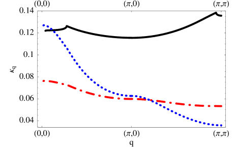
Figure 5: 2d-Charge susceptibility for $n=0.9$ along the open path ${\bf q}=(0,0)-(\pi,0)-(\pi,\pi)$ for $U/U_{c}=0.5$ (solid line), $U/U_{c}=0.9$ (dot-dashed line) and $U/U_{c}=2$ (dotted line).

In Fig. 6 we show the charge compressibility in 2d as a function of $U/U_{c}$ with $U_{c}=128t/\pi^{2}$.

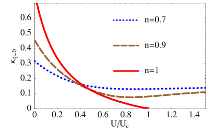
Figure 6: 2d-Charge compressibility as a function of $U/U_{c}$ for various fillings.

For $U=0$ the compressibility is given by the noninteracting density of states at the Fermi energy. The latter diverges for $n\rightarrow 1$ due to the Van Hove singularity. For $U$ close to $U_{c}$ one recovers a similar behavior as in $d=\infty$. The compressibility vanishes at the Mott transition point and has a minimum close to $U_{c}$ for $n\neq 1$.

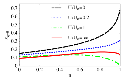
Figure 7: 2d-Charge compressibility as a function of $n$ for various $U/U_{c}$.

In Fig. 7 we present the compressibility as a function of $n$ for different values of $U/U_{c}$. For $n\rightarrow 0$ the compressibility can be computed exactly using a low density expansionfab91 . The ground state energy reads

$$\frac{E}{N}=\pi tn^{2}-2\pi t\frac{n^{2}}{\ln(n)}+...$$

where the second term is the leading correction due to interactions. Computing the compressibility as $\kappa_{{\bf q}=0}^{-1}=\partial^{2}E/\partial n^{2}/N$ one finds that the zero density limit is given by the noninteracting compressibility

$$\kappa_{{\bf q}=0}(n\rightarrow 0)=(2\pi t)^{-1}.$$

In GA+RPA we find instead a small suppression of the zero density compressibility with interaction. This is not surprising since RPA is expected to break down in the low density limit. Still this dependence is quite small and we expect that our results are accurate at moderate densities.

For small $U$ the compressibility is an increasing function of $n$ and reaches the maximum value for $n=1$ as a consequence of the van Hove enhancement. For $U=U_{c}$, $\kappa_{{\bf q}=0}$ goes to zero for $n=1$; for larger $U>U_{c}$, $\kappa_{{\bf q}=0}$ flattens, still exhibiting a smooth maximum for finite doping. Therefore the GA compressibility has a jump discontinuity for $n=1$ and $U>U_{c}$: its left and right limits are finite, while it vanishes at $n=1$. note1

The qualitatively different behaviour of the compressibility for small $U$ and large $U$ is clear: for low fillings the system is weakly affected by $e$-$e$ interactions and its compressibility increases with $n$ no matter how large $U$ is. Approaching half-filling the correlated nature of the system becomes relevant and reduces the compressibility of the electron liquid around $n=1$. One should also keep in mind that close to half-filling AF correlations will become relevant.

In Fig. 8 we show the charge susceptibility $\kappa_{\bf q}$ as a function of $U/U_{c}$ for $n=1$ and $n=0.9$ and selected momenta.

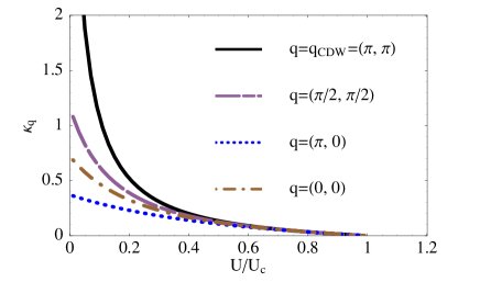
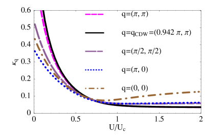
Figure 8: 2d-Charge susceptibility as a function of $U/U_{c}$ for $n=1$ (top) and $n=0.9$ (bottom).

At small momenta the charge susceptibility is close to the compressibility in both cases. As the momentum approaches ${\bf q}={\bf q}_{c}$ the charge susceptibility takes its highest values for small $U$. In particular for $n=1$ (perfect nesting) and $U=0$ the charge susceptibility diverges indicating that an infinitesimal $\lambda$ renders the system unstable. The susceptibility, however, is strongly suppressed by $U$ and at half-filling for any momentum goes to zero for $U=U_{c}$. Therefore, as for $d=\infty$, $e$-$e$ interactions renormalize the noninteracting CDW instability which thus needs a finite $\lambda$ to occur.

At small doping $\kappa_{\bf q}$ is finite and shows a shallow minimum close to $U=U_{c}$. As in $d=\infty$ we see from the larger $\kappa_{\bf q}$ that for $U\gtrsim U_{c}$ the PS instability becomes dominant.

The dominance of the PS instability at large $U$ can be understood from the strong coupling results close to $n=1$. In this case we expect Eq. (47), derived for $n=1$, to be a good approximation. For $U\gg U_{c}$, $\kappa^{0}_{\bf q}A_{\bf q}$ takes large values; then, using Eq. (47), we find simply that the compressibility saturates as a function of $U$ at a value $\kappa_{\bf q}\approx 1/A_{\bf q}$ giving a maximum in $\kappa_{\bf q}$ at ${\bf q}=0$ (cf. Eq. (61)). Our results are consistent with Ref. CDCG95, where C. Castellani et al. find PS in a $U=\infty$ slave boson (SB) investigation at $T=0$. On the other hand, SB calculations for 2-d systems Koc04 ; Cap04 have found PS for $T\approx t$ even in the absence of phonons, while for lower $T$ an homogeneous state is preferred again. This reentrant behavior has not been confirmed by other techniques and should be taken with care due to the poor performance of mean-field SB techniques at finite $T$.

To illustrate the strong coupling behavior, in Fig. 9 we show the charge susceptibility for $U/U_{c}=100$ along the open path ${\bf q}=(0,0)-(\pi,0)-(\pi,\pi)$.

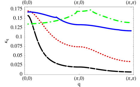
Figure 9: 2d-Charge susceptibility for $U/U_{c}=100$ along the open path ${\bf q}=(0,0)-(\pi,0)-(\pi,\pi)$ for $n=0.98$ (dashed line), $n=0.9$ (dotted line), $n=0.7$ (solid line) and $n=0.4$ (dotted-dashed line).

If we consider fillings quite close to $n=1$, the Coulombic repulsion completely suppresses the CDW peaks which upon doping become visible again for $n\sim 0.7$. Clearly, more evident CDW peaks appear for lower fillings: for $n\ll 1$, the effects of $e$-$e$ interactions are weak even for very large $U$. For $n<0.5$, we find that the ground state is a CDW and that the susceptibility exhibits quite different features with respect to the fillings $n\gtrsim 0.7$.

The most noticeable feature of Fig. 9 is the peak in $\kappa_{\bf q}$ centered at ${\bf q}=(0,0)$: it gets narrower as the doping $\delta$ goes to zero. Therefore upon reducing $\delta$ the charge response to a local perturbation spreads more and more out in space and the small ${\bf q}$ peak width is a measure for the corresponding inverse screening length. We can give an analytical interpretation of this behaviour, using the approximate relation $\kappa_{\bf q}\approx 1/A_{\bf q}$ for $\delta\ll 1$ and adopting for $A_{\bf q}$ its $U=\infty$ form (see Sect. III.2). We have checked that for low doping the $U=\infty$ form of $1/A_{\bf q}$ gives a quite accurate representation for the whole $\kappa_{\bf q}$ curve. In particular, if we consider the low $q$ expansion of $1/A_{\bf q}$, we observe that the ${\bf q}=(0,0)$ peak of the susceptibility is well fitted by a Lorentzian peak of half-width $\tilde{q}=\sqrt{8\delta}$ in the $x$- and $y$-directions. It is worth noting that the typical momentum associated to the peak depends only on the doping $\delta$ and not on the energy $e^{0}$. In the low $q$ limit a relation $\tilde{q}\sim\sqrt{\delta}$ can also be found using the $U=\infty$ single SB quasiparticle interaction.Sei00

All these considerations on the pure electronic response lead us to the phase diagram of the $e$-$ph$ system in Fig. 10.

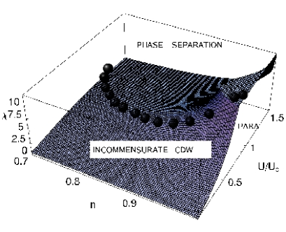
Figure 10: Instability surface $\lambda(n,U/U_{c})$ of the paramagnet towards CDW and PS: the sphered-line marks the transition between the CDW state and the state with PS.

The main outcome is that the large $e$-$e$ interaction changes the nature of the charge instability from an incommensurate CDW to a PS. At large $U\gtrsim U_{c}$ and moderate doping this effect already occurs for small values of the bare $e$-$ph$ coupling $\lambda$. This is the result of a compromise between a reduced quasiparticle kinetic energy (which renders the system prone to instabilities) and the modest screening of the $e$-$ph$ coupling, when one is away from the Mott-insulating phase at half-filling. The fact, that the screening is less important at small transferred momenta obviously favors the occurrence of PS at ${\bf q}_{c}=0$ with respect to the incommensurate CDW.

In case of the 2-d systems we now consider explicitly the renormalized $e$-$ph$ coupling $g_{\bf q}=z_{0}^{2}\Gamma_{\bf q}$ for the bare electrons. In Fig. 11 we show the behaviour of the quantity $g_{\bf q}$ as a function of the $e$-$e$ interaction.

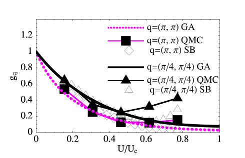
Figure 11: 2d-Renormalized $e$-$ph$ coupling as a function of $U/U_{c}$ for $n\approx 0.88$ at two different momenta. For comparison we report the results obtained at finite T ($T=0.5$) with SB Koc04 (empty symbols) and QMC Hua03 (filled symbols) (these latters are for finite Matsubara electron frequency $\omega=\pi/2$). All the results are obtained for a $8\times 8$ lattice (see Fig. 3 of Ref. Koc04, and Fig. 4a of Ref. Hua03, ).

The trend is quite clear: the suppression of the bare $e$-$ph$ coupling is stronger for large $q$. We compare our results at $T=0$ with SB Koc04 and QMC Hua03 calculations at $T=0.5$ (these latters are also performed at a finite Matsubara frequency of the incoming and outgoing fermions $\omega=\pi T$). The agreement is generically quite good. However, in the finite-T results an upturn of $g_{\bf q}$ is also present (more pronounced for small ${\bf q}$), which was interpreted in Ref. Koc04, as the signature of an incipient PS, which then disappears at zero temperature (besides our findings, for $T=0$ other different treatments find that the ground state is homogeneous Hua03 ; Koc04 ; Cap04 ). The nature of this reentrant behavior is still unclear.

In Fig. 12 we show the vertex $g_{\bf q}$ for different $U$ along a triangular path.

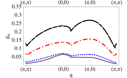
Figure 12: 2d-Renormalized $e$-$ph$ coupling for $n=0.9$ along the closed path ${\bf q}=(\pi,\pi)-(0,0)-(\pi,0)$ for $U/U_{c}=0.46$ (dashed line), $U/U_{c}=0.62$ (dotted-dashed line), $U/U_{c}=0.93$ (dotted line) and $U/U_{c}=1.23$ (solid line). Results are given for a $1000\times 1000$ lattice.

This quantity displays minima at wavevectors ${\bf q}={\bf q}_{c}$ (and at ${\bf q}^{\prime}_{c}$, see Fig.  5) thus suppressing the noninteracting instabilities. These minima arise because the bare susceptibility $\kappa^{0}_{\bf q}$ is maximal at these wavevectors, while the corresponding quantity in the presence of $U$, $\kappa_{\bf q}$ is small due to the suppressed scattering at large momenta when the interaction becomes sizable. On the other hand the charge susceptibility is reduced less at small momenta and this gives rise to the pronounced maximum around ${\bf q}$=(0,0) in the large-$U$ case ($U\gtrsim 0.9$ in Fig. 12). The shape of the curves given in Fig. 12 is very similar to those obtained within a SB calculations at $T=0.002$.Koc04 However, this seeming agreement has to be taken with a pinch of salt since the results shown in Ref. Koc04, are for the quasiparticle-phonon vertex while ours correspond to the vertex for bare electrons and thus should differ by a factor $z_{0}^{2}$.

VI Conclusions

In this work we have investigated the effects of strong electronic correlations on the $e$-$ph$ coupling, in particular we considered the case of phonons coupled to the local charge density as described by the Hubbard-Holstein model. We first exploited the adiabatic limit of the lattice degrees of freedom to derive an exact result relating the screening of the $e$-$ph$ coupling to the purely electronic static charge susceptibility. This result holds generically for any kind of $e$-$e$ interaction (not only for the Hubbard one) and should also provide valuable information in the partially adiabatic case of finite phonon frequency ($\omega_{0}\ll t$). It is important to note that the analysis of the correlation-driven screening of the $e$-$ph$ coupling can be performed by investigating the purely electronic problem. The latter was investigated within the static limit of the GA+RPA method. This technique assumes a Fermi-liquid ground state and considers the low-energy quasiparticle physics. Therefore our low-energy description of the electron liquid is appropriate in high dimensions, where the Fermi-liquid is a good starting point. Particularly favorable is the $d=\infty$ case, where the GA becomes the exact solution of the GZW variational problem.

The main outcome is that (strong) correlations induce rigidity in the charge density fluctuations thereby reducing the effective $e$-$ph$ coupling when this is of the Holstein type. More specifically the analysis of the momentum dependence shows that the $e$-$ph$ coupling is more severely reduced in processes with large momentum transfer. This result, which was already known in large-N approaches to the infinite-$U$ Hubbard-Holstein models, Gri94 ; Kel95 ; Zey96 is considered here within a systematic variation of the correlation strength. In particular, from Figs. 11 and 12 one can see that, while at small $U$’s the effective $e$-$ph$ vertices at small and large transferred momenta differ at most by 40 percent, at large $U$’s the $e$-$ph$ coupling at large momenta can be five or more times smaller than the couplings at low momenta. The fact that the $e$-$ph$ is screened less for small transferred momenta has important consequences as far as the charge instabilities of the model are concerned. Indeed, the $e$-$e$ interaction not only generically reduces the effect of the phonons and enhances the minimum strength of $e$-$ph$ coupling to drive the system unstable, but also introduces a momentum dependence, which changes the nature of the instability upon increasing the strength of the correlation: While for small $e$-$e$ interaction the leading instability is of the Peierls type, with the formation of CDW at momenta $|{\bf q}_{c}|=2k_{F}$, upon increasing $U$, the scattering processes at small transferred momentum become comparatively stronger and lead to a PS instability at vanishing ${\bf q}_{c}$. Our technique allows a systematic investigation of how the low-coupling CDW instability transforms into the PS instability leading to a phase diagram like tha one shown in Fig. 10 for the 2-d system.

Of course the PS instability is specific to the short range nature of the model. When the long range Coulomb interaction is included the large-scale PS of charged holes is prevented and a frustrated PS occurs with the formation of various possible textures CDCG95 ; Sei00 ; lor01I ; lor02 ; Ort06 ; Ort07 ; ort08 .

We also notice that the bare $e$-$ph$ $\lambda$ needed to drive the systems unstable are rather small (of order one or less) at large $U$ and moderate doping. A good compromise is indeed reached in this region, where the quasiparticles have a substantially reduced kinetic energy (the effective mass is 3-5 times larger than the bare one), but the system is not too close to the insulating phase, where the interaction would screen too severely the $e$-$ph$ coupling. Therefore, in this rather metallic regime the (frustrated) PS instability is quite competitive with respect to the polaron formation, which could instead be favored by the stronger correlation effects occurring in the antiferromagnetic region of the phase diagramMCgunnarson .

The general interest of the above findings and the encouraging reliability test of the GA technique discussed in the present work are a stimulating support for the extension of the present work to the dynamical regime. In this case future natural extensions will consider the analysis of correlation effects on the phonon dynamics and their investigation in broken-symmetry states, like the stripe phase.

APPENDIX

Real space energy expansion

Here we give a derivation of the second order term $\delta E_{e}^{(2)}$ in the energy expansion Eq. (31). In real space we obtain

$$\delta E_{e}^{(2)}=\sum_{ij}t_{ij} \{ \frac{1}{2}z_{0}[z^{{}^{\prime}}(\delta\rho_{ii}\delta T_{ij}^{C}+\delta m_{i}\delta T_{ij}^{S})+z^{{}^{\prime}}_{+-}(\delta\rho_{ii}\delta T_{ij}^{C}-\delta m_{i}\delta T_{ij}^{S})]$$ (66)

$$+ \frac{1}{8}T_{ij0}[(z^{{}^{\prime}}+z^{{}^{\prime}}_{+-})^{2}\delta\rho_{ii}\delta\rho_{jj}+(z^{{}^{\prime}}-z^{{}^{\prime}}_{+-})^{2}\delta m_{i}\delta m_{j}+z_{0}(z^{{}^{\prime\prime}}_{++}+2z^{{}^{\prime\prime}}_{+-}+z^{{}^{\prime\prime}}_{--})(\delta\rho_{ii})^{2}$$

$$+ z_{0}(z^{{}^{\prime\prime}}_{++}-2z^{{}^{\prime\prime}}_{+-}+z^{{}^{\prime\prime}}_{--})(\delta m_{i})^{2}]+\frac{1}{2}T_{ij0}[z^{{}^{\prime}}_{D}(z^{{}^{\prime}}+z^{{}^{\prime}}_{+-})\delta\rho_{ii}\delta D_{j}+z_{0}(z^{{}^{\prime\prime}}_{+D}+z^{{}^{\prime\prime}}_{-D})\delta\rho_{ii}\delta D_{i}]$$

$$+ z_{0}z^{{}^{\prime}}_{D}\delta T_{ij}^{C}\delta D_{i}+\frac{1}{2}T_{ij0}[(z^{{}^{\prime}}_{D})^{2}\delta D_{i}\delta D_{j}+z_{0}z^{{}^{\prime\prime}}_{D}(\delta D_{i})^{2}]\ \ \}$$

where the fluctuating variables correspond to the charge density $\rho_{ii}=\rho_{ii\uparrow}+\rho_{ii\downarrow}$ and the magnetization density $m_{i}=\rho_{ii\uparrow}-\rho_{ii\downarrow}$. Further on we have defined the transitive fluctuations

$$T_{ij}=T_{ij0}+\delta T_{ij}^{C}+\delta T_{ij}^{S}$$

which in the charge- and spin sector read as

$$\delta T_{ij}^{C}=\sum_{\sigma}(\delta\langle c^{{\dagger}}_{i\sigma}c_{j\sigma}\rangle+\delta\langle c^{{\dagger}}_{j\sigma}c_{i\sigma}\rangle)$$

$$\delta T_{ij}^{S}=\sum_{\sigma}\sigma(\delta\langle c^{{\dagger}}_{i\sigma}c_{j\sigma}\rangle+\delta\langle c^{{\dagger}}_{j\sigma}c_{i\sigma}\rangle).$$

Since we study a paramagnetic system it is convenient to define the following abbreviations for the z-factors and its derivatives:

$$z_{i\sigma}\equiv z_{0},\ \ \frac{\partial z_{i\sigma}}{\partial\rho_{ii\sigma}}\equiv z^{{}^{\prime}},$$

$$\frac{\partial z_{i\sigma}}{\partial\rho_{ii-\sigma}}\equiv z^{{}^{\prime}}_{+-},\ \frac{\partial z_{i\sigma}}{\partial D_{i}}\equiv z^{{}^{\prime}}_{D}$$

$$\frac{\partial^{2}z_{i\sigma}}{\partial\rho^{2}_{ii\sigma}}\equiv z^{{}^{\prime\prime}}_{++},\ \frac{\partial^{2}z_{i\sigma}}{\partial\rho_{ii\sigma}\partial\rho_{ii-\sigma}}\equiv z^{{}^{\prime\prime}}_{+-},\ \frac{\partial^{2}z_{i\sigma}}{\partial\rho^{2}_{ii-\sigma}}\equiv z^{{}^{\prime\prime}}_{--}$$

$$\frac{\partial^{2}z_{i\sigma}}{\partial D^{2}_{i}}\equiv z^{{}^{\prime\prime}}_{D},\ \frac{\partial^{2}z_{i\sigma}}{\partial\rho_{ii\sigma}\partial D_{i}}\equiv z^{{}^{\prime\prime}}_{+D},\ \frac{\partial^{2}z_{i\sigma}}{\partial\rho_{ii-\sigma}\partial D_{i}}\equiv z^{{}^{\prime\prime}}_{-D}$$

For the half-filled paramagnetic state we have $z^{{}^{\prime}}=z^{{}^{\prime}}_{+-}$ and $z^{{}^{\prime\prime}}_{+D}=z^{{}^{\prime\prime}}_{-D}$.

Momentum space energy expansion

We transform Eq. (66) into momentum space. For the paramagnetic system the expansion separates into the charge- and spin sector $\delta E_{e}^{(2)}=\delta E_{e}^{S}+\delta E_{e}^{C}$.

In the spin sector we find:

$$\delta E_{e}^{S}=\frac{1}{N}\sum_{{\bf q}} [ \frac{1}{2}z_{0}(z^{{}^{\prime}}-z^{{}^{\prime}}_{+-})(\delta S^{z}_{\bf q}\delta T^{S}_{-{\bf q}}+$$ (67)

$$+ \delta T^{S}_{\bf q}\delta S^{z}_{-{\bf q}})+N_{\bf q}\delta S^{z}_{\bf q}\delta S^{z}_{-{\bf q}}\ \ ]$$

with the following definitions:

$$\delta m_{i}=\frac{1}{N}\sum_{{\bf q}}e^{i{\bf q}_{i}\cdot{\bf r}_{i}}\delta m_{{\bf q}}=\frac{2}{N}\sum_{{\bf q}}e^{i{\bf q}_{i}\cdot{\bf r}_{i}}\delta S^{z}_{{\bf q}}$$

$$N_{\bf q}=\frac{1}{N} [ (z^{{}^{\prime}}-z^{{}^{\prime}}_{+-})^{2}\sum_{{\bf k}\sigma}\epsilon^{0}_{{\bf k}+{\bf q},\sigma}n_{{\bf k}\sigma}$$

$$+ z_{0}(z^{{}^{\prime\prime}}_{++}-2z^{{}^{\prime\prime}}_{+-}+z^{{}^{\prime\prime}}_{--})\sum_{{\bf k}\sigma}\epsilon^{0}_{{\bf k}\sigma}n_{{\bf k}\sigma}\ \ ]$$

The form of $\delta E_{e}^{C}$ in momentum space is slightly more complicate:

$$\delta E_{e}^{C} = \frac{1}{2N}z_{0}(z^{{}^{\prime}}+z^{{}^{\prime}}_{+-})\sum_{{\bf q}}\delta\rho_{{\bf q}}\delta T^{C}_{-{\bf q}}$$ (68)

$$+ \frac{1}{4N^{2}}\sum_{{\bf k}{\bf q}\sigma}[(z^{{}^{\prime}}+z^{{}^{\prime}}_{+-})^{2}\epsilon^{0}_{{\bf k}+{\bf q},\sigma}n_{{\bf k}\sigma}+(z^{{}^{\prime\prime}}_{++}+2z^{{}^{\prime\prime}}_{+-}+z^{{}^{\prime\prime}}_{--})z_{0}\epsilon^{0}_{{\bf k}\sigma}n_{{\bf k}\sigma}]\delta\rho_{{\bf q}}\delta\rho_{-{\bf q}}$$

$$+ \frac{1}{N^{2}}\sum_{{\bf k}{\bf q}\sigma}[z^{{}^{\prime}}_{D}(z^{{}^{\prime}}+z^{{}^{\prime}}_{+-})\epsilon^{0}_{{\bf k}+{\bf q},\sigma}n_{{\bf k}\sigma}+z_{0}(z^{{}^{\prime\prime}}_{+D}+z^{{}^{\prime\prime}}_{-D})]\delta\rho_{{\bf q}}\delta D_{-{\bf q}}$$

$$+ \frac{1}{N}\sum_{{\bf q}}z_{0}z^{{}^{\prime}}_{D}\delta D_{{\bf q}}\delta T^{C}_{-{\bf q}}+\frac{1}{N^{2}}\sum_{{\bf k}{\bf q}\sigma}[(z^{{}^{\prime}}_{D})^{2}\epsilon^{0}_{{\bf k}+{\bf q},\sigma}n_{{\bf k}\sigma}+z_{0}z^{{}^{\prime\prime}}_{D}\epsilon^{0}_{{\bf k}\sigma}n_{{\bf k}\sigma}]\delta D_{{\bf q}}\delta D_{-{\bf q}}$$

From Eq. (68), we recover Eq. (53) by using the definitions of $L_{\bf q}$, $U_{\bf q}$ and $V_{\bf q}$ from Eq. 54.

References

- (1) A. Lanzara, P. V. Bogdanov, X. J. Zhou, S. A. Kellar, D. L. Feng, E. D. Lu, T. Yoshida, H. Eisaki, A. Fujimori, K. Kishio, J.-I. Shimoyama, T. Noda, S. Uchida, Z. Hussain, and Z. X. Shen, Nature (London) 412, 510 (2001).
- (2) M. D’Astuto, P. K. Mang, P. Giura, A. Shukla, P. Ghigna, A. Mirone, M. Braden, M. Greven, M. Krisch, , and F. Sette, Phys. Rev. Lett. 88, 167002 (2002).
- (3) G.-H. Gweon, T. Sasagawa, S. Y. Zhou, J. Graf, H. Takagi, D.-H. Lee, and A. Lanzara, Nature (London) 430, 187 (2004).
- (4) D. Reznik, L. Pintschovius, M. Ito, S. Iikubo, M. Sato, H. Goka, M. Fujita, K. Yamada, G. D. Gu, and J. M. Tranquada, Nature (London) 440, 1170 (2006).
- (5) D. Reznik, T. Fukuda, D. Lamago, A. Q. R. Baron, S. Tsutsui, M. Fujita, and K. Yamada, arxiv:cond-mat/0710.4782 (unpublished).
- (6) J. Lee, K. Fujita, K. McElroy, J. A. Slezak, M. Wang, Y. Aiura, H. Bando, M. Ishikado, T. Masui, J.-X. Zhu, A. V. Balatsky, H. Eisaki, S. Uchida, and J. C. Davis, Nature (London) 442, 546 (2006).
- (7) J. P. Falck, A. Levy, M. A. Kastner, and R. J. Birgeneau, Phys. Rev. Lett. 69, 1109 (1992).
- (8) P. Calvani, M. Capizzi, S. Lupi, P. Maselli, A. Paolone, and P. Roy, Phys. Rev. B 53, 2756 (1996).
- (9) P. Calvani, M. Capizzi, S. Lupi, and G. Balestrino, Europhys. Lett. 31, 473 (1995).
- (10) A. J. Millis, R. Mueller, and B. I. Shraiman, Phys. Rev. B 54, 5405 (1996).
- (11) P. S. Cornaglia, H. Ness, and D. R. Grempel, Phys. Rev. Lett. 93, 147201 (2004).
- (12) O. Gunnarsson, Rev. Mod. Phys. 69, 575 (1997).
- (13) M. Capone, M. Fabrizio, C. Castellani, and E. Tosatti, Science 296, 2364 (2002).
- (14) M. Grilli and C. Castellani, Phys. Rev. B 50, 16880 (1994).
- (15) C. Castellani, C. D. Castro, and M. Grilli, Phys. Rev. Lett. 75, 4650 (1995).
- (16) J. Lorenzana, C. Castellani, and C. Di Castro, Phys. Rev. B 64, 235127 (2001).
- (17) J. Lorenzana, C. Castellani, and C. Di Castro, Europhys. Lett. 57, 704 (2002).
- (18) U. Löw, V. J. Emery, K. Fabricius, and S. A. Kivelson, Phys. Rev. Lett. 72, 1918 (1994).
- (19) J. Lorenzana, C. Castellani, and C. Di Castro, Phys. Rev. B 64, 235128 (2001).
- (20) C. Ortix, J. Lorenzana, and C. Di Castro, Phys. Rev. B 73, 245117 (2006).
- (21) C. Ortix, J. Lorenzana, M. Beccaria, and C. Di Castro, Phys. Rev. B 75, 195107 (2007).
- (22) C. Ortix, J. Lorenzana, and C. Di Castro, Phys. Rev. Lett. xx, xxx (2008), ”in press”.
- (23) J. E. Hirsch and D. J. Scalapino, Phys. Rev. Lett. .
- (24) J. E. Hirsch and D. J. Scalapino, Phys. Rev. B 29, 5554 (1984).
- (25) J. E. Hirsch, Phys. Rev. B 31, 6022 (1985).
- (26) E. Berger, P. Valáek, and W. von der Linden, Phys. Rev. B 52, 4806 (1995).
- (27) Z. B. Huang, W. Hanke, and E. Arrigoni, Phys. Rev. B 68, 220507 (2003).
- (28) J. E. Hirsch, Phys. Rev. Lett. 51, 296 (1983).
- (29) A. Dobry, A. Greco, J. Lorenzana, and J. Riera, Phys. Rev. B 49, 505 (1994).
- (30) A. Dobry, A. Greco, J. Lorenzana, J. Riera, and H. T. Diep, EPL (Europhysics Letters) 27, 617 (1994).
- (31) M. Capone, M. Grilli, and W. Stephan, Eur. Phys. J. B 11, 551 (1999).
- (32) J. Lorenzana and A. Dobry, Phys. Rev. B 50, 16094 (1994).
- (33) J. K. Freericks and M. Jarrell, Phys. Rev. Lett. 75, 2570 (1995).
- (34) M. Capone, G. Sangiovanni, C. Castellani, C. D. Castro, and M. Grilli, Phys. Rev. Lett. 92, 106401 (2004).
- (35) W. Koller, D. Meyer, Y. no, and A. C. Hewson, Europhys. Lett. 66, 559 (2004).
- (36) W. Koller, D. Meyer, and A. C. Hewson, Phys. Rev. B 70, 155103 (2004).
- (37) G. S. Jeon, T.-H. Park, J. H. Han, H. C. Lee, and H.-Y. Choi, Phys. Rev. B 70, 125114 (2004).
- (38) G. Sangiovanni, M. Capone, C. Castellani, and M. Grilli, Phys. Rev. Lett. 94, 026401 (2005).
- (39) G. Sangiovanni, M. Capone, and C. Castellani, Phys. Rev. B 73, 165123 (2006).
- (40) J. Keller, C. E. Leal, and F. Forsthofer, Physica B 206 & 207, 739 (1995).
- (41) R. Zeyher and M. L. Kuli, 53 2850, 53 (1996).
- (42) This characteristic behavior of the GA charge compressibility holds in every dimension.
- (43) E. Koch and R. Zeyher, Phys. Rev. B 70, 094510 (2004).
- (44) E. Cappelluti, B. Cerruti, and L. Pietronero, Phys. Rev. B 69, 161101 (2004).
- (45) R. Citro and M. Marinaro, Eur. Phys. J. B 20, 343 (2001).
- (46) R. Citro, S. Cojocaru, and M. Marinaro, Phys. Rev. B 72, 115108 (2005).
- (47) M. C. Gutzwiller, Phys. Rev. Lett. 10, 159 (1963).
- (48) F. Günther, G. Seibold, and J. Lorenzana, Phys. Rev. Lett. 98, 176404 (2007).
- (49) W. Metzner and D. Vollhardt, Phys. Rev. B 37, 7382 (1988).
- (50) F. Gebhard, Phys. Rev. B 41, 9452 (1990).
- (51) G. Seibold and J. Lorenzana, Phys. Rev. Lett. 86, 2605 (2001).
- (52) D. Vollhardt, Rev. Mod. Phys. 56, 99 (1984).
- (53) G. Seibold, F. Becca, and J. Lorenzana, Phys. Rev. B 67, 085108 (2003).
- (54) G. Seibold, F. Becca, P. Rubin, and J. Lorenzana, Phys. Rev. B 69, 155113 (2004).
- (55) G. Seibold, F. Becca, and J. Lorenzana, Phys. Rev. Lett. 100, 016405 (2008).
- (56) J. Lorenzana and G. Seibold, Phys. Rev. Lett. 89, 136401 (2002).
- (57) J. Lorenzana and G. Seibold, Phys. Rev. Lett. 90, 066404 (2003).
- (58) G. Seibold and J. Lorenzana, Phys. Rev. Lett. 94, 107006 (2005).
- (59) G. Kotliar and A. E. Ruckenstein, Phys. Rev. Lett. 57, 1362 (1986).
- (60) J. P. Blaizot and G. Ripka, Quantum Theory of Finite Systems (The MIT Press, Cambridge, Massachusetts, 1986).
- (61) P. Ring and P. Schuck, The nuclear many-body problem (Springer-Verlag, New York, 1980).
- (62) P. Noziéres and D. Pines, The Theory of Quantum Liquids (Addison-Wesley Publishing Company, Inc, ADDRESS, 1990).
- (63) W. F. Brinkman and T. M. Rice, Phys. Rev. B 2, 4302 (1970).
- (64) E. Müller-Hartmann, Z. Phys. B 74, 507 (1989).
- (65) Handbook of Mathematical Functions, edited by M. Abramowitz and I. A. Stegun (Dover Publications, New York, 1965).
- (66) G. Seibold, F. Becca, F. Bucci, C. Castellani, C. D. Castro, and M. Grilli, Eur. Phys. J. B 13, 87 (2000).
- (67) E. Koch, Phys. Rev. B 64, 165113 (2001).
- (68) M. Vekic̀, R. M. Noack, and S. R. White, Phys. Rev. B 46, 271 (1992).
- (69) M. Fabrizio, A. Parola, and E. Tosatti, Phys. Rev. B 44, 1033 (1991).
- (70) G. Sangiovanni, O. Gunnarsson, E. Koch, C. Castellani, and M. Capone, Phys. Rev. Lett. 97, 046404 (2006).