Significance tests for comparing digital gene expression profiles

Abstract

1 Motivation:

Most of the statistical tests currently used to detect differentially expressed genes are based on asymptotic results, and perform poorly for low expression tags. Another problem is the common use of a single canonical cutoff for the significance level (p-value) of all the tags, without taking into consideration the type II error and the highly variable character of the sample size of the tags.

2 Results:

This work reports the development of two significance tests for the comparison of digital expression profiles, based on frequentist and Bayesian points of view, respectively. Both tests are exact, and do not use any asymptotic considerations, thus producing more correct results for low frequency tags than the $\chi^{2}$ test. The frequentist test uses a tag-customized critical level which minimizes a linear combination of type I and type II errors. A comparison of the Bayesian and the frequentist tests revealed that they are linked by a Beta distribution function. These tests can be used alone or in conjunction, and represent an improvement over the currently available methods for comparing digital profiles.

3 Availability:

Implementations of both tests are available under the GNU General Public License at http://code.google.com/p/kempbasu

4 Contact:

varuzza@gmail.com (L. Varuzza) and cpereira@ime.usp.br (C.A.B. Pereira)

¹Institute of Mathematics and Statistics, Rua do Matão 1010, Bloco A and ²Institute of Biomedical Sciences, University of São Paulo, 05508-090, São Paulo SP, Brazil

5 Introduction

Crucial events in the biology of living organisms, such as cell differentiation and specialization, depend on minute variations of gene expression under different conditions and/or temporal events. A key approach to elucidate a gene function is to quantify and compare the expression level of a large set of genes in different tissues or developmental stages, or under different conditions/treatments. This task can be performed using large-scale hybridization to microarrays, or by counting gene tags or signatures using methods such as Serial Analysis of Gene Expression (SAGE), developed by Velculescu et al. (1995), and Massively Parallel Signature Sequencing (MPSS), described by Brenner et al. (2000). By comparing transcript expression profiles among different samples, one can identify differentially expressed genes associated with a particular tissue and/or condition. Unlike microarrays analysis, SAGE and MPSS do not require any prior knowledge of the transcript sequences. These techniques provide a digital profiling, and permit to estimate the relative abundance of mRNA molecules of a transcriptome based upon two main premises. First, these methods assume that each position-specific short sequence tag can unequivocally identify its corresponding transcript. Second, that the tag counts are representative of the abundances of the corresponding mRNAs of the transcriptome, that is, every mRNA copy has the same chance of being counted as the corresponding tag of the library. The selection of a specific tag sequence from the total pool of transcripts can be well approximated as a sampling with replacement (Stollberg et al., 2000).

Several statistical tests have been devised to deal with the problem of comparing digital expression profiles and identifying differentially expressed genes (Audic and Claverie, 1997; Baggerly et al., 2004; Robinson and Smyth, 2007; Stekel et al., 2000; Thygesen and Zwinderman, 2006; Vêncio et al., 2004), and reviewed by Man et al. (2000), Romualdi et al. (2001) and Ruijter et al. (2002). Most of these tests, including the $\chi^{2}$ test as the most classical representative, rely on asymptotic methods and, as such, perform poorly when the sample size is small, as is the case of low expression tags. Another problematic aspect of detecting differentially expressed genes by significance tests, is the use of a single critical level, such as the canonical values 0.1, 0.05 and 0.01, which, apart from the common use, do no present any particular advantage. In this work we report the development of two distinct exact significance tests for comparative studies of digital expression profiles. The methods are based on the frequentist and Bayesian points of view, respectively, and are fully implemented on open source programs. Since these significance tests do not use any asymptotic considerations, they produce more correct results for low frequency tags than asymptotic methods. Also, the frequentist test uses a tag-customized critical level which minimizes a linear combination of type I and type II errors. We provide evidences that both methods present very similar results and represent an improvement over the currently available statistical tests.

6 Methods

6.1 Frequentist Significance Test: p-value

As a first approach to address the problem of detecting differentially expressed tags, we propose an exact and novel frequentist significance test. Assuming $k$ ($>1$) libraries, let $M$ be the number of distinct tags and $N_{j}$ the total number of tags in library $j$ ($j=1,2,\cdots,k$). The frequency of the $i$-th tag in the $j$-th library is denoted by $X_{ij}$. Hence, $N_{j}=X_{1j}+X_{2j}+...+X_{Mj}$. The basic statistical model can be stated as:

• For each $j$, the random vector $\mathbf{X}_{\bullet j}=(X_{1j};X_{2j};\cdots;X_{Mj})$ is distributed as a multinomial with parameters $N_{j}$ and $\mathbf{P}_{j}=(p_{1j};p_{2j};\cdots;p_{Mj})$.

• The random vectors $\mathbf{X}_{\bullet 1},\mathbf{X}_{\bullet 2},\cdots,\mathbf{X}_{\bullet k}$ are mutually statistically independent, that is, we assume that the libraries have been collected independently.

• Considering that, for digital expression profiles, parameters $\mathbf{P}_{j}$ and $N_{J}$ usually assume low and high values, respectively, several authors (Audic and Claverie, 1997; Cai et al., 2004; Zhu et al., 2008) have considered that the distribution of tag frequency $X_{ij}$ can be approximated to a Poisson with mean $N_{j}p_{ij}$.

• Assuming that the libraries have been collected independently, the full model for a single tag $i$ is

  $$\text{Pr}\left\{X_{i1}=x_{i1},\cdots,X_{ik}=x_{ik}|p_{i1},\cdots,p_{ik}\right\}=\\ \frac{(N_{1}p_{i1})^{x_{i1}}\cdots(N_{k}p_{ik})^{x_{ik}}}{x_{i1}!\cdots x_{ik}!}\exp(N_{1}p_{i1}+\cdots+N_{k}p_{ik}).$$ (1)

6.1.1 Partial Likelihood

One can now write the equation (1) using an alternative parametrization. Let the new parameters be $\theta_{i}=N_{1}p_{i1}+\cdots+N_{k}p_{ik}$ and $\Pi_{i}=(\pi_{i1};\cdots;\pi_{ik})$, with $\pi_{ij}=N_{j}p_{ij}/\theta_{i}$. Assuming the random variable $Y_{i}=X_{i1}+\cdots+X_{ik}$ and the observation $y_{i}=x_{i1}+\cdots+x_{ik}$, the two following events are equivalent:

$$\left\{X_{i1}=x_{i1},\cdots,X_{ik}=x_{ik}\right\}$$

$$\equiv$$

$$\left\{X_{i1}=x_{i1},\cdots,X_{ik}=x_{ik};Y_{i}=y_{i}\right\}.$$

Therefore, the alternative statistical model can be written as:

$$\text{Pr}\left\{X_{i1}=x_{i1},\cdots,X_{ik}=x_{ik},Y_{i}=y_{i}|\Pi_{i},\theta_{i}\right\}=\\ \frac{y!}{x_{i1}!\cdots x_{ik}!}(\pi_{i1})^{x_{i1}}\cdots(\pi_{ik})^{x_{ik}}\frac{\theta_{i}^{y}e^{-y}}{y!}.$$ (2)

With this new parametrization, the full likelihood becomes the product of a multinomial probability function by a Poisson probability function. It is noteworthy that the new parameters, $\Pi_{i}$ and $\theta_{i}$, are variation independent, i.e., their values carry no information about each other. According to Basu (1977) and Cox (1975), to perform inference about $\Pi_{i}$ (or $\theta_{i}$) one only has to consider as the likelihood the multinomial (or Poisson) factor of equation (2).

Under the full likelihood model, the null hypothesis – tag $i$ has the same expression in all libraries – is

$$H_{0}:P_{i}=(p_{i1},\cdots,p_{ik})=(p_{i},\cdots,p_{i}).$$ (3)

With the new parametrization, the null hypothesis is reduced to a simple hypothesis as follows:

$$H_{0}^{\prime}:\Pi_{i}=\Pi_{0}=\left(\frac{N_{1}}{N},\cdots,\frac{N_{k}}{N}\right).$$ (4)

This approach of partial likelihood, introduced by Cox (1975), simplifies considerably the problem of comparing the expression of the $j$-th tag in all $k$ libraries. Hence, under the null hypothesis, the likelihood is simply a multinomial probability function evaluated for $\Pi_{0}$. Being $X_{i\bullet}=(X_{i1},\cdots,X_{ik})$, the distribution under the null and alternative hypotheses are, respectively,

$$H_{0}^{\prime}:\text{Pr}\{X_{i\bullet}|Y_{i}=y_{i};\Pi_{i}=\Pi_{0}\}=\frac{y_{i}!}{N^{y_{i}}}\prod_{j=1}^{k}\frac{N_{j}^{x_{j}}}{x_{j}!}$$ (5)

and

$$H_{1}^{\prime}:\text{Pr}\{X_{i\bullet}|Y_{i}=y_{i};\Pi_{i}\}=y_{i}!\prod_{j=1}^{k}\frac{\pi_{ij}^{x_{j}}}{x_{j}!}.$$ (6)

6.1.2 Significance Level

According to Cox (1977) and Kempthorne (1976), a significance test is a method that measures the consistency of the data with the null hypothesis. The commonly used index to perform this task is the well known p-value. We refer to Kempthorne and Folks (1971) for important discussions on the evaluation of p-values. For a random vector $\mathbf{X}$, let $T(\mathbf{X})=T$ be a statistic in which small values of T cast doubt about $H_{0}$. For an observation $\mathbf{x}$ with $T(\mathbf{x})=t$, the associated p-value is the probability under $H_{0}$ of the event $\{T\leq t\}$, that is, $p=\text{Pr}\{T\leq t|H_{0}\}$. The consequence of this definition is that the random variable $T$ must be a function that produces an order in the sample space. In this ordered sample space, the sample points with low order favor the alternative hypothesis, whereas those with a higher order support the null hypothesis.

As we will show below, the likelihood ratio is an appropriate statistic for ordering the sample space relative to the null hypothesis. Let $R(\mathbf{X})$ be the maximum of the likelihood function under $H_{0}$ divided by the overall maximum of the likelihood function (eq. 7), and $R(\mathbf{x})=r$ be the value of that statistic at the observation $\mathbf{x}$, the p-value is $\text{Pr}\{R\leq r|H_{0}\}$.

$$R_{i}(\mathbf{X})=\left(\frac{y_{i}}{N}\right)^{y_{i}}\prod_{j=1}^{k}\left(\frac{N_{j}}{x_{j}}\right)^{x_{j}}$$ (7)

As one can conclude, $R$ has the desired property of ordering the sample space according to the support of $H_{0}$. The use of likelihood ratios for computing p-values has been already addressed by Neyman and Pearson (1928), Pereira and Wechsler (1993), and Dempster (1997).

Let’s define the tail set, $T_{i}$, of frequencies more extreme than $\mathbf{x}_{i}$:

$$T_{i}=\left\{\mathbf{w}=(w_{1},\cdots,w_{k})|w_{1}+\cdots+w_{k}=y_{i}\vee R(\mathbf{w})\leq R(\mathbf{x}_{i})\right\}.$$

The p-value of the tag $i$, $pv_{i}$, that provides the significance level for $H_{0}’$ when the observation is $\mathbf{x}_{i}$, is:

$$pv_{i}=\sum_{w\in T_{i}}\frac{y_{i}!}{N^{y_{i}}}\prod_{j=1}^{k}\frac{N_{j}^{w_{j}}}{w_{j}!}.$$ (8)

A serious limitation of this exact p-value calculation is that the number of points in the sample space grows exponentially in regard to the number of dimensions. To overcome this problem, we use an algorithm based on the Monte Carlo method:

p-valueX,N,runs t R̄(X,N)
y ∑̄X_i
p \̄mathbf{missing}N/∑N_i
c 0̄
i 1̄ runs W \̄text{missing}Random vector with Multi(y,p)
R(W,N) ≤t c c̄+1
c/runs

In order to test and validate this method, we developed Kemp, a C language program named after Prof. Oscar Kempthorne, an English statistician who has produced an extensive work on the topic of significance tests.

6.1.3 Critical significance level

In order to have inferential meaning, the evaluation of a significance index should help one to decide in favor or against a null hypothesis. Hence, a decision rule must be stated. For instance, the critical level is the cutoff between reject/accept actions. In any digital expression profile, the relative abundance can vary dramatically from tag to tag, implying that the use of a single critical significance level for all tags may be unfair for those tags with low frequencies. For this reason, we decided to calculate a critical level for each particular tag, according to the recommendations of DeGroot (1986). Thus, we used the optimum procedure of the decision theory, which minimizes the risk function $a\alpha+b\beta$, a linear combination of the two kinds of errors: $\alpha$ and $\beta$, corresponding to errors of type I (false positive) and type II (false negative), respectively.

The value of $\alpha$ is the probability of the critical region using the parameter value defined by the null hypothesis. Conversely, computation of $\beta$ is more complex, since $H_{1}$ is a composed hypothesis rather than a single point hypothesis. To solve the problem of defining the appropriate $\beta$, we considered the average of all possible single hypotheses within the set of alternative hypotheses. To perform this computation, we used a uniform prior for the parameter of the alternative hypothesis, and considered the predictive distribution for this prior choice. Fortunately, the predictive is a uniform discrete distribution in the sample space and, hence, is a constant equal to the inverse of the number of points of the sample space. Therefore, the aforementioned average of $\beta$ is the number of points within the acceptance region, divided by this constant.

To choose the critical level, we considered, for a given value of y, all possible critical regions. The critical level is then the value of $\alpha$ for the critical region that gives the smallest value of each combination $a\alpha+b\beta$. We also defined an arbitrary score S (eq. 9), based on practical results, to order the differentially expressed tags according to the relative “distance” between their corresponding p-value and critical level.

$$S=10\left(1-\frac{pv}{\alpha}\right)$$ (9)

6.2 Bayesian Significance Test: e-value

The FBST, Full Bayesian Significance Test, was introduced by Pereira and Stern (1999). The objective of this method is to obtain an alternative index to p-values, namely e-values (where e stands for evidence). Both indices vary from zero to one, since they represent probabilities on the sample space (p-value) and on the parameter space (e-value). The Bayesian test is defined on the original parameters $\mathbf{P}_{1},\cdots,\mathbf{P}_{k}$ of the libraries. As a prior for these parameters, we considered independent and identical Dirichlet distributions with metaparameters $A_{1},\cdots,A_{M}$. Consequently, the posterior distribution for each independent parameter $\mathbf{P}_{j}$ is Dirichlet with metaparameters $x_{1j}+A_{1},\cdots,x_{Mj}+A_{M}$ (Aitchison, 2003). For this model, the posterior marginal density of the parameter $p_{ij}$ is $Beta(x_{ij}+A_{i},N_{j}+S-x_{ij}-A_{i})$, with $S=A_{1}+\cdots+A_{n}$. From the independency of $P_{j}$, the joint probability of all libraries, for each single tag, is a product of these Beta densities.

To perform this test, one needs two numerical procedures: optimization and integration. The low values of $x_{ij}+A_{i}$, compared to the high values of $N_{j}+S-x_{ij}-A_{i}$, usually lead to an underflow in the numerical integration. Thus, we transformed the Beta densities into logistic-normal distributions (Aitchison, 2003). The mean and the variance of the normal distributions, obtained after the logistic transformation, $\zeta_{ij}=\log[p_{ij}/(1-p_{ij})]$, are presented in eq. 10 and eq. 11, respectively, where $\Psi$ is the digamma and and $\Psi^{\prime}$ is the trigamma functions.

$$\mu_{ij}=\Psi(x_{ij}+A_{i})+\Psi(N_{j}-S-x_{ij}-A_{i})$$ (10)

$$\sigma_{ij}^{2}=\Psi^{\prime}(x_{ij}+A_{i})-\Psi^{\prime}(N_{j}-S-x_{ij}-A_{i})$$ (11)

Notice that the null hypothesis $\zeta_{i1}=\cdots=\zeta_{ik}$ is equivalent to the original hypothesis $p_{i1}=\cdots=p_{ij}$. By using this approach, the integration of the product of Beta distributions is replaced by a integration of normal distributions, whose parameter values avoid numerical representation problems that could arise when using Beta distributions.

The Bayesian significance test was implemented on Basu, a C language program named after Prof. Debabrata Basu, an Indian statistician who motivated CABP to create the Full Bayesian Significance Test (Pereira and Stern, 1999).

7 Results

7.1 The critical level as a function of y

In order to establish an automatic procedure to discriminate tags according to their differential expression status, we defined two sets of weights for type I and type II errors, respectively: (a=1, b=1) and (a=4, b=1). These values were arbitrarily defined based on several analyses of SAGE (serial analysis of gene expression) data from human libraries, followed by experimental validations with real-time PCR (data not shown). The $\alpha$ critical levels were computed for a range of possible values of y (the total tag frequency), and for k values (number of libraries) ranging from 2 to 5. Since the calculation of $\alpha$ is a computer intensive task, we estimated a polynomial approximation of this critical level for each value of k. This result was incorporated on Kemp, our implemented software for the frequentist significance test, and is available in the Appendix. Figures 1 and 2 present the dilog graphics of the critical level values and the corresponding adjusted functions, assuming k values of 2 and 5, respectively.

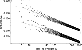
Figure 1: Dilog graphic with the simulated values of the critical level and the fitted function for k=2. Critical levels calculated with weights (a=1,b=1) are indicated by $\ocircle$, and with weights (a=4,b=1) are indicated by $+$.

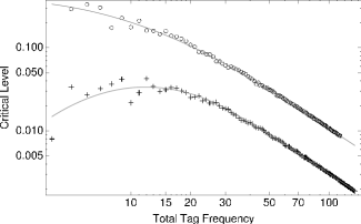
Figure 2: Dilog graphic with the simulated values of the critical level and the fitted functions for k=5. Critical levels calculated with weights (a=1,b=1) are indicated by $\ocircle$, and with weights (a=4,b=1) are indicated by $+$.

As can be seen, the set of weights (a=4,b=1) generates critical level values that are consistently lower than those obtained using the set (a=1,b=1). This result can be ascribed to weight 4 used for the $\alpha$ error, which leads to a greater minimization of type I error. Also, for both sets of weights, when y presents high values, the critical level is much more stringent than the canonical values 0.1, 0.05 and 0.01.

7.2 Comparison between Kemp p-value and $\chi^{2}$ p-value

The $\chi^{2}$ homogeneity test is widely used and described in the literature for comparison of digital expression profiles (Man et al., 2000; Romualdi et al., 2001). We decided to compare our frequentist significance level (p-value) to the $\chi^{2}$ test. We used a data set composed of four SAGE libraries derived from human brain tissues, and potentially containing genes involved in increased risk of Alzheimer’s Disease (GEO accession code GSE6677). The tags were arbitrarily separated into two groups according to their total frequency ($y$). Thus, we calculated the significance levels using the Kemp method and the $\chi^{2}$ test for both, the high-expression ($y>50$, Fig. 3) and low expression ($y\leq 50$, Fig. 4) tags. In Fig. 3, we can see that there is a good agreement between the significance levels when tags present a high expression level. Conversely, Fig. 4 shows that when the expression of the tags is relatively low, the levels present a much lower agreement. This result is in consonance with what we should expect, since the $\chi^{2}$ test is asymptotic, whereas our proposed significance test is exact.

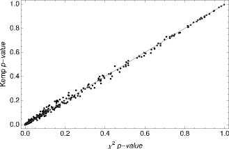
Figure 3: Relation between Kemp p-value and $\chi^{2}$ p-value for tags with $y>50$.

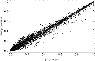
Figure 4: Relation between Kemp p-value and $\chi^{2}$ p-value for tags with $y\leq 50$

7.3 Comparison between Kemp p-value and Basu e-value

Aiming at estimating the consistency of the proposed methods, we compared the p-value (the frequentist significance level), and the e-value (the Bayesian significance level) using the four SAGE libraries described in the section 7.2. To obtain the relationship between p-values and e-values we calculated the local weighted average of the e-values, using the values of $y$ as weights and a p-value intervals of 0.04. This calculation resulted into pairs $(\bar{p},\bar{e})$, where $\bar{p}$ is the center of the interval, and $\bar{e}$ the weighted average. We then adjusted a Beta distribution function to these pairs. The best fit obtained was a Beta with parameters $a=0.66$ e $b=1.036$, corresponding to a mean of 0.39 and a standard deviation of 0.30. Fig. 5 displays a plot of the relationship between both significance levels, and the fitted function. We can notice that there is a good agreement between the p-value and e-value. Some differences observed between their values can be explained by the fact that the p-value is an integral in the sample space, whereas the e-value is an integral in the parameter space. Despite this difference, it is clear that both significance levels are most of times convergent.

Figure 5: Relationship between p-value and e-value. $\ocircle$ indicate the pairs $(\bar{p},\bar{e})$ and the curve the fitted function.

8 Discussion

This paper introduces two novel methods for the comparison of digital expression profiles. The methods, based on frequentist and Bayesian statistics, were implemented on the open source programs Kemp and Basu, respectively. Several statistical tests have been used to evaluate SAGE data and identify differentially expressed tags. Some of these tests have been compared by different groups (Man et al., 2000; Romualdi et al., 2001; Ruijter et al., 2002). The general conclusion was that the classical $\chi^{2}$ test, originally introduced by Karl Pearson (Pearson, 1900), was equivalent to and even outperformed other available tests, including the Fischer’s Exact test, the test of Audic and Claverie (1997) and the R statistic of Stekel et al. (2000). The $\chi^{2}$ test has the advantage of being simple and can be applied to a broad range of problems. However, given the asymptotic character of the $\chi^{2}$ test, it is not recommended for the analysis of low frequency tags. Due to this feature, we conceived our frequentist test using the original definition of more extreme sample points, without any asymptotic result. As a consequence, our test is more correct than the $\chi^{2}$ test for low expression tags. Corroborating this fact, a comparison of the p-values calculated by Kemp, and the $\chi^{2}$ p-value, showed a good agreement (Fig. 3 and Fig. 4) only for high expression tags. For low frequency tags, when the $\chi^{2}$ test becomes inappropriate, $\chi^{2}$ values showed a high disagreement with our calculated p-values (Fig. 4). Thus, we believe that the frequentist test proposed here, and implemented on Kemp, represents an improvement for the analysis of digital expression profiles.

Some other methods (Baggerly et al., 2004; Robinson and Smyth, 2007; Thygesen and Zwinderman, 2006; Vêncio et al., 2004) have been proposed for the comparative analysis of SAGE data. However, since these methods are designed for comparing groups of libraries, their use is severely restricted in experiments where a single library is represented in each category/condition.

The discrimination between high and low expression tags must be performed in such a way as to consider both statistical and biological relevance. Since housekeeping genes are expressed in high levels, the absolute number of counts may present a considerable variation across distinct libraries. These differences, nevertheless, are meaningless from a biological standpoint. Conversely, some functionally important genes present a relatively low expression, and exert their activity by altering tiny amounts of their expression among the different tissues and/or conditions (Wang, 2006). Therefore, a tag presenting a differential expression with low counts would not be considered as significant by methods that use fixed critical levels, thus leading to a misinterpretation of the data and loss of potentially valuable information. This fact motivated us to calculate the critical level of each particular tag taking into account its total frequency. If population parameters are not exactly in the null sharp hypothesis set (a set with a smaller dimension than the alternative hypothesis set), highly expressed tags have smaller p-values than low expression tags. If one fixes the critical level, the minimum type I error, the type II error decreases drastically when the sample size is increased. Hence, it becomes difficult to accept a null hypothesis for large sample sizes, and to reject it for small-sized samples. For example, when comparing the expression of two 10,000-tag libraries, a tag presenting counts of 7 and 21, respectively, would show a p-value of 0.013. Conversely, a tag with counts 10 and 30 would result in a p-value of 0.002. Considering a cutoff of 0.01, the former tag would be considered as equally expressed in both libraries, whereas the former tag would be interpreted as being differentially expressed. This fact motivated us to calculate the critical level of each particular tag as a function of the tag total frequency. The critical region in our method is the one that minimizes a linear combination of type I (the critical level $\alpha$) and type II ($\beta$) errors. With this tag-customized approach, both tags of the example above would be classified as differentially expressed, since their corresponding critical levels would be 0.015 and 0.013, respectively. The method is still coherent, since tags with very low frequencies, even presenting differential counts, lead to high significance levels. For instance, in the aforementioned example, tag counts of 1 and 3 would result in a p-value of 0.63, a much higher value than the calculated cutoff of 0.03. Concluding, our method judges the tags in a fairer manner, since the cutoff value is customized to any particular tag, according to its expression level.

The problem of significance testing of precise (sharp) hypotheses has been controversial and both, the frequentist and Bayesian schools of statistical inference, have offered solutions. As a counterpart to the frequentist test introduced in this work, we decided to also offer an alternative method, based on the previously described (Pereira et al., 2008) Full Bayesian Significance Test (FBST). A clear advantage of a Bayesian test, applied to digital expression profiling, is that the total frequencies of the tags do not have to be fixed in advance and are, in fact, unknown before the observation of the libraries. This Bayesian procedure does not require any other assumption in addition to the original multivariate Bernoulli observations that produce the libraries. From a Bayesian standpoint, it is important to judge hypotheses in their own environment, which is the parameter space, not the sample space. With a more pragmatic view on mind, we tried to check if the frequentist and Bayesian tests can be related, even though they are defined in different spaces. In this direction, we implemented the FBST in the Basu program, and compared the e-values to the p-values previously determined by Kemp (the frequentist test program), using SAGE libraries. To our surprise, a strong correspondence between the averages of p-values and e-values has been observed (Fig. 5). This result indicates that both methodologies can be reliably used to identify differentially expressed tags. Also, because they lead to similar results using totally different approaches, we believe that both methods can be used in parallel to validate each other’s results.

Kemp method fully implements a decision procedure, since it provides a significance level and a critical level. Conversely, Basu method does not calculate the most appropriate cutoff. For this task, one should follow the decision theory steps described by Pereira et al. (2008), and build a loss function based on a good modeling of the risks involved on deciding whether a tag should or not be considered as differentially expressed. In this direction, our group is currently working on the development of a critical level for the FBST. Alternatively, one can use an approximation to determine a cutoff for Basu. Since the p-values and e-values are linked by a Beta distribution function, as we have shown for a set of SAGE libraries from human brain tissue (Fig. 5) and some other datasets (data not shown), we propose to use the Kemp cutoff, properly adjusted by the linking function.

Concluding, the frequentist and Bayesian significance tests reported in the present work, and implemented in standalone open-source programs, extend the set of currently available statistical tests for digital expression profiles. Also, we believe that they offer some advantages over other reported tests, including a more adequate treatment of low expression tags and the automatic calculation of a customized critical level.

System Requirements

The source code of KempBasu package and a executable binary for MS Windows are publicly available at the address http://code.google.com/p/kempbasu/, and are distributed under the GNU General Public License. The code depends on glib, GSL and Judy libraries, and if the Pthreads API is available, KempBasu can be run using multiple processors. Tested platforms include Linux, MacOSX and MS Windows.

Appendix

To establish the function of y that gives the approximate $\alpha$, we consider the pairs $\{L=Log(y);Log(\alpha)\}$ and use the least squares method piecewisely in two difference regions of $y$ values: [1;50] and [51;10,000] . The former region adjusts a second degree polynomial

$$\alpha_{k}^{(1)}(y)=a_{k}L^{2}+b_{k}L+c_{k}$$

and the latter region adjusts a line

$$\alpha_{k}^{(2)}(y)=u_{k}+v_{k}L.$$

Tables 1 and 2 present the coefficient values for those functions for weights $(a=4,b=1)$ and $(a=1,b=1)$, respectively . The linear and the quadratic functions are combined, for each value of $k$, into a single continuos function by the eq. 12.

$$\alpha_{k}(y)=\left\{\begin{array}[]{ll}\alpha_{k}^{(1)}(y)&\text{para }y<40\\ (1-\lambda)\alpha_{k}^{(1)}(y)+\lambda\alpha_{K}^{(2)}(y)&\text{para }40\leq y<50\\ \alpha_{k}^{(2)}(y)&\text{para }y\geq 50\\ \end{array}\right.$$ (12)

k	$a_{k}$	$b_{k}$	$c_{k}$	$u_{k}$	$v_{k}$
2	0.00957978	-0.463118	-2.76474	-2.37781	-0.530119
3	-0.304365	1.18976	-4.60784	-0.713611	-0.968513
4	-0.931159	5.00318	-10.1863	0.385118	-1.28105
5	-0.685327	3.39467	-7.59502	1.47602	-1.57657
6	-0.914225	4.84175	-9.81444	1.93518	-1.70783

Table 1: Coefficient values of fitted critical level functions for the minimization of $4\alpha+\beta$

k	$a_{k}$	$b_{k}$	$c_{k}$	$u_{k}$	$v_{k}$
2	0.00748022	-0.607463	-0.53588	-0.629139	-0.561742
3	-0.226299	0.503742	-1.7504	0.677628	-0.968169
4	-0.215143	0.334093	-1.38061	1.79399	-1.30545
5	-0.248689	0.369967	-1.13529	2.62984	-1.55664

Table 2: Coefficient values of fitted critical level functions for the minimization of $\alpha+\beta$

References

- Aitchison (2003) Aitchison,J. (2003). The Statistical Analysis of Compositional Data. Chapter 6. Blackburn Press, New Jersey, pp. 126–128.
- Audic and Claverie (1997) Audic,S. and Claverie,J.M. (1997). The significance of digital gene expression profiles. Genome Res., 7, 986–95.
- Baggerly et al. (2004) Baggerly,K., Deng,L., Morris,J., and Aldaz,C. (2004). Overdispersed logistic regression for SAGE: Modelling multiple groups and covariates. BMC Bioinformatics, 5, 144.
- Basu (1977) Basu,D. (1977). On the elimination of nuisance parameters. J. Am. Stat. Assoc., 72, 355–366.
- Brenner et al. (2000) Brenner,S.E., Johnson,M., Bridgham,J., Golda,G., Lloyd,D., Johnson,D., Luo,S., McCurdy,S., Foy,M., Ewan,M., et al. (2000). Gene expression analysis by massively parallel signature sequencing (MPSS) on microbead arrays. Nat. Biotechnol., 18, 630–634.
- Cai et al. (2004) Cai,L., Huang,H., Blackshaw,S., Liu,J.S., Cepko,C., and Wong,W.H. (2004). Clustering analysis of SAGE data using a Poisson approach. Genome Biol., 5, R51.
- Cox (1975) Cox,D. (1975). Partial likelihood. Biometrika, 62, 269–276.
- Cox (1977) Cox,D. (1977). The role of significant test (with discussion). Scand. J. Statist., 4, 49–70.
- DeGroot (1986) DeGroot,M.H. (1986). Probability and statistics. Addison-Wesley, Boston.
- Dempster (1997) Dempster,A.P. (1997). The direct use of likelihood for significance testing. Stat. Comput., 7, 247–252.
- Kempthorne (1976) Kempthorne,O. (1976). Of what use are tests of significance and tests of hypothesis. Commun. Stat. A-Theor., 5, 763–777.
- Kempthorne and Folks (1971) Kempthorne,O. and Folks,L. (1971). Probability, Statistics and Data Analysis. Iowa State University Press, Ames.
- Man et al. (2000) Man,M.Z., Wang,X., and Wang,Y. (2000). POWER_SAGE: comparing statistical tests for SAGE experiments. Bioinformatics, 16, 953–9.
- Neyman and Pearson (1928) Neyman,J. and Pearson,E.S. (1928). On the use and interpretation of certain test criteria for purposes of statistical inference: Part I. Biometrika, 20, 175–240.
- Pearson (1900) Pearson, K. (1900). On the criterion that a given system of deviations from the probable in the case of a correlated system of variables is such that it can be reasonable supposed to have arisen from random sampling. Philos. Mag., 50, 157–175.
- Pereira and Stern (1999) Pereira,C.A.B. and Stern,J.M. (1999). Evidence and credibility: full bayesian significance test for precise hypotheses. Entropy, 1, 99–110.
- Pereira and Wechsler (1993) Pereira, C. A. B. and Wechsler, S. (1993). On the concept of p-value. Braz. J. Prob. Statist, 7, 159–177.
- Pereira et al. (2008) Pereira,C.A.B., Stern,J.M., and Wechsler,S. (2008). Can a significance test be genuinely Bayesian? Bayesian Anal., 3, 79–100.
- Robinson and Smyth (2007) Robinson,M. and Smyth,G. (2007). Small-sample estimation of negative binomial dispersion, with applications to SAGE data. Biostatistics, 9, 321–332.
- Romualdi et al. (2001) Romualdi,C., Bortoluzzi,S., and Danieli,G. (2001). Detecting differentially expressed genes in multiple tag sampling experiments: comparative evaluation of statistical tests. Hum. Mol. Genet., 10, 2133–2141.
- Ruijter et al. (2002) Ruijter,J., Van Kampen,A., and Baas,F. (2002). Statistical evaluation of SAGE libraries: consequences for experimental design. Physiol. Genomics, 11, 37–44.
- Stekel et al. (2000) Stekel,D.J., Git,Y., and Falciani,F. (2000). The comparison of gene expression from multiple cDNA libraries. Genome Res., 10, 2055–2061.
- Stollberg et al. (2000) Stollberg,J., Urschitz, J.,Urban,Z., and Boyd,C.D. (2000). A quantitative evaluation of SAGE. Genome Res., 10, 1241–1248.
- Thygesen and Zwinderman (2006) Thygesen,H.H. and Zwinderman,A.H. (2006). Modeling SAGE data with a truncated gamma-poisson model. BMC Bioinformatics, 7, 157.
- Velculescu et al. (1995) Velculescu,V.E., Zhang,L., Vogelstein,B., and Kinzler,K.W. (1995). Serial analysis of gene expression. Science, 270, 484–487.
- Vêncio et al. (2004) Vêncio,R.Z.N., Brentani,H., Patrão,D.F.C., and Pereira,C.A.B. (2004). Bayesian model accounting for within-class biological variability in serial analysis of gene expression (SAGE). BMC Bioinformatics, 5, 119.
- Wang (2006) Wang,S. (2006). Understanding SAGE data. Trends in Genet., 23, 42–50.
- Zhu et al. (2008) Zhu,J., He,F., Wang,J., and Yu,J. (2008). Modeling transcriptome based on transcript-sampling data. PLoS ONE, 3, e1659.