Exploring the magnetized cosmic web through low frequency radio emission

Abstract

Recent improvements in the capabilities of low frequency radio telescopes provide a unique opportunity to study thermal and non-thermal properties of the cosmic web. We argue that the diffuse, polarized emission from giant radio relics traces structure formation shock waves and illuminates the large-scale magnetic field. To show this, we model the population of shock-accelerated relativistic electrons in high-resolution cosmological simulations of galaxy clusters and calculate the resulting radio synchrotron emission. We find that individual shock waves correspond to localized peaks in the radio surface brightness map which enables us to measure Mach numbers for these shocks. We show that the luminosities and number counts of the relics strongly depend on the magnetic field properties, the cluster mass and dynamical state. By suitably combining different cluster data, including Faraday rotation measures, we are able to constrain some macroscopic parameters of the plasma at the structure formation shocks, such as models of turbulence. We also predict upper limits for the properties of the warm-hot intergalactic medium, such as its temperature and density. We predict that the current generation of radio telescopes (LOFAR, GMRT, MWA, LWA) have the potential to discover a substantially larger sample of radio relics, with multiple relics expected for each violently merging cluster. Future experiments (SKA) should enable us to further probe the macroscopic parameters of plasma physics in clusters.

1 Introduction and key questions

The plasma within and between galaxies is magnetized. Despite many observational efforts to measure galactic and intergalactic magnetic fields, their properties and origins are not currently well understood. The magnetic fields influence the physics of the plasma in several important ways. They couple the collisionless charged particles to a single but complex fluid through the Lorentz force, and trace dynamical processes in the Universe. Magnetic pressure and tension mediate forces and provide the plasma with additional macroscopic degrees of freedom in terms of Alfvénic and magnetosonic waves. They cause the turbulent cascade to become anisotropic towards smaller scales and suppress transport processes such as heat conduction and cosmic ray diffusion across the mean magnetic field. They are essential for accelerating cosmic rays by providing macroscopic scattering agents which enables diffusive shock acceleration (first order Fermi process) and through magneto-hydrodynamic turbulent interactions with cosmic rays leading to second order Fermi acceleration. They illuminate distant cosmic ray electron populations by enabling synchrotron emission and tell us indirectly about violent high-energy astrophysical processes such as formation shock waves or $\gamma$-ray bursts. The magnetic fields in spiral galaxies are highly regular, showing alignment with the spiral arms. They are believed to arise from weak seed fields amplified by dynamo processes, driven by differential rotation in galactic disks. The seed fields could have been produced by many sources, ranging from stellar winds and jets of active galactic nuclei, to plasma instabilities and battery effects in shock waves, in ionization fronts, and in neutral gas-plasma interactions. More hypothetical ideas for the seed field origins invoke primordial generation in early Universe processes, such as phase transitions during the epoch of inflation. In order to understand more about magneto-genesis, we need to study the least processed plasma possible that still shows some primordial memory. This points us to the magnetized plasma in intergalactic space, in particular to the plasma in galaxy clusters. There, magnetic fields show a smaller degree of ordering compared to spiral galaxies. However, their primordial properties may be masked in clusters because of processing by turbulent gas flows, driven by galaxy cluster mergers, and the orbits of the member galaxies. For an overview on the present observational and theoretical knowledge the reader is pointed to the review articles by Rees (1987); Wielebinski & Krause (1993); Kronberg (1994); Beck et al. (1996); Kulsrud (1999); Beck (2001); Grasso & Rubinstein (2001); Carilli & Taylor (2002); Widrow (2002). This work aims at closing a gap between theoretically motivated phenomenological models of large scale magnetic fields and actual observational non-thermal phenomena associated with them.

Diffuse radio synchrotron emission has already been observed in more than 50 galaxy clusters (Ferrari et al., 2008). The emission is associated with the entire intra-cluster medium (ICM). The synchrotron emission process demonstrates the presence of highly relativistic electrons (cosmic ray electrons, CRe) with a Lorentz factor typically up to $\gamma\sim 10^{4}$ and magnetic fields within the ICM. The diffuse radio emission can be classified into two categories: radio halos and radio relics. Giant radio halos are centrally located, trace the thermal emission and show no sign of polarization, while radio relics are located at the periphery of clusters, are polarized and are elongated in appearance. There exist a number of classes of radio objects that have been referred to over the years as “radio relics” (Kempner et al., 2004, and references therein). Two of these are associated with extinct or dying active galactic nuclei (AGN). These either host a synchrotron cooling radio plasma from a past AGN outburst that created the radio lobes or are revived “radio ghosts” where an aged radio relic has been re-energized by a merger or an accretion shock (Enßlin & Gopal-Krishna, 2001).

The focus of this paper is on a third type of radio relic emission, sometimes referred to as radio “gischt” (Kempner et al., 2004), that shows diffuse emission on scales up to 1 Mpc. Diffusive shock acceleration at structure formation shocks can energize a primary population of relativistic electrons that emit synchrotron radiation (Enßlin et al., 1998; Miniati et al., 2001) in a magnetic field that can be amplified by the post-shock turbulence. Prominent examples for this class of radio relics can be seen in Abell 3667 (Röttgering et al., 1997), Abell 2256 (Bridle & Fomalont, 1976; Masson & Mayer, 1978; Bridle et al., 1979; Röttgering et al., 1994; Clarke & Enßlin, 2006), Abell 3376 (Bagchi et al., 2006), and, more recently, Abell 2255 (Pizzo et al., 2008) and Abell 521 (Giacintucci et al., 2008). All galaxy clusters with observed radio relic emission are merging or show signs of ongoing dynamical activity, but not all dynamically active galaxy clusters are observed to have relics. This raises the question of whether diffuse radio emission is a property of a special subset of clusters, or a universal property, with many relics too faint to be seen by current telescopes.

From CMB measurements we know that the Universe is composed of 4.6% baryonic matter, e.g. Komatsu et al. (2008). However, when observing the local Universe ($z<1$), we can account for fewer than half of these baryons (Fukugita, 2004; Danforth & Shull, 2005). This is known as the missing baryon problem. The current cosmological paradigm of large scale structure formation provides a solution to the missing baryon problem. As the Universe evolves, large scale structure grows from small density perturbations imprinted during an earlier epoch. In the hierarchical scenario of structure formation, structure grows from small to large scales, with baryons flowing in a filamentary web with clusters at the interstices. The temperature of baryons deviates from adiabatic cooling associated with the Hubble expansion by increasing multiple times in discrete steps – always corresponding to a passage through a structure formation shock. Before they are shock-heated to the virial temperatures $kT\sim 1-10$ keV of galaxy groups and clusters, where they can be observed through their thermal bremsstrahlung emission, they are predicted to reside in the warm-hot intergalactic medium (WHIM). Temperatures in the WHIM are in the range of $10^{5}\,\mbox{K}<T<10^{7}\,\mbox{K}$ (Hellsten et al., 1998; Cen & Ostriker, 1999; Davé et al., 2001; Furlanetto & Loeb, 2004; Kang et al., 2005). We will investigate whether it is possible for diffuse radio emission associated with these formation shocks to be used as a tracer of the WHIM boundaries and so indirectly observe the WHIM.

Mach numbers

Radio Gischt at shocks

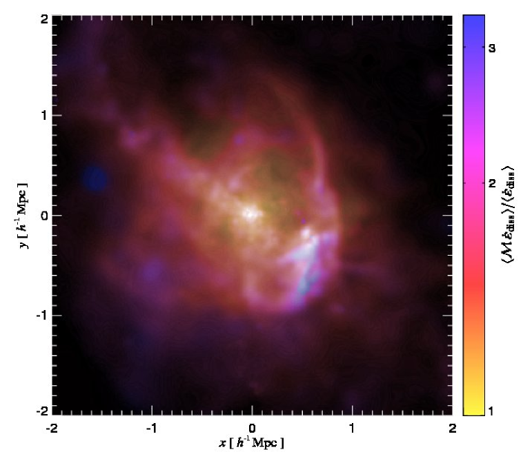
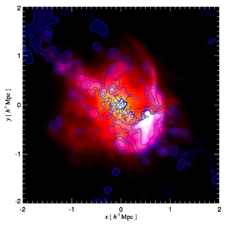
Figure 1: Structure formation shocks triggered by a recent merger of a large galaxy cluster ($M\simeq 10^{15}h^{-1}\,\mathrm{M}_{\odot}$) dissipate the associated gravitational energy. Left: the Mach number of shocks weighted by the energy dissipation rate is shown by the colour (while the brightness displays the logarithm of the dissipation rate). Right: three-color image of energy dissipation rate at shocks (shown with a color scale ranging from black over red to yellow) and radio synchrotron emission at 150 MHz from shock-accelerated relativistic electrons (blue and contours with levels starting at $7\times 10^{-4}$ mJy arcmin^-2 and increasing with a factor of 15, respectively). This “radio gischt” emission traces structure formation shock waves, highlights the intermittent nature of mass accretion in galaxy clusters, and illuminates magnetic fields that are amplified by turbulence that can be excited by these shock waves.

A larger sample size of these diffuse radio sources is required to delve deep into the details of the non-thermal processes working within galaxy clusters. However, the combination of low surface brightness, diffuseness and small dynamical range in the sensitivity of current radio telescopes makes the detection of this particular radio emission difficult. With the current capabilities of the Giant Meter Radio Telescope (GMRT, Ananthakrishnan 1995) and the imminent arrivals of the Low Frequency ARray (LOFAR, Röttgering 2003), the Murchison Wide-field Array (MWA, Morales et al. 2006) and the Long Wavelength Array (LWA, Kassim et al. 2005), and eventually the construction of the Square Kilometre Array (SKA, Keshet et al. 2004b), powerful low frequency radio telescopes are positioned to further increase our understanding of diffuse radio emission and give us insight into the following important topics:

• the strength and coherence scale of magnetic fields on scales of galaxy clusters,

• the process of diffusive shock acceleration of electrons,

• the existence and properties of the WHIM,

• the exploration of observables beyond the thermal cluster emission which are sensitive to the dynamical state of the cluster.

In the course of this work we will consider how radio relic emission can shed light on each of these topics. To do this, we adopt a simplified model for the shock-accelerated population of electrons. The key figure illustrating these considerations is shown in Fig. 1. In our simulations, we can visualize properties of structure formation shocks that are triggered by a recent merger of a large galaxy cluster ($M\simeq 10^{15}h^{-1}\,\mathrm{M}_{\odot}$) and dissipate the associated gravitational energy. In the left panel, the shock Mach numbers, weighted by the energy dissipation rate, are encoded by the colour, while the brightness displays the logarithm of the dissipation rate. This shows that most of the energy is dissipated in weak flow shocks internal to the cluster, while the shock waves become strongest and steepen as they break at the shallower peripheral potentials of the clusters and within filaments. The right panel shows a three-color image of of energy dissipation rate at shocks (shown in red and yellow) and radio synchrotron emission at 150 MHz from shock-accelerated relativistic electrons (blue and contours, modeled according to Pfrommer et al. 2008). This “radio gischt” emission traces structure formation shock waves and highlights the intermittent nature of mass accretion, in particular along the filament extending from the cluster center to the upper left of the image and for the giant radio relic to the lower-right of the cluster. This radio emission illuminates magnetic fields that are amplified by magneto-hydrodynamic instabilities that are associated with these shock waves. The paper has been structured accordingly: in Sect. 2 we outline our methodology; we describe our results and discuss them in Sects. 3 and 4; and present our conclusions in Sect. 5.

2 Methodology

We briefly summarize our procedure. We model the synchrotron emission by calculating the primary shock-accelerated electron population using a scheme that is based on the thermal leakage model – a model that has been developed in the context of diffusive shock acceleration at supernova remnants (Ellison et al., 1981). We use a simple parametrization for the magnetic field. This lets us quickly scan the observationally allowed parameter space associated with the mostly-unknown spatial distribution of shocks on cluster scales and beyond. In the post-processing, we search for spatially correlated synchrotron emission from formation shocks, which represent our simulated radio relics and study the properties of these relics in the clusters in our sample. Our aim is to understand how radio observables can be used to reconstruct the physical properties of radio relics, which trace structure formation and large scale magnetic fields. In the subsequent sections there will be a detailed description of our simulations and modelling.

Observable parameters

Theoretical parameters

Total emission

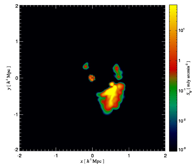
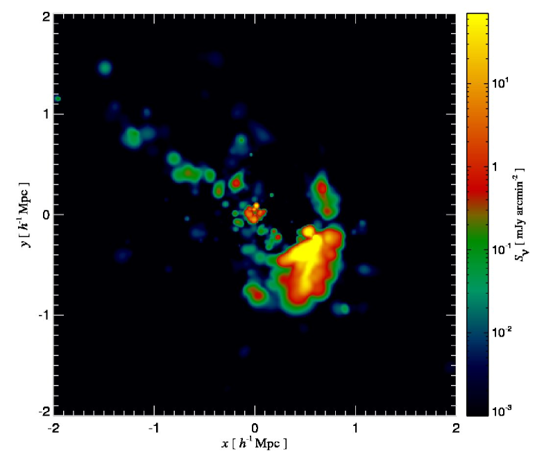
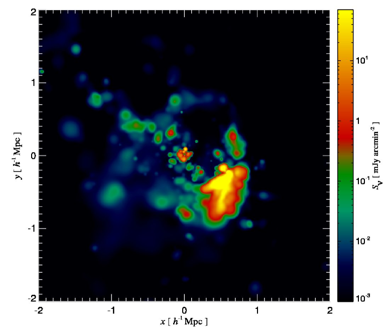
Figure 2: Surface brightness emission map for radio relics in the simulated cluster g72a Left to right: the emission from two sets of relic finder parameters, and the total primary radio emission at 150 MHz. Our relic finder groups SPH particles using a friends-of-friends algorithm; we additionally require these particles to exceed a emissivity threshold (ET). The differences in the images illustrate the dependence on ET (left panel: observable parameters with ET = $10^{-43}$ $h^{3}$ erg s^-1 Hz^-1 ster^-1 cm^-3, central panel: theoretical parameters ET = $10^{-55}$ $h^{3}$ erg s^-1 Hz^-1 ster^-1 cm^-3). The central map only lacks surface brightness at the level of $10^{-3}$ compared to the total primary emission. Both relic emission maps to the left contain more than 99% of the total flux from the total primary emission map.

2.1 Adopted cosmology and simulated cluster sample

Our work is based on high resolution smoothed particle hydrodynamics (SPH) simulations of galaxy clusters (minimum gas mass resolution $\sim 8\times 10^{9}h^{-1}\mathrm{M}_{\sun}$ for more details, cf. Pfrommer et al., 2007, 2008) using the ‘zoomed initial conditions’ technique (Katz & White, 1993) that were selected from a low resolution dark matter only simulation (Yoshida et al., 2001) with a box size of 479 $h^{-1}$ Mpc. They were carried out using a modified version of the massively parallel tree SPH code GADGET-2 (Springel, 2005). The simulations of the galaxy clusters were performed in a “Concordance” cosmology model, $\Lambda$CDM with cosmological parameters of: $\Omega_{\mathrm{m}}$= $\Omega_{\mathrm{DM}}$ + $\Omega_{\mathrm{b}}$ = 0.3, $\Omega_{\mathrm{b}}$ = 0.039, $\Omega_{\Lambda}$ = 0.7, $h$ = 0.7, $n_{s}$ = 1 and $\sigma_{8}$ = 0.9. Here, $\Omega_{\mathrm{m}}$ refers to the total matter density in units of the critical density today, $\rho_{\mathrm{crit}}=3H_{0}^{2}/(8\pi G)$. $\Omega_{\mathrm{b}}$ and $\Omega_{\Lambda}$ denote the densities of baryons and the cosmological constant at the present day. The Hubble constant at the present day is parametrized as $H_{0}=100\,h\mbox{ km s}^{-1}\mbox{Mpc}^{-1}$, while $n_{s}$ denotes the spectral index of the primordial power-spectrum, and $\sigma_{8}$ is the rms linear mass fluctuation within a sphere of radius $8\,h^{-1}$Mpc extrapolated to $z=0$.

The simulations include a prescription for radiative cooling, star formation, supernova feedback and a formalism for detecting structure formation shocks and measuring the associated shock strengths, i.e. the Mach numbers (Pfrommer et al., 2006). Radiative cooling was computed assuming an optically thin gas of primordial composition (mass-fraction of $X_{\mathrm{H}}=0.76$ for hydrogen and $1-X_{\mathrm{H}}=0.24$ for helium) in collisional ionisation equilibrium, following Katz et al. (1996). We also included heating by a photo-ionising, time-dependent, uniform ultraviolet (UV) background expected from a population of quasars (Haardt & Madau, 1996), which reionises the Universe at $z\simeq 6$. Star formation is treated using the hybrid multiphase model for the interstellar medium introduced by Springel & Hernquist (2003). In short, the ISM is pictured as a two-phase fluid consisting of cold clouds that are embedded at pressure equilibrium in an ambient hot medium.

The cluster sample is displayed in Table LABEL:tab:cluster. From this sample the cluster g72a was chosen for detailed analysis of the properties of radio relics since it is a relatively large (with a mass $M\simeq 10^{15}\mathrm{M}_{\odot}$) post-merging cluster, similar to the Coma cluster. Additionally, it hosts the brightest radio relic in the entire sample. This relic resembles already observed ones.

Table 1: Cluster sample considered in this paper.

cluster	dynamical	$M_{200}^{b}$	$R_{200}^{b}$	$kT_{200}^{c}$
name	statea	[$h^{-1}\mathrm{M}_{\sun}$]	[$h^{-1}$ Mpc]	[keV]
g8a	CC	$1.8\times 10^{15}$	2.0	13.1
g1a	CC	$1.3\times 10^{15}$	1.8	10.6
g72a	PostM	$1.1\times 10^{15}$	1.7	9.4
g51	CC	$1.1\times 10^{15}$	1.7	9.4
g1b	M	$3.7\times 10^{14}$	1.2	4.7
g72b	M	$1.5\times 10^{14}$	0.87	2.4
g1c	M	$1.4\times 10^{14}$	0.84	2.3
g1d	M	$9.2\times 10^{13}$	0.73	1.7
g676	CC	$8.8\times 10^{13}$	0.72	1.7
g914	CC	$8.5\times 10^{13}$	0.71	1.6

^a The dynamical state has been classified through a combined criterion invoking a merger tree study and the visual inspection of the X-ray brightness maps. The labels for the clusters are M–merger, PostM–post merger (slightly elongated X-ray contours, weak cool core region developing), CC–cool core cluster with extended cooling region (smooth X-ray profile). ^b The virial mass and radius are related by $M_{\Delta}(z)=\frac{4}{3}\pi\,\Delta\,\rho_{\mathrm{crit}}(z)R_{\Delta}^{3}$, where $\Delta=200$ denotes a multiple of the critical overdensity $\rho_{\mathrm{crit}}(z)=3H(z)^{2}/(8\pi G)$. ^c The virial temperature is defined by $kT_{\Delta}=GM_{\Delta}\,\mu\,m_{\rm p}/(2R_{\Delta})$, where $\mu$ denotes the mean molecular weight.

2.2 Realization of magnetic fields

Current SPH implementations that are capable of following the magneto-hydrodynamics (MHD) of the gas are presently still fraught with numerical and physical difficulties, in particular when following dissipative gas physics (Dolag et al., 1999; Dolag et al., 2005; Price & Monaghan, 2004, 2005). Hence we apply a parametrization in the post-processing of our completed simulations in order to determine the strength and morphology of the magnetic field (Pfrommer, 2008). Secondly, the parametrization approach provides us with the advantage of exploring the parameter space of our magnetic field description more efficiently, since we are not required to re-simulate when we alter the ab-initio unknown magnetic field parameters. We have chosen a simple scaling model for the magnetic field of

$$\varepsilon_{B}=\varepsilon_{B_{0}}\left(\frac{\varepsilon_{\mathrm{th}}}{\varepsilon_{\mathrm{th}_{0}}}\right)^{2\alpha_{B}}.$$ (1)

Our independent model parameters are the magnetic decline $\alpha_{B}$, and the magnetic core energy density $\varepsilon_{B_{0}}$. The thermal energy density $\varepsilon_{\mathrm{th}}$ is measured in units of its central energy density $\varepsilon_{\mathrm{th_{0}}}=3P_{\mathrm{th}_{0}}/2$, which we calculate by fitting a modified $\beta$-model (Eqn. 2) to the radial pressure profiles of our clusters. We first remove the over-cooled core (see Sect. 2.4.2),

$$P(r)=P_{\mathrm{th}_{0}}\left(1+\left(\frac{r}{r_{c}}\right)\right)^{-3\beta}.$$ (2)

We found that our modified $\beta$-model provides a better fit to the pressure profiles than the usually adopted spherically symmetric King profiles, i.e. a $\beta$-model (Cavaliere & Fusco-Femiano, 1978).

This parametrization (Eqn. 1) was motivated by non-radiative SPH MHD simulations (Dolag et al., 1999) and radiative adaptive mesh refinement MHD simulations (Dubois & Teyssier, 2008) of the formation of galaxy clusters in a cosmological setting. Rather than applying a scaling with the gas density as those simulations suggest, we chose the energy density of the thermal gas. Current cosmological radiative simulations (that do not include feedback from AGN) over-cool the centres of clusters, giving an overproduction of stars, enhanced central gas densities, and lower central temperatures than are seen in X-ray observations. In contrast, the thermal energy density of the gas is well-behaved in simulations. Observationally, the parametrization (Eqn. 1) is consistent with statistical studies of Faraday rotation measure maps (Vogt & Enßlin, 2005). Theoretically, the growth of magnetic field strength is determined through turbulent dynamo processes that will saturate at a field strength determined by the strength of the magnetic back-reaction (e.g. Subramanian, 2003; Schekochihin & Cowley, 2006) and is typically a fraction of the turbulent energy density. The turbulent energy density should be related to the thermal energy density, thus motivating our model theoretically. The parameter $\varepsilon_{B_{0}}$ is constrained by past measurements of magnetic fields within clusters and is chosen such that $B_{0}=[\varepsilon_{B_{0}}8\pi]^{1/2}$ to be on the order of a few $\mu$G (Govoni et al., 2006; Taylor et al., 2007; Guidetti et al., 2008). The parameters explored in our model are shown in Table LABEL:tab:bpar.

Table 2: Magnetic field parameters in various combinations. We define our standard magnetic field parameters to be $\alpha_{B}$ = 0.5, $B_{0}$ = 5$\mu$G and $\nu$ = 150MHz. These parameters are used throughout the paper unless otherwise stated.

$\alpha_{B}$	$B_{0}$ [$\mu$G]
magnetic decline	core magnetic field strength
0.3	2.5
0.5	5.0
0.7	10.0
0.9	-

To predict the polarization angle and Faraday rotation measure in our simulations, we need to model the magnetic morphology of the ICM. We follow Tribble (1991) in order to create individual components of the magnetic vector field that obey a given power spectrum. The details of the magnetic field structure within the ICM are still unknown. There have been measurements of magnetic correlations from Faraday rotation measure (RM) maps which are however limited by the finite window size of radio lobes and hence only constrain the spectrum on smaller scales. These measurements suggest that the fields are tangled with a Kolmogorov/Oboukhov-type power spectrum for coherence lengths of approximately 10 kpc scales and smaller (Vogt & Enßlin, 2003, 2005; Guidetti et al., 2008). It has been argued that shallower magnetic field power spectra allow for longer coherence lengths on the order $100$ kpc (Murgia et al., 2004; Govoni et al., 2006). On the other hand, a Fourier analysis of XMM-Newton X-ray data reveals the presence of a scale-invariant pressure fluctuation spectrum in the range between 40 and 90 kpc and is found to be well described by a projected Kolmogorov/Oboukhov-type turbulence spectrum (Schuecker et al., 2004). Assuming that the growth of the magnetic field strength is determined through turbulent dynamo processes suggests a similar spectrum of magnetic and hydrodynamic turbulence (e.g. Subramanian, 2003).

We model the components of the magnetic field, $B_{i}$, as random Gaussian fields. We use a Kolmogorov power spectrum on scales smaller than the coherence length, and a flat (white-noise) power spectrum on larger scales. All three components of the magnetic field are treated independently, which ensures that the final distribution of $\textbf{{B}}(\textbf{{r}})$ has random phases. After mapping our SPH Lagrangian energy density distribution of the thermal gas onto a 3D grid (cf. Appendix Eqn. 23), these realizations of the magnetic field are then scaled such that the magnetic energy density obeys our assumed scaling given by Eqn. 1. To ensure $\nabla\cdot\textbf{{B}}=0$, we apply a divergence cleaning procedure to our fields in Fourier space (Balsara, 1998):

$$\tilde{B}_{i}(\textbf{{k}})=\sum_{j=1}^{3}\left(\delta_{i,j}-\frac{k_{i}k_{j}}{k^{2}}\right)\tilde{B}_{j}(\textbf{{k}}).$$ (3)

Applying this procedure to our Gaussian random field removes a third of the magnetic energy. Thus, we re-normalize B to conserve the magnetic energy.

2.3 Cosmic ray electrons and synchrotron emission

Collisionless cluster shocks are able to accelerate ions and electrons in the high-energy tail of their Maxwellian distribution functions through diffusive shock acceleration (for reviews see Drury, 1983; Blandford & Eichler, 1987; Malkov & O’C Drury, 2001). Neglecting non-linear shock acceleration and cosmic ray modified shock structure, the process of diffusive shock acceleration uniquely determines the spectrum of the freshly injected relativistic electron population in the post-shock region that cools and finally diminishes as a result of loss processes. The radio synchrotron emitting electron population cools on such a short time scale $\tau_{\mathrm{sync}}<10^{8}$ yrs (compared to the very long dynamical time scale $\tau_{\mathrm{dyn}}\sim 1$ Gyr) that we can describe this by instantaneous cooling. In this approximation, there is no steady-state electron population and we would have to convert the energy from the electrons to inverse Compton (IC) and synchrotron radiation. Instead, we introduce a virtual electron population that lives in the SPH-broadened shock volume only; this is defined to be the volume where energy dissipation takes place. Within this volume, which is co-moving with the shock, we can use the steady-state solution for the distribution function of relativistic electrons and we assume no relativistic electrons in the post-shock volume, where no energy dissipation occurs. Thus, the cooled CR electron equilibrium spectrum can be derived from balancing the shock injection with the IC/synchrotron cooling: above a GeV it is given by

$$f_{\rm e}(E)=C_{\rm e}\,E^{-\alpha_{\rm e}},\quad C_{\rm e}\propto\frac{\rho}{\varepsilon_{B}+\varepsilon_{\mathrm{ph}}}$$ (4)

Here, $\alpha_{\rm e}=\alpha_{\rm inj}+1$ is the spectral index of the equilibrium electron spectrum and $\varepsilon_{\mathrm{ph}}$ denotes the photon energy density, taken to be that of CMB photons. A more detailed description of our approach can be found in Pfrommer (2008). The synchrotron emissivity $j_{\nu}$ for a power-law spectrum of CRes scales as

$$j_{\nu}\propto C_{{\rm e}}B^{\alpha_{\nu}+1}\nu^{-\alpha_{\nu}},$$ (5)

where $\alpha_{\nu}=(\alpha_{\mathrm{e}}-1)/2$. A line-of-sight summation of $j_{\nu}$ yields the radio surface brightness, $S_{\nu}$. The surface brightness are provided in units of $h=0.7$ to simplify comparison with observations.

2.4 Finding radio relics

Dirty map

Clean map

Observable parameters

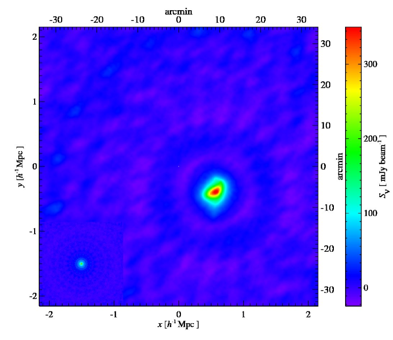
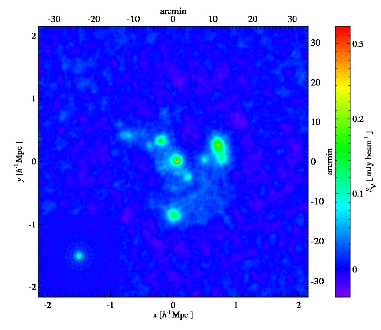
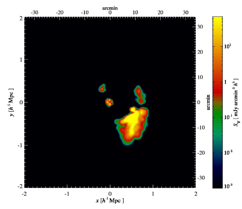
Figure 3: Left two panels: simulated GMRT map of the cluster g72a at z=0.05 (similar to the Coma cluster), with the reconstructed beam in the bottom-left corner. The left panel is the ’dirty’ map and the right panel is the ’clean’ map, where we removed the brightest relic found in the dirty map, mimicking the cleaning procedure of radio maps. Right panel: surface emission map of the relics of g72a using our calibrated set of observable parameters shown with a logarithmic colour scale. Note that we reproduce the relic emission that can principally be detected by GMRT after applying a cleaning procedure to the compact and diffuse radio emitting sources.

In our search for radio relics in the simulated clusters, we have modified a friends-of-friends (FOF) (Geller & Huchra, 1983) algorithm so that it groups together connected radio synchrotron emission in 3D. This relic finder works in a manner similar to a FOF finder except we have introduced the additional criterion of an emission threshold which the SPH gas particle are required to exceed before being assigned into a group. Thus, our algorithm depends on three internal parameters which determine the groups of particles that are designated relics: the linking length, emissivity threshold, and minimum number of particles (Fig. 2). The linking length (LL) is the parameter which controls the maximum distance ($d_{\mathrm{max}}$) between two particles that can still be considered neighbours,

$$d_{\mathrm{max}}=LL\left[\frac{\langle M_{\mathrm{DM}}\rangle}{\Omega_{\mathrm{DM}}\,\rho_{\mathrm{crit}}}\right]^{1/3},$$ (6)

where $\rho_{\mathrm{DM}}=\rho_{\mathrm{crit}}\Omega_{\mathrm{DM}}$ is the mass density of dark matter and $\langle M_{\mathrm{DM}}\rangle$ is the average mass of our dark matter particles. The linking length and the emission threshold parameters have degenerate effects on the resulting groups of particles. Through inspection, we have chosen to fix the linking length value of 0.2 resulting in $d_{\mathrm{max}}=50$ kpc and vary the emission threshold. A minimum particle value of 32 regulates possible SPH shot noise and allows for smaller structures to be included in the relic catalogue. The final parameter in our relic finder, which we have chosen to vary is the emission threshold. We compute the synchrotron emissivity of all the particles using Eqn. 5 and compare it to the emission threshold. The sets of grouped particles for each of our clusters are our relic catalogues that form the basis of our study.

2.4.1 Determination of the emission threshold

We tailored the calibration of the emission threshold in the relic finder to two cases: firstly, so that we would find relics observable by GMRT and LOFAR; secondly, so that we could study the complete picture that might be achievable with future radio telescopes such as SKA, by pushing the emission threshold back to the limit of our simulations. For this procedure, we left the magnetic field parameters unchanged. (We used our standard magnetic field parameters cf. Table LABEL:tab:bpar.)

We simulate the visibilities and maps from the relics that GMRT would observe. We use the GMRT primary beam and antenna positions projected against the zenith (i.e. ignoring the z-component of the antenna positions). For simplicity, we approximate the continuous UV tracks for each baseline by circles in the UV plane with measurements 18${\degr}$ apart. We observe cluster g72a surface emission at a redshift of 0.05 (cf. Fig. 3) and make a ‘dirty’ radio map, the Fourier transform of the visibilities. We used an integration time of 2.5 minutes with a sensitivity of 0.2 $\mathrm{mJy}\sqrt{\mathrm{hr}}/\mathrm{beam}$ at the frequency $\nu=150$ MHz in simulating the visibilities.

To approximate GMRT’s dynamical range, we modelled a simple cleaning procedure by removing the brightest relic in the ’dirty’ map from the total surface emission map and re-simulated the GMRT detections – resulting in our ‘cleaned’ radio map. We compared these maps to surface brightness maps of different relic catalogues where we varied our emission threshold (cf. Fig. 3). The emission threshold which reproduced the simulated images most accurately was $10^{-43}$ $h^{3}$ erg s^-1 Hz^-1 ster^-1 cm^-3 with the linking length and minimum number of particles already fixed. These parameters are referred throughout this paper as observable parameters.

The choice of a second emission threshold is related to the peak of the emissivity distribution function which is determined by the mass resolution of the SPH particles in the simulations. We found the peak emissivity to be at $j_{\nu}$ = $10^{-55}$ $h^{3}$ erg s^-1 Hz^-1 ster^-1 cm^-3. We find that changing $j_{\nu}$ by six orders of magnitude does not change the number of relics in a significant way (cf. Appendix B), making the difference between peak emissivity and the observable parameters reasonable. Together with the linking length and minimum number of particle parameters stated above, these parameters are referred to as theoretical parameters. Since the emissivity scales with frequency, the emission threshold must scale with frequency as well. The emission threshold (ET) scaling is fixed at our reference frequency $\nu_{0}=150$ MHz,

$$ET=ET_{0}\left(\frac{\nu}{\nu_{0}}\right)^{-1},$$ (7)

and $ET_{0}$ adopts the values quoted above for both observational and theoretical parameters.

In summary, the observable parameters were chosen to produce relic catalogues resembling the ones obtainable from current or near future observations, whereas the theoretical parameters lead to hypothetical catalogues only obtainable with a perfect 3-d tomography of the medium which may find application with the future radio interferometer SKA (cf. Table LABEL:tab:emis).

Table 3: Parameters chosen for the relic finder.

parameter	linking	minimum number	emission threshold
name	length	of particles	[erg s-1 Hz-1 ster-1 cm-3]
observable	0.2	32	10-55
theoretical	0.2	32	10-43

Observable parameters

Theoretical parameters

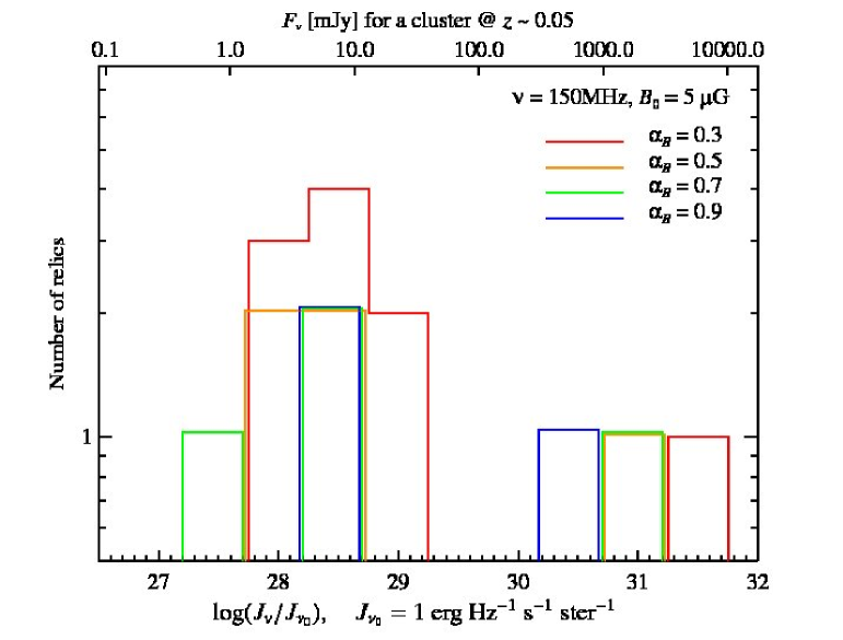
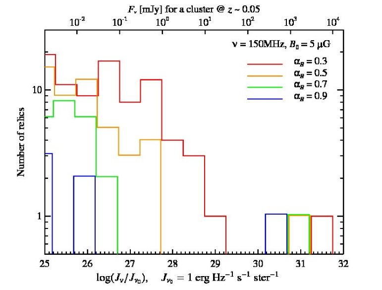
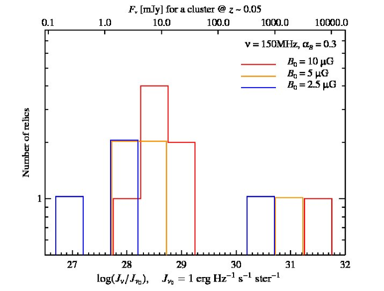
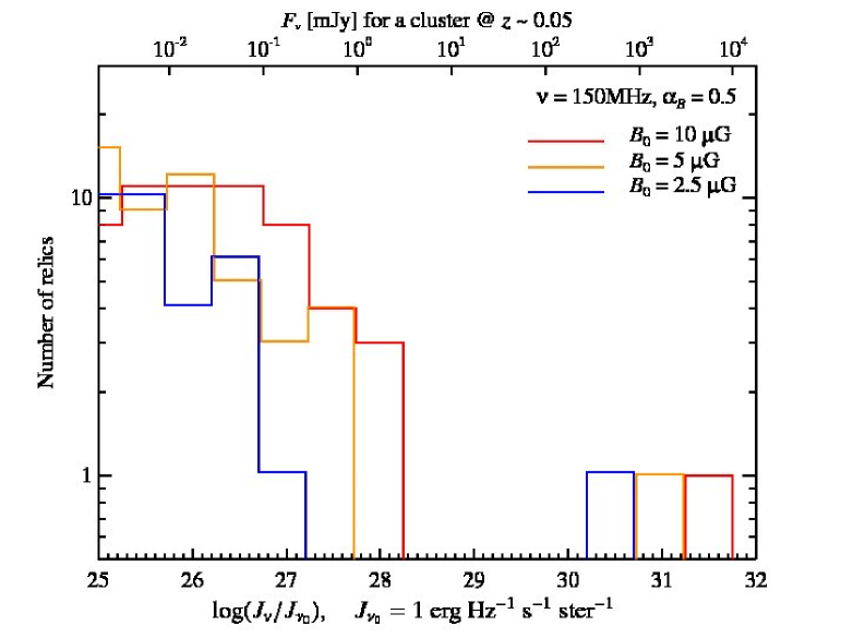
Figure 4: Luminosity functions with observable parameters (left) and theoretical parameters (right) of our relic finder. The top and bottom panels show how the magnetic decline $\alpha_{B}$ and the magnetic core energy density $B_{0}$ impact the luminosity functions, respectively. The choice of magnetic field parameters has a large impact on the shapes of the luminosity function which is a consequence of the inhomogeneous nature of virializing processes in cosmic structure formation. Smaller $\alpha_{B}$ values, corresponding to a shallower magnetic decline, produce many more brighter relics compared to larger values of $\alpha_{B}$, which produce slightly more less-luminous relics. Increasing $B_{0}$ results in a greater number of more-luminous relics. Notice the loss of the less-luminous relics from the observable to theoretical parameters. This is a result of the brightest relic swallowing up smaller relics due to a decrease of the emission threshold parameter.

2.4.2 Removal of galaxy contamination and cool core

Our radiative simulations model star formation (Hernquist & Springel, 2003) which leads to the formation of galaxies. When applying the criteria described in Sect. 2.4, these galaxies appear as false radio relic candidates since they are dense, compact and have enough emissivity per particle to be selected by the relic finder. To select against those objects, we impose further constraints on the SPH particles that are grouped together and require them to have a zero fraction of neutral hydrogen and to be below a very conservative threshold of number density $n_{\mathrm{thres}}=n_{\mathrm{SFT}}/32=0.004\mbox{ cm}^{-3}$.

Our relic finder also picks up the over-cooled centres of galaxy clusters in our simulations, contaminating the radio emission. Since the candidate relic in the over-cooled center may be physically connected to other true relics, it cannot be removed by simply discarding the closest relic candidate to the center. We apply a very conservative cut in radius of $r=40\mbox{ kpc}$ and neglect the weak dependence on cluster mass and dynamical state. We note that smaller clusters ($M<5\times 10^{14}\mathrm{M}_{\odot}$), in particular those with dynamical activity, tend to have slightly smaller cooling regions.

3 Results

3.1 Probing the intra cluster magnetic fields

In this section, we investigate how sensitive different radio synchrotron observables are with respect to the properties of the large scale magnetic field.

3.1.1 Luminosity functions

Rotation measure

Rotation angle

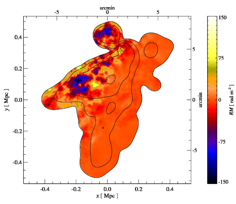
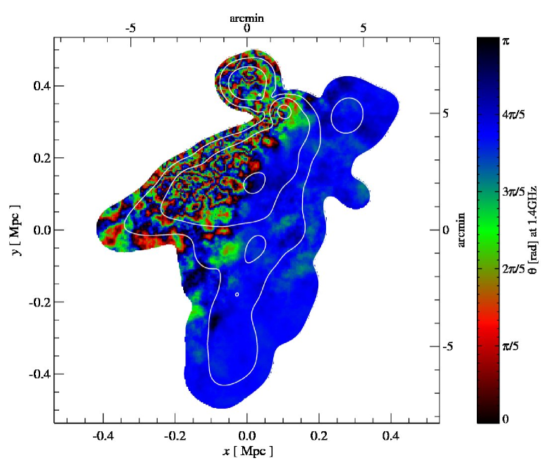
Figure 5: Left panel: Faraday rotation measure map of the largest relic in g72a, if the cluster were placed at z$\sim$0.05 (mimicking A2256). Right panel: Polarization angle map at $\nu=1.4$ GHz, assuming a uniform rotation angle at the position of the relic. The cluster center is located in the direction of the upper left corner for both the images. Regions with high RM variance correspond to high spatial variation of the polarization angle. In combination with a finite beam size, this makes it challenging to observe a high degree of polarization in such a relic. The magnetic field parameters are $\alpha_{B}$ = 0.7 $B_{0}$ = 2.5 $\mu$G and the contours represent the surface brightness increasing in decades from $5\times 10^{-3}$ mJy arcmin^-2 at $\nu$ = 1.4 GHz.

The magnetic fields within our simulations are parametrized by a simple scaling relation. For each cluster, we compute radio luminosity functions to aid in differentiating between different magnetic field parametrizations by employing the dependency of synchrotron emissivity on the magnetic field of the ICM. Our luminosity functions are distribution functions of the total luminosity per relic ($J_{\nu}$), where

$$J_{\nu}=\sum_{a}j_{\nu,a}\frac{M_{a}}{\rho_{a}}=\sum_{a}J_{\nu,a}.$$ (8)

The units of $J_{\nu,a}$ are erg s^-1 Hz^-1 ster^-1, $M_{a}$ and $\rho_{a}$ are the SPH gas particle mass and density respectively for the set of SPH particles within the relic labelled by $a$.

The number of relics seen depends on the magnetic field parametrization. In Fig. 4, we show how the luminosity functions depend on $B_{0}$ and $\alpha_{B}$. As expected, we find more and brighter radio relics for higher values of $B_{0}$. However, rather than simply scaling the luminosity function to higher relic emissivities for larger $B_{0}$ (assuming a fixed slope $\alpha_{B}$), we find that their shapes change. This is a consequence of the inhomogeneity of the virializing cosmic structure formation waves that are illuminated by the synchrotron emitting electrons. The effect of varying $B_{0}$ is analogous to the water level within a very inhomogeneous landscape that corresponds to the strength of the virializing shock waves. This level can adopt different values depending on the magnetic realization such that the resulting synchrotron emitting objects end up single connected or disjoint. So, one could consider using Minkowski functionals to characterize the different relics.

The trend for $\alpha_{B}$ is the opposite: higher values of $\alpha_{B}$ lead to a lower number of radio relics. The parameter $\alpha_{B}$ represents the slope of the magnetic scaling ($\varepsilon_{\mathrm{th}_{0}}>\varepsilon_{\mathrm{th}}$), and a steeper slope will result in the magnetic field strength falling off faster with radius. We expect the effect of both $B_{0}$ and $\alpha_{B}$ on the luminosity function to be a generic effect for all the simulated clusters, since $j_{\nu}\propto B^{\alpha_{\nu}+1}/(\varepsilon_{B}+\varepsilon_{\mathrm{CMB}})$ (cf. Eqns. 4 and 5) and in the peripheral cluster regions where $\varepsilon_{B}<\varepsilon_{\mathrm{CMB}}$, we obtain $j_{\nu}\propto B^{\alpha_{\nu}+1}$. The luminosity functions alone are not sufficient to fully disentangle the magnetic field properties, this will require other observables.

3.1.2 Rotation measure

Another independent approach to constrain magnetic field models are Faraday rotation measurements. Theoretically, one expects the magnetic field in shocks to be aligned with them due to shock compression (Enßlin et al., 1998) and stretching and shearing motions induced by oblique shocks (Schekochihin & Cowley, 2006). In combination with the small synchrotron emitting volume that is caused by the small synchrotron cooling time, this yields to polarized relic emission. Indeed, radio relics have been observed to be polarized up to the 40 per cent level (Feretti et al., 2004; Clarke & Enßlin, 2006). When polarized radio emission propagates through a magnetized medium, its plane of polarization rotates for a nonzero line-of-sight component of the magnetic field $B_{z}$ due to the birefringent property of the plasma – Faraday rotation. The Faraday rotation angle is given by

$$\Phi_{\mathrm{obs}}=\lambda^{2}RM+\Phi_{\mathrm{init}},$$ (9)

where

$$RM(\textbf{{x}}_{\bot}) = a_{0}\int_{0}^{L}B_{z}(\textbf{{x}})\,n_{\mathrm{e}}(\textbf{{x}})\,\mathrm{d}z$$ (10)

$$\simeq 812\,\frac{\mathrm{rad}}{\mathrm{m}^{2}}\,\frac{B}{\mu G}\,\frac{n_{\mathrm{e}}}{10^{-3}\mbox{ cm}}\,\frac{L}{\mbox{Mpc}},$$ (11)

where $a_{0}=e^{3}/(2\pi m_{\rm e}^{2}c^{4})$, $\textbf{{x}}=(\textbf{{x}}_{\bot},l)$, and $n_{\mathrm{e}}$ is the number density of electrons. In Eqn. 11, we have assumed constant values and a homogeneous magnetic field along the line-of-sight to give an order of magnitude estimate for RM values. Assuming statistically homogeneous and isotropic magnetic fields, the RM dispersion $\langle RM^{2}\rangle$ reads as follows,

$$\langle RM^{2}\rangle = a_{0}^{2}\left\langle\left[\int_{0}^{L}n_{\rm e}(\textbf{{x}})B_{z}(\textbf{{x}})\,\mathrm{d}z\right]^{2}\right\rangle$$ (12)

$$= a_{0}^{2}\frac{3\lambda_{B}}{2}L\,\langle n_{\rm e}(\textbf{{x}})^{2}B_{z}(\textbf{{x}})^{2}\rangle$$ (13)

$$= a_{0}^{2}\frac{3\lambda_{B}}{2}L\,\mathcal{C}_{n_{\mathrm{e}}B_{z}}\,\langle n_{\rm e}(\textbf{{x}})^{2}\rangle\langle B_{z}(\textbf{{x}})^{2}\rangle,$$ (14)

where

$$\mathcal{C}_{n_{\mathrm{e}}B_{z}}=\frac{\langle B_{z}^{2}n_{\mathrm{e}}^{2}\rangle}{\langle B_{z}^{2}\rangle\langle n_{\mathrm{e}}^{2}\rangle},$$ (15)

is defined as the correlation factor and $\lambda_{B}=2/3\times\lambda_{z}$ is the 3D magnetic auto-correlation scale (Enßlin & Vogt, 2003) which can be estimated from the measured $RM$ power spectrum.

We studied the Faraday rotation of the largest relic in cluster g72a (Fig. 5). The aim is to recover intrinsic statistical properties of the ICM magnetic field by studying RM statistics. We produce the RM map by projecting the line-of-sight component of our tangled magnetic field (Sect. 2.2) and the thermal electron density that has also been mapped from its Lagrangian distribution onto a 3D grid. Firstly, we are concerned about the observability of polarized emission. The RM scales with $B_{\parallel}$ and $n_{\rm e}$ according to Eqn. 10 such that we expect RM values to increase across the relic towards the projected cluster center. However, large RM values leads to confusion when trying to observe the polarization angle. Beam width depolarization (Gardner & Whiteoak, 1966) takes place if the polarization angle changes by a radian on scales shorter then the beam. To avoid this, one can go to shorter wavelengths and smaller beams at the expense of radio luminosity. Secondly, we are concerned with RM contamination from the galaxy. Even at moderately high galactic latitudes the galactic RM contribution (Simard-Normandin et al., 1981) can be approximately the same order as the RM we calculate. However, the strength of our RM depends on the relic location with respect to the cluster and observer, as well as our magnetic field parameters. Therefore, a different location or parametrization will lead to stronger or weaker RM. Also, the galactic RM in principle can be modelled and removed from the RM map.

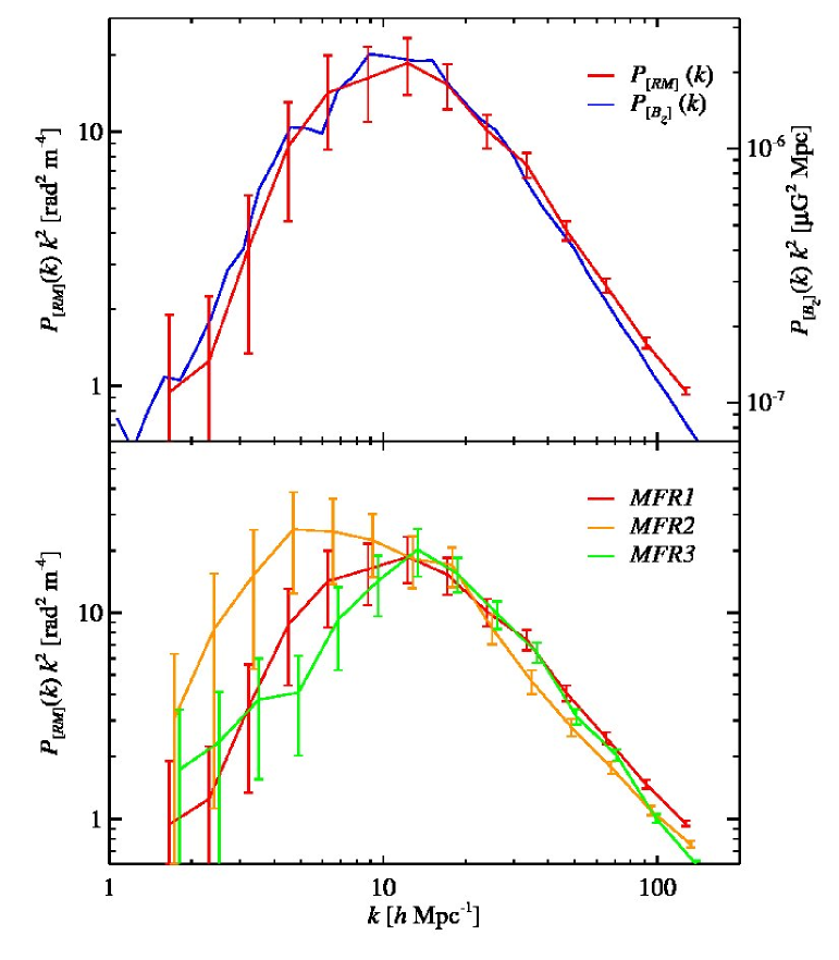
Figure 6: Top: power spectrum of the RM map $P_{[RM]}(k)$ and power spectrum of the line-of-sight component of the magnetic field $P_{[B_{z}]}(k)$ for MFR1, where the error bars represent the 1$\sigma$ confidence regions. $P_{[RM]}(k)$ attains excess power at large angular scales from fluctuations in $n_{\mathrm{e}}$. Our RM power spectrum matches the shape and the peak scale of the input power spectrum within the error bars. Bottom: power spectra of RM maps for different magnetic field realizations (cf. Table LABEL:tab:bfield). All RM power spectra recover the shape and characteristic scale of their magnetic input power spectra.

Table 4: Magnetic field realizations (MFR) used in RM maps.

magnetic field	correlation length	input slope of
realization name	($\lambda_{B}$) [$h^{-1}$ kpc]	power spectra
MFR1	100	-5/3
MFR2	200	-5/3
MFR3	100	-2

High-quality rotation measure maps enable one to measure the RM power spectra. The large angular extent of giant radio relics provides a powerful tool of probing the maximum coherence scales of the magnetic field in clusters; in contrast RM maps from radio lobes are typically much smaller. We calculate power spectra from our RM maps and magnetic field realizations for each model separately (Fig. 6 and Table LABEL:tab:bfield). For consistency reasons, we only consider the volume subtended by the radio relic when calculating the magnetic power spectrum. We define the RM power spectra ($P_{[RM]}$) and the power spectrum of $B_{z}$ ($P_{[B_{z}]}$) as follows,

$$\langle RM^{2}\rangle = 2\pi\int_{0}^{\infty}kP_{[RM]}\,\mathrm{d}k,$$ (16)

$$\langle B^{2}\rangle = 3\cdot 4\pi\int_{0}^{\infty}k^{2}P_{[B_{z}]}\,\mathrm{d}k,$$ (17)

where the additional factor of three accounts for fluctuations in the total magnetic field while assuming our random Gaussian field. A partial Monte Carlo method was used to determine the 1$\sigma$ error bars on the power spectrum. Assuming a constant magnetic coherence scale, we construct the envelope function by computing the variance of RM (Eqn. 13). We multiply this envelope function with $10^{3}$ realizations of random Gaussian field and measure the power spectrum on each of these maps. The fractional errors are computed from the variance of these power spectra. While the first six power spectrum bins are on average 50 per cent correlated, the correlations drop to be below 20 per cent for the bins on smaller scales.

By construction our parametrization of the magnetic field is correlated with the electron number density $n_{\mathrm{e}}$ which might possibly introduce biases in our RM maps. However, comparing RM power spectrum to the magnetic power spectrum, we find that the RM power spectrum overall resembles the original shape of the magnetic power spectrum and the injection scale corresponds to the scale of maximal power in the RM map. This is true for all our magnetic field realizations. We measure the slope of these power-laws at small scales to an accuracy of $\pm$0.05, which is significant to differentiate between Kolmogorov ($k^{-5/3}$) and Burgers ($k^{-2}$) turbulence spectra. We also find that the measurement of the RM power spectrum slope is independent of the magnetic field parameters $\alpha_{B}$ and $B_{0}$. The full correlation matrix of the power spectrum bins is used when fitting the power-laws and in the error calculations. We find that our measured slope is flatter then expected and can be attributed to small scale fluctuations in $n_{\mathrm{e}}$, since $P_{[B_{z}]}$ has the same slope as the power spectrum of $B_{z}$ integrated along the line of sight. The small inhomogeneity of $n_{\mathrm{e}}$ in our simulations does not severely affect the intrinsic spectral shape. Thus, it is possible in principle to recover the intrinsic 3D magnetic power spectrum by solving the inverse problem (Vogt & Enßlin, 2003; Enßlin & Vogt, 2003; Vogt & Enßlin, 2005).

Using Eqns. 14, 16 and 17 we estimated the rms magnetic field strength from $P_{[RM]}$ and $P_{[B_{z}]}$ respectively and recover our initial rms magnetic field strength. We find that our correlation factor ($\sqrt{C_{n_{\mathrm{e}}B_{z}}}\simeq 5.3$) is 20 per cent larger than the correlation factor obtained by fitting a smooth $\beta$-model to the spherically averaged profile of $n_{\mathrm{e}}$ and scaling $B\propto n_{\mathrm{e}}^{\alpha_{B}}$ with the same $\alpha_{B}=0.7$ that we used to construct our RM maps (similar to the procedure applied by Enßlin & Vogt 2003 and Murgia et al. 2004). This result suggests that the fairly homogeneous density distribution in our simulations (after removing the galaxy contamination described in Sect. 2.4.2) does not severely bias the average magnetic field strengths estimated by RM studies if one takes into account the overall shape of the profiles of $n_{\rm e}$ and $B$.

For convenience, we derive a formula for the rms magnetic field strength ($\sqrt{\langle B^{2}\rangle}$) as a function of the peak of $P_{[RM]}$ and the rms fluctuations of $n_{\rm e}$. Multiplying $P_{[RM]}$ with a Heaviside function $\Theta(k)$ and ensuring that the intrinsic spectrum is sufficiently steeper than $k^{-2}$, Eqn. 16 becomes

$$\langle RM^{2}\rangle \simeq 2\pi\int_{0}^{\infty}kP_{[RM]}(k)\,\Theta(k-k_{\mathrm{peak}})\,\mathrm{d}k,$$ (18)

$$\simeq \pi P_{[RM]}(k_{\mathrm{peak}})\,k_{\mathrm{peak}}^{2}.$$

The value of $P_{[RM]}(k_{\mathrm{peak}})\,k_{\mathrm{peak}}^{2}$ can be read off directly from Fig. 6 and combining Eqns. 18 and 14 yields an approximate value for $\sqrt{\langle B^{2}\rangle}$,

$$\sqrt{\langle B^{2}\rangle} \simeq \sqrt{\frac{{2\pi\,P_{[RM]}(k_{\mathrm{peak}})\,k_{\mathrm{peak}}^{2}}}{a_{0}^{2}\,\lambda_{B}\,L\,\mathcal{C}_{n_{\mathrm{e}}B_{z}}\,\langle n_{\rm e}^{2}\rangle}}$$

$$\simeq 0.1\mu\mathrm{G}\left(\frac{P_{[RM]}(k_{\mathrm{peak}})\,k_{\mathrm{peak}}^{2}}{50\,\mathrm{rad}\,\mathrm{m}^{-2}}\right)^{\frac{1}{2}}\left(\frac{\sqrt{\langle n_{\mathrm{e}}^{2}\rangle}}{10^{-4}\,h^{2}\,\mathrm{cm}^{-3}}\right)^{-1}$$

$$\times \left(\frac{\lambda_{B}}{100\,h^{-1}\,\mathrm{kpc}}\right)^{-\frac{1}{2}}\left(\frac{L}{4\,h^{-1}\,\mathrm{Mpc}}\right)^{-\frac{1}{2}}\left(\frac{\mathcal{C}_{n_{\mathrm{e}}B_{z}}}{27}\right)^{-\frac{1}{2}},$$ (20)

where we inserted numerical values from our simulation in the last step.

3.2 Existence and properties of the WHIM

In this section, we investigate the potential of radio relic observations to infer the hydrodynamic properties such as density and temperature of the WHIM.

3.2.1 Properties of virializing shocks

Spectral index projection of largest relic

Observed spectral index projection

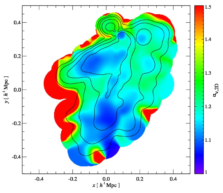
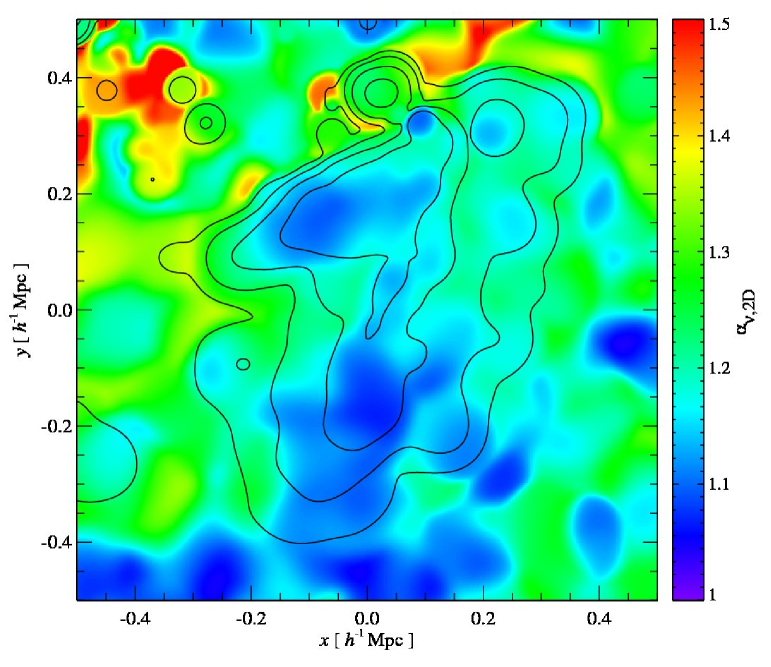
Figure 7: Spectral index map, $\alpha_{\nu,2D}$, between 150 MHz and 1.4 GHz for the largest relic in g72a, with only the SPH particles selected by the relic finder projected (left panel) and for the total emission in the same region (right panel). The contours show orders of magnitude in surface brightness in mJy arcmin^-2, with the highest contour representing 5 mJy arcmin^-2 at $\nu$ = 1.4 GHz. Notice the edge effects that show up in the projection of the single relic where the emission falls off. These effects are due to the sharp emissivity cutoff of our relic finder and incomplete sampling of SPH relic particles at different frequencies. More importantly, in regions with high synchrotron brightness, the spectral index is almost uniform across the central relic implying that this relic traces a single formation shock wave.

2D spectral index distributions

3D spectral index distributions

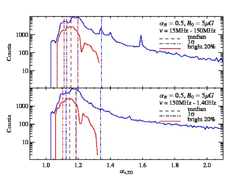
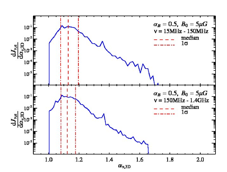
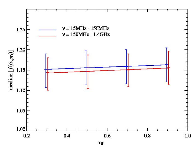
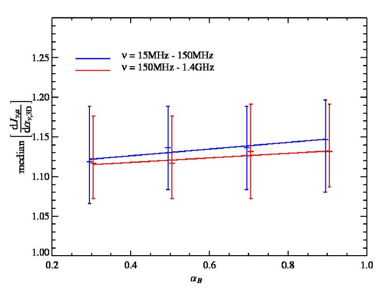
Figure 8: Top: spectral index distributions for our largest relic using our standard particular magnetic field parametrization. 2D spectral index distributions, $f(\alpha_{\nu\mathrm{2D}})$, of the full map and the brightest 20 percent pixels (top left) are contrasted to the radio luminosity weighted distribution of the 3D spectral index, $\mathrm{d}J_{\nu,a}/\mathrm{d}\alpha_{\nu,\mathrm{3D}}$ (top right). Bottom left: the median of $f(\alpha_{\nu\mathrm{2D}})$ for the brightest 20 percent pixels ($S_{\nu}\geq$ 12 mJy arcmin^-2 at $\nu$ = 150 MHz and $S_{\nu}\geq$ 1 mJy arcmin^-2 at $\nu$ = 1.4 GHz) as a function of the magnetic decline $\alpha_{B}$ with the error bars representing the 1$\sigma$ percentiles. Bottom right: the median of $\mathrm{d}J_{\nu,a}/\mathrm{d}\alpha_{\nu,\mathrm{3D}}$ as a function of the magnetic decline $\alpha_{B}$ with the error bars representing the 1$\sigma$ percentiles. This shows that for the giant radio relic of g72a, the median of the 2D and the 3D spectral indices agree statistically and are almost independent of the magnetic decline $\alpha_{B}$.

Diffusive shock acceleration determines the shape of the CRe spectrum that we model as a power-law momentum spectrum (neglecting non-linear effects). Synchrotron losses cause a steepening of this power-law by one power of momentum. Spatially inhomogeneous virializing shocks with a distribution of shock strengths cause a spatial variation of the spectral index of the cooled CR electron spectrum. This is reflected in an inhomogeneous distribution of synchrotron spectral index that may help to reconstruct the merging geometry by providing a snapshot of the structure formation process in a galaxy cluster.

The spectral indices of the radio surface brightness $\alpha_{\nu,\mathrm{2D}}$ and that of the intrinsic 3D emissivity $\alpha_{\nu,\mathrm{3D}}$ are defined by,

$$\alpha_{\nu,\mathrm{2D}}=-\frac{\log(\frac{S_{\nu}}{S_{\nu_{\mathrm{o}}}})}{\log(\frac{\nu}{\nu_{\mathrm{o}}})},$$ (21)

$$\alpha_{\nu,\mathrm{3D}}=-\frac{\log(\frac{J_{\nu,a}}{J_{\nu_{\mathrm{o}},a}})}{\log(\frac{\nu}{\nu_{\mathrm{o}}})}.$$ (22)

It is unclear ab initio whether the projected spectral index represents the actual deprojected quantity ($\alpha_{\nu,\mathrm{3D}}$) due to possible superposition of different radio emitting structures along the line-of-sight. We study how these two quantities relate to each other, and present 2D spectral index maps of both the largest radio relic in g72a and the total emission from the same area (cf. Fig. 7). We note that more than 99 per cent of the total radio emission can be attributed to emission within the radio relic. As a result, the $\alpha_{\nu,\mathrm{2D}}$ maps are not contaminated by the diffuse spurious emission. Note the edge effects in Fig. 7 that show up in the projection of the single relic where the emission falls off. These effects are due to the sharp emissivity cutoff of our relic finder and incomplete sampling of SPH relic particles at different frequencies. In regions with high synchrotron brightness, one can ignore these edge effects, and the resulting distribution of $\alpha_{\nu,\mathrm{2D}}$ is fairly uniform ($\langle\alpha_{\nu,\mathrm{2D}}\rangle\simeq$ 1.15, with $\sigma_{\alpha_{\nu,\mathrm{2D}}}\simeq$ 0.04) implying that this relic traces a single structure formation shock wave.

We further study the distribution of $\alpha_{\nu,\mathrm{2D}}$ and $\alpha_{\nu,\mathrm{3D}}$ in our largest individual relic to uncover a connection between them. Probability distribution functions (PDF) are constructed for both $\alpha_{\nu,\mathrm{2D}}$ and $\alpha_{\nu,\mathrm{3D}}$ for varying parameters of the magnetic field (cf. Fig. 8). To avoid contamination from edge effects seen in Fig. 7, the $\alpha_{\nu,\mathrm{2D}}$ PDF was made for the brightest 20 per cent of the pixels and the $\alpha_{\nu,\mathrm{3D}}$ PDF was weighted by particle emissivity. These distributions do not change with our choices for magnetic field parameters implying that the spectral indices are practically independent of the magnetic field and depends mainly on properties of the shock. Another striking result is that the median values for $\alpha_{\nu,\mathrm{2D}}$ and $\alpha_{\nu,\mathrm{3D}}$ are statistically consistent within 1-$\sigma$. Assuming that the line-of-sight integral is dominated by one bright relic and choosing a pixel scale that is smaller than the length scale on which the post-shock density varies, we can easily show that the 2D and intrinsic 3D spectral index are identical. If there are more radio emitting regions contributing to the observed surface brightness, we expect a concave radio spectrum. Synchrotron cooling as well as re-acceleration lead to spectral steepening in particular at high radio frequencies (Schlickeiser et al., 1987). Future work is required to address the associated biases of the relation between $\alpha_{\nu,\mathrm{2D}}$ and $\alpha_{\nu,\mathrm{3D}}$.

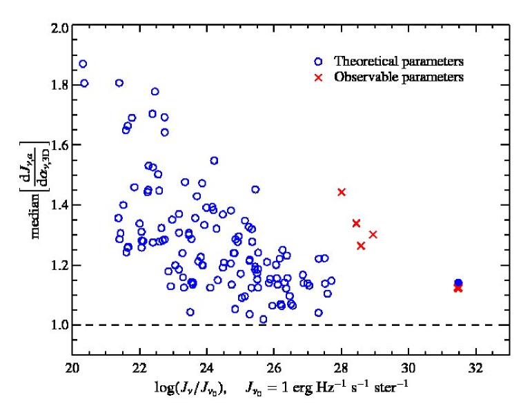
Figure 9: Two dimensional observable parameter space for radio relics in galaxy cluster g72a. Each symbol represents a relic within g72a and they are characterized by total luminosity and median of the 3D spectral index. Shown are observable relics (red crosses), theoretical relics (blue circles) and the large relic is emphasized by the bold cross and the filled circle. There is a trend to high spectral indices and a larger scatter for less luminous relics. As shown in Fig. 4, the loss of the less luminous relics from the observable to theoretical parameters is a result of the brightest relic swallowing up these smaller relics due to a decrease of the emission threshold parameter.

Figure 9 shows the observable parameters space of relic luminosity and the median 3D spectral index. This parameter space compares the shocks strength, which is related to the 3D spectral index (cf. Eqn. 27) to the energy dissipated at the shock, which is related to the relic luminosity. There is a trend that strong shocks are associated with the more luminous relics. The implications of this trend is that the brightest radio relics should show predominantly flatter spectral indices, which is the current observational status of giant radio relics (Ferrari et al., 2008).

3.2.2 Predicting pre-shock properties

A majority of the hot gas ($>10^{7}$ K) found at the centers of galaxy clusters is believed to originate from the WHIM that is shock heated through large-scale virializing structure formation shocks. These structure formation shocks are traced by synchrotron emission in form of radio relics from recently accelerated electrons (cf. Sect. 2.3). We have shown that under particular conditions, the observed median 2D spectral index corresponds to the weighted median 3D spectral index $\alpha_{\nu,\mathrm{3D}}$ (cf. Sect. 3.2.1). The 3D spectral index can be related to the Mach number of the shock (cf. Eqn. 27) under the assumption that we have an ideal fluid with a given adiabatic index. One can obtain information on the post-shock values for density, pressure and temperature of the ICM through deprojections of deep X-ray or Sunyaev-Zel’dovich observations (Zaroubi et al., 1998). With the knowledge of the Mach numbers combined with post-shock values we calculate the pre-shock conditions of the ICM (the WHIM) using the Rankine-Hugoniot jump conditions (cf. Appendix C).

We take an optimistic approach and assume that the deprojections of the thermal observables can be done ideally such that we use our radial profiles calculated from the solid angle subtended by the largest relic for simplicity (cf. Fig. 10). We define the shock region by locating the radial bins that contain the majority of shocked relic particles ($>85\%$). A small fraction of the relic particles leak into radial bins adjacent to the shock causing slight enhanced values of the radial profile. As mentioned above we insert the calculated average Mach number and the post-shock value into the Rankine-Hugoniot jump conditions for density, pressure and temperature to estimate the upper limits of these WHIM properties. Our predicted upper limits for pressure and temperature of the WHIM are consistent with the simulated pre-shock properties within one standard deviation. We note that the standard deviation of these hydrodynamic properties reflect actual physical variations due to an oblique shock that is not perfect tangential. Additionally, the particular relic chosen is located at $\sim R_{200}/2$, which is within the cluster volume. There are other observationally know relics that reside at the virial radius and beyond (e.g. Bagchi et al., 2006). These relic are better suited to probe the WHIM in combination with future X-ray and multi-frequency SZ data. Thus, this example is to be taken as a demonstration of our concept.

In the following we want to address possible biases with our method and show that the discrepancy between the predicted values and the average radial value of the WHIM can be explained by differences between the calculated Mach numbers and the median of the weighted Mach numbers in the radio relics (cf. Fig. 11). We find that the weighted Mach numbers have systematically lower values compared to the theoretical expectation due to the skewed distribution of the emissivity weighted $\alpha_{\nu,\mathrm{3D}}$. According to the Rankine-Hugoniot jump conditions, systematically higher values of the shock strength should over-estimate the jumps and hence under-predict all the pre-shock quantities, which appears to be the case (Fig. 10).

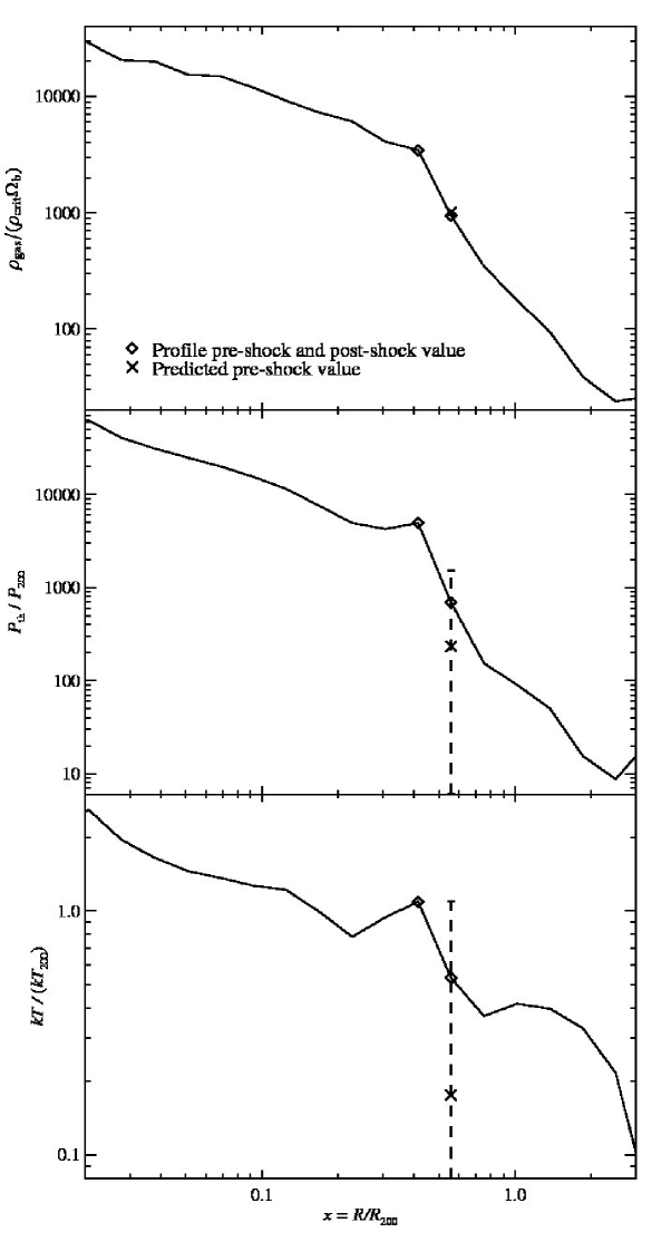
Figure 10: Radial profiles of galaxy cluster g72a restricted to the solid angle subtended by the largest relic for the density, pressure and temperature. The shocked region is seen in the profile at roughly $R_{200}/2$ and is marked by the black diamonds with one sigma error bars, except for the density profile where the error bars are too small to show. The predicted pre-shock values (crosses) are $\sim$ 7%, $\sim$ 67% and $\sim$ 67% different from the average profile values, but fall within the standard deviation for pressure and temperature. Most of this variation is caused by the shock being oblique and not perfectly tangential.

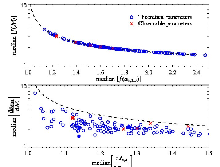
Figure 11: Top: median of the Mach number distribution for each relic as a function of the median of the distribution function of $\alpha_{\nu,\mathrm{3D}}$. Bottom: the observationally relevant quantities are the weighted distribution functions. Shown are median of $\mathrm{d}\dot{\varepsilon}_{\mathrm{diss}}/\mathrm{d}\mathcal{M}$ as a function of $\mathrm{d}J_{\nu,a}/\mathrm{d}\alpha_{\nu,\mathrm{3D}}$, where each point represents a radio relic in cluster g72a. Shown are observable relics (red crosses), theoretical relics (blue circles) and the large relic is emphasized by the bold cross and the filled circle. The dashed line is the theoretical Mach number computed from directly from the $\alpha_{\nu,\mathrm{3D}}$ (cf. Appendix Eqn. 27). The theoretical Mach number over-predicts the median of the weighted Mach number, due to the weighting of $\alpha_{\nu,\mathrm{3D}}$ by the skewed distribution function of the radio luminosity.

3.3 Dependence on dynamical state and cluster mass

Observable parameters

Theoretical parameters

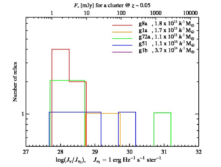
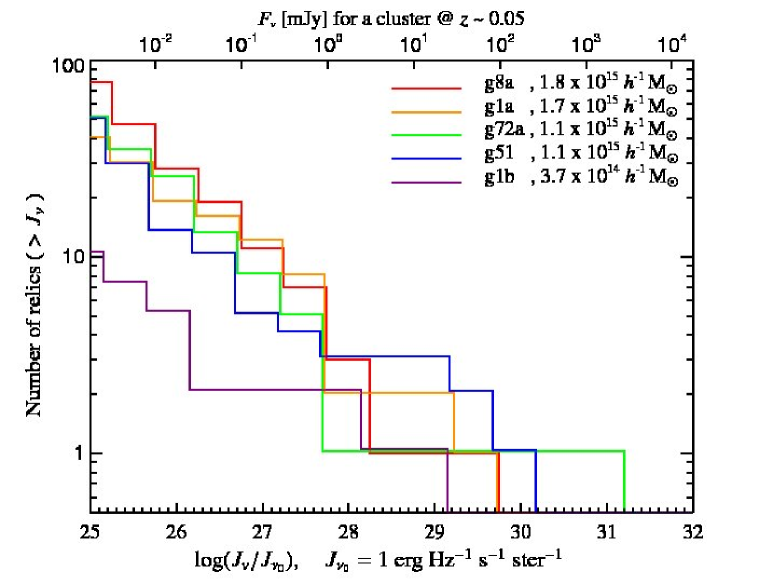
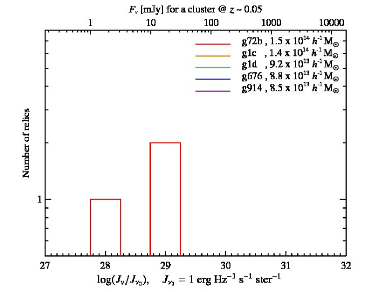
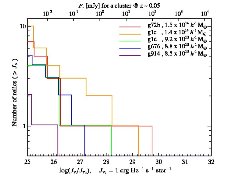
Figure 12: Luminosity functions for our sample of 10 clusters with the high mass clusters ($M_{\mathrm{vir}}>2\times 10^{14}\,h^{-1}\mathrm{M}_{\sun}$) in the upper panels and the low mass clusters in the lower panels for our standard magnetic model at 150 MHz (see Table LABEL:tab:bpar). The left panels contain relics found using the observable parameters and the right panels contain the theoretical parameters. The luminosity functions from the observable parameters show that more massive clusters have relics while low mass clusters have no relics (with g1b and g72b being the exceptions in both cases, respectively). The cumulative luminosity functions from the theoretical parameters show the trend for higher mass clusters to contain more relics and dynamical cluster stage modulates this effect notably, especially at low cluster masses. For instance compare the luminosity functions of the equal mass clusters g51 and g72a, the latter of which is a post-merging cluster.

We study the distribution of radio relics for the entire galaxy cluster sample, which shows a variety of both dynamical states (ranging from merging to cool core clusters) and masses (a range of almost two orders of magnitude). In Fig. 12, we investigate how cluster mass and dynamical state depend on the relic luminosity function. In the case of our theoretical parameter space, more massive galaxy clusters clearly have more radio relics than the lower mass clusters with a power-law scaling of $M_{200}^{0.9}$ (Fig. 13). For the current observational capabilities, we predict that only the most massive clusters should have a significant sample of radio relics.

Ideally, one would like to directly compare clusters with the purpose of using relic number statistics as a mass proxy. However, the luminosity functions have another trend, which causes the scatter in the relationship between clusters mass and total number of relics per cluster. This trend relates the cluster’s dynamical state to the luminosity of their brighter relics. The clusters g72a and g51 have the same virial mass $1.1\times 10^{15}$ M_☉, but g51 is a relaxed cool core clusters in contrast to the active state of g72a. One can see the two most luminous radio relics of g72a are an order of magnitude brighter than any of g51’s relics. Furthermore, the total amount of relics of g72a is greater than that of g51. Merging clusters inherently have more shocks which yields to more high-energy CRes and magnetic field amplification resulting in more radio relics. This trend is even more severe for galaxy clusters of smaller mass (Fig 12). Our results show a larger probability of observing a relic in a more massive cluster that is dynamically active. This dependence on mass and dynamical state offers a possible explanation for why all current observed radio relics are in massive merging clusters. They are expected to be the brightest of a dimmer population of radio relics.

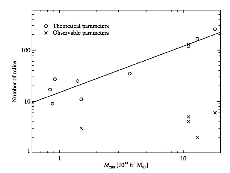
Figure 13: Relation between the number of radio relics within a galaxy cluster and the cluster mass, where each point represents one of our simulated clusters and the line represent the best fit power-law that scales as $M_{200}^{0.9}$. There is a trend for higher mass clusters to contain more relics.

4 Discussion

4.1 Comparison with previous theoretical work

Previously, there has been analytical work (Keshet et al., 2004a) and pioneering cosmological simulations (Miniati et al., 2001; Miniati et al., 2000) on studying cluster synchrotron emission from shock-accelerated electrons. The latter authors simulated the non-thermal cluster emission by numerically modelling discretised cosmic ray (CR) energy spectra on top of Eulerian grid-based cosmological simulations. Their approach neglected the hydrodynamic pressure of the CR proton component, was quite limited in its adaptive resolution capability, and neglected dissipative gas physics including radiative cooling, star formation, and supernova feedback. To allow studies of the dynamical effects of CR protons in radiatively cooling galactic and cluster environments, a CR proton formalism was developed that is based on smoothed particle hydrodynamical representation of the equations of motion (Pfrommer et al., 2006; Enßlin et al., 2007; Jubelgas et al., 2008). The emphasis is given to the dynamical impact of CR protons on hydrodynamics, while simultaneously allowing for the important CR proton injection and loss processes in a cosmological setting. Pfrommer et al. (2008) modelled the CR electron components due to shock acceleration as well as those being produced in hadronic CR proton interaction with ambient gas protons. Using this formalism and modelling, Pfrommer et al. (2007, 2008) and Pfrommer (2008) coherently studied the non-thermal cluster emission, the cosmic ray pressure component, and its implications for thermal cluster observables such as the X-ray emission and the Sunyaev-Zel’dovich effect. The focus of Miniati et al. (2001) was on primary CRe synchrotron emission from galaxy clusters as a whole, whereas we focused in this work on the emission from individual relics in detail to study the synchrotron observables and how they are sensitive to the large scale magnetic properties. To summarize, we have improved on past work in the observable predictions, simulations and observational understanding of non-thermal emission from primary accelerated CRe.

Additionally, we point out that IC and $\gamma$-ray emission are alternate ways to study structure formation shocks. This was proposed in analytical work by Loeb & Waxman (2000) and in simulations (Miniati, 2003; Keshet et al., 2003; Miniati et al., 2007; Pfrommer et al., 2008; Pfrommer, 2008). We are optimistic that high energy $\gamma$-ray experiments, such as the Fermi $\gamma$-ray space telescope (formely GLAST) and future imaging air Čerenkov telescopes, will aid in further developing the picture of non-thermal emission at structure formation shocks.

4.2 Assumptions

In our attempt to model diffuse radio relic emission from galaxy clusters, we have made several simplifying assumptions. (1) We assume the modified thermal leakage model fully describes the process of diffusive shock acceleration and did not vary the parameters associated with it. The described observations allow one to test the self-consistency of this hypothesis, and might finally allow improvement of our knowledge about diffusive shock acceleration in high-$\beta$ plasmas. (2) We neglect at this point the modifications of this simple model due to non-linear shock acceleration, as well as cosmic ray modified shocks, and postpone their study until future work. (3) We also neglect re-acceleration of mildly relativistic electrons that have been injected in the past either by formation shocks or other sources such as AGN. (4) We use a simple parametrization for the magnetic field. There are indications that the main characteristics of this model are realized in clusters on average (Vogt & Enßlin, 2005; Murgia et al., 2004). Future work has to be dedicated to study the distribution of magnetic fields that follow the magneto-hydrodynamics in radiative simulations. (5) We are solving for a steady-state spectrum of the electron population and are not sensitive to spectral aging processes across the relic as they may have been found recently by Giacintucci et al. (2008). (6) In our model, we assume the thermal reservoir to be the source of electrons. (7) In our analysis, we only consider the rotation measure signal from the line-of-sight integration of the density weighted parallel magnetic field. We explicitly neglect possible contributions from magnetic field amplifications due to post-shock turbulence local to the shock wave (Vladimirov et al., 2006; Ryu et al., 2008). These questions are beyond the scope of this work and will be studied elsewhere. (8) The mass contained within the relics is not a physically relevant quantity and suffers from the finite resolution of the SPH technique at the dilute shocks in the virial regions of clusters and beyond. The radio luminosity, however, is a robust prediction within a given acceleration model since it reflects conserved quantities such as energy and mass across the shock.

5 Conclusions

The intermittency and inhomogeneous nature of structure formation shocks are characterized by a highly non-Gaussian distribution function. This requires numerical simulations to study the implied non-universality of the induced radio relic (or gischt) emission. It is hard to conceive of an adequate analytical approach to this problem. Observing the polarized emission of a sample of relics at different frequencies enables us to gain insight into the non-equilibrium processes at work – in particular into the interplay of large scale magnetic fields and structure formation shocks. The relevant observables of the relics include morphology, spectral shape, relic luminosity function and Faraday rotation measure. The theoretical implications of radio relic observables are as follows:

We model the shock acceleration of electrons at formation shocks and find that the morphology of radio relics unambiguously characterises the underlying structure of dissipating shock waves (Fig. 1). The resulting simulated relics are very similar to the observed relics and thus support our hypothesis. Their positions identify regions that are not in equilibrium and where the electron and ion temperatures are expected to show strong deviations due to the comparatively long Coulomb mean free path that governs their equilibration process.

The relic luminosity function is sensitive to the combination of normalization and scaling properties of the magnetic field with thermal energy density as well as the electron acceleration efficiency, the mass and dynamical state of a cluster. Thus, it can provide hints about the processes that generate these large scale fields and can help to disentangle the dominant transport processes which include effects from magnetic flux freezing and growth by turbulent dynamos.

The rotation measure (RM) map is sensitive to the line-of-sight integrated magnetic field. From the mean and variance of RM maps, we can infer the location of the formation shock with respect to the cluster center as the variance increases as a function of integration length (Eqn. 14). This helps in constraining the geometry of the merger. Deprojecting the 2D RM power spectrum enables one to measure the 3D magnetic power spectrum, under the assumption that the behaviour of the electron density along the line of sight can be obtained from X-ray measurements. The peak of the 3D power spectrum yields the total magnetic energy and the magnetic coherence length $\lambda_{B}$. Performing this procedure for different relics or for different regions of one large relic allows us to estimate the variance of $\lambda_{B}$ across the cluster and might possibly tell us about the nature of MHD turbulence. We found that the correlation between $n_{\rm e}$ and $B$ biases the rms magnetic field strength derived from RM maps high if this is not taken into account; we note that most works have done so. This correlation should be a natural consequence of MHD effects such as flux freezing. If systematic errors associated with RM studies are smaller than statistical ones, we find that measurements of the small scale slope of the RM power spectrum are accurate enough to differentiate between Kolmogorov ($k^{-5/3}$) and Burgers ($k^{-2}$) turbulence spectra. The interpretation of these slopes is however not straight forward and needs to account for an additional flattening due to small scale fluctuations in $n_{\mathrm{e}}$.

The spectral index of a power law spectrum of a radio relic is a measure of the shock strength of that relic. The median spectral index of a distribution of relics probes a distribution of virializing shocks and can give an indication of CR proton injection. This is of particular relevance for questions concerning the pressure contribution of non-thermal components and enables comparison with predictions of hydrodynamical simulations. The shape of the spectrum is sensitive to the acceleration mechanism of the relativistic electrons and to their cooling processes. The variation of the spectrum over the relic allows one to infer in situ magnetic field strengths by comparing the synchrotron and IC cooling times to the advection time downstream provided that the magnetic energy density is not much smaller than the CMB energy density. This might constrain models for the magnetic amplification at shocks in high beta plasmas. A radio relic’s luminosity is roughly correlated with the shock strength. Thus, it is favourable to look for radio relics in large, dynamically disturbed clusters, or use relic detections as a proxy for dynamical activity of clusters (Schuecker et al., 2001).

We demonstrated that the combination of the relic spectral index with deprojected X-ray and SZ profiles allows one to indirectly infer upper limits on the density and temperature of the warm hot intergalactic medium. Simulations show that the WHIM is not uniform, rather it is characterized by highly inhomogeneous structure that shows intermittent accretion events that are channeled mostly through filaments.

We predict that there will be a large sample of polarized radio relics from a considerable number clusters in the near future. This sample should allow one to constrain macroscopic model parameters, which are expected to be higly non-Gaussian, using a joint analysis method on the radio observables. For example, the combination of the relic luminosity function, RM power spectra, X-ray and SZ measurements should constrain the models of diffusive shock acceleration and large scale magnetic fields. Future work will address the details of this procedure.

Appendix A Interpolating and projecting SPH quantities

In the course of this work we are required to interpolate our Lagrangian energy density distribution as given by SPH on a 3D grid. We remind the reader that the SPH smoothing kernel of an SPH particle $a$, $W(|\textbf{{r}}-\textbf{{r}}_{a}|,h_{a})$, is given by Eqn. A.1 of Springel et al. (2001). It is normalized in the continuum such that $\int W(r,h)\mathrm{d}^{3}\textbf{{r}}\equiv 1$. A scalar field $x(\textbf{{r}})$ is interpolated onto a 3D grid cell at $\textbf{{r}}_{ijk}$ by the product of itself with the specific volume $M_{a}/\rho_{a}$ of the gas particles over a comoving cube,

$$x(\textbf{{r}}_{ijk})=\frac{1}{L^{3}_{\mathrm{pix}}}\sum_{a}x_{a}\frac{M_{a}}{\rho_{a}}{\mathcal{W}}_{a,ijk}(|\textbf{{r}}_{ijk}-\textbf{{r}}_{a}|,h_{a}),$$ (23)

where $L^{3}_{\mathrm{pix}}$ is the comoving volume of the grid cell and we define the normalized 3D smoothing kernel of SPH particle $a$ at the grid position $\textbf{{r}}_{ijk}$ by

$${\mathcal{W}}(|\textbf{{r}}_{ijk}-\textbf{{r}}_{a}|,h_{a})=\frac{W(|\textbf{{r}}_{ijk}-\textbf{{r}}_{a}|,h_{a})}{\sum_{ijk}W(|\textbf{{r}}_{ijk}-\textbf{{r}}_{a}|,h_{a})}.$$ (24)

We note that the normalized interpolation conserves the interpolated quantity strictly without any further requirement on the grid size.

Similarly, we employ the method of normalized projection of a three dimensional SPH scalar fields $x(\textbf{{r}})$ to perform projection integrals yielding the quantity $X(\textbf{{r}}_{\perp})$. In analogy to Eqn. 23 we obtain

$$X(\textbf{{r}}_{\perp,ij})=\frac{1}{L^{2}_{\mathrm{pix}}}\sum_{a}x_{a}\frac{M_{a}}{\rho_{a}}\mathcal{Y}_{a,ij}(|\textbf{{r}}_{\perp,ij}-\textbf{{r}}_{a}|,h_{a}),$$ (25)

where $L^{2}_{\mathrm{pix}}$ is the comoving area of the pixel and the normalized 2D projected smoothing kernel of SPH particle $a$ at the grid position $\textbf{{r}}_{\perp,ij}$ derives from the projected SPH kernel $Y(|\textbf{{r}}_{\perp,ij}|,h_{a})$ and is given by

$$\mathcal{Y}(|\textbf{{r}}_{\perp,ij}-\textbf{{r}}_{a}|,h_{a})=\frac{Y(|\textbf{{r}}_{\perp,ij}-\textbf{{r}}_{a}|,h_{a})}{\sum_{ijk}Y(|\textbf{{r}}_{\perp,ij}-\textbf{{r}}_{a}|,h_{a})}.$$ (26)

Appendix B Theoretical emission threshold

The emission threshold for the observable parameters and theoretical parameters differ by 12 orders of magnitude. This dynamic range is beyond the ability of any future telescope on the horizon. Varying the emission threshold of our theoretical parameters by six orders of magnitudes only very weakly affects our results. In particular, we show in Fig. 14 that such a dramatic variation has only little influence on the high-end of the radio relic luminosity function.

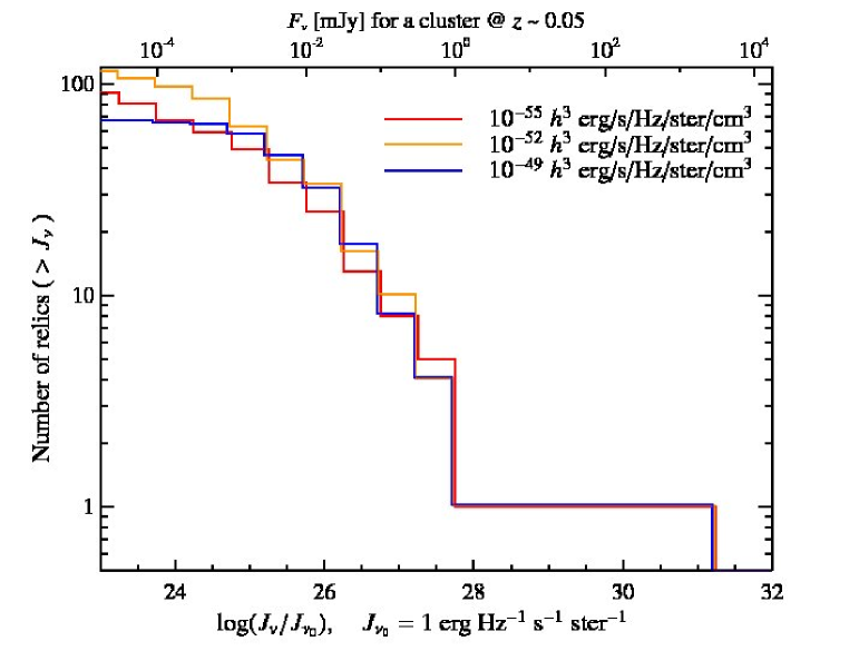
Figure 14: Cumulative luminosity functions for different values of the emission cutoff. This shows the robustness of our predictions for future instrument capabilities.

Appendix C Rankine-Hugoniot conditions

The three dimensional spectral index can be transformed into a Mach number ($\mathcal{M}$) (Enßlin et al., 2007), if one assumes an ideal fluid that is characterized a a single adiabatic index $\gamma$,

$$\mathcal{M}=\sqrt{\frac{4(1+\alpha_{\nu,\mathrm{3D}})}{1+4\alpha_{\nu,\mathrm{3D}}-3\gamma}}.$$ (27)

Under these conditions, the well-known Rankine-Hugoniot jump conditions allow to relate the hydrodynamic post-shock quantities (denoted with a subscript 2) to the pre-shock quantities (denoted with a subscript 1),

$$\frac{\rho_{1}}{\rho_{2}} = \frac{(\gamma-1)\mathcal{M}^{2}+2}{(\gamma+1)\mathcal{M}^{2}},$$ (28)

$$\frac{T_{1}}{T_{2}} = \frac{(\gamma+1)^{2}\mathcal{M}^{2}+2}{\left[2\gamma\mathcal{M}^{2}-(\gamma-1)\right]\left[(\gamma-1)\mathcal{M}^{2}+2\right]},$$ (29)

$$\frac{P_{1}}{P_{2}} = \frac{\gamma+1}{2\gamma\mathcal{M}^{2}-(\gamma-1)}.$$ (30)

Phenomenologically, we show in Fig. 11 that Eqn. 27 under-predicts the average $\langle\mathcal{M}\rangle$ if one were to infer $\mathcal{M}$ from spectral index maps. This translates into an upper limit for the predicted pre-shock density. In the case of temperature and pressure, the under-prediction of the average $\langle\mathcal{M}\rangle$ leads to an over-estimation of the pre-shock values which translates into lower limits for temperature and pressure (Eqns. 29 and 30).

References

- Ananthakrishnan (1995) Ananthakrishnan S., 1995, Journal of Astrophysics and Astronomy Supplement, 16, 427
- Bagchi et al. (2006) Bagchi J., Durret F., Neto G. B. L., Paul S., 2006, Science, 314, 791
- Balsara (1998) Balsara D. S., 1998, ApJS, 116, 133
- Beck (2001) Beck R., 2001, Space Science Reviews, 99, 243
- Beck et al. (1996) Beck R., Brandenburg A., Moss D., Shukurov A., Sokoloff D., 1996, ARA&A, 34, 155
- Blandford & Eichler (1987) Blandford R., Eichler D., 1987, Phys. Rept., 154, 1
- Bridle & Fomalont (1976) Bridle A. H., Fomalont E. B., 1976, A&A, 52, 107
- Bridle et al. (1979) Bridle A. H., Fomalont E. B., Miley G. K., Valentijn E. A., 1979, A&A, 80, 201
- Carilli & Taylor (2002) Carilli C. L., Taylor G. B., 2002, ARA&A, 40, 319
- Cavaliere & Fusco-Femiano (1978) Cavaliere A., Fusco-Femiano R., 1978, A&A, 70, 677
- Cen & Ostriker (1999) Cen R., Ostriker J. P., 1999, ApJ, 514, 1
- Clarke & Enßlin (2006) Clarke T. E., Enßlin T., 2006, Astronomische Nachrichten, 327, 553
- Danforth & Shull (2005) Danforth C. W., Shull J. M., 2005, ApJ, 624, 555
- Davé et al. (2001) Davé R., Cen R., Ostriker J. P., Bryan G. L., Hernquist L., Katz N., Weinberg D. H., Norman M. L., O’Shea B., 2001, ApJ, 552, 473
- Dolag et al. (1999) Dolag K., Bartelmann M., Lesch H., 1999, A&A, 348, 351
- Dolag et al. (2005) Dolag K., Grasso D., Springel V., Tkachev I., 2005, Journal of Cosmology and Astro-Particle Physics, 1, 9
- Drury (1983) Drury L. O., 1983, Reports of Progress in Physics, 46, 973
- Dubois & Teyssier (2008) Dubois Y., Teyssier R., 2008, A&A, 482, L13
- Ellison et al. (1981) Ellison D. C., Jones F. C., Eichler D., 1981, Journal of Geophysics Zeitschrift Geophysik, 50, 110
- Enßlin et al. (1998) Enßlin T. A., Biermann P. L., Klein U., Kohle S., 1998, A&A, 332, 395
- Enßlin & Gopal-Krishna (2001) Enßlin T. A., Gopal-Krishna 2001, A&A, 366, 26
- Enßlin et al. (2007) Enßlin T. A., Pfrommer C., Springel V., Jubelgas M., 2007, A&A, 473, 41
- Enßlin & Vogt (2003) Enßlin T. A., Vogt C., 2003, A&A, 401, 835
- Feretti et al. (2004) Feretti L., Burigana C., Enßlin T. A., 2004, New Astronomy Review, 48, 1137
- Ferrari et al. (2008) Ferrari C., Govoni F., Schindler S., Bykov A. M., Rephaeli Y., 2008, Space Science Reviews, 134, 93
- Fukugita (2004) Fukugita M., 2004, in Ryder S., Pisano D., Walker M., Freeman K., eds, Dark Matter in Galaxies Vol. 220 of IAU Symposium, Cosmic Matter Distribution: Cosmic Baryon Budget Revisited. p. 227
- Furlanetto & Loeb (2004) Furlanetto S. R., Loeb A., 2004, ApJ, 611, 642
- Gardner & Whiteoak (1966) Gardner F. F., Whiteoak J. B., 1966, ARA&A, 4, 245
- Geller & Huchra (1983) Geller M. J., Huchra J. P., 1983, ApJS, 52, 61
- Giacintucci et al. (2008) Giacintucci S., Venturi T., Macario G., Dallacasa D., Brunetti G., Markevitch M., Cassano R., Bardelli S., Athreya R., 2008, A&A, 486, 347
- Govoni et al. (2006) Govoni F., Murgia M., Feretti L., Giovannini G., Dolag K., Taylor G. B., 2006, A&A, 460, 425
- Grasso & Rubinstein (2001) Grasso D., Rubinstein H. R., 2001, Phys. Rept., 348, 163
- Guidetti et al. (2008) Guidetti D., Murgia M., Govoni F., Parma P., Gregorini L., de Ruiter H. R., Cameron R. A., Fanti R., 2008, A&A, 483, 699
- Haardt & Madau (1996) Haardt F., Madau P., 1996, ApJ, 461, 20
- Hellsten et al. (1998) Hellsten U., Gnedin N. Y., Miralda-Escudé J., 1998, ApJ, 509, 56
- Hernquist & Springel (2003) Hernquist L., Springel V., 2003, MNRAS, 341, 1253
- Jubelgas et al. (2008) Jubelgas M., Springel V., Enßlin T., Pfrommer C., 2008, A&A, 481, 33
- Kang et al. (2005) Kang H., Ryu D., Cen R., Song D., 2005, ApJ, 620, 21
- Kassim et al. (2005) Kassim N. E., Polisensky E. J., Clarke T. E., Hicks B. C., Crane P. C., Stewart K. P., Ray P. S., Weiler K. W., Rickard L. J., Lazio T. J. W., Lane W. M., Cohen A. S., Nord M. E., Erickson W. C., Perley R. A., 2005, in Kassim N., Perez M., Junor W., Henning P., eds, Astronomical Society of the Pacific Conference Series Vol. 345 of Astronomical Society of the Pacific Conference Series, The Long Wavelength Array. p. 392
- Katz et al. (1996) Katz N., Weinberg D. H., Hernquist L., 1996, ApJS, 105, 19
- Katz & White (1993) Katz N., White S. D. M., 1993, ApJ, 412, 455
- Kempner et al. (2004) Kempner J. C., Blanton E. L., Clarke T. E., Enßlin T. A., Johnston-Hollitt M., Rudnick L., 2004, in Reiprich T., Kempner J., Soker N., eds, The Riddle of Cooling Flows in Galaxies and Clusters of galaxies Conference Note: A Taxonomy of Extended Radio Sources in Clusters of Galaxies. p. 335
- Keshet et al. (2004a) Keshet U., Waxman E., Loeb A., 2004a, ApJ, 617, 281
- Keshet et al. (2004b) Keshet U., Waxman E., Loeb A., 2004b, New Astronomy Review, 48, 1119
- Keshet et al. (2003) Keshet U., Waxman E., Loeb A., Springel V., Hernquist L., 2003, ApJ, 585, 128
- Komatsu et al. (2008) Komatsu E., Dunkley J., Nolta M. R., Bennett C. L., Gold B., Hinshaw G., Jarosik N., Larson D., Limon M., Page L., Spergel D. N., Halpern M., Hill R. S., Kogut A., Meyer S. S., Tucker G. S., Weiland J. L., Wollack E., Wright E. L., 2008, ApJS submitted, arXiv:0803.0547
- Kronberg (1994) Kronberg P. P., 1994, Reports of Progress in Physics, 57, 325
- Kulsrud (1999) Kulsrud R. M., 1999, ARA&A, 37, 37
- Loeb & Waxman (2000) Loeb A., Waxman E., 2000, Nature, 405, 156
- Malkov & O’C Drury (2001) Malkov M. A., O’C Drury L., 2001, Reports of Progress in Physics, 64, 429
- Masson & Mayer (1978) Masson C. R., Mayer C. J., 1978, MNRAS, 185, 607
- Miniati (2003) Miniati F., 2003, MNRAS, 342, 1009
- Miniati et al. (2001) Miniati F., Jones T. W., Kang H., Ryu D., 2001, ApJ, 562, 233
- Miniati et al. (2007) Miniati F., Koushiappas S. M., Di Matteo T., 2007, ApJL, 667, L1
- Miniati et al. (2000) Miniati F., Ryu D., Kang H., Jones T. W., Cen R., Ostriker J. P., 2000, ApJ, 542, 608
- Morales et al. (2006) Morales M. F., Bowman J. D., Cappallo R., Hewitt J. N., Lonsdale C. J., 2006, New Astronomy Review, 50, 173
- Murgia et al. (2004) Murgia M., Govoni F., Feretti L., Giovannini G., Dallacasa D., Fanti R., Taylor G. B., Dolag K., 2004, A&A, 424, 429
- Pfrommer (2008) Pfrommer C., 2008, MNRAS, 385, 1242
- Pfrommer et al. (2008) Pfrommer C., Enßlin T. A., Springel V., 2008, MNRAS, 385, 1211
- Pfrommer et al. (2007) Pfrommer C., Enßlin T. A., Springel V., Jubelgas M., Dolag K., 2007, MNRAS, 378, 385
- Pfrommer et al. (2006) Pfrommer C., Springel V., Enßlin T. A., Jubelgas M., 2006, MNRAS, 367, 113
- Pizzo et al. (2008) Pizzo R. F., de Bruyn A. G., Feretti L., Govoni F., 2008, A&A, 481, L91
- Price & Monaghan (2004) Price D. J., Monaghan J. J., 2004, MNRAS, 348, 139
- Price & Monaghan (2005) Price D. J., Monaghan J. J., 2005, MNRAS, 364, 384
- Rees (1987) Rees M. J., 1987, QJRS, 28, 197
- Röttgering (2003) Röttgering H., 2003, New Astronomy Review, 47, 405
- Röttgering et al. (1994) Röttgering H., Snellen I., Miley G., de Jong J. P., Hanisch R. J., Perley R., 1994, ApJ, 436, 654
- Röttgering et al. (1997) Röttgering H. J. A., Wieringa M. H., Hunstead R. W., Ekers R. D., 1997, MNRAS, 290, 577
- Ryu et al. (2008) Ryu D., Kang H., Cho J., Das S., 2008, Science, 320, 909
- Schekochihin & Cowley (2006) Schekochihin A. A., Cowley S. C., 2006, Physics of Plasmas, 13, 6501
- Schlickeiser et al. (1987) Schlickeiser R., Sievers A., Thiemann H., 1987, A&A, 182, 21
- Schuecker et al. (2001) Schuecker P., Böhringer H., Reiprich T. H., Feretti L., 2001, A&A, 378, 408
- Schuecker et al. (2004) Schuecker P., Finoguenov A., Miniati F., Böhringer H., Briel U. G., 2004, A&A, 426, 387
- Sijacki et al. (2008) Sijacki D., Pfrommer C., Springel V., Enßlin T. A., 2008, MNRAS, p. 695
- Simard-Normandin et al. (1981) Simard-Normandin M., Kronberg P. P., Button S., 1981, ApJS, 45, 97
- Springel (2005) Springel V., 2005, MNRAS, 364, 1105
- Springel & Hernquist (2003) Springel V., Hernquist L., 2003, MNRAS, 339, 289
- Springel et al. (2001) Springel V., Yoshida N., White S. D. M., 2001, New Astronomy, 6, 79
- Subramanian (2003) Subramanian K., 2003, Physical Review Letters, 90, 245003
- Taylor et al. (2007) Taylor G. B., Fabian A. C., Gentile G., Allen S. W., Crawford C., Sanders J. S., 2007, MNRAS, 382, 67
- Tribble (1991) Tribble P. C., 1991, MNRAS, 253, 147
- Vladimirov et al. (2006) Vladimirov A., Ellison D. C., Bykov A., 2006, ApJ, 652, 1246
- Vogt & Enßlin (2003) Vogt C., Enßlin T. A., 2003, A&A, 412, 373
- Vogt & Enßlin (2005) Vogt C., Enßlin T. A., 2005, A&A, 434, 67
- Widrow (2002) Widrow L. M., 2002, Reviews of Modern Physics, 74, 775
- Wielebinski & Krause (1993) Wielebinski R., Krause F., 1993, A&AR, 4, 449
- Yoshida et al. (2001) Yoshida N., Sheth R. K., Diaferio A., 2001, MNRAS, 328, 669
- Zaroubi et al. (1998) Zaroubi S., Squires G., Hoffman Y., Silk J., 1998, ApJL, 500, L87