Subgrid Modeling of AGN-Driven Turbulence in Galaxy Clusters

Abstract

Hot, underdense bubbles powered by active galactic nuclei (AGN) are likely to play a key role in halting catastrophic cooling in the centers of cool-core galaxy clusters. We present three-dimensional simulations that capture the evolution of such bubbles, using an adaptive-mesh hydrodynamic code, FLASH3, to which we have added a subgrid model of turbulence and mixing. While pure-hydro simulations indicate that AGN bubbles are disrupted into resolution-dependent pockets of underdense gas, proper modeling of subgrid turbulence indicates that this a poor approximation to a turbulent cascade that continues far beyond the resolution limit. Instead, Rayleigh-Taylor instabilities act to effectively mix the heated region with its surroundings, while at the same time preserving it as a coherent structure, consistent with observations. Thus bubbles are transformed into hot clouds of mixed material as they move outwards in the hydrostatic intracluster medium (ICM), much as large airbursts lead to a distinctive “mushroom cloud” structure as they rise in the hydrostatic atmosphere of Earth. Properly capturing the evolution of such clouds has important implications for many ICM properties. In particular, it significantly changes the impact of AGN on the distribution of entropy and metals in cool-core clusters such as Perseus.

1. Introduction

The X-ray and abundance profiles of the hot, diffuse medium in galaxy clusters are observed to be bimodal (Fukazawa et al. 2000; Matsushita et al. 2002; Schmidt et al. 2002; Churazov et al. 2003; De Grandi et al. 2004). Strong intracluster medium (ICM) abundance gradients are associated with cool-core clusters with a peak in their central X-ray surface brightness distributions, and nearly uniform abundance profiles are associated with non cool-core clusters. Furthermore, these metallicity distributions are much broader than the associated galaxy light, indicating that significant mixing has occurred (e.g. Churazov et al. 2003; Chandran 2005; David & Nulsen 2008).

At the same time, the nature of cool-core clusters remains uncertain. Although strong X-ray emission indicates that the central gas is cooling rapidly, the deficit of star formation and $<$ 1 keV gas (e.g. Fabian 1994; Tamura et al. 2001) means that radiative cooling must be balanced by an unknown energy source. Currently, the most successful model for achieving this balance relies on heating from a central AGN, yet the details of this process are poorly understood (e.g. Loken et al. 1995; Brüggen & Kaiser 2002; Reynolds et al. 2002; Brighenti & Mathews 2006; Brunetti & Lazarian 2007).

While AGN are observed to drive large bubbles filled with relativistic particles (e.g. Boehringer et al. 1993; Carilli et al. 1994; McNamara et al. 2000; Blanton et al. 2001; Finoguenov & Jones 2001; Nulsen et al. 2005), the synchrotron radiation emitted by the electrons in these regions fades after about $10^{8}$ years, becoming extremely difficult to detect. Moreover, the corresponding depressions in the X-ray surface brightness are only visible near the center of the cluster, where the contrast is large. Thus, it is unclear how far these structures rise in the cluster. Furthermore, AGN have been observed to induce shocks and/or sonic motions in the ICM that are believed to eventually dissipate their energy into this gas (Fabian et al. 2003; Kraft et al. 2003; Ruszkowski et al. 2004; McNamara et al. 2005), although the impact of the resulting heating is difficult to quantify observationally.

The presence of AGN-heated cavities in galaxy clusters has raised a number of questions. These buoyant bubbles are unstable to the Rayleigh-Taylor (RT) instability, which occurs whenever a fluid is accelerated or supported against gravity by a fluid of lower density. In any ideal hydrodynamic model, the cavities must be inflated supersonically or else they would be destroyed by RT instabilities faster than they are inflated (Reynolds et al. 2005). Curiously, the strong and hot ICM shocks that are expected around the active cavities are absent, and, instead, many cavities are surrounded by shells of gas that is cooler than the ambient ICM (Nulsen et al. 2002). Secondly, these cavities appear to be intact even after inferred ages of several $10^{8}$ yrs, as for example the outer cavities in Perseus (Nulsen et al. 2002). However, hydrodynamic simulations fail to reproduce the observed morphology as the RT and other instabilities shred the bubbles in a relatively short time (Robinson et al. 2004; Reynolds et al. 2005, Brüggen et al. 2005a), although this time can be extended somewhat by a more detailed treatment of bubble inflation (Pizzolato & Soker 2006; Sternberg et al. 2008; Sternberg & Soker 2008a,b).

A consequence of the evolution of such cavities is the production of turbulence, which is likely to be pervasive in the ICM and play a crucial role in the structure of cool-core clusters (e.g. Schuecker et al. 2004). Turbulence occurs in any case in which the Reynolds number, $Re$, is greater than $\approx 1000$, where $Re\equiv d\,v/\nu,$ $d$ is the characteristic scale of the flow instability, $v$ is its characteristic velocity, and $\nu$ is the kinetic viscosity of the fluid. While there have been some suggestions that the ICM may have a non-negligible viscosity (Ruszkowski et al. 2004; Reynolds et al. 2005), this quantity remains unknown because the physics of such dilute and magnetized plasmas is poorly constrained. In particular, even minute magnetic fields lead to small proton gyroradii that suppress viscosity efficiently. However, it has been pointed out that the exponential divergence of neighboring field lines in a tangled magnetic field may lead to only modest suppression (e.g. Narayan & Medvedev 2001). On the other hand, Rebusco et al. (2005) showed that the turbulent scales and velocities required to spread metals in the Perseus cluster closely correspond to those necessary to balance cooling, and similar results have been recently obtained for several other clusters (Rebusco et al. 2006). This turbulence has important implications for particle acceleration and the mixture and transport of gas energy and heavy elements.

Observationally, there are several circumstantial clues about the nature of turbulence in the ICM, such as the pressure distribution in the Coma cluster (Schuecker et al. 2004), the lack of resonant scattering in the 6.7 iron K$\alpha$ line in the Perseus cluster (Churazov et al. 2004) and the Faraday rotation map of the Hydra cluster (Vogt & Ensslin 2005, see also Iapichino & Niemeyer 2008). Turbulence has also been invoked to explain the non-thermal emission in clusters (e.g. Brunetti & Lazarian 2007), and Doppler shifts from such bulk motions are likely to be directly detectable with the next generation of X-ray observatories, such as Constellation-X, with an envisaged spectral resolution of 1-2 eV (e.g. Brüggen et al. 2005b).

Finally, our understanding of AGN-driven turbulence in cool-core clusters is complicated both by a variety of other possible sources of turbulence and competing physical effects. Clusters form through the accretion of smaller structures and this infall can generate turbulence (see e.g. Takizawa 2005). Episodes of active merging are also expected to produce turbulence, as seen in simulations, (e.g. Norman & Bryan 1999; Ricker & Sarazin 2001). Within clusters, the motion of galaxies can also produce wakes that are likely to generate turbulent motions (Bregman & David 1989; Kim 2007), and microphysical processes, often described in terms of conduction and viscosity, may also play important roles (e.g. Narayan & Medvedev 2001; Voigt & Fabian 2004; Ruszkowski et al. 2004; Sternberg et al. 2007). In summary, cool-core clusters are a mystery that is carefully observed, poorly understood, and closely tied up with AGN-driven turbulence.

It is with this in mind that we have carried out detailed simulations of AGN-driven turbulence in a cool-core cluster using the adaptive mesh refinement code, FLASH3. While the direct simulation of turbulence is extremely challenging, computationally expensive, and dependent on resolution (e.g. Glimm et al. 2001), its behavior can be approximated to a good degree of accuracy by adopting a sub-grid approach. In this case the flow is decomposed into mean and fluctuating components, which provides a systematic framework for deriving a set of turbulence equations.

There are several types of models that are able to describe such fluctuations arising from the RT instability as well as the Richtmyer-Meshkov instability, which occurs when a shock hits a medium of varying acoustic impedance. The simplest such model consists of ordinary differential equations for the mixing region (e.g. Alon 1995; Chen et al. 1996; Ramshaw 1998), describing for example, the amplitude of the bubble by balancing inertia, buoyancy, and drag forces. While these yield the right growth rates, they fail when there are multiple interfaces and are not readily extended to two and more dimensions. Although these problems can be addressed with multifluid models (Youngs 1989), such models are complicated, numerically expensive, and sometimes unstable.

A second class of models evolves the turbulent kinetic energy per unit mass and its dissipation rate. Such “two-equation turbulence models” developed for unstable shear flows postulate a turbulent viscosity, a Reynolds stress, and a dissipation term (e.g. Llor 2003). However, the usual Reynolds stress terms must be modified in the presence of shocks, and modeling the RT and RM instabilities requires a buoyancy term that depends on the amplitude and the wavelength.

Recently, DiMonte & Tipton (2006, hereafter DT06), described a sub-grid model that is especially suited to capturing the buoyancy-driven turbulent evolution of AGN bubbles. The model captures the self-similar growth of the RT and RM instabilities by augmenting the mean hydrodynamics equations with evolution equations for the turbulent kinetic energy per unit mass and the scale length of the dominant eddies. The equations are based on buoyancy-drag models for RT and RM flows, but constructed with local parameters so that they can be applied to multidimensional flows with multiple materials. The model is self-similar, conserves energy, preserves Galilean invariance, and works in the presence of shocks, and although it contains several unknown coefficients, these are determined by comparisons with analytic solutions, numerical simulations, and experiments.

Here we implement the DT06 model into FLASH3 to: 1.) examine the impact of turbulence on the morphology and stability of AGN-driven bubbles as observed in nearby clusters (e.g. Fabian 2006); 2.) quantify turbulence, comparing it to present indirect entropy and metal distribution constraints (e.g. Inogamov & Sunyaev 2003) and making predictions for radial profiles, as directly measurable by future linewidth studies. Our goal is to focus on better understanding the basic case of purely AGN-driven turbulence in an inviscid, unmagnetized ICMm and to this end, we follow the model of Roediger et al. (2007; hereafter R07), in which the ICM is described by a spherically-symmetric profile fit to X-ray observations of the Perseus cluster, and feedback is modeled by periodically injecting energy into the center of this distribution.

The structure of this work is as follows. In §2 we give an overview of the FLASH3 code and our implementation the DT06 subgrid-turbulence model within it. In §3 we present tests of our implementation against analytic solutions. In §4 we discuss our modeling of the galaxy cluster and energy input by the central AGN. In §5 we present the results from our simulations and discuss their observational consequences. Our conclusions are summarized in §6.

2. Numerical Modeling

2.1. FLASH

All simulations in this study were performed with the multidimensional adaptive-mesh refinement (AMR) code FLASH3 (Fryxell et al. 2000). FLASH3 is a modular block-structured code, which is parallelized using the Message Passing Interface (MPI) library. It advances the equations of inviscid hydrodynamics by solving the Riemann problem on a Cartesian grid using a directionally-split Piecewise-Parabolic Method (PPM) solver (Colella & Woodward 1984; Colella & Glaz 1984; Fryxell, Müller, & Arnett 1989), a higher-order version of the method developed in Godunov (1959). This approach uses a monotonicity constraint rather than an artificial viscosity to control oscillations near discontinuities. However, the discretisation of the equations still leads to a numerical viscosity, as discussed in further detail below. Finally, FLASH3 offers the opportunity to advect mass scalars along with the gas density, a property that we utilize both in advancing the variables in our subgrid-turbulence model and capturing the evolution of metals.

2.2. Turbulence Model and Numerical Implementation

To capture the development of AGN-driven turbulence and its impact on the intracluster medium, we make use of the subgrid model developed in DT06, in which the Navier-Stokes equations are extended with a turbulent viscosity, $\mu_{t}$, that depends on a turbulent eddy size, $L,$ and a turbulent kinetic energy per unit mass, $K$. The flow is divided up into a mean component and fluctuating component, such that the total velocity ${\bf u}$ is given by

$${\bf u}={\bf\tilde{u}}+{\bf u^{\prime}},$$ (1)

where ${\bf\tilde{u}}$ is the mass averaged mean velocity ${\bf\tilde{u}}\equiv{\overline{\rho{\bf u}}}/{\overline{\rho}},$ and ${\overline{\rho{\bf u^{\prime}}}}=0,$ where $\rho$ is the mass density and the overbar indicates an ensemble average over many realization of the flow. To leading order, this expansion gives the following evolutionary equations:

$$\frac{\partial{\bar{\rho}}}{\partial t}+\frac{\partial{\bar{\rho}}\tilde{u}_{j}}{\partial x_{j}} = 0,$$ (2)

$$\frac{\partial{\bar{\rho}}\tilde{u}_{i}}{\partial t}+\frac{\partial{\bar{\rho}}\tilde{u}_{i}\tilde{u}_{j}}{\partial x_{j}} = -\frac{\partial P}{\partial x_{i}}-\frac{\partial R_{i,j}}{\partial x_{j}},$$ (3)

$$\frac{\partial{\bar{\rho}}E}{\partial t}+\frac{\partial{\bar{\rho}}E\tilde{u}_{j}}{\partial x_{j}} = \frac{\partial}{\partial x_{j}}\left(\frac{\mu_{t}}{N_{E}}\frac{\partial E}{\partial x_{j}}\right)-\frac{\partial P\tilde{u}_{j}}{\partial x_{j}}-S_{K},$$

where $t$ and ${\bf x}$ are time and position variables, $\bar{\rho}({\bf x},t)$ is the average density field, $\tilde{u}_{i}({\bf x},t)$ is the mass-averaged mean-flow velocity field in the $i$ direction, $P({\bf x},t)$ is the mean pressure, and $E({\bf x},t)$ is the mean internal energy per unit mass. Subgrid turbulence affects these mean-flow quantities through the explicit source term, $S_{K}$, the Reynolds stress tensor $R_{i,j},$ and the turbulent viscosity, which is scaled in the energy equation by $N_{E}$. In the case in which multiple fluids are considered, these equations are supplemented by a mass-fraction equation:

$$\frac{\partial{\bar{\rho}F_{r}}}{\partial t}+\frac{\partial{\bar{\rho}F_{r}}\tilde{u}_{j}}{\partial x_{j}}=\frac{\partial}{\partial x_{j}}\left(\frac{\mu_{t}}{N_{F}}\frac{\partial F_{r}}{\partial x_{j}}\right),\\$$ (4)

where $F_{r}$ is the mass fraction of species $r$ in a given zone, and $N_{F}$ is a scale factor.

The turbulence quantities that appear in these equations are calculated from evolution equations for $L$ and $K$. The eddy scale $L$ must be evolved because the buoyancy-driven RT and RM instabilities depend on the eddy size, which is expected to grow self-similarly. Simple equations that include diffusion, production, and compression are given by

$$\frac{\partial\bar{\rho}L}{\partial t}+\frac{\partial\bar{\rho}L\tilde{u}_{j}}{\partial x_{j}}=\frac{\partial}{\partial x_{j}}\left(\frac{\mu_{t}}{N_{L}}\frac{\partial L}{\partial x_{j}}\right)+\bar{\rho}V+C_{C}\bar{\rho}L\frac{\partial\tilde{u}_{i}}{\partial x_{i}},$$ (5)

and

$$\frac{\partial\bar{\rho}K}{\partial t}+\frac{\partial\bar{\rho}K\tilde{u}_{j}}{\partial x_{j}}=\frac{\partial}{\partial x_{j}}\left(\frac{\mu_{t}}{N_{K}}\frac{\partial K}{\partial x_{j}}\right)-R_{i,j}\frac{\partial\tilde{u}_{i}}{\partial x_{j}}+S_{K},$$ (6)

where $N_{K}$, $N_{L}$, $C_{C}$ are constants.

In the $L$ equation the three terms on the right hand represent, respectively: turbulent diffusion, growth of eddies through turbulent motions, and growth of eddies due to motions in the mean flow. In the $K$ equation the three terms on the right hand side represent, respectively: turbulent diffusion, the work associated with the turbulent stress, and a source term $S_{K}$ that contains both Rayleigh-Taylor and Richtmyer-Meshkov contributions, which also appears in the internal energy equation to conserve energy.

The key source term for the RT and RM instabilities is based on the successful buoyancy-drag model, namely

$$S_{K}=\bar{\rho}V\left[C_{B}A_{i}g_{i}-C_{D}\frac{V^{2}}{L}\right],$$ (7)

where the coefficients $C_{B}$ and $C_{D}$ are fit to experiments. Physically, $C_{B}$ describes turbulent entrainment, which reduces the density contrast, and the drag coefficient $C_{D}$ describes the dissipation of turbulent energy when the average scale is characterized by $L$. Moreover, $V\equiv\sqrt{2K}$ is the average turbulent velocity, $g_{i}\equiv-(1/\rho)\partial P/\partial x_{i}$ is the gravitational acceleration, and $A_{i}$ is the Atwood number in the $i$ direction. In the code, we determine this as

$$A_{i}=\frac{\bar{\rho}_{+}-\bar{\rho}_{-}}{\bar{\rho}_{+}+\bar{\rho}_{-}}+C_{A}\frac{L}{\bar{\rho}+L|\partial\bar{\rho}/\partial x_{i}|}\frac{\partial\bar{\rho}}{\partial x_{i}},$$ (8)

where $C_{A}$ is a constant and $\bar{\rho}_{-}$ and $\bar{\rho}_{+}$ are the densities on the back and front boundaries of the cell in the $i$ direction.

As the inclusion of shear-driven turbulence in the DM06 model is still in the process of development, for the Reynolds stress tensor we consider only the turbulent pressure

$$R_{i,j}=C_{P}\delta_{i,j}\bar{\rho}K,$$ (9)

where $\delta_{i,j}$ is the Kroniker delta and $C_{P}$ is a constant. Thus, although we expect buoyancy-driven turbulence to dominate ICM mixing by hot bubbles, our results nevertheless represent a lower-limit that does not include shear-driven turbulence such as that arising from the Kelvin-Helmholtz instability (Helmholtz 1868; Kelvin 1871).

Finally, the turbulent viscosity is calculated as

$$\mu_{t}=C_{\mu}\bar{\rho}LV,$$ (10)

where $C_{\mu}$ is a constant. A list of the model coefficients and their values is given in Table LABEL:table:DT, in which we also summarize the effect of each constant on the model.

Table 1Summary of coefficients in the Turbulence model. Constants that are fit to experiment appear with error bars, and in those cases we take the central value for this study.

Parameter	Value	Effect
$N_{L}$	$0.5\pm 0.1$	Diffusion of $L$
$N_{K}$	$1.0\pm 0.2$	Diffusion of $K$
$N_{F}$	$1.0\pm 0.2$	Diffusion of Species $F$
$N_{E}$	$1.0\pm 0.2$	Diffusion of $E$
$C_{A}$	$2.0$	Turbulent Atwood Number
$C_{B}$	$0.84\pm 0.11$	Buoyancy-Driven Turbulence
$C_{C}$	$1/3$	Compression of $L$
$C_{D}$	$1.25\pm 0.4$	Drag term for $K$
$C_{P}$	$2/3$	Turbulent Pressure
$C_{\mu}$	$1.0$	Turbulent Viscosity

Our numerical implementation of these equations is divided into three steps that are carried out after the main hydro step in FLASH3, which advects all the variables above, including $K$ and $L$. In the first step, we implement the $\partial\tilde{u}_{i}/\partial x_{i}$ terms in eqs. (3), (5), and (6) explicitly. In the second step, we: (i) compute $V$ as $\sqrt{2K}$, (ii) use a leapfrog technique to add the source term to $V$ as $S_{K}/\rho V$ along with the $\bar{\rho}V$ to the $L$ equation, and then (iii) write $V$ back to the $K$ array as $K=V^{2}/2.$ Finally, in the third step, we calculate the turbulent viscosity and use this to implement the diffusive mixing terms in eqs. (2.2), (5), and (6) explicitly. This final step requires us to impose an additional constraint on the minimum times step of $dt\leq(\Delta^{2}/\mu_{t})/4$ where $(\Delta)$ is the minimum of $dx$, $dy$, and $dz$ in any given zone. This diffusive constraint must be satisfied for all zones in the simulation.

3. Tests of Our Subgrid-Turbulence Model

3.1. Rayleigh-Taylor Shock-Tube Test

As a test of our implementation, we recreated the Rayleigh-Taylor test problem described in section V of DT06. We considered a $1$ cm region that was filled with two $\gamma=5/3$ ideal fluids with constant densities: $\rho_{1}=1$ g/cm³ from $x=-0.5$ to $x=0,$ and $\rho_{2}=0.9$ from $x=0$ to $x=0.5$. The region was placed in a gravitational field that pointed in the $x$ direction with an acceleration of $9.8\times 10^{8}$ cm/s², or $10^{6}$ times the Earth’s gravity, and the temperature profile was chosen such that the overall distribution was in hydrostatic balance and at $x=0$ the temperature of the lower density fluid was $T_{2}=50$ K. Although this is a one-dimensional problem, as a check of our implementation our test simulations were carried out in 2 dimensions in a 50 “block” by 1 “block” region, where a FLASH3 block represents $8\times 8$ simulation cells. Finally, the code was allowed to place up to 3 refinements, such that $l_{\rm refine}$ was 4, based on the density and pressure profile, which lead to an initial $dx$ near the interface of $1\,{\rm cm}/50/8/2^{4}=3.1\times 10^{-4}$ cm, and a minimum resolution of $2.5\times 10^{-3}$ cm. This initial profile is shown in Figure 1.

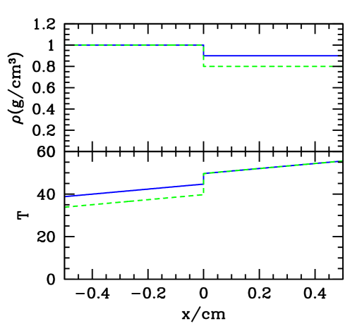
Figure 1.— Initial set-up for our Rayleigh-Taylor test simulations. Top: Initial density profile in the $\rho_{2}=0.9$ case (solid line), and in the $\rho_{2}=0.8$ case (dashed line). Bottom: Temperature profiles in both cases, with lines as in the upper panel.

As described in DT06, the growth of turbulence at the interface in this Rayleigh-Taylor unstable interface has the following analytic solution:

$$L(x,t) = L(t,0)\left[1-x^{2}/h(t)^{2}\right]^{1/2},$$ (11)

$$K(x,t) = K(t,0)\left[1-x^{2}/h(t)^{2}\right],$$ (12)

where $h(t)=\alpha_{b}A(0)t^{2}$ is a scale length for the interpenetrating fluid (with $\alpha_{b}\equiv C_{A}C_{B}/[8(1+2.C_{D})]=0.06$), and $L(t,0)=h(t)/2$ and $K(t,0)=(dh/dt)^{2}/2$ are the turbulent length scale and turbulent kinetic energy per unit mass at the interface. Following DT06, we initialize our simulation at a time of $10\mu$s and set $L(0,10\mu{\rm s})=h(10\mu{\rm s})^{2}/dx$ in the zones at either side of the interface. The resulting $K$, $L$, and density profiles are shown in Figure 2.

At all times, and for all quantities of interest, our implementation reproduces the analytic solution with a high degree of accuracy. As expected, the kinetic energy per unit mass, turbulent viscosity, and the width of the turbulent layer (taken to be the scale at which $K$ reaches a 1/10 of its maximum value) all increase as $\propto t^{2}$, which eventually leads to rapid mixing between the two materials. Furthermore, although our explicit implementation of turbulent diffusion requires us to impose a time step $\propto dx^{2}/\mu_{t}$, this works well in concert with the AMR hydro solver. As $\mu_{t}$ increases near the interface, density gradients are smoothed, allowing the code to derefine these boundaries. Thus the diffusive time step remains greater than or comparable to the one required by the Courant condition for most of the simulation, dropping only to a minimum value of about $1/6$ of the Courant time step at the very latest times, when the entire simulation volume has moved to the lowest allowed refinement value.

In Figure 3 we show the results of a similar test in which the density on the right hand side of the volume decreased to $0.8$ g/cm³, doubling the growth rate of the turbulent layer. Again, we find good agreement between our numeric approach and the analytic results, and again derefinements at late times keep the the diffusive $dt$ to manageably large values. We repeated this 2D simulation with the $x$ and $y$ coordinates interchanged, and carried out a 3D simulation in which gravity was pointed in the $z$ direction. In both cases we achieved results identical to the ones presented above.

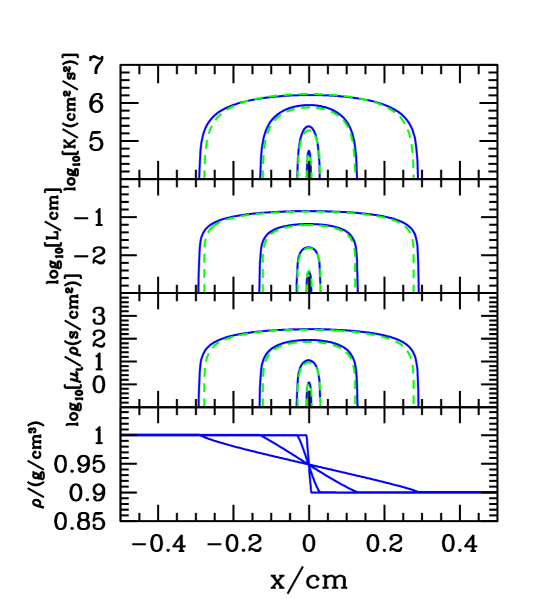
Figure 2.— Evolution in the $\rho_{2}=0.9$ case. Top: Profiles of the turbulent kinetic energy per unit mass at 50 $\mu$s, 100 $\mu$s, 200 $\mu$s, and 300 $\mu$s. In each case the solid line gives the simulation results and the dashed line gives the analytic solution. Second panel: Profiles of the turbulent length scales from the simulation (solid) and the analytic solution (dashed), with times as in the upper panel. Third Panel: Profiles of the simulated turbulent viscosity per unit mass (solid) as compared to the analytic values (dashed). Bottom: Simulated density profiles with times as in the other panels.

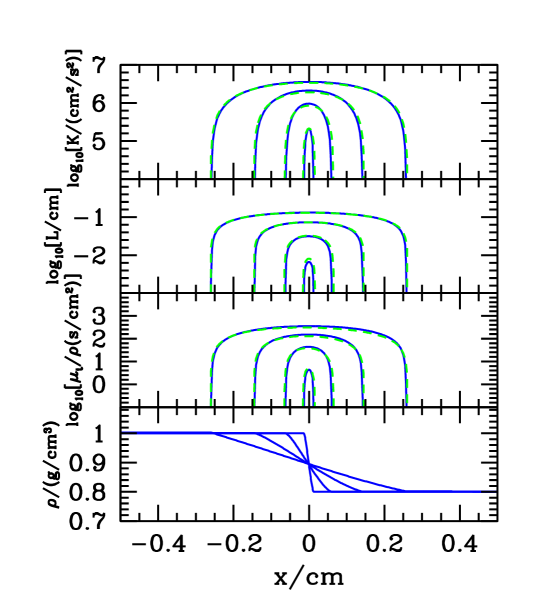
Figure 3.— Evolution in the $\rho_{2}=0.8$ case. Top: Profiles of the turbulent kinetic energy per unit mass at times of 50 $\mu$s, 100 $\mu$s, 150 $\mu$s, 200 $\mu$s, where again the solid lines give the simulation results and the dashed lines give the analytic solution. Second Panel: Profiles of the turbulent length scales with lines and times as in the upper panel. Third Panel: Profiles of the simulated and analytic turbulent viscosity per unit mass. Bottom: Simulated density profiles.

Finally, we carried out comparison runs in which we initialized the simulation as in the $x$-direction test runs, increased the resolution in the $y$ direction to 4 or 8 blocks, and turned off the subgrid turbulence model. In this case, the fluid remained stationary until perturbations from numerical errors grew to the point that fingers formed between the two materials. The delay in the onset of this stage was dependent on the resolution in the $y$ direction, and after this onset, the region containing interpenetrating fingers grew roughly as $t^{2}$.

3.2. Richtmyer-Meshkov Test

Next, we tested the ability of our code to simulate Richtmyer-Meshkov (RM) amplified turbulence (Richtmyer 1960; Meshkov 1969), which occurs when a shock encounters a discontinuity in acoustic impedance such as a density step. In this case, the shock accelerates the interface to a velocity $v_{\rm int},$ which amplifies the initial perturbations by sending the low-density regions running out ahead of the higher-density regions (e.g. Mikaelian 1989; Alon et al. 1995; Dimonte 1999; Holmes et al. 1999). As the perturbations grow and become nonlinear, the growth rate decays away in time, leading to a bubble amplitude that grows as $h_{b}\propto(v_{\rm int}t)^{\theta}_{b},$ where $\theta_{b}\approx 0.25\pm 0.05$.

To study the ability of our implementation to capture this instability, we reproduced the shock-tube test problem described in section VI of DT06. In this case, we considered a $15$ cm long region, spanning from $x=-7$ to $x=8$. The rightmost section of the simulation volume, from $x=0$ to $x=8$, was filled with a stationary gas with $\rho=0.667$ g/cm³ and $T=2.16$ K. The center region of the simulation, from $x=-6.9$ to $x=0$ was filled with a second stationary gas with $\rho=1$ and $T=1.44$ K. Both gases has a polytropic index of $\gamma=5/3$. Finally, the region from $x=-7$ to $x=-6.9$, was filled with a $\rho=1.81$ g/cm³, $T=2.27$ K, $\gamma=5/3$ gas flowing in from the left boundary at $10^{4}$ cm/s, such that a shock with a Mach number of 1.57 was established in the central gas. The simulation volume was again two-dimensional, 60 blocks in the $x$ direction by 1 block in the $y$ direction, and again 3 additional levels of refinement were allowed, such that the minimum and maximum zone size in the $x$ direction were $0.0039$ cm and $0.031$ cm respectively. Finally, along the interface we initialized $L=0.01.$

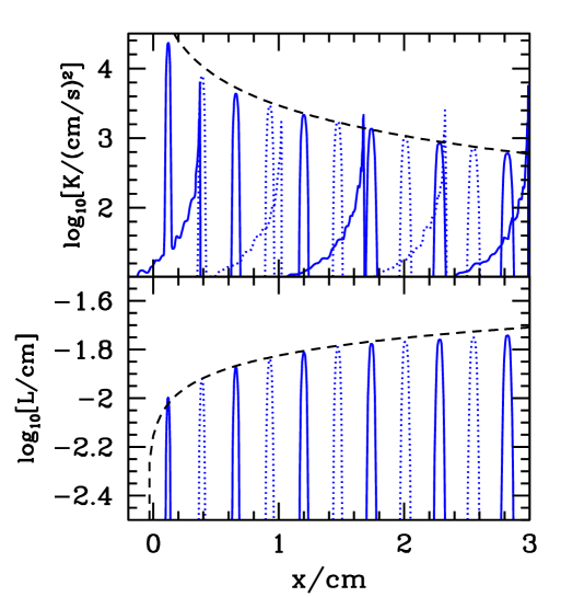
Figure 4.— Top: Profiles of the turbulent kinetic energy per unit mass at 12 outputs spaced at 25 $\mu$s intervals, beginning at the moment the shock passes through the interface. For clarity, we alternate outputs between solid lines (25 $\mu$s, 75 $\mu$s, etc.) and dotted lines (50 $\mu$s, 100 $\mu$, etc.). The dashed line shows the analytic solution for the evolution of $K$ at the interface, eq. (14). Bottom: Profiles of the simulated turbulent length scale at the time steps given in the upper panels. The dashed line shows the analytic solution, eq. (13).

For this problem the turbulent length scale and kinetic energy are expected to grow as

$$L(t) = L(0)[tv_{\rm RM}/\theta+1]^{\theta},$$ (13)

$$K(t) = K(0)[tv_{\rm RM}/\theta+1]^{2\theta-2},$$ (14)

where $\theta=(2C_{D}+1.5)^{-1}=1/4$ where $v_{\rm RM}$ is the initial post-shock time derivative of $L$ (DT06). In Figure 4 we show the $K$ and $L$ profiles that occur along the density interface as the shock passes through, as compared to these analytic solutions. Once we account for the fact that $L$ is initially compressed as the shock passes through the interface, eqs. (13) and (14), with $v_{RM}=1.6\times 10^{4}$ cm/s, give an excellent match to the simulation results. Again, we repeated this experiment interchanging the $x$ and $y$, as well as in the $z$ direction, obtaining identical results.

4. Cluster Modeling

Having carried out detailed tests of our subgrid-turbulence model, we moved on to modify FLASH3 to apply this model to the context of the AGN heated ICM. This involved choosing appropriate initial conditions and metal injection profiles, modifying the code to account for the transport and turbulent mixing of metals, and modeling AGN feedback.

4.1. Cluster Profile and Metal Injection

For our overall cluster profile, we adopted the model described in R07, which was constructed to reproduce the properties of the brightest X-ray cluster A426 (Perseus) that has been studied extensively with Chandra and XMM-Newton. In this case, the electron density $n_{\rm e}$ and temperature $T_{\rm e}$ profiles are based on the deprojected XMM-Newton data (Churazov et al. 2003; 2004) which are also in broad agreement with the ASCA (Allen & Fabian 1998), Beppo-Sax (De Grandi & Molendi 2001; 2002) and Chandra (Schmidt et al. 2002; Sanders et al. 2004) data. Namely:

$$n_{\rm e}=\frac{4.6\times 10^{-2}}{[1+(\frac{r}{57})^{2}]^{1.8}}+\frac{4.8\times 10^{-3}}{[1+(\frac{r}{200})^{2}]^{0.87}}~{}~{}~{}{\rm cm}^{-3},$$ (15)

and

$$T_{\rm e}=7\times\frac{[1+(\frac{r}{71})^{3}]}{[2.3+(\frac{r}{71})^{3}]}~{}~{}~{}{\rm keV},$$ (16)

where $r$ is measured in kpc. Furthermore, the hydrogen number density was assumed to be related to the electron number density as $n_{H}=n_{\rm e}/1.2$ according to standard cosmic abundances. The static, spherically-symmetric gravitational potential was set such that the cluster was in hydrostatic equilibrium.

The metal injection rate in the central galaxy was assumed to be proportional to the light distribution, and modeled with a Hernquist profile given by

$$\dot{\rho}_{\mathrm{metal}}(r,t)=\frac{\dot{M}_{\mathrm{metal}}{}_{0}}{2\pi}\,\frac{a}{r}\,\frac{1}{(r+a)^{3}},$$ (17)

with a scale radius of $a=10$ kpc and a total metal injection rate of $\dot{M}_{\mathrm{metal}}{}_{0}=952\,M_{\odot}\,\textrm{Myr}^{-1}.$ Note that the injection rate could also have been time-dependent, as used in Rebusco et al. (2005), to account for the higher supernova rate in the past and the evolution of the stellar population (see also Renzini et al. 1993). However, as we follow the evolution of the cluster for only about $500$ Myrs, the metal injection rate does not change significantly over this time (Rebusco et al. 2005).

Table 2Run Parameters

Run	$l_{\rm refine}$	Maximum	Effective	Subgrid	Cooling	Bubble	Bubble	Bubble	Bubble
Name		Resolution	Grid	Model		Type	Freq.	Radius	Offset
5NAES	5	0.66 kpc	$1024^{3}$	No	No	Evac.	Once	11 kpc	13.2 kpc
5DAES	5	0.66 kpc	$1024^{3}$	Yes	No	Evac.	Once	11 kpc	13.2 kpc
3NAES	3	2.6 kpc	$256^{3}$	No	No	Evac.	Once	11 kpc	13.2 kpc
3DAES	3	2.6 kpc	$256^{3}$	Yes	No	Evac.	Once	11 kpc	13.2 kpc
4NAES	4	1.3 kpc	$512^{3}$	No	No	Evac.	Once	11 kpc	13.2 kpc
4DAES	4	1.3 kpc	$512^{3}$	Yes	No	Evac.	Once	11 kpc	13.2 kpc
6NAES	6	0.33 kpc	$2048^{3}$	No	No	Evac.	Once	11 kpc	13.2 kpc
6DAES	6	0.33 kpc	$2048^{3}$	Yes	No	Evac.	Once	11 kpc	13.2 kpc
5NAES-	5	0.66 kpc	$1024^{3}$	No	No	Evac.	Once	11 kpc	13.0 kpc
5DAES-	5	0.66 kpc	$1024^{3}$	Yes	No	Evac.	Once	11 kpc	13.0 kpc
5NAES+	5	0.66 kpc	$1024^{3}$	No	No	Evac.	Once	11 kpc	13.4 kpc
5DAES+	5	0.66 kpc	$1024^{3}$	Yes	No	Evac.	Once	11 kpc	13.4 kpc
5NAES_x	5	0.66 kpc	$1024^{3}$	No	No	Evac.	Once	11 kpc	13.0 kpc
5DAES_x	5	0.66 kpc	$1024^{3}$	Yes	No	Evac.	Once	11 kpc	13.0 kpc
5NASS	5	0.66 kpc	$1024^{3}$	No	No	Sedov	Once	11 kpc	13.2 kpc
5DASS	5	0.66 kpc	$1024^{3}$	Yes	No	Sedov	Once	11 kpc	13.2 kpc
5NACR	5	0.66 kpc	$1024^{3}$	No	Yes	Evac.	50 Myr	16 kpc	17.0 kpc
5DACR	5	0.66 kpc	$1024^{3}$	Yes	Yes	Evac.	50 Myr	16 kpc	17.0 kpc
5NCSR	5	0.66 kpc	$1024^{3}$	No	Yes	Sedov	50 Myr	16 kpc	17.0 kpc
5DCSR	5	0.66 kpc	$1024^{3}$	Yes	Yes	Sedov	50 Myr	16 kpc	17.0 kpc

4.2. Tracing the metals

In order to be able to trace the metal distribution, we utilize a mass scalar to represent the local metal fraction in each cell, $F\equiv\rho_{\mathrm{metal}}/\bar{\rho}.$ Hence, the quantity $F\bar{\rho}$ gives the local metal density, $\rho_{\mathrm{metal}}$, which has a continuity equation including the metal source, given by

$$\frac{\partial{\bar{\rho}}F}{\partial t}+\frac{\partial{\bar{\rho}}F\tilde{u}_{j}}{\partial x_{j}}=\frac{\partial}{\partial x_{j}}\left(\frac{\mu_{t}}{N_{F}}\frac{\partial F}{\partial x_{j}}\right)+\dot{\rho}_{\mathrm{metal}}.$$ (18)

Furthermore, we assumed that the metal fraction is small at all times. Hence, we could neglect $\dot{\rho}_{\mathrm{metal}}$ as a source term in the continuity equation for the gas density.

4.3. Bubble generation

Bubbles in the ICM are thought to be inflated by a pair of ambipolar jets from an AGN in the central galaxy that inject energy into small regions at their terminal points, which expand until they reach pressure equilibrium with the surrounding ICM (Blandford & Rees 1974). The result is a pair of underdense, hot bubbles on opposite sides of the cluster center. As in R07 these were modeled using two methods.

In one method, we injected a total energy of $E_{\mathrm{inj}}$ over an interval of length $\tau_{\mathrm{inj}}=5\times 10^{6}$ years into each of two small spheres of radius $r_{\mathrm{inj}}$. The gas inside these spheres was heated and expanded similar to a Sedov explosion to form a pair of bubbles in a few Myrs, a time much shorter than the rise time of the generated bubbles. The parameters $r_{\mathrm{inj}}$, $E_{\mathrm{inj}}$ and $\tau_{\mathrm{inj}}$ were chosen such that these regions reached a radius of $r_{\mathrm{bbl}}$ and a density contrast of approximately $\rho_{\rm b}/\rho_{\rm amb}=0.05$ as compared to the surrounding ICM. However, the dependence of the bubble dynamics on the density contrast, $\rho_{\rm b}/\rho_{\rm amb}$, is weak provided that $\rho_{\rm b}/\rho_{\rm amb}\ll 1$ (R07). In addition to the bubbles, the explosion sets off shock waves that move through the ICM, which in fact are the energetically dominant component, as discussed in more detail below.

In another method, we evacuated the bubble regions by removing gas while keeping them in pressure equilibrium with their surroundings. Inside two spheres of radius $r_{\mathrm{bbl}}$, we removed the gas at a rate $\dot{\rho}$ for a time $\tau_{\mathrm{evac}}=5\times 10^{6}$ years that was small compared to the evolution timescale of the bubbles, but long enough to prevent numerical problems. The sink rate $\dot{\rho}$ was set to decrease the density inside the bubbles down to a density contrast of $\rho_{\rm b}/\rho_{\rm amb}$ compared to the surrounding ICM, and in order to conserve the metal mass, the metal fraction was also updated during the evacuation. Since gas was removed from a small volume in the process of forming the bubble, total mass is not conserved in this method. However, this does not affect the density profile of the cluster on the scales that we consider here. In fact, as illustrated in Fig. 4 of R07, the differences between this method and the one described above are small for the mean-flow variables. However, the evacuation method does not cause shocks that move through the ICM, making it less likely to drive further turbulence by the Richtmyer-Meshkov instability. Thus we used this model to separate out the effects of buoyancy-driven and shock-driven turbulence on galaxy clusters, and consider it first in our study. Note however that in both cases the bubble models are simplified and do not capture the details of the initial heating of the ICM by AGN jets, which can also affect stability (e.g. Sternberg & Soker 2008b)

4.4. Simulation Parameters

Recent work has considered the possibility that AGN bubbles are stabilized by molecular viscosity and magnetic fields. Reynolds et al. (2005) found that even a modest shear viscosity (corresponding to 1/4 of the Spitzer value) can quench fluid instabilities (see also Ruszkowski et al. 2004). Smoothed particle hydrodynamic simulations of buoyant bubbles in a viscous ICM were also performed by Sijacki & Springel (2006). Furthermore, it has been known for some time that the ICM hosts significant magnetic fields with typical strengths of 5 $\mu$G (Carilli et al. 2002). In many cases, the restoring tension generated by bending of the field lines may exceed the buoyancy force driving the RT instability (Chandrasekhar 1961). De Young (2003) derived analytic conditions for the stabilization by ICM magnetic fields, suggesting that observed field strengths might stabilize the bubble interface in the linear regime, and idea explored in further detail by the two-dimensional MHD calculations in Brüggen & Kaiser (2001) and recent 3D simulations by Ruszkowski et al. (2007). Yet, although viscosity and magnetic fields can clearly affect bubble dynamics and turbulence, their impact is still poorly understood, and we focus here on the basic case of turbulence arising in an inviscid and unmagnetized fluid.

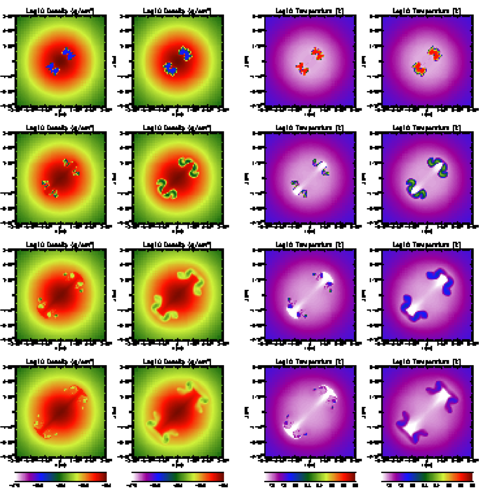
Figure 5.— Snapshots of mean-flow quantities in evacuated single-bubble runs at $t=$ 50 Myrs, 100 Myrs, 150 Myrs, and 200 Myrs (arranged from top to bottom in each column). All panels show values at a $z=0$ slice through our simulations and cover the region from $x=-100$ to 100 kpc and $y=-100$ to $100$ kpc. First Column: Contours of $\log\rho$ spanning the range from $\rho=$ $10^{-27}$ g cm^-3 to $10^{-25}$ g cm^-3 from the 5NAES pure-hydro run. Second Column: Contours of $\log\rho$ from the 5DAES run with subgrid turbulence, spanning the same range of densities as in the first column. Third Column: Contours of $\log T$ from $T=10^{7.5}$K to $10^{9}$K from the 5NAES run. Fourth Column: $\log T$ contours from the 5DAES run with the same scale as in column 3.

All our simulations are performed in a cubic three-dimensional region 680 kpc on a side, with all reflecting boundaries. For our grid, we chose a block size of $8^{3}$ zones and an unrefined root grid with $8^{3}$ blocks, for a native resolution of 10.6 kpc. The refinement criteria are the standard density and pressure criteria, and we allow for 4 levels of refinement beyond the base grid, corresponding to a minimum cell size of 0.66 kpc, and an effective grid of 1024³ zones. The parameters of all the simulations carried out in this study are summarized in Table 2. We name each run by concatenating the maximum level of refinement in FLASH3, the presence of a subgrid-turbulence model (N for none or D for DT06), whether the run uses the cooling model described below (A for adiabatic or C for cooling), the choice of bubble type (S for Sedov-Type and E for evacuated), and the whether the runs contain a single pair of bubbles (S) or periodic (P) AGN feedback.

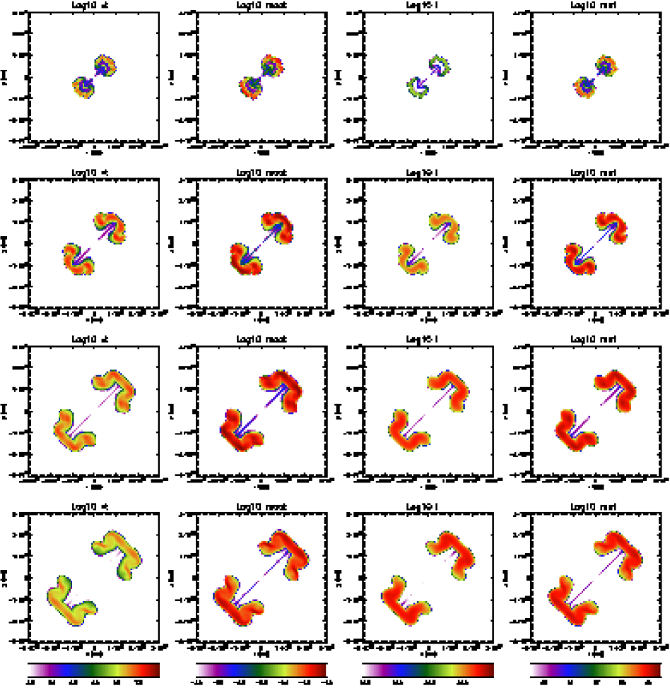
Figure 6.— Snapshots of properties of subgrid turbulence in the 5DAES run at $t=$ 50 Myrs, 100 Myrs, 150 Myrs, 200 Myrs (from top to bottom in each column). As in Figure 5, all panels show a central 200 kpc $\times$ 200 kpc $z=0$ slice. First Column: Logarithmic contours of the turbulent velocity labeled in cm s^-1 from $V=\sqrt{2K}=0.3$ km s^-1 to $V=300$ km s${}^{-1}.$ Second Column: Logarithmic contours of the local turbulent Mach number $V/c_{s}$, from $10^{-4}$ to $10^{-1}.$ Third Column: Logarithmic contours of $L$, labeled in cm, from $0.1$ kpc to $10$ kpc. Fourth Row: Logarithmic turbulent viscosity per unit density $\mu_{t}/\rho,$ labeled in cm² s^-1 from $10^{-2}$ km/s kpc to $10^{3}$ km/s kpc.

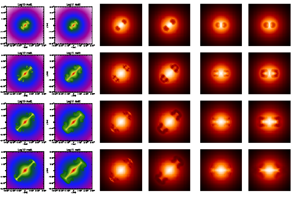
Figure 7.— Snapshots of metal and emission distribution in the central 200 $\times$ 200 kpc slice at $z=0$, at $t=$ 50 Myrs, 100 Myrs, 150 Myrs, and 200 Myrs (from top to bottom in each column) with metallicity increasing inwards. First Column: Contours of $\log\rho_{\rm metal}$ from the 5NAES run, at a fixed but arbitrary scale, with metallicity increasing inwards. Second Column: Contours of $\log\rho_{\rm metal}$ from the turbulence run, with a scale matching the first column. Third Column: Unsharp X-ray image from the 5NAES run, projected in the $z$-direction. Fourth Column: Unsharp X-ray image from the 5DAES run, projected in the $z$-direction. Fifth Column: Unsharp X-ray image from the 5NAES run, projected in the $x$-direction. Sixth Column: Unsharp X-ray image from the 5DAES run, projected in the $x$-direction.

5. Results

5.1. Evacuated Bubbles

As our first case study, we carried out two simulations: an adiabatic pure-hydro simulation (5NAES) and an adiabatic simulation with subgrid turbulence (5DAES). At the start of each simulation a single pair of $r_{\rm bubble}=11$ kpc bubbles was centered along the $x=y$ axis at an offset of $R_{0}=\pm 13.2$ kpc, and within the bubbles the gas was evacuated to $\rho_{b}/\rho_{\rm amb}=0.05$ and heated to 20 times the temperature of the surrounding medium. Snapshots of density and temperature from these simulations appear in Figure 5, spanning times from 50 to 200 Myrs.

The differences between the two runs are dramatic. In the pure-hydro run the bubbles fragment after rising a single pressure scale height. The dominant unstable modes that are set by the resolution of the adaptive grid quickly shred the evacuated regions, drastically reducing them in size. If we were able to repeat this simulation with arbitrarily high resolution, we would find that the bubbles have developed fingers upon fingers of turbulence, which penetrate deep into the surrounding medium. However, this dispersal is halted by the finite resolution in the pure-hydro run, which by 100 Myrs has already significantly underestimated the mixing between the evacuated region and its surroundings.

On the other hand, the subgrid-turbulence run captures this mixing, modeling the growth of all the modes that our computational grid cannot resolve. The superposition of these modes then smears out the interface between the bubble and the ambient medium, transforming the bubbles into clouds of mixed material, which stay intact and expand as they rise in the stratified ICM. Note that in both runs the bubbles are trailed by streams of colder gas, which are lifted from the center and cool adiabatically, consistent with observations (e.g. Simionescu et al. 2007).

To quantify the properties of the turbulent clouds further, in Figure 6 we plot slices from our 5DAES simulation, focusing on quantities evolved by the subgrid model. Turbulent velocities quickly approach a maximum of $\approx 100$ km s${}^{-1},$ roughly $5\%$ of the sound speed within the bubbles and $10\%$ of the sound speed of the surrounding ICM. As the hot gas rises at $\approx 500$ km/s, the turbulent motions are fast enough to mix this material with the surrounding medium, but much too slow to halt its overall motion. In addition to the velocity of turbulent motions, the efficiency of this mixing process is dependent on the scale of the turbulent eddies, which is plotted in the third column of Figure 6. Here we see that $L$ quickly rises to $\approx 10$ kpc, but does not exceed the overall size of the clouds, keeping material well-mixed within these $\approx 30$ kpc regions. Together $L$ and $V$ act to produce a typical turbulent viscosity of $\approx 300$ km/s kpc, which diffuses material between the clouds and their surroundings. Thus rather than being a destructive process, turbulence acts as an effective mixing mechanism, which alters the rising structure, but operates at scales that are too small and with velocities that are too slow to disrupt it completely.

To study this mixing process further, we compare the distribution of ICM metals from our 5DAES (subgrid-turbulence) and 5NAES (pure-hydro) simulations in the left two columns of Figure 7. In both runs, highly-enriched material from the center of the cluster is carried outward by the rising bubbles, but this transport is much more effective in the 5DAES run. In the pure-hydro run metal transport is halted at $\approx 50$ kpc by bubble disruption, which occurs when RT instabilities shred the evacuated region into resolution-limited cavities. In the subgrid-turbulence run, on the other hand, small-scale fluctuations act to move metals into the cloud while at the same time keeping the structure coherent, such that it continues to rise out to substantially larger radii.

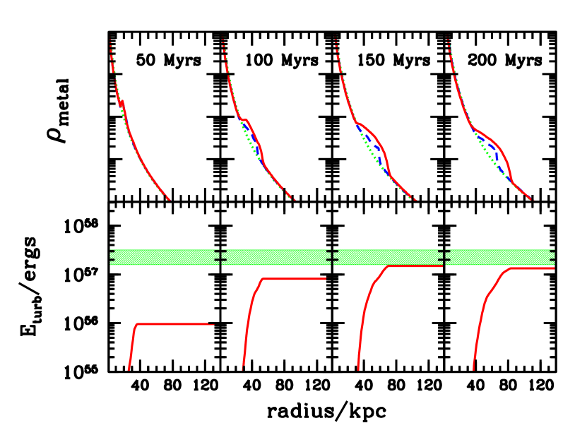
Figure 8.— Metal density and total turbulent kinetic energy at times of 50 Myrs, 100 Myrs, and 150 Myrs, 200 Myrs arranged in columns from left to right. Top: Metal density from the evacuated-bubble subgrid-turbulence run (5DAES, solid lines), and from the evacuated bubble pure-hydro run (5NAES, dashed lines). For comparison the dotted line shows the Hernquist profiles in which metal are ejected into our simulations. The logarithmic scale in this row is fixed, but arbitrary. Bottom: Total turbulent kinetic energy contained within a given radius, as a function of that radius (solid lines). The shaded regions are bounded by 1% to 2% of $E_{\rm bouyancy}$ as given by eq. (19).

We quantify this in the upper row in Figure 8, which shows the overall density of metals as a function of radius in each of our runs. By 150 Myrs, the bubbles in the 5NAES run have dissipated, leaving behind substantial enhancement of metals within 50 kpc, but having little or no impact outside of this radius. On the other hand, clouds in the subgrid-turbulence run continue to rise even at 200 Myrs, leading to enhancements of by over a factor of 5 at 70 kpc.

In the lower panel of Figure 8 we plot $E_{\rm turb}$, the total turbulent kinetic energy within a given radius in our 5DAES simulation. This can be directly compared with the total energy available from the buoyant rise of the bubbles, which can be simply estimated as (e.g. Nulsen et al. 2006)

$$E_{\rm bouyancy}\approx\int_{R_{0}}^{\infty}V(R)\frac{dp}{dR}dR\approx\frac{3p_{\rm evac}V_{\rm evac}}{2},$$ (19)

where $R$ is the distance of the bubble from the center of the cluster which is initially at $R_{0}.$ This gives a value of $\approx 10^{59.2}$ ergs per pair of $r_{\mathrm{bbl}}=11$ kpc bubbles. Comparing this value to the turbulent kinetic energy in our simulations, we find that $E_{\rm turb}$ is only $\approx 1\%$ of this overall energy, thus we do not expect the energy of the turbulent motion themselves to play a major role in the heating of the cool-core region in the ICM. Rather, the key impact of turbulence is to increase the efficiency with which the thermal energy of the rising cloud is mixed into its surroundings (e.g. Soker 2004; Sternberg et al. 2007; Sternberg & Soker 2008b). In this sense it behaves much more like heat conduction (e.g. Narayan & Medvedev 2001; Voigt & Fabian 2004; Ruszkowski et al. 2004; Sternberg et al. 2007), than an energy source. Note however, that our simple turbulence model does not account for shear-driven effects, and thus may somewhat underestimate $E_{\rm turb},$ though not by orders of magnitude.

Finally, the physical differences between the two runs lead to different observed morphologies. In the right panels of Figure 7 we present approximate X-ray images from each of the two runs, calculated by projecting the emissivity, computed as

$$\epsilon=\Lambda(T)n_{e}^{2},$$ (20)

where we estimate the cooling function, $\Lambda(T),$ which describes radiative losses from the optically-thin plasma, as in Sarazin (1986; see also Raymond et al. 1976; Peres et al. 1982). Furthermore, to draw out structure we create unsharp mask images by dividing the map by a 30 kpc smoothed version of itself.

These images are comparable to those in the study by Reynolds et al. (2005), which was carried out with similar resolution, but in a hydrostatic atmosphere falling off as $\rho(r)\propto[1+(r/r_{0})^{2}]^{-0.75},$ which is significantly less steep than the one we have prescribed in the central cooling flow region of our simulation. Furthermore our times can easily be related to their dimensionless units as $t=\tilde{t}\times 57{\rm kpc}/c_{s}\approx\tilde{t}$ 60 Myrs. Our 5NAES run thus confirms the Reynolds et al. (2005) result that pure-hydro inviscid bubbles fall apart within a dimensionless time of $\tilde{t}=3$, or $\approx$ 200 Myrs, although our steeper radial slope combined with our processing of the image is able to draw out more structure than visible in their plots. It is clear that these collections of fragments look nothing like the smooth and detached cavities of the type observed in Perseus (e.g. Fabian et al. 2006) and other clusters (e.g. McNamara et al. 2001; Choi et al. 2004; Reynolds et al. 2008). On the other hand, in the subgrid-turbulence run, the hot clouds lead naturally to coherent holes in the X-ray distribution not unlike those observed in cool-core clusters. If anything the bubbles are too large and radially extended as compared to observations, an issue we take up below, after first addressing the reliability of our numerical approach.

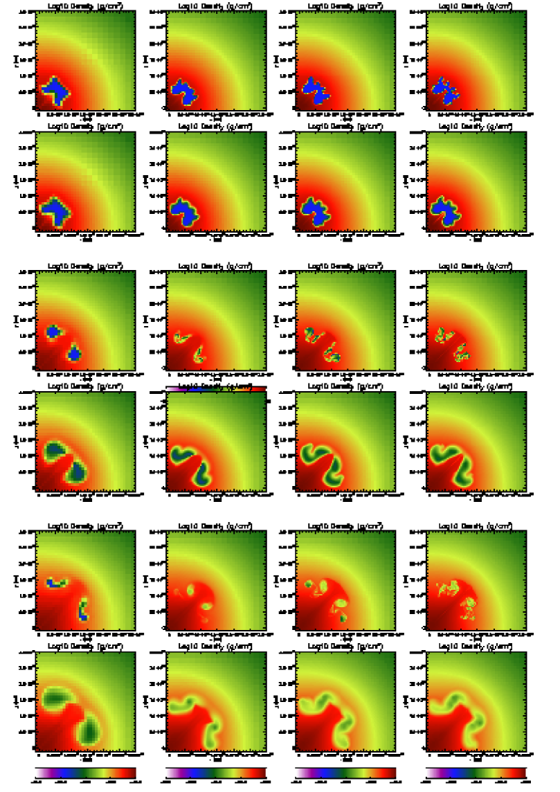
Figure 9.— Snapshots of $\log\rho$ in single-bubble runs of varying resolution. Plots show a $z=0$ slice of the region from $x=-3$ kpc to $100$ kpc and and $y=-3$ kpc to $100$ kpc from the pure-hydro run. From left to right, each column shows results from simulations with 3 levels of refinement (2.6 kpc resolution), 4 levels of refinement (1.3 kpc resolution), the fiducial 5 levels of refinement (0.66 kpc resolution), and 6 levels of refinement (0.33 kpc resolution). Top Row: Outputs at 50 Myrs from runs without the subgrid-turbulence model. Second Row: Outputs at 50 Myrs from runs including subgrid turbulence. Third Row: Outputs at 100 Myrs from runs without subgrid turbulence. Fourth Row: Subgrid-turbulence run outputs at 100 Myrs. Fifth Row: Outputs at 150 Myrs from runs without subgrid turbulence. Sixth Row: Subgrid-turbulence run outputs at 150 Myrs.

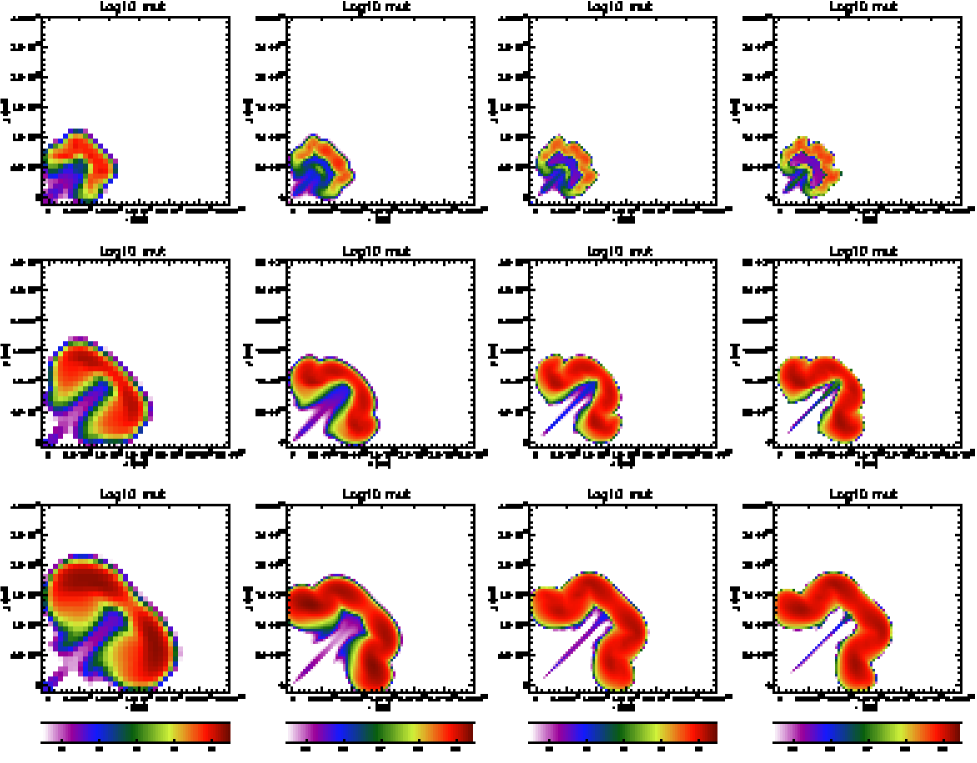
Figure 10.— Snapshots of the turbulent viscosity per unit density, $\log\mu_{t}/\rho,$ in single-bubble runs of varying resolution. As in Figure 9, plots show a $z=0$ slice of the region from $x=-3$ kpc to 100 kpc in the $x$ and $y$ directions, and from left to right, each column shows results from simulations with $l_{\rm refine}=3$ (2.6 kpc resolution), $l_{\rm refine}=4$ (1.3 kpc resolution), the fiducial $l_{\rm refine}=5$ case (0.66 kpc resolution), and $l_{\rm refine}=6$ (0.33 kpc resolution). From top to bottom, each row shows outputs at 50 Myrs, 100 Myrs, and 150 Myrs respectively. In all panels $\mu_{t}/\rho$ is labled in units of cm² s^-1 and goes from from $10^{-2}$ km/s kpc to $10^{3}$ km/s kpc.

5.2. Dependence on Resolution and Initial Parameters

An important issue in any simulation is the degree to which its results are modified when one changes the minimum zone size. This is of particular concern here, because the DT06 model must evolve all subgrid modes contributing to the RT instability, while still achieving results that are resolution-independent. With this in mind, we carried out a set of convergence tests, repeating our simulations with and without the subgrid model for cases in which we varied the maximum level of refinement from $l_{\rm refine}=3$ (2.6 kpc resolution, $256^{3}$ effective grid) up to $l_{\rm refine}=6$ (0.33 kpc, $2048^{3}$ effective grid). Snapshots from these simulations are presented in Figure 9, in which we have zoomed into the area from $x=-3$ kpc to 100 kpc, and $y=-3$ kpc to 100 kpc to emphasize the regions that are most affected by turbulence.

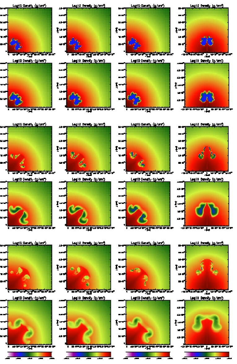
Figure 11.— Snapshots of $\log\rho$ in single-bubble runs with slightly different initial conditions. As in Figure 9, plots show a $z=0$ slice of the region from $x=-3$ kpc to $100$ kpc and and $y=-3$ kpc to $100$ kpc. From left to right, each row shows results from simulations in which the bubbles have been initially moved radially by $-1\%$, $0\%$, $1\%$, and respectively. Finally, the rightmost row show a run in which the bubbles are placed along the $y$ axis. Top Row: Outputs at 50 Myrs from runs without the subgrid-turbulence model. Second Row: Outputs at 50 Myrs from runs including subgrid turbulence. Third Row: Outputs at 100 Myrs from runs without turbulence. Fourth Row: Turbulence run outputs at 100 Myrs. Fifth Row: Outputs at 150 Myrs from runs without turbulence. Sixth Row: Turbulence run outputs at 150 Myrs.

Focusing first on the pure-hydro runs at 50 Myrs, one sees a clear increase in small-scale structure as the runs progress to higher resolution. The wavelength of the fastest growing mode from a linear analysis of the RT instability is given by (Chandrasekhar 1981)

$$\lambda_{\rm max}=4\pi(\nu^{2}A/g)^{1/3},$$ (21)

where $A$ is the Atwood number, $g$ is the gravitational acceleration, and $\nu$ is the viscosity of the fluid, which, in the pure-hydro run, is given by the effective numerical viscosity. In the PPM method used by FLASH, the dissipative processes that act as an effective $\nu$ are extremely nonlinear. Not only are the error terms in this high-order scheme extremely complicated, but they change with the nature of the flow, as PPM uses several switches that detect discontinuities (Woodward & Colella 1984; Porter & Woodward 1994). Thus the effective $\nu$ value in our simulations is dependent on the structures we are trying to resolve, and is best expressed as an effective Reynolds number $Re=d\,v/\nu,$ where $d$ and $v$ are the size and the velocity of the structure of interest.

For our fiducial simulations (with $l_{\rm refine}=5$) the effective number of zones is $1024^{3},$ which corresponds to a spatial resolution of 0.66 kpc. In the case of large subsonic eddies, not unlike our bubbles, detailed studies have shown the effective Reynolds number achievable in PPM simulations is proportional to the number of grid points across the fluctuation of interest to the power of $N=3$, where $N$ is the order of the numerical scheme (Porter & Woodward 1994; Balbus et al. 1996; Sytine et al. 2000). In their study of viscous bubbles, Reynolds et al. (2005) carried out a series of runs in which numerical viscosity was explicitly added to the system at different levels, and they determined that FLASH3 behaved roughly as if $Re\approx 2000-5000.$ Using this number as a rough guide in our fiducial case, which again has resolution similar to that in Reynolds et al. (2005), this implies that the numerical viscosity is of the order of

$$\nu\sim d\,v/{\rm Re}\sim 3\,{\rm km\,s}^{-1}\,{\rm kpc},$$ (22)

where we assumed $d\approx 25$ kpc and $v\approx 500$ km/s. Taking this $\nu$ value, along with $A\approx 1$ and $g\approx 10^{-8}$ cm s^-1, this yields a fastest growing mode wavelength of $\lambda_{\rm max}\approx 2$ kpc, which roughly corresponds to the scale of the small features seen in the fiducial pure-hydro run at 50 Myrs.

From eq. (21), and assuming that viscosity goes as the number of grid points to the power of 3, $\lambda_{\rm max}\propto l_{\rm refine}^{-2}$. Thus decreasing the resolution to $l_{\rm refine}=4$, which corresponds to a spatial resolution of $1.3$ kpc, moves $\lambda_{\rm max}$ up to $\approx 8$ kpc, greatly reducing the perturbations seen at 50 Myrs. Similarly, choosing $l_{\rm refine}=3$ moves $\lambda_{\rm max}$ up to the scale of the bubbles, and no perturbations are visible. On the other hand, in the $l_{\rm refine}=6$ run, $\lambda_{\rm max}$ is reduced almost to the resolution limit, leading to perturbations on all simulated scales. At later times, the differences between runs persist, such that the bubbles are shredded into subclumps with sizes that are strongly resolution-dependent. Note however, that the fastest growing mode as given by eq. (21), need not be precisely the mode that dominates the late-time nonlinear evolution of the subclumps, as the growth of perturbations at $\lambda_{\rm max}$ may saturate.

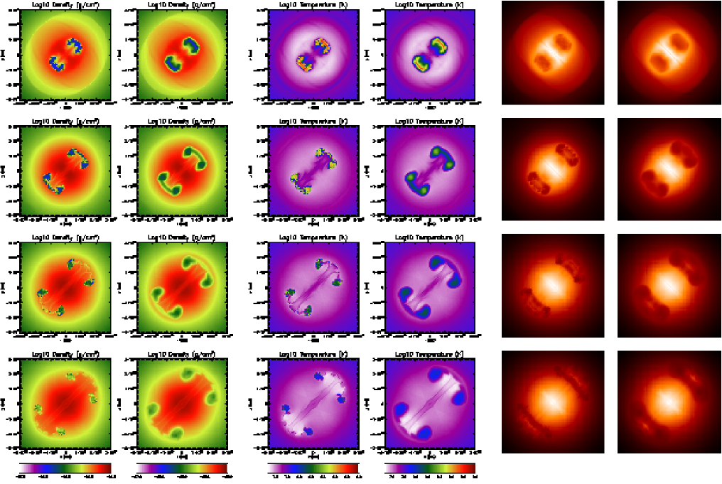
Figure 12.— Snapshots of mean-flow quantities in Sedov single-bubble runs at 50 Myrs, 100 Myrs, 150 Myrs, 200 Myrs (arranged from top to bottom in each column). All panels show values at a $z=0,$ slice through our simulations and cover the region from $x=-100$ to 100 kpc and $y=-100$ to $100$ kpc, with scales chosen as in previous plots. First Column: Contours of $\log\rho$ from the run without subgrid turbulence, spanning the range from $\rho=$ $10^{-27}$ g cm^-3 to $10^{-25}$ g cm${}^{-3}.$ Second Column: Contours of $\log\rho$ from a run with subgrid turbulence, and spanning the same range of densities as in the upper panels. Third Column: Contours of $\log T$ from $T=10^{7.5}$K to $10^{9}$K, from the run without subgrid turbulence. Fourth Column: $\log T$ contours from the turbulence run, again with the same dynamical range. Fifth Column: Unsharp X-ray image from the 5NASS run, projected in the $z$-direction. Sixth Column: Unsharp X-ray image from the 5DASS run, projected in the $z$-direction.

Moving to the subgrid model runs, we find no such dependence on resolution. In this case, the code carries two additional quantities, namely the turbulent length scale, $L$, and kinetic energy, $K$. It evolves $L$ and $K$ to reproduce the analytic growth of the RT and RM perturbations in the limit in which the molecular viscosity is small and does not play a role on the scales of interest. The growth of small-scale perturbations is then completely captured by the evolution of $L$ and $K,$ which are used to construct a turbulent viscosity that is imposed on the mean-field variables explicitly. The role of the numerical viscosity in eq. (21) is then played by $\mu_{t}/\rho,$ which grows to a value of 300 km/s kpc, larger than the numerical viscosity in all of the runs. Thus rather than breaking up into a collection of resolution-dependent subgroups, the mean-field density distributions remains coherent, while at the same time the simulation is able to maintain the information necessary to calculate the mixing of the turbulent material with the surrounding medium.

Furthermore, the evolution of the turbulent viscosity is determined by the overall properties of the flow, and is largely independent of resolution. A test of this convergence is shown in Figure 10, which gives snapshots of $\log\mu_{t}/\rho$ in each of our single-bubble runs with varying resolution. Here we see that $\mu_{t}/\rho,$ whose evolution is determined by the gravitational acceleration and the Atwood number, evolves to $\approx 300$ km/s kpc regardless of our choice of $l_{\rm refine}.$ Thus the overall structure of evolving bubbles is quite similar across runs.

The subgrid-turbulence model also greatly reduces the sensitivity of our results on the detailed choice of initial conditions. Figure 11 shows the results of pure-hydro and subgrid simulations in which we have taken the initial offset of the bubbles to be $R_{0}=13.0$, $13.2$, and $13.4$ kpc, as well as a pair of runs in which we have taken $R_{0}=13.0$ kpc, but oriented along the $y$-axis. In the pure-hydro case, our results show a strong sensitivity to these $\pm 2\%$ changes in initial position. This is because the code is attempting to sample an underlying turbulent density field with resolution-dependent subclumps, whose locations vary significantly depending on the nonlinear, position- and velocity-dependent effective numerical viscosity. In the subgrid runs however, the presence of the turbulent viscosity leads to a smoothing over the unresolved turbulent density distribution, thus capturing the full range of positions over which fully-resolved turbulent material would be spread.

5.3. Sedov Bubbles

Next we turned our attention to the more computationally-demanding case in which the bubbles are modeled as initially overpressured spheres. In this case we raised the internal temperature such that each bubble expanded to a density of $\rho_{b}/\rho_{\rm amb}=0.05$ before reaching pressure equilibrium with a bubble size equal to the one in the evacuated model. For a $\gamma=5/3$ gas, the energy input during this expansion can be simply calculated as

$$E_{\rm expand}=\int_{V_{\rm init}}^{V_{\rm evac}}dVp=\frac{3p_{\rm final}V_{\rm evac}}{2}\left[\left(\frac{V_{\rm evac}}{V_{\rm init}}\right)^{2/3}-1\right],$$ (23)

where $p_{\rm evac}$ and $V_{\rm evac}$ are the pressure and volume at the evacuated stage at the end of the expansion and $V_{\rm init}$ is the initial volume. Although the bubble expansion occurs at approximately the sound speed of the internal material, this velocity is well above to the sound speed of the exterior gas. This energy is then deposited into shocks which act both to directly raise the temperature in the surrounding medium, as well as increase the turbulent kinetic energy through the Richtmyer-Meshkov instability as the shocks meet acoustic discontinuities. This energy input can be contrasted to the energy input from the buoyant motions of the bubbles studied in §5.1, as given by eq. (19). For our choice of $\rho_{b}/\rho_{\rm amb}=0.05$, $\left(V_{\rm evac}/V_{\rm init}\right)^{2/3}-1=6.35$. Thus $E_{\rm expand}/E_{\rm buoyancy}\approx 6$, such that overpressured bubbles should have a significantly greater impact on the cluster than the evacuated model.

The impact of this energy is seen in the outer oval-shaped shock visible in the 50 Myr plots of density, temperature, and simulated X-rays shown in Figure 12. Trailing behind this discontinuity is a second density and temperature jump, which is due to initially inward-facing shocks that reflect off each other and move into the surrounding medium. The motion of these reflected shocks through the rising bubbles has a noticeable effect on the bubbles’ morphology, substantially compressing them in the radial direction. At later times in the pure-hydro run, the result is a flattened distribution of distinct cavities, which separate and shred as the bubbles move outwards, much as they did in the 5NAES simulation.

In the subgrid-turbulence case, however, the result is a flattened but coherent cloud which moves outwards, mixing with the surrounding medium while remaining intact. This distinctive shape immediately brings to mind familiar images of the “mushroom cloud” structure that results from a large airburst in the atmosphere of Earth. Indeed, the language used to describe such clouds, such as a “toroidal fireball” perched atop a somewhat cooler updrafting “stem,” (e.g. Glasstone & Dolan 1977), translates naturally to describe the structures we see in our simulations. In fact, the physics of these two phenomena are deeply connected. In both cases an unstable bubble is rising upward in a hydrostatic medium. In both cases this bubble is neither stabilized by magnetic fields nor through viscosity. And in both cases the hot gas is well-mixed with the surrounding medium as it moves through it, yet it manages to retain its shape. Furthermore, as shown in the rightmost panels of Figure 12, these radially-flattened clouds lead naturally to X-ray “holes” of precisely the type observed in cool-core clusters, without requiring additional physics.

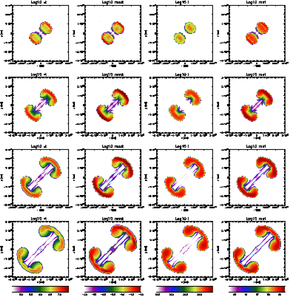
Figure 13.— Snapshots of properties of subgrid turbulence in the Sedov single-bubble (5DASS) run at $t=$ 50 Myrs, 100 Myrs, 150 Myrs, 200 Myrs (from top to bottom in each column). All panels show a central $z=0$, 200 kpc $\times$ 200 kpc slice. First Column: Logarithmic contours of the turbulent velocity from 0.1 km s^-1 to 100 km s${}^{-1}.$ Second Column: Logarithmic contours of the local turbulent Mach number from $10^{-4}$ to $10^{-1}$ Third Column: Logarithmic contours of $L$ from $0.1$ kpc to $10$ kpc. Fourth Row: Logarithmic turbulent viscosity per unit density from $10^{-2}$ km/s kpc to $10^{3}$ km/s kpc.

In Figure 13 we show the evolution of the turbulence variables in the 5DASS run. In general, the turbulent velocities and length scales are systematically enhanced with respect to the evacuated-bubble run, due to the effect of the RM instability. In this case, turbulent velocities can approach 300 km/s, 50% greater than 5DAES run, but still well below the $\approx 500$ km/s radial velocity of the cloud. Similarly, the turbulent length scales grow faster at early times and remain somewhat higher at later times, as compared to the evacuated case, but they never exceed the overall scale of the rising cloud. Together $V$ and $L$ act to generate a typical turbulent viscosity of $10^{3}$ km/s kpc, a substantial value that is likely to significantly influence the overall evolution of the intracluster medium.

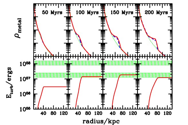
Figure 14.— Metal density and turbulent kinetic energy (bottom row) from the Sedov single-bubbles runs at times 50 Myrs, 100 Myrs, and 150 Myrs, 200 Myrs arranged in columns from left to right. Top: As in Figure 8, the solid lines are drawn from the subgrid-turbulence run (5DASS), the dashed lines are from the pure-hydro run (5NASS), and the dotted line is the profile in which metals are injected. Bottom: Total turbulent kinetic energy within a given radius in our simulations (solid lines) contrasted with 1-2% of $E_{\rm bouyancy}$ and 1-2% of $E_{\rm expand}+E_{\rm bouyancy},$ represented by the lower and upper shaded regions, respectively.

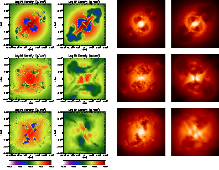
Figure 15.— Snapshots of mean-flow quantities in the periodic evacuated-bubble runs at 150 Myrs, 300 Myrs, and 450 Myrs (arranged from top to bottom in each column). All panels show values at a $z=0$ slice through our simulations and cover the region from $x=-100$ to 100 kpc and $y=-100$ to $100$ kpc, with scales chosen as in previous plots. First Column: Contours of $\log\rho$ from the run without subgrid turbulence, spanning the range from $\rho=$ $10^{-27}$ g cm^-3 to $10^{-25}$ g cm${}^{-3}.$ Second Column: Contours of $\log\rho$ from a run with subgrid turbulence, and spanning the same range of densities as in the upper panels.Third Column: Unsharp mask X-ray image from the 5NCER run, projected in the $z$-direction. Fourth Column: Unsharp mask X-ray image from the 5DCER run, projected in the $z$-direction.

In Figure 14 we quantify the radial distribution of metals and turbulent energy in our Sedov-bubble simulations. In this case the differences in $\rho_{\rm metal}$ between the pure-hydro and subgrid-turbulence runs are much less dramatic than they were in the evacuated-bubble models. The overall shock heating of the central region drives metals outwards to $\approx 80$ kpc in 200 Myrs, regardless of whether they are transported in well-mixed clouds or fragmented cavities. A comparison of $E_{\rm turb}$ to the energy from the buoyant bubbles shows that while the Richtmyer-Meshkov instability increases turbulence somewhat from the evacuated case, the magnitude of this change is much smaller than the factor of $\approx 7$ increase in available energy. Most of the excess energy instead goes directly into post-shock heating or establishing large-scale motions. Thus even more than in the evacuated case, turbulence plays a role primarily in determining mixing and structure, rather than in providing a source of energy to balance cooling.

5.4. Periodic Bubbles

Finally, we carried out a set of simulations to study the impact of our subgrid-turbulence models on the evolution of cool-core clusters on longer time scales. This involved two major changes from our single-bubble simulations.

First, we implemented a model in which AGN-driven bubbles occur periodically, again following an approach developed in R07. As in our previous runs, we generated bubbles in pairs, but now at regular intervals of $\tau_{\mathrm{bbl}}=50$ Myrs. Furthermore, we rotated the position of the center of the bubble pairs by 90 degrees around the $y$-axis. Thus, the first pair of bubbles was centered at $z=0$ and $x=y=\pm R_{0}/\sqrt{2}$, the second pair of bubbles at $x=0$ and $y=z=\pm R_{0}/\sqrt{2},$ the third at $z=0$ at $x=-y=\pm R_{0}/\sqrt{2}$, etc., cycling back to the original position every 200 Myrs.

The second major change to our simulations was the addition of cooling, which was calculated in the optically-thin limit from the same emissivity as used to construct our X-ray images, namely $\epsilon=\Lambda(T)n_{e}^{2}$, where the cooling function $\Lambda(T)$ was taken from Sarazin (1986). However, in order to avoid drastic cooling within a single timestep we did not cool cells in which the density was above $5\times 10^{-25}$ g cm^-3 or in which the temperature was below $5\times 10^{6}$K. This placed an absolute entropy floor in our simulations at 5 keV cm².

With this cooling in place, we found that our simulation was initially radiating at $\approx 4\times 10^{44}$ ergs per second or $\approx 1.2\times 10^{60}$ ergs per 100 Myrs. Thus we chose to scale up our bubbles to a radius of $r_{\mathrm{bbl}}=16$ kpc such that $E_{\rm buoyancy}\approx 5\times 10^{59}$ ergs, and the energy input from buoyant heating roughly balanced cooling. As before, the parameters for our runs are summarized in Table 2.

Figure 15 shows snapshots of these simulations in the evacuated-bubble case at times of 150, 300, and 450 Myrs. Like the single-bubbles runs, the pure-hydro simulation (5NCER) shows significantly more fragmentation than the subgrid turbulence run (5DCER), particularly towards the outskirts of the cluster. However, unlike the single-bubble runs, the properties of the two simulations continue to diverge with time at all radii. This is because turbulence driven by previous feedback events remains behind, enhancing the mixing of subsequent bubbles.

Thus, at late times, the X-ray maps from the subgrid-turbulence run contain two prominent holes, while the distribution in the pure-hydro run is much more fragmented. Note also that by 450 Myrs, errors introduced by the split-hydro solver employed by FLASH3 have grown to the point that substantial assymetries are seen in the pure-hydro runs. As we saw in Figure 11 this dependence on small fluctuations is reduced in the subgrid turbulence run, as the turbulence viscosity smoothes over what are essentially different realizations of the same turbulent density field, a field that has been unnaturally quantized into resolution-dependent subclumps in the pure-hydro runs.

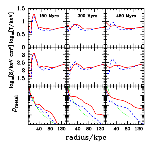
Figure 16.— Radial profile of mean-flow quantities in evacuated periodic bubble runs at times of 150 Myrs, 300 Myrs, and 450 Myrs, arranged in columns from left to right. From top to bottom, the rows show the average temperature, entropy, and metal density. In all panels the solid lines are taken from the subgrid-turbulence run (5DCER) and the dashed lines are taken from the pure-hydro run (5NCER). The dotted lines in the bottom panels show the metal profile that would be found if there were no resolved or subgrid velocities in the simulations.

Figure 16 shows the evolution of the radial profiles of mean-field quantities in our simulations. Focusing first on temperature, clear differences are apparent between the two runs, and these differences grow stronger with time. Within the central 20 kpc the temperature in the subgrid-turbulence run is roughly a factor of two greater than in the pure-hydro run, and a similar difference is apparent in the radial entropy profile. As suggested by the single-bubble runs, and as quantified for the 5DCER run below, these differences are not due to additional energy input from dissipated turbulent kinetic energy. Rather, the primary role of turbulence is to improve the mixing of the thermal energy from the interior of the heated cavities into the surrounding cold gas (e.g. Soker 2004; Sternberg et al. 2007). This means that while in the pure-hydro run, the bubbles deposit most of their internal energy at the resolution-dependent radius at which they get disrupted, as indicated by the spike in temperature at $R\approx 30$ kpc. Hence, the turbulent motions captured by the subgrid model cause much more gradual heating, which leads to shallow temperature and entropy profiles at all radii $\leq 30$ kpc.

At the same time, the well-mixed clouds in the subgrid-turbulence run remain coherent to larger radii, increasing the sphere of influence over which AGN-driven heating is effective. This can be clearly seen in a comparison of the metal profiles between the two runs, which indicates enhancement of almost an order of magnitude in the subgrid-turbulence runs relative to the pure-hydro runs, an enhancement which is particularly strong at large radii, but significant even in the central regions of the cluster.

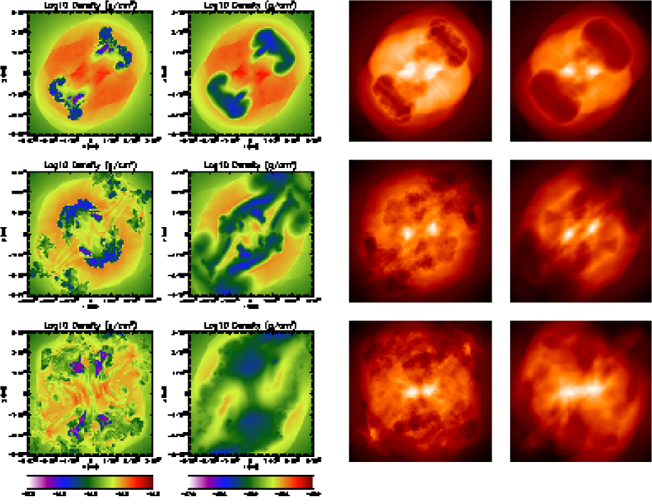
Figure 17.— Snapshots of mean-flow quantities in the periodic Sedov bubble runs at 100 Myrs, 200 Myrs, and 300 Myrs (arranged from top to bottom in each column). Panels and symbols are as in Figure 15.

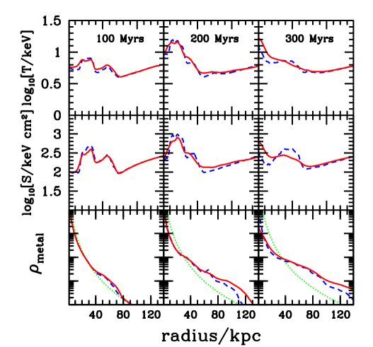
Figure 18.— Radial profile of mean-flow quantities in Sedov multiple-bubble runs at times of 100 Myrs, 200 Myrs, and 300 Myrs, arranged in columns from left to right. From top to bottom the rows show the average temperature, entropy, and metal density. Symbols are as in Figure 16.

Turning to the Sedov-bubble case, similar trends are apparent. Here, an extremely large number of AMR zones were necessary at late times ($\approx 10^{5}$ blocks of $8^{3}$ zones each), forcing us to end our simulations at 300 Myrs. However, the density slices and X-ray images presented in Figure 17 over this time period paint a similar picture to the evacuated-bubble runs. Again the build-up of turbulent motions over time causes the properties of the two simulations to diverge. Again this increase in mixing is especially notable near the core, where a large number of small fragments in the pure-hydro case are replaced by an overall smooth and quadrapole-like configuration in the subgrid-turbulence run. And again the subgrid model serves to damp out much of the chaotic amplification of small assymetries. Furthermore, the X-ray images of the subgrid turbulence runs show larger and smoother cavities, although interestingly, the pure-hydro runs contain significant associations of shredded bubble material that appear as coherent X-ray depressions, albeit somewhat more ragged depressions than are seen in the observations.

As in the evacuated-bubble case, the radial profiles plotted in Figure 18 show that subgrid turbulence leads to more efficient heating in the central $R\leq 30$ kpc core. On the other hand, at larger radii heating is dominated by shocks and is similar between the two runs. Note that as $E_{\rm expand}$ is substantially greater than $E_{\rm buoyancy}\approx E_{\rm cool},$ these simulations show an overall increase in the central temperature and entropy of the cluster at late times. In reality, entropy is unlikely to rise beyond the point at which the cooling near the core becomes inefficient, as this would halt gas accretion onto the central black hole and the further creation of bubbles. Accounting for this change in gas accretion rate would lead to a self-regulating configuration (e.g. Voit & Bryan 2001; Bîrzan et al. 2004; McNamara & Nulsen 2007; Voit et al. 2008) whose modeling falls beyond the scope of our study here.

In the lower panels of this figure, we plot the metal profiles between the two runs. Although metal mixing is somewhat more efficient at larger radial in the subgrid-turbulence run, the metal profiles are much more similar between the two runs than they were in the the evacuated-bubble case.

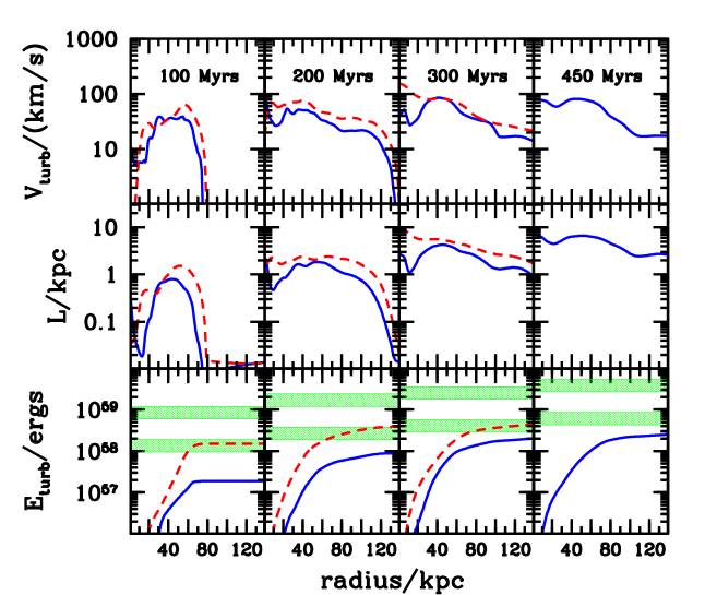
Figure 19.— Radial profile of turbulence quantities in the evacuated multiple bubble run (5DCER, solid lines), and the Sedov multiple-bubble run (5DCSR, dashed lines), at times of 100 Myrs, 200 Myrs, 300 Myrs, and 450 Myrs, arranged in columns from left to right. From top to bottom the rows show the average turbulent velocity and txurbulent length scale as a function of radius, and the total turbulent kinetic energy within this radius. As in Figure 14 the shaded regions in the lower panels show $1-2$ of $E_{\rm buoyancy}$ and $E_{\rm expand}+E_{\rm buoyancy}.$

Finally, in Figure 19 we compare the subgrid turbulence quantities between the evacuated repeated bubble run (5DCER) and the Sedov repeated bubble run (5NCER). As in the single bubble runs turbulent velocities are only slightly increased by the RM instability, even though the total energy input in this case is substantially higher. Thus $V_{\rm turb}\approx 100-200$ km/s in both runs, roughly $15-30\%$ of the sound speed of the cluster. Although this is somewhat smaller than the Mach number of $\approx 0.5$ suggested by the resonance line studies of Perseus by Churazov et al. (2005), again our model only provides a lower limit on this value as it does not include all mechanisms that drive turbulence.

Comparing the turbulent length scale between the two runs, we again find that the enhancement in the Sedov bubble case is not dramatic. Apart from a noticeable increase in $L$ at $R\mathrel{\hbox{\hbox to0.0pt{\hbox{\lower 4.0pt\hbox{$\sim$}}\hss}\hbox{$<$}}}20$ kpc in the Sedov bubble runs, both runs achieve similar values of $L$, which averages $\approx 5$ kpc. Combining $L$ and $V$ to construct a diffusion coefficient gives typical values of $500$ kpc km/s, which are in excellent agreement with the effective diffusion coefficient inferred by the abundance profiles studies of Perseus by Rebusco et al. (2005), again suggesting that more complete self-regulating models with subgrid turbulence could do well at explaining this and other clusters.

In all cases, the total turbulent energy, shown in the the bottom panels, is $\approx$ 1-2% of the buoyant energy in the bubbles, and even a smaller fraction of $E_{\rm buoyancy}+E_{\rm expand}.$ Thus, as suggested above, turbulent dissipation is not likely to be an important factor. Rather it is the turbulent mixing of heated and enriched gas that plays a fundamental role in the evolution of AGN-heated galaxy clusters.

6. Conclusions

A wide range of observations suggest that AGN-feedback plays a key role in the evolution of cool-core galaxy clusters. At the same time, theoretical studies have pointed out some of the many physical mechanisms that may be important in this evolution, including viscosity, magnetohydrodynamic effects, heat conduction, and cosmic-ray heating. While any or all of these may operate in nature, none of them can be fully understood without first accurately capturing the underlying hydrodynamic evolution of the ICM. It is with this basic goal in mind that we have used a subgrid turbulence model to study AGN heating in an inviscid fluid, neglecting other effects such as magnetic fields and heat-conduction.

Within this context, our study has been focused on two key issues: the growth of instabilities and turbulence caused by AGN-heated bubbles and the role of these instabilities in determining the evolution of the bubbles and the surrounding medium. Clearly, there are other sources of turbulence that might add similar levels of turbulent energy into the ICM, such as mergers of large subclusters or motions of galaxies within a cluster. Likewise, the DT06 subgrid turbulence model that we have employed does not include all processes that generate turbulence, such as the shear-driven Kelvin-Helmholtz instability. However, our tests show that it is effective in capturing the growth of the extremely important RT and RM instabilities. Thus although many aspects of cluster evolution remain uncertain and beyond the scope of this work, there are a number of robust conclusions that we can make about the role of these two instabilities in shaping the evolution and impact of AGN-heated cavities in clusters. In particular we find that:

• Many of the RT and RM unstable modes that drive the evolution of the bubbles evolve on scales that are far below the resolution limits of current simulations. The superposition of these unstable modes smears out the interface between the bubbles and the ambient medium, transforming them into clouds of mixed material that stay intact and expand as they rise in the stratified cluster medium. This mixing can explain the coherent X-ray cavities detected in clusters of galaxies. The subgrid-turbulence model also greatly reduces the sensitivity of our results on the resolution of the computational grid and the detailed choice of initial conditions.

• Within the clouds, turbulent motions quickly attain typical velocities of $\approx 200$ km s${}^{-1},$ roughly $10\%$ of the internal sound speed and $20\%$ of the sound speed of the surrounding ICM. Similarly, the scale of the turbulent eddies rises swiftly but does not exceed the $\approx 30$ kpc scale of clouds. A typical turbulent diffusivity is then $\approx 500$ km/s kpc, which is in excellent agreement with the diffusion coefficient inferred by the abundance profiles studies of Perseus by Rebusco et al. (2005).

• Subgrid turbulence is likely to enhance metal transport significantly. In our fiducial single-bubble evacuated pure-hydro run, metal transport is halted at $\approx 50$ kpc by bubble disruption, which occurs when RT instabilities have shredded the evacuated region into resolution-limited cavities. Yet, in the subgrid-turbulence run, small-scale fluctuations act to keep the cloud coherent for much longer, thus causing it to distribute metals out to larger radii.

• In the case where the bubbles produce shock waves, the turbulent velocities and length scales are systematically enhanced with respect to the evacuated-bubble run, due to the RM instability. While such $\approx 300$ km/s velocities are roughly 50% greater than in the runs with evacuated bubbles, they are still well below the $\approx 500$ km/s radial velocities of the clouds. However they are large enough to be probed by studying the emission lines of heavy ions with the future Constellation-X satellite, which will have an envisaged spectral resolution of 1-2 eV.

• Calculating the turbulent kinetic energy produced by the rising bubbles, we find that this is only $\approx 1\%$ of the total energy available for the bubbles to heat the cluster. Hence, we do not expect the energy of the turbulent motions themselves to play a major role in the heating of the cool-core regions of the ICM. Rather, the main role of turbulence is to increase the efficiency with which the thermal energy of the rising clouds is mixed into the surrounding gas.

• Finally, runs that include radiative cooling and multiple episodes of AGN-feedback indicate that the impact of turbulence continues to increase with successive generations of heating. This is because turbulence driven by previous feedback events remains behind, enhancing the mixing of subsequent bubbles. While in our pure-hydro runs, the bubbles deposit most of their internal energy at the resolution-dependent radius at which they are disrupted, the turbulent motions captured by the subgrid model lead to more gradual heating, correspondingly shallower temperature and entropy profiles, and shallower metal gradients.

In summary, the properties, evolution, and appearance of AGN-blown bubbles in clusters are substantially different when one properly accounts for turbulent motions on scales well below the limits of current pure-hydro simulations. Although accounting for these motions may not provide the ultimate solution to many of the mysteries surrounding galaxy clusters, it is a crucial step forward in the modeling of feedback and the interaction between AGN and the ICM. Subgrid models such as the one developed in DT06 provide us with tools for capturing this physics. In fact, the numerical methodology presented here is likely to have applications in other areas of astrophysics where hydrodynamic modeling of RT instabilities is crucial, such as supernovae, supernova remnants, and galactic winds. It is clear that while many physical processes may play important roles in clusters and other environments, these can only be understood when carefully disentangled from the impact of subgrid turbulence.

References

- (1) Allen, S. W., & Fabian, A. C. 1998, MNRAS, 297, L63
- (2) Alon, U., Hecht, J., Ofer, D., & Shvarts, D. 1995, Phs. Rev. Lett. 74, 534
- (3) Balbus, S. A., Hawley, J. F., & Stone, J. M. 1996, ApJ, 467, 76
- (4) Bîrzan, L., Rafferty, D. A., McNamara, B. R., Wise, M. W., & Nulsen, P. E. J. 2004, ApJ, 607, 800
- (5) Blandford, R.D., & Rees, M. J. 1974, MNRAS, 169, 395
- (6) Blanton, E. L., Sarazin, C. L., McNamara, B. R., & Wise, M. W. 2001, ApJ, 558, L15
- (7) Boehringer, H., Voges, W., Fabian, A.C., Edge, A.C., & Neumann, D.M. 1993, MNRAS 264, L25
- (8) Bregman, J. N., & David, L. P. 1989, ApJ, 341, 49
- (9) Brighenti, F., & Mathews, W. G. 2006, ApJ, 643, 120
- (10) Brüggen, M., & Kaiser, C. R. 2001, MNRAS, 325, 676
- (11) Brüggen, M., & Kaiser, C. R. 2002, Nature, 418, 301
- (12) Brüggen, M., Ruszkowski, M., & Hallman, E. 2005a, ApJ, 630, 740
- (13) Brüggen, M., Hoeft, M., & Ruszkowski, M. 2005b, ApJ, 628, 153
- (14) Brunetti, G., & Lazarian, A. 2007, MNRAS, 378, 245
- (15) Carilli, C. L., Perley, R.A., & Harris, D. E. 1994, MNRAS 270, 173
- (16) Carilli, C. L., & Taylor G. B. 2002, ARA&A, 40, 319
- (17) Chandran, B.D.G. 2005, ApJ, 632, 809
- (18) Chandrasekhar S., 1961, Hydrodynamic and Hydromagnetic Stability. Dover
- (19) Chen, Y., Glimm, D. A., Sharp, D. A., & Zhang, Q. 1996, Phys. Fluids, 8, 816
- (20) Choi, Y. Y., Reynolds, C. S., Heinz, S., Rosenberg, J. L. Perlman, E. S., & Yang, J. 2004, ApJ, 606, 185
- (21) Churazov, E., Forman W., Jones C., & Böhringer, H. 2003, ApJ, 590, 225
- (22) Churazov, E., Forman, W., Jones, C., Sunyaev, R., & Böhringer, H. 2004, MNRAS, 347, 29
- (23) Colella, P., & Woodard, P. 1984, Jour. Comp. Phys, 52, 174
- (24) Colella, P., & Glaz, H. M. 1985, Jour. Comp. Phys, 52, 174
- (25) David, L. P., & Nulsen, P. E. J. 2008, ApJ, submitted (arXiv:0802.1165)
- (26) De Grandi, S., Ettori S., Longhetti M., & Molendi S. 2004, A&A, 419, 7
- (27) De Young, D. S. 2003, MNRAS, 343, 719
- (28) De Grandi, S., & Molendi, S. 2001, ApJ, 551, 153
- (29) De Grandi, S., & Molendi, S. 2002, ApJ, 567, 163
- (30) Dimonte, G. 1999, Phys. Plasmas. 6, 2009
- (31) Dimonte, G., & Tipton, G. 2006, Phys. of Fluids, 18 085101
- (32) Fabian, A. C. 1994, ARA&A, 32, 277
- (33) Fabian, A. C., et al. 2003, MNRAS, 344,43
- (34) Fabian, A. C., Sanders, J.S., Taylor, G.B., Allen, S.W., Crawford, C.S., Johnstone, R.M., & Iwasawa, K. 2006, MNRAS, 366, 417
- (35) Finoguenov, A., & Jones, C. 2001, ApJ, 547, L107
- (36) Fryxell, B. A., Müller, E., & Arnett, D. 1989, in Numerical Methods Astrophys, ed. P.R. Woodward (New York: Academic)
- (37) Fryxell B., et al. 2000, ApJS, 131, 273
- (38) Fukazawa, Y., et al. 2000, MNRAS, 313, 21
- (39) Glasstone, S., & Dolan, P. J. 1977, The Effects of Nuclear Weapons, 3rd edn. Washington, DC: United States Department of Defense and Energy Research and Development Administration
- (40) Glimm, J., Grove, J. W., Li, X. L., Oh, W., & Sharp, D. H. 2001, J. Comput. Phys., 169, 652
- (41) Godunov, S K. 1959, Mat. Sbornik, 47, 271
- (42) Holmes, R., et al. 1999, 389, 55
- (43) Iapichino, L., & Niemeyer, J. C. 2008, MNRAS, submitted (arXiv0801.4729)
- (44) Inogamov, N. A., & Sunyaev, R. A. 2003, Ast. Lett., 29, 791
- (45) Kelvin, W. T. 1871, Philosophical Magazine, 42, 362
- (46) Kim, W.-T. 2007, ApJ, 667, L5
- (47) Kraft, R.P., et al. 2003, ApJ, 592, 129
- (48) Llor, A. 2003, Laser Part. Beams, 21, 305
- (49) Loken, C., Roettiger, K., Burns, J. O., & Norman, M. 1995, ApJ, 445, 80
- (50) Matsushita K., Belsole E., Finoguenov A., & Böhringer, H. 2002, A&A, 386, 77
- (51) McNamara, B. R., et al. 2000 534, L135
- (52) McNamara, B. R., et al. 2001, ApJ, 562, L149
- (53) McNamara, B. R., et al. 2005, Nature, 433, 45
- (54) McNamara, B. R., et al. 2007, ARA&A, 45, 117
- (55) Meshkov, E. E. 1969, Izv. Akad. Nauk SSSR, Meckh. Zhid. Gaza, 4, 151
- (56) Mikaelian, K. 1989, Physica D. 36, 343
- (57) Narayan, R., & Medvedev, M.V. 2001, ApJL, 562, 129
- (58) Norman, M., & Bryan, G. 1999, in The Radio Galaxy Messier 87, ed. H.-J. Röser & K. Meisenheimer (Berlin: Springer), 106
- (59) Nulsen, P.E.J., McNamara, B. R., Jones, C., Forman, W. R., & Wise, M. 2002, ApJ, 568, 163
- (60) Nulsen, P.E.J., McNamara, B.R., Wise, M.W., & David, L.P. 2005, ApJ, 628, 629
- (61) Nulsen, P.E.J., et al. 2006, preprint (astro-ph/0611136)
- (62) Peres, G., Serio, S., Vaiana, G. S., & Rosner, R. 1982, ApJ 252, 791
- (63) Pizzolato, F., & Soker, N. 2006, MNRAS, 371, 1835
- (64) Porter, D. H., & Woodward, P. R. 1994, ApJS, 93, 309
- (65) Ramshaw, J.D. 1998, Phys, Rev. E, 58, 5834
- (66) Raymond, J. C., Cox, D. P. Cox, & Smith, B. W. 1976, ApJ. 204, 290
- (67) Rebusco P., Churazov, E., Böhringer H., & Forman W., 2005, MNRAS, 359, 1041
- (68) Rebusco, P., Churazov, E., Böhringer, H., & Forman, W. 2006, MNRAS, 372, 1840
- (69) Renzini A., Ciotti L., D’Ercole A., & Pellegrini S., 1993, ApJ, 419, 52
- (70) Reynolds C. S., Heinz, S., & Begelman, M. C. 2002, MNRAS, 332, 271
- (71) Reynolds C. S., McKernan, B., Fabian, A. C., Stone, J. M., & Vernaleo, J.C., 2005, MNRAS, 357, 242
- (72) Reynolds, C. S., Casper, E. A., & Heinz, S. 2008, ApJ, in press (arXiv:0802.0499)
- (73) Richtmyer, R. D. 1960, Pure Appl. Math. 13, 297
- (74) Ricker, P. M., & Sarazin, C. L. 2001, ApJ, 561, 621
- (75) Robinson, K., et al. 2004, ApJ, 601, 621
- (76) Roediger, E., Brüggen, M., Rebusco, P. Böhringer, H., & Churazov, E. 2007, MNRAS, 375, 15 (R07)
- (77) Ruszkowski, M., Brüggen M., & Begelman, M. C. 2004, ApJ, 611, 158
- (78) Ruszkowski, M., Enßlin, T. A., Brüggen, M., Heinz, S., & Pfrommer, C. 2007, MNRAS, 378, 662
- (79) Sarazin, C. L. 1986, RvMP, 58, 1
- (80) Schmidt R. W., Fabian A. C., & Sanders J. S. 2002, MNRAS, 337, 71
- (81) Schuecker, P., Finoguenov, A., Miniati, F., Böhringer, H., & Briel, U. G. 2004, A&A, 426, 387
- (82) Simionescu, A., Böhringer, H., Brüggen, M., & Finoguenov, A. 2007, A&A, 465,749
- (83) Sijacki, D., & Springel, V. 2006, MNRAS, 371, 1025
- (84) Soker, N. 2004, NewA, 9, 285
- (85) Sternberg, A., Pizzolato, F., & Soker, N. 2007, ApJ, 656, L5
- (86) Sternberg, A., & Soker, N. 2008a, MNRAS, 384, 1327
- (87) Sternberg, A., & Soker, N. 2008b, MNRAS, in press (arXiv:0805.2275)
- (88) Sytine, I. V., Porter, D. H., Woodward, P. R., Hodson, S. W., & Winkler, K.-H. 2000, JCoPh, 158, 225
- (89) Takizawa, M. 2005, ApJ, 629, 791
- (90) Tamura, T., et al. 2001, A&AL, 365, 87
- (91) Vogt, C., & Ensslin, T. A. 2005, A&A, 434, 67
- (92) Voigt, L. M., & Fabian, A. C. 2004, MNRAS, 347, 1130
- (93) Voit, G. M, & Bryan, G. L. 2001, Nature, 414, 425
- (94) Voit, G. M., Cavagnolo, K. W., Donahue, M., Rafferty, D. A., McNamara, B. R., & Nulsen, P. E. J. 2008, ApJ, submitted
- (95) von Helmholtz, H. L. F. 1868, Monatsberichte der Königlichen Preussiche Akademie der Wissenschaften zu Berlin 23, 215
- (96) Woodward, P., & Colella, P. R. 1984, JCoPh, 54, 174
- (97) Youngs, D. L. 1989, Physica D, 37, 270