Implications of Two Type Ia Supernova Populations for Cosmological Measurements

Abstract

Recent work suggests that Type Ia supernovae (SNe) are composed of two distinct populations: prompt and delayed. By explicitly incorporating properties of host galaxies, it may be possible to target and eliminate systematic differences between these two putative populations. However, any resulting post-calibration shift in luminosity between the components will cause a redshift-dependent systematic shift in the Hubble diagram. Utilizing an existing sample of 192 SNe Ia, we find that the average luminosity difference between prompt and delayed SNe is constrained to be $(4.5\pm 8.9)\%$. If the absolute difference between the two populations is 0.025 mag, and this is ignored when fitting for cosmological parameters, then the dark energy equation of state (EOS) determined from a sample of 2300 SNe Ia is biased at $\sim 1\sigma$. By incorporating the possibility of a two-population systematic, this bias can be eliminated. However, assuming no prior on the strength of the two-population effect, the uncertainty in the best-fit EOS is increased by a factor of 2.5, when compared to the equivalent sample with no underlying two-population systematic. To avoid introducing a bias in the EOS parameters, or significantly degrading the measurement accuracy, it is necessary to control the post-calibration luminosity difference between prompt and delayed SN populations to better than 0.025 mag.

1. Introduction

The discovery of the accelerating expansion of the universe (Riess et al., 1998; Perlmutter et al., 1999) has led to an explosion of interest in the underlying physics responsible for this acceleration. A favored model characterizes the acceleration by an unknown energy density component, dubbed the dark energy. While there exist a variety of probes to explore the nature of this dark energy, one of the most compelling entails the use of type Ia supernovae (SNe henceforth) to map the expansion history of the universe. Several present and future SN surveys are aimed at constraining the dark energy equation-of-state (EOS) to better than 10%. With increasing sample sizes, SN distances can potentially provide multiple independent estimates of the EOS of dark energy when binned in redshift (Huterer & Cooray, 2005; Sullivan, Cooray, & Holz, 2007; Sarkar et al., 2008a). Given the importance of dark energy measurements, it is then useful to quantify various systematics that impact SN cosmology (Hui & Greene, 2006; Cooray & Caldwell, 2006; Cooray et al., 2006; Sarkar et al., 2008b).

Recently, suggestions have been made that the SN population consists of two components, with a “prompt” component proportional to the instantaneous host galaxy star formation rate, and a “delayed” (or “extended”) component that is delayed by several Gyrs (Hamuy et al., 1995; Livio, 2000; Scannapieco and Bildsten, 2005; Mannucci et al., 2006; Sullivan et al., 2006; Strovink, 2007). The former is expected to be more luminous, and thus, prompt SN lightcurves are broader than those of the delayed population. By classifying SNe by host galaxy type, Howell et al. (2007) found a pre-calibration intrinsic luminosity difference of $\sim(12\pm 4)$% between the two components, based on a difference of $(8.1\pm 2.7)\%$ in the width of lightcurves. Since the SN lightcurves are used to calibrate the intrinsic luminosity (Phillips, 1993; Riess et al., 1996; Perlmutter et al., 1997; Tonry et al., 2003; Prieto et al., 2006; Guy et al., 2007; Jha et al., 2007), a systematic difference in intrinsic luminosity could conceivably be calibrated out, if the SN lightcurve calibration relation is the same for both populations.

However, it is unclear whether the full intrinsic difference in luminosity between the two populations is captured by a calibratable difference in the lightcurves. A residual in the calibrated luminosity could potentially remain, leading to a redshift-dependent shift in the Hubble diagram, and systematic errors in the best-fit cosmological parameters. For example, it is likely that the intrinsic colors of Type Ia SNe are not uniquely determined by light-curve shape (Conley et al., 2008). Even if this is not the case, differences in intrinsic color between the populations might introduce systematic differences in post-calibration luminosity (e.g., through differences in the extinction corrections). We model the two-population systematic, constraining the magnitude of the effect with current data. With large SN samples it may be possible to estimate the magnitude of the systematic directly from the data (e.g., by correlating observed SN brightnesses with properties of the host galaxies (Hamuy et al., 1996b; Riess et al., 1999; Sullivan et al., 2006; Jha et al., 2007; Gallagher et al., 2008)). We quantify the level of calibration required to avoid significantly degrading the determination of the dark energy EOS.

The paper is organized as follows: in $\S$2 we discuss a model for incorporating a two-population systematic residual luminosity into the Hubble diagram. In $\S$3 we investigate the possibility of detecting this systematic from both current and future SN data, and the impact on dark energy parameter estimation.

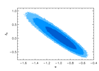
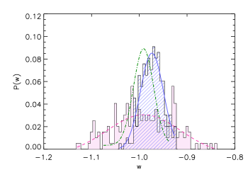
Figure 1.— Left panel: Correlation between $\delta_{D}$ and $w$, corresponding to a $w$CDM model, for the 192 SN dataset discussed in the text. There is a strong degeneracy between the two-population systematic, $\delta_{D}$, and the dark energy EOS, $w$. This leads to a potential bias in the measurement of the EOS, and increased errors when the fits are marginalized over $\delta_{D}$. Right panel: Histograms showing the distributions of the best-fit $w$, from 200 mock data sets with an inherent $\delta_{D}=0.025$, after marginalizing over the WMAP $w$CDM 5-Year priors. The shaded histogram represents the case where $\delta_{D}$ is allowed to vary freely, while for the hatched histogram the two-population systematic is ignored ($\delta_{D}=0$). The dot-dashed line corresponds to the case where the data is fit assuming a $\delta_{D}=0.025\pm 0.025$ prior. For clarity we omit the underlying histogram.

2. Two SN Populations and the Hubble Diagram

The use of SNe as standardizable candles to constrain the dark energy EOS is based on the fundamental assumption that the lightcurves of all individual SNe can be calibrated. The lightcurve shape-intrinsic luminosity relation is derived using low-$z$ samples of SNe, and it is assumed that this relation is applicable to the higher-$z$ population. However, if the SN population is non-uniform with redshift, the potential for systematics must be considered (Howell, 2001; Mannucci et al., 2006; Scannapieco and Bildsten, 2005; Sullivan et al., 2006).

According to the two-population model of Scannapieco and Bildsten (2005) (henceforth SB), the prompt SNe track the instantaneous star formation rate, $\dot{M_{*}}(t)$, and dominate the total SN rate at early times (high redshifts) when star formation is more active. The rate of the delayed component scales proportionally to the total stellar mass at a given instant, $M_{*}(t)$, and thus delayed SNe dominate at late times (low redshifts). The total SN rate can be written as

$$\frac{SNR_{\mbox{\footnotesize Ia}}(t)}{(100\,\mbox{yr})^{-1}}=A\left[\frac{M_{*}(t)}{10^{10}M_{\sun}}\right]+B\left[\frac{\dot{M_{*}}(t)}{10^{10}M_{\sun}\mbox{Gyr}^{-1}}\right]$$ (1)

where $A$ and $B$ are dimensionless constants. We take the star formation rate proportional to $e^{-t/(2Gyr)}$ (Mannucci et al., 2006). This model is likely to be a simple approximation to a true, smooth underlying distribution of delay times (Totani et al., 2008; Greggio et al., 2008; Pritchet et al., 2008). For simplicity we restrict ourselves to the two-population model, although in §3.2 we discuss sensitivity to this assumption.

We allow for a redshift-independent residual difference ($\Delta{L}$) in the calibrated absolute luminosities of the prompt (${L}_{P}$) and delayed (${L}_{D}$) SNe: $L_{P}=L_{D}+\Delta L$. We take the delayed and prompt fractions of the total SN population to be $f_{D}(z)$ and $f_{P}(z)$, respectively ($f_{D}(z)+f_{P}(z)=1$).

The average of the distance moduli of all the SNe in a given redshift bin can be written as

$$\langle(m-M)\rangle=5\log_{10}\left(\frac{d_{L}}{\mbox{Mpc}}\right)+25-\bigg{\langle}2.5\log_{10}\left(\frac{L}{{L}_{ref}}\right)\bigg{\rangle}\,,$$ (2)

where $L_{ref}$ is the reference luminosity corresponding to the reference absolute magnitude $M_{ref}$ given by $M_{ref}=\bar{f}_{D}M_{D}+\bar{f}_{P}M_{P}$, where $\bar{f}_{i}$ is the redshift-average of $f_{i}(z)$ over the low redshift range where the calibration is done. The residual systematic correction to $\langle(m-M)\rangle$ can be expressed as $\langle(m-M)\rangle_{\mbox{\scriptsize res}}=\delta_{D}f_{D}(z)-2.5\log_{10}({L}_{P}/{L}_{ref})$, where $\delta_{D}=1.086\ln(1+\Delta L/L_{D})$ is the two-population bias. Note that one can also express $\langle(m-M)\rangle_{\mbox{\scriptsize res}}$ relative to the prompt component, using $\delta_{P}$ instead of $\delta_{D}$, and $f_{P}$ instead of $f_{D}$. This involves an overall sign change, but the final results are unaltered.

Using the $\chi^{2}$-statistic, we fit the Hubble diagram with a modified form of the distance modulus which includes a possible residual:

$$(m-M)^{\rm fid}(z)=5\log_{10}\left(\frac{d_{L}(z)}{\mbox{Mpc}}\right)+25+\mathcal{M}+\delta_{D}f_{D}(z).$$ (3)

We have absorbed the redshift-independent term in $\langle(m-M)\rangle_{\mbox{\scriptsize res}}$ into the “nuisance parameter”, $\mathcal{M}$. Note that $H_{0}$ is incorporated into $d_{L}$ instead of $\mathcal{M}$. The redshift-dependent factor $f_{D}(z)$ can be determined based on our knowledge of the star-formation history, and $\delta_{D}$ must be estimated directly from the SN data. This residual systematic must now be marginalized over, and will affect cosmological parameter estimates.

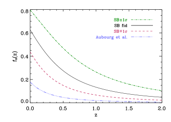
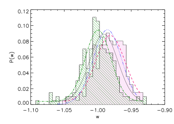
Figure 2.— Left panel: The fraction of the delayed component, $f_{D}$, as a function of redshift. The solid line corresponds to the fiducial $A$ and $B$ values from SB (Scannapieco and Bildsten, 2005) that are used to generate the mock catalogs. The dashed and dot-dashed lines correspond to $\{A-\Delta A,B+\Delta B\}$ and $\{A+\Delta A,B-\Delta B\}$, respectively, where $\Delta A$ and $\Delta B$ are the $1\sigma$ uncertainties on $A$ and $B$ from SB. The triple-dot-dashed line depicts the recent estimate of $f_{D}$ from Aubourg et al. (2007). Right panel: Histograms showing the best-fit values for the dark energy EOS parameter, $w$, for 200 mock SN datasets with $\delta_{D}=0.025$. The solid curve shows the Gaussian fit to $P(w)$ for the case where we use the same $f_{D}(z)$ to generate the mock catalogs and fit the data. The other Gaussian curves correspond to the best-fit values of $w$ when we fit the mock data with the wrong functional form for $f_{D}(z)$. The mocks are generated with the fiducial model, and the line-types represent the model used in the fit, in accordance with the left panel. For clarity we only show two underlying histograms, for the cases $\{A-\Delta A,B+\Delta B\}$ (shaded) and $\{A+\Delta A,B-\Delta B\}$ (hatched). A $\sim 30\%$ shift in $f_{D}$ (left panel) corresponds to a percent-level bias in $w$ (right panel). The extreme model of Aubourg et al. (2007) corresponds to an almost redshift-independent $f_{D}$ (see left panel), and thus the bias is similar to that in the $\delta_{D}=0$ case.

3. Residual systematic and parameter estimation

3.1. Existing data

To study the extent to which existing data may be affected by a residual systematic in the luminosity difference between prompt and delayed SNe, we model fit a combined data set of 192 SNe (Davis et al., 2007; Wood-Vasey et al., 2007; Riess et al., 2007; Astier et al., 2006; Hamuy et al., 1996a; Riess et al., 1999; Jha et al., 2006). We also include two baryon acoustic oscillation (BAO) distance estimates at $z=0.2$ and $z=0.35$ (Percival et al., 2007), and the dimensionless distance to the surface of last scattering $R=1.710\pm 0.019$ (Komatsu et al., 2008). We take a flat $\Lambda$CDM cosmological model and marginalize over $\mathcal{M}$, with WMAP priors of $H_{0}=71.9\pm 2.6$ and $\Omega_{m}h^{2}=0.1326\pm 0.0063$ (Komatsu et al., 2008). These priors are independent of the SN data. For simplicity we do not incorporate the correlation between $\Omega_{m}h^{2}$ and $H_{0}$. Such a correlation will not qualitatively alter our results, but will need to be taken into account once precision data becomes available.

The distribution function for $\delta_{D}$ from existing data has a positive mean value ($\delta_{D}=0.049$), implying that the post-calibration luminosity of the delayed population is dimmer than the prompt population by $\sim$5%. The standard deviation of this $\delta_{D}$ is $\sigma=0.097$, which suggests that current SN data is consistent with the absence of a two-population bias. The Howell et al. (2007) result of $\sim$ $(12\pm 4)$% difference in the intrinsic luminosity is a pre-calibration difference. We find a $\sim(5\pm 9)$% difference in the post-calibration luminosity between the two types of SNe. While this uncertainty is larger than the pre-calibration value, it is estimated directly from the Hubble diagram, and is independent of the empirical stretch-luminosity relation. This important consistency check will improve as the SN sample sizes increase.

To study the impact of a potential luminosity difference on the measurement of the dark energy EOS, we also fit the same data (SN+BAO+CMB) assuming a $w$CDM model, and take the corresponding WMAP+HST priors $H_{0}=72.1\pm 7.5$ and $\Omega_{m}h^{2}=0.1329\pm 0.0066$ (Komatsu et al., 2008; Freedman et al., 2001). We first consider two extreme cases: ignoring the two-population systematic ($\delta_{D}=0$), and allowing for a completely unconstrained systematic ($\delta_{D}$ with no priors). With $\delta_{D}$ free, our analysis yields a best-fit time-independent EOS parameter $w=-0.986\pm 0.180$, with a best-fit $\delta_{D}=0.040\pm 0.279$. If we set $\delta_{D}=0$, the same data provides a constraint of $w=-0.960\pm 0.066$. By incorporating a two-population effect in the fit, the errors on the best-fit EOS degrade by a factor of $\sim 3$. In addition, we note a shift in the best-fit value of $w$ between the two cases. The evolution in the ratio between prompt and delayed SNe, as a function of redshift, can mimic dark energy. If there is a residual difference in the calibrated luminosity, ignoring $\delta_{D}$ might bias the dark energy estimate. As we show in the left panel of Figure 1, the increase in the error of the best-fit EOS is due to the degeneracy between dark energy ($w$) and the two-population systematic ($\delta_{D}$).

Following Howell et al. (2007), it may be possible to calibrate out the luminosity difference between the two components with large samples of SNe (e.g., by looking for characteristic properties in the SN spectra, or by correlating SN luminosities with host galaxy types). This will lead to a prior constraint on $\delta_{D}$, although uncertainties will still remain on the redshift evolution (as estimated by $f_{D}(z)$). Assuming the two-population fraction, and its redshift evolution, is perfectly known, we analyze the same SN data assuming a Gaussian prior on $\delta_{D}$. Taking this prior to have zero mean and $\sigma=(0.25,0.1,0.05)$, the errors on $w$ are ($0.130,0.086,0.072$), with the best-fit value of $w$ being approximately the same as was found for the $\delta_{D}=0$ case. Thus, by including a two-population systematic in the fit, with a prior on $\delta_{D}$ centered at 0 with a 0.05 mag dispersion, we recover the same best-fit $w$, but with $\sim 10\%$ degradation in the error bars.

3.2. Future data

We now turn to proposed SN surveys, and investigate how uncertainties in a possible two-population systematic impact measurements of $w$. We generate mock SN catalogs with 300 SNe uniformly distributed at $z<0.1$, and 2000 SNe in the range $0.1\leq z\leq 1.7$, similar to a JDEM-like survey (Kim et al., 2004). We incorporate an intrinsic Gaussian scatter of 0.1 mag for each SN, and take the relative fraction of delayed and prompt SNe, $f_{D}(z)$, given by Eq. 1 with SB values of $A=4.4\times 10^{-2}$ and $B=2.6$. We assume different values (0.025, 0.05, 0.1 mag) for the underlying two-population bias ($\delta_{D}$).

We fit each mock data set of 2300 SNe, along with the 2 existing BAO measurements, to a $w$CDM model, with the corresponding $w$CDM WMAP+HST priors as before. When fitting the data we consider two extreme cases: $\delta_{D}=0$, and $\delta_{D}$ completely unconstrained. Our results for $\delta_{D}=0.025$, from 200 separate mocks, are summarized in the right panel of Figure 1. The hatched histogram, which peaks at -0.974, depicts the case where $\delta_{D}=0$ was assumed in the fit. This corresponds to a systematic being present in the data, but ignored in the fit. With an average error on the EOS of 0.029 from MCMC, the resulting bias in the best-fit EOS value is $\sim 1\sigma$ from the underlying value ($w=-1$).

The shaded histogram in the right panel of Figure 1, having a peak at -0.991 with a $1\sigma$ width of 0.071, shows the distribution of the best-fit $w$ with 200 mocks, where we let $\delta_{D}$ vary freely while fitting the data to Eq. 3. In this case we find no significant bias ($w=-1$ is recovered within $<0.1\sigma$), but the width of the distribution and MCMC results for each mock sample show that the errors in the best-fit $w$ increase by a factor of $\sim 2.5$. When the underlying two-population bias is $\delta_{D}=0.05$ mag, we find $w=-0.955\pm 0.030$ (assuming $\delta_{D}=0$ in the fit) and $w=-0.986\pm 0.067$ (assuming $\delta_{D}$ unconstrained) based on 50 Monte-Carlo realizations. Generating data with $\delta_{D}=0.1$, and neglecting the systematic in the fit, we find $w=-0.925\pm 0.029$ (50 realizations). As a rough rule, if the two-population systematic is neglected, the resulting bias in the best-fit $w$ is on the order of the magnitude of the underlying $\delta_{D}$.

Thus far we have assumed no prior knowledge on the values of $\delta_{D}$, although it may be possible to adduce a priori constraints on $\delta_{D}$ through SN population statistics combined with correlations to galaxy properties. We model-fit 200 separate SN mocks (with intrinsic $\delta_{D}=0.025$ mag) with two different priors: $\delta_{D}=0.025\pm 0.025$ and $\delta_{D}=0\pm 0.025$ mag. The former case represents knowledge of the true underlying systematic (with a $1\sigma$ uncertainty of 0.025 mag), while for the latter case the central value is incorrectly assumed to be zero (with a $0.025$ mag uncertainty). With the $\delta_{D}$ prior peaked on the correct value (0.025), the distribution of $w$ peaks at $-0.993$ with a $1\sigma$ width of 0.034 (the Gaussian with dot-dashed line in the right panel of Figure 1). With the prior centered on the wrong value (0 instead of 0.025), the distribution peaks at $w=-0.977$ (showing a small bias of $\sim 0.6\sigma$), with the same $1\sigma$ uncertainty of 0.034. In both cases the errors in $w$ increase by $\sim 30\%$, when compared to the equivalent dataset with no two-population effect in either the mock data or the fit.

Thus far we have assumed that we know $f_{D}(z)$ perfectly. Even if the two-population model is correct, uncertainties in $A$ and $B$, or equivalently uncertainties in the star-formation history, lead to a redshift-dependent uncertainty in $f_{D}(z)$. To test the effect of these uncertainties on parameter estimation, we generate mock data sets with $\delta_{D}=0.025$, and $f_{D}(z)$ taken to be the canonical two-parameter form given in Eq. 1. We then fit these data assuming different forms for $f_{D}(z)$ obtained by accounting for uncertainties in $A$ and $B$ from SB. We also consider an estimate of $f_{D}$ from Aubourg et al. (2007). The resulting $f_{D}$ curves are shown in the left panel of Figure 2. In the right panel we show the resulting bias in dark energy EOS measurements, as a result of the uncertainty in $f_{D}$. The uncertainties in the population fraction lead to biases in the resulting EOS parameters. To control this bias to the percent level, the underlying distribution must be characterized to $\lesssim 20\%$.

In summary, we have found that a post-calibration shift in the standard-candle brightness between delayed and prompt SNe can introduce bias in the best-fit dark energy parameters. By controlling the magnitude of any resulting two-population difference to better than 0.025 mag, the bias can be kept under 1$\sigma$ for a JDEM-like survey without significantly degrading the accuracy of the dark energy measurements.

References

- Astier et al. (2006) Astier, P. et al., 2006, A & A, 447, 31
- Aubourg et al. (2007) Aubourg, E. et al., 2007, arXiv.org:0707.1328
- Conley et al. (2008) Conley, A. et al., 2008, ApJ, 681, 482
- Cooray & Caldwell (2006) Cooray, A., & Caldwell, R. R. 2006, PRD, 73, 103002
- Cooray et al. (2006) Cooray, A., Huterer, D. & Holz, D. 2006, PRL, 96, 021301
- Davis et al. (2007) Davis, T. M., et al., 2007, ApJ, 666, 716
- Freedman et al. (2001) Freedman, W. L., et al., 2001, ApJ, 553, 47
- Gallagher et al. (2008) Gallagher, J. S. et al., 2008, arXiv:0805.4360
- Greggio et al. (2008) Greggio, L. et al., 2008, arXiv:0805.1512v2
- Guy et al. (2007) Guy, J., et al., 2007, A&A, 466, 11
- Hamuy et al. (1995) Hamuy, M., et al., 1995, AJ, 109, 1
- Hamuy et al. (1996a) Hamuy, M., et al., 1996a, AJ, 112, 2408
- Hamuy et al. (1996b) Hamuy, M., et al., 1996b, AJ, 112, 2438
- Howell (2001) Howell, D. A. 2001, ApJ, 554, L193
- Howell et al. (2007) Howell, D. A. , et al. 2007, ApJ, 667, L37
- Hui & Greene (2006) Hui, L. & Greene, P. B. 2006, PRD, 73, 123526
- Huterer & Cooray (2005) Huterer, D. & Cooray, A. 2005, PRD, 71, 023506
- Jha et al. (2006) Jha, S. et al. 2006, AJ, 131, 527
- Jha et al. (2007) Jha, S., Riess, A. G., and Kirshner, R. P., 2007, ApJ, 659, 122
- Kim et al. (2004) Kim, A. G., et al. 2004, MNRAS, 347, 909
- Komatsu et al. (2008) Komatsu, E., et al., 2008, arXiv:0803.0547
- Livio (2000) Livio, M. 2000, arXiv:astro-ph/0005344
- Mannucci et al. (2006) Mannucci, F., Della Valle, M., and Panagia, N., 2006, MNRAS, 370, 773
- Percival et al. (2007) Percival, W. J., et al. 2007, MNRAS, 381, 1053
- Perlmutter et al. (1997) Perlmutter, S., et al. 1997, ApJ, 483, 565
- Perlmutter et al. (1999) Perlmutter, S., et al. 1999, ApJ, 517, 565
- Phillips (1993) Phillips, M. M. 1993, ApJ, 413, L105
- Prieto et al. (2006) Prieto, J. L., Rest, A., and Suntzeff, N. B., 2006, ApJ, 647, 501
- Pritchet et al. (2008) Pritchet, C. J. et al., 2008, arXiv:0806.3729
- Riess et al. (1996) Riess, A. G., Press, W. H., and Kirshner, R. P. 1996, ApJ, 473, 88
- Riess et al. (1998) Riess, A. G. et al. 1998, AJ, 116, 1009
- Riess et al. (1999) Riess, A. G. et al. 1999, AJ, 117, 707
- Riess et al. (2007) Riess, A. G., et al. 2007, ApJ, 659, 98
- Sarkar et al. (2008a) Sarkar, D., et al. 2008a, PRL, 100, 241302 [arXiv:0709.1150]
- Sarkar et al. (2008b) Sarkar, D., et al. 2008b, ApJ, 678, 1 [arXiv:0710.4143]
- Scannapieco and Bildsten (2005) Scannapieco, E. and Bildsten, L. 2005, ApJ, 629, L85
- Strovink (2007) Strovink, M. 2007, ApJ, 671, 1084
- Sullivan et al. (2006) Sullivan, M., et al. 2006, ApJ, 648, 868
- Sullivan, Cooray, & Holz (2007) Sullivan, S., Cooray, A., & Holz, D. E. 2007, JCAP, 09, 004
- Totani et al. (2008) Totani, T. et al., 2008, arXiv:0804.0909
- Tonry et al. (2003) Tonry, J. L. et al. 2003, ApJ, 594, 1
- Wood-Vasey et al. (2007) Wood-Vasey, W. M., et al. 2007, ApJ, 666, 694