Light-pulse atom interferometry

Abstract

The light-pulse atom interferometry method is reviewed. Applications of the method to inertial navigation and tests of the Equivalence Principle are discussed.

1 Introduction

De Broglie wave interferometry using cold atoms is emerging as a new tool for basic science and technology. There are numerous approaches and applications which have evolved since the first demonstration experiments in the early 1990’s. These notes will not attempt an exhaustive or comprehensive survey of the field. An excellent overview is provided in Ref. [1] and other lectures in this volume. These notes will focus on what has become known as light-pulse atom interferometry, which has found fruitful applications in gravitational physics and inertial sensor development.

These notes are organized as follows. We we first summarize basic theoretical concepts. We will then illustrate this formalism with a discussion of applications in inertial navigation and in a detailed design discussion of an experiment currently under development to test the Weak Equivalence Principle.

2 Atom interferometry overview

By analogy with their optical counterparts, atom interferometery seeks to exploit wave interference as a tool for precision metrology. In this measurement paradigm, a single particle (photon or atom) is made to coherently propagate over two paths. These paths are subsequently recombined using a beamsplitter, and their relative phase becomes manifest in the probability of detecting the particle in a given output port of the device. Hence, measuring the particle flux at the interferometer output ports enables determination of the phase shift. As this relative phase depends on physical interactions over the propagation paths, this enables the characterization of these interactions.

A key challenge for de Broglie wave interferometers is the development of techniques to coherently divide and recombine atomic wavepackets. For simplicity, consider an atom with initial momentum $\mathbf{p}$, characterized by a wavefunction $\psi(\mathbf{x})\sim\exp{\left[\frac{i}{\hbar}{\bf p\cdot x}\right]}$ . The atom then is subject to a Hamiltonian interaction which is engineered to evolve the wavepacket into a momentum superposition state. One such interaction spatially modulates the amplitude of the wavefunction, so that, for example, $\exp{\left[\frac{i}{\hbar}{\bf p\cdot x}\right]}\rightarrow f(\mathbf{x})\exp{\left[\frac{i}{\hbar}{\bf p\cdot x}\right]}$, where $f(\mathbf{x})$ is a real periodic function with spatial frequency $\mathbf{k}$. Fourier decomposing $f(\mathbf{x})$ immediately shows that the final wavefunction is a coherent superposition of momenta $\mathbf{p}$, ${\bf p}\pm\hbar{\bf k}$, ${\bf p}\pm 2\hbar{\bf k}$, etc. In practice, such an interaction can be implemented by passing a collimated atomic beam through a microfabricated transmission grating, as demonstrated by Pritchard and co-workers [2].

Another interaction is one which spatially modulates the phase of the wavefunction. Consider, for example, $\psi(\mathbf{x})\rightarrow\exp{\left[i{\bf k\cdot x}\right]}\psi(\mathbf{x})$. This interaction results in a momentum translation ${\bf p}\rightarrow{\bf p}+\hbar{\bf k}$. A particularly useful implementation of this process imparts a spatial phase modulation by driving transitions between internal atomic states. For simplicity, consider a two-level atom with internal states $\left|1\right>$ and $\left|2\right>$ that are resonantly coupled by an applied optical traveling wave $\mathbf{E}\propto\exp{\left[i{\bf k}\cdot{\bf x}\right]}$ via the electric-dipole interaction $\hat{\mathbf{\mu}}\cdot\mathbf{E}$ (where $\hat{\mathbf{\mu}}$ is the dipole moment operator). If the atom is initially prepared in state $\psi(\mathbf{x})\left|1\right>$, then following an interaction time $t$ its state becomes $\alpha(t)\psi(\mathbf{x})\left|1\right>$ + $\beta(t)\exp{\left[i{\bf k}\cdot{\bf x}\right]}\psi(\mathbf{x})\left|2\right>$ (see Section 3 for details). The interaction time can be chosen, for example, so that $|\alpha|$ = $|\beta|$ = $1/\sqrt{2}$ to implement a beamsplitter (the $\pi/2$ pulse condition). In this case, the internal state of the atom becomes correlated with its external momentum. In practice, two-photon stimulated Raman transitions between groundstate hyperfine levels have proven to be particularly fruitful for implementing this class of beamsplitter. Why? Transitions are made between long lived hyperfine levels while the phase grating periodicity is twice that of a single photon optical transition (when the Raman transition is driven in a counter-propagating beam geometry).

The above mechanisms operate in free space. A new family of atom optics, based on control of atom wavepacket motion in atomic waveguides, is under development. The basic idea is that atoms are steered using microfabricated wires deposited on surfaces. These are loosely analogous to optical fiber waveguides for light. In principle, coherent beamsplitters are implemented by the appropriate joining of waveguides. Recently, a combination of microwave and magnetic fields has allowed for creation of waveguide structures capable of coherent wavefront division. These structures have been used to demonstrate proof-of-principle interferometer topologies which have been used to study the coherence properties of the division process. The notes below will discuss free space atom optics, which have proven effective for precision measurement of inertial forces.

Exploiting the momentum exchange principles outlined above, it becomes straightforward to devise a de Broglie wave interferometer which is based on sequences of light pulses. For example, consider a three pulse sequence based on Raman transitions. An initial Raman $\pi/2$ pulse places an atom in a coherent superposition of wavepackets in states $\left|1\right>$ and $\left|2\right>$ whose mean momenta differ by $\hbar\mathbf{k}_{\text{eff}}$ (here $\mathbf{k}_{\text{eff}}$ is the effective wavevector of the Raman process, see below). After an interrogation time $T$ these wavepackets separate by a distance $\hbar k_{\text{eff}}T/m$, where $m$ is the atomic mass. A subsequent optical pulse is then applied whose duration is chosen to drive the transitions $\left|1\right>\rightarrow\left|2\right>$ and $\left|2\right>\rightarrow\left|1\right>$ with unit probability (a $\pi$ pulse). This pulse has the effect of redirecting the momenta of the wavepackets so that at a time $T$ later the wavepackets again overlap. A final $\pi/2$ pulse then serves as the exit beamsplitter.

3 Phase shift determination

In this section we review the method for calculating the phase difference between the two halves of the atom at the end of the light-pulse atom interferometer pulse sequence outlined above. These results are well-known [3, 4], but we are not aware of a complete, formal derivation of these rules in the literature. Other equivalent formalisms for this calculation do exist (see, for example [5, 6]). For Section 5.2 it is necessary to understand the formulae for the phase difference (Section 3.1). The proof of these formulae as well as a discussion of their range of validity is given in Section 3.2 but is not necessary for the rest of the paper.

3.1 Phase shift formulae

The main result we will show is that the total phase difference $\Delta\phi_{\text{tot}}$ between the two paths of an atom interferometer may be written as the sum of three easily calculated components:

$$\Delta\phi_{\text{tot}}=\Delta\phi_{\text{propagation}}+\Delta\phi_{\text{separation}}+\Delta\phi_{\text{laser}}.$$ (1)

For this calculation we take $\hbar=c=1$.

The propagation phase $\Delta\phi_{\text{propagation}}$ arises from the free–fall evolution of the atom between light pulses and is given by

$$\Delta\phi_{\text{propagation}}=\sum_{\text{upper}}\left(\int_{t\!_{I}}^{t\!_{F}}\!(L_{c}-E_{i})dt\right)-\sum_{\text{lower}}\left(\int_{t\!_{I}}^{t\!_{F}}\!(L_{c}-E_{i})dt\right)$$ (2)

where the sums are over all the path segments of the upper and lower arms of the interferometer, and $L_{c}$ is the classical Lagrangian evaluated along the classical trajectory of each path segment. In addition to the classical action, Eq. (2) includes a contribution from the internal atomic energy level $E_{i}$. The initial and final times $t_{I}$ and $t_{F}$ for each path segment, as well as $L_{c}$ and $E_{i}$, all depend on the path segment.

The laser phase $\Delta\phi_{\text{laser}}$ comes from the interaction of the atom with the laser field used to manipulate the wavefunction at each of the beamsplitters and mirrors in the interferometer. At each interaction point, the component of the state that changes momentum due to the light acquires the phase of the laser $\phi_{L}(t_{0},\mathbf{x}_{c}(t_{0}))=\mathbf{k}\cdot\mathbf{x}_{c}(t_{0})-\omega t_{0}+\phi$ evaluated at the classical point of the interaction:

$$\Delta\phi_{\text{laser}}=\left(\sum_{j}\pm\phi_{L}(t_{j},\mathbf{x}_{u}(t_{j}))\right)_{\text{upper}}-\left(\sum_{j}\pm\phi_{L}(t_{j},\mathbf{x}_{l}(t_{j}))\right)_{\text{lower}}$$ (3)

The sums are over all the interaction points at the times $t_{j}$, and $\mathbf{x}_{u}(t)$ and $\mathbf{x}_{l}(t)$ are the classical trajectories of the upper and lower arm of the interferometer, respectively. The sign of each term depends on whether the atom gains $(+)$ or loses $(-)$ momentum as a result of the interaction.

The separation phase $\Delta\phi_{\text{separation}}$ arises when the classical trajectories of the two arms of the interferometer do not exactly intersect at the final beamsplitter (see Fig. 1). For a separation between the upper and lower arms of $\mathbf{\Delta x}=\mathbf{x}_{l}-\mathbf{x}_{u}$, the resulting phase shift is

$$\Delta\phi_{\text{separation}}=\mathbf{\bar{p}}\cdot\mathbf{\Delta x}$$ (4)

where $\mathbf{\bar{p}}$ is the average classical canonical momentum of the atom after the final beamsplitter.

3.2 Justification of phase shift formulae

The interferometer calculation amounts to solving the Schrodinger equation with the following Hamiltonian:

$$\hat{H}_{\text{tot}}=\hat{H}_{\text{a}}+\hat{H}_{\text{ext}}+\hat{V}_{\text{int}}(\hat{\mathbf{x}})$$ (5)

Here $\hat{H}_{\text{a}}$ is the internal atomic structure Hamiltonian, $\hat{H}_{\text{ext}}$ is the Hamiltonian for the atom’s external degrees of freedom (center of mass position and momentum), and $\hat{V}_{\text{int}}(\hat{\mathbf{x}})=-\hat{\mathbf{\mu}}\cdot\mathbf{E}(\hat{\mathbf{x}})$ is the atom-light interaction, which we take to be the electric dipole Hamiltonian with $\hat{\mathbf{\mu}}$ the dipole moment operator.

The calculation is naturally divided into a series of light pulses during which $\hat{V}_{\text{int}}\neq 0$, and the segments between light pulses during which $\hat{V}_{\text{int}}=0$ and the atom is in free-fall. When the light is off, the atom’s internal and external degrees of freedom are decoupled. The internal eigenstates satisfy

$$i\partial_{t}\left|A_{i}\right>=\hat{H}_{\text{a}}\left|A_{i}\right>=E_{i}\left|A_{i}\right>$$ (6)

and we write the solution as $\left|A_{i}\right>=\left|i\right>e^{-iE_{i}(t-t_{0})}$ with time-independent eigenstate $\left|i\right>$ and energy level $E_{i}$.

For the external state solution $\left|\psi\right>$, we initially consider $\hat{H}_{\text{ext}}=H(\hat{\mathbf{x}},\hat{\mathbf{p}})$ to be an arbitrary function of the external position and momentum operators:

$$i\partial_{t}\left|\psi\right>=H(\hat{\mathbf{x}},\hat{\mathbf{p}})\left|\psi\right>.$$ (7)

It is now useful to introduce a Galilean transformation operator

$$\hat{G}_{c}\equiv\hat{G}(\mathbf{x}_{c},\mathbf{p}_{c},L_{c})=e^{i\int\!L_{c}dt}e^{-i\hat{\mathbf{p}}\cdot\mathbf{x}_{c}}e^{i\mathbf{p}_{c}\cdot\hat{\mathbf{x}}}$$ (8)

which consists of momentum boost by $\mathbf{p}_{c}$, a position translation by $\mathbf{x}_{c}$, and a phase shift. We choose to write

$$\left|\psi\right>=\hat{G}_{c}\left|\phi_{CM}\right>.$$ (9)

We will show that for a large class of relevant Hamiltonians, if $\mathbf{x}_{c}$, $\mathbf{p}_{c}$, and $L_{c}$ are taken to be the classical position, momentum and Lagrangian, respectively, then $\left|\phi_{CM}\right>$ is a wavepacket with $\left<\hat{\mathbf{x}}\right>=\left<\hat{\mathbf{p}}\right>=0$, and the dynamics of $\left|\phi_{CM}\right>$ do not affect the phase shift result (i.e., $\left|\phi_{CM}\right>$ is the center of mass frame wavefunction). However, for now we maintain generality and just treat $\mathbf{x}_{c}$, $\mathbf{p}_{c}$, and $L_{c}$ as arbitrary functions of time. Combining (7) and (9) results in

$$i\partial_{t}\left|\phi_{CM}\right> = \left\{\hat{G}_{c}^{\dagger}H(\hat{\mathbf{x}},\hat{\mathbf{p}})\hat{G}_{c}-i\hat{G}_{c}^{\dagger}\partial_{t}\hat{G}_{c}\right\}\left|\phi_{CM}\right>$$

$$= \left\{H(\hat{\mathbf{x}}+\mathbf{x}_{c},\hat{\mathbf{p}}+\mathbf{p}_{c})+\mathbf{\dot{p}}_{c}\cdot\hat{\mathbf{x}}-\left(\hat{\mathbf{p}}+\mathbf{p}_{c}\right)\cdot\mathbf{\dot{x}}_{c}+L_{c}\right\}\left|\phi_{CM}\right>$$

where we used the following identities:

$$\hat{G}_{c}^{\dagger}\hat{\mathbf{x}}\hat{G}_{c} = \hat{\mathbf{x}}+\mathbf{x}_{c}$$ (11)

$$\hat{G}_{c}^{\dagger}\hat{\mathbf{p}}\hat{G}_{c} = \hat{\mathbf{p}}+\mathbf{p}_{c}$$

$$\hat{G}_{c}^{\dagger}H(\hat{\mathbf{x}},\hat{\mathbf{p}})\hat{G}_{c} = H(\hat{\mathbf{x}}+\mathbf{x}_{c},\hat{\mathbf{p}}+\mathbf{p}_{c})$$

Next, we Taylor expand $H(\hat{\mathbf{x}}+\mathbf{x}_{c},\hat{\mathbf{p}}+\mathbf{p}_{c})$ about $\mathbf{x}_{c}$ and $\mathbf{p}_{c}$,

$$H(\hat{\mathbf{x}}+\mathbf{x}_{c},\hat{\mathbf{p}}+\mathbf{p}_{c})=H(\mathbf{x}_{c},\mathbf{p}_{c})+\nabla\!_{\hat{\mathbf{x}}}H(\mathbf{x}_{c},\mathbf{p}_{c})\cdot\hat{\mathbf{x}}+\nabla\!_{\hat{\mathbf{p}}}H(\mathbf{x}_{c},\mathbf{p}_{c})\cdot\hat{\mathbf{p}}+\hat{H}_{2}$$ (12)

where $\hat{H}_{2}$ contains all terms that are second order or higher in $\hat{\mathbf{x}}$ and $\hat{\mathbf{p}}$. (We will ultimately be allowed to neglect $\hat{H}_{2}$ in this calculation.) Inserting this expansion and grouping terms yields

$$i\partial_{t}\left|\phi_{CM}\right>=\left\{\big{(}H_{c}-\mathbf{\dot{x}}_{c}\cdot\mathbf{p}_{c}+L_{c}\big{)}+\big{(}\nabla\!_{\mathbf{x}_{c}}H_{c}+\mathbf{\dot{p}}_{c}\big{)}\cdot\hat{\mathbf{x}}+\big{(}\nabla\!_{\mathbf{p}_{c}}H_{c}-\mathbf{\dot{x}}_{c}\big{)}\cdot\hat{\mathbf{p}}+\hat{H}_{2}\right\}\left|\phi_{CM}\right>$$

where we have defined the classical Hamiltonian $H_{c}\equiv H(\mathbf{x}_{c},\mathbf{p}_{c})$. If we now let $\mathbf{x}_{c}$, $\mathbf{p}_{c}$, and $L_{c}$ satisfy Hamilton’s equations,

$$\mathbf{\dot{x}}_{c} = \nabla\!_{\mathbf{p}_{c}}H_{c}$$ (13)

$$\mathbf{\dot{p}}_{c} = -\nabla\!_{\mathbf{x}_{c}}H_{c}$$

$$L_{c} = \mathbf{\dot{x}}_{c}\cdot\mathbf{p}_{c}-H_{c}$$

with $\mathbf{p}_{c}\equiv\nabla\!_{\mathbf{\dot{x}}_{c}}L_{c}$ the classical canonical momentum, then $\left|\phi_{CM}\right>$ must satisfy

$$i\partial_{t}\left|\phi_{CM}\right>=\hat{H}_{2}\left|\phi_{CM}\right>$$ (14)

Next we show that it is possible to choose $\left|\phi_{CM}\right>$ with $\left<\hat{x}\right>=\left<\hat{p}\right>=0$ for a certain class of $\hat{H}_{2}$, so that $\mathbf{x}_{c}$ and $\mathbf{p}_{c}$ completely describe the atom’s classical center of mass trajectory. This is known as the semi-classical limit. Starting from Ehrenfest’s theorem for the expectation values of $\left|\phi_{CM}\right>$,

$$\partial_{t}\left<\hat{x}_{i}\right> = i\left<\left[\hat{H}_{2},\hat{x}_{i}\right]\right>=\left<\partial_{\hat{p}_{i}}\hat{H}_{2}\right>$$ (15)

$$\partial_{t}\left<\hat{p}_{i}\right> = i\left<\left[\hat{H}_{2},\hat{p}_{i}\right]\right>=-\left<\partial_{\hat{x}_{i}}\hat{H}_{2}\right>$$ (16)

and expanding about $\left<\hat{\mathbf{x}}\right>$ and $\left<\hat{\mathbf{p}}\right>$,

$$\partial_{t}\left<\hat{x}_{i}\right> = \left<\left.\partial_{\hat{p}_{i}}\hat{H}_{2}\right|_{\left<\hat{\mathbf{x}}\right>,\left<\hat{\mathbf{p}}\right>}+\left.\partial_{\hat{p}_{j}}\partial_{\hat{p}_{i}}\hat{H}_{2}\right|_{\left<\hat{\mathbf{x}}\right>,\left<\hat{\mathbf{p}}\right>}\left(\hat{p}_{j}-\left<\hat{p}_{j}\right>\right)+\left.\partial_{\hat{x}_{j}}\partial_{\hat{p}_{i}}\hat{H}_{2}\right|_{\left<\hat{\mathbf{x}}\right>,\left<\hat{\mathbf{p}}\right>}\left(\hat{x}_{j}-\left<\hat{x}_{j}\right>\right)\right.$$

$$+\left.\frac{1}{2\,!}\left.\partial_{\hat{p}_{i}}\partial_{\hat{p}_{j}}\partial_{\hat{p}_{k}}\hat{H}_{2}\right|_{\left<\hat{\mathbf{x}}\right>,\left<\hat{\mathbf{p}}\right>}\left(\hat{p}_{j}-\left<\hat{p}_{j}\right>\right)\left(\hat{p}_{k}-\left<\hat{p}_{k}\right>\right)+\cdots\right>$$

$$\partial_{t}\left<\hat{p}_{i}\right> = \left<\left.\partial_{\hat{x}_{i}}\hat{H}_{2}\right|_{\left<\hat{\mathbf{x}}\right>,\left<\hat{\mathbf{p}}\right>}+\left.\partial_{\hat{x}_{j}}\partial_{\hat{x}_{i}}\hat{H}_{2}\right|_{\left<\hat{\mathbf{x}}\right>,\left<\hat{\mathbf{p}}\right>}\left(\hat{x}_{j}-\left<\hat{x}_{j}\right>\right)+\left.\partial_{\hat{p}_{j}}\partial_{\hat{x}_{i}}\hat{H}_{2}\right|_{\left<\hat{\mathbf{x}}\right>,\left<\hat{\mathbf{p}}\right>}\left(\hat{p}_{j}-\left<\hat{p}_{j}\right>\right)\right.$$

$$+\left.\frac{1}{2\,!}\left.\partial_{\hat{x}_{k}}\partial_{\hat{x}_{j}}\partial_{\hat{x}_{i}}\hat{H}_{2}\right|_{\left<\hat{\mathbf{x}}\right>,\left<\hat{\mathbf{p}}\right>}\left(\hat{x}_{j}-\left<\hat{x}_{j}\right>\right)\left(\hat{x}_{k}-\left<\hat{x}_{k}\right>\right)+\cdots\right>$$

we find the following:

$$\partial_{t}\left<\hat{x}_{i}\right> = \left.\partial_{\hat{p}_{i}}\hat{H}_{2}\right|_{\left<\hat{\mathbf{x}}\right>,\left<\hat{\mathbf{p}}\right>}+\frac{1}{2\,!}\left.\partial_{\hat{p}_{k}}\partial_{\hat{p}_{j}}\partial_{\hat{p}_{i}}\hat{H}_{2}\right|_{\left<\hat{\mathbf{x}}\right>,\left<\hat{\mathbf{p}}\right>}\Delta p_{jk}^{2}+\cdots$$ (17)

$$\partial_{t}\left<\hat{p}_{i}\right> = -\left.\partial_{\hat{x}_{i}}\hat{H}_{2}\right|_{\left<\hat{\mathbf{x}}\right>,\left<\hat{\mathbf{p}}\right>}-\frac{1}{2\,!}\left.\partial_{\hat{x}_{k}}\partial_{\hat{x}_{j}}\partial_{\hat{x}_{i}}\hat{H}_{2}\right|_{\left<\hat{\mathbf{x}}\right>,\left<\hat{\mathbf{p}}\right>}\Delta x_{jk}^{2}+\cdots$$ (18)

where $\Delta x_{jk}^{2}\equiv\left<\hat{x}_{j}\hat{x}_{k}\right>-\left<\hat{x}_{j}\right>\left<\hat{x}_{k}\right>$ and $\Delta p_{jk}^{2}\equiv\left<\hat{p}_{j}\hat{p}_{k}\right>-\left<\hat{p}_{j}\right>\left<\hat{p}_{k}\right>$ are measures of the wavepacket’s width in phase space . This shows that if $\hat{H}_{2}$ contains no terms higher than second order in $\hat{\mathbf{x}}$ and $\hat{\mathbf{p}}$, then Ehrenfest’s theorem reduces to Hamilton’s equations, and the expectation values follow the classical trajectories. Furthermore, this implies that we can choose $\left|\phi_{CM}\right>$ to be the wavefunction in the atom’s rest frame, since $\left<\hat{x}\right>=\left<\hat{p}\right>=0$ is a valid solution to Eqs. (17) and (18) so long as all derivatives of $\hat{H}_{2}$ higher than second order vanish. In addition, even when this condition is not strictly met, it is often possible to ignore the non-classical corrections to the trajectory so long as the phase space widths $\Delta x_{jk}$ and $\Delta p_{jk}$ are small compared to the relevant derivatives of $\hat{H}_{2}$ (i.e., the semi-classical approximation). For example, such corrections are present for an atom propagating in the non-uniform gravitational field $g$ of the Earth for which $\partial_{\hat{r}}\partial_{\hat{r}}\partial_{\hat{r}}\hat{H}_{2}\sim\partial^{2}_{r}g$. Assuming an atom wavepacket width $\Delta x\lesssim 1~{}\text{mm}$, the deviation from the classical trajectory is $\partial_{t}\left<\hat{p}\right>\sim(\partial^{2}_{r}g)\Delta x^{2}\lesssim 10^{-20}g$, which is a negligibly small correction even in the context of the $\sim 10^{-15}g$ apparatus we describe below for testing the Equivalence Principle.

The complete solution for the external wavefunction requires a solution of Eq. (14) for $\left|\phi_{CM}\right>$, but this is non-trivial for general $\hat{H}_{2}$. In the simplified case where $\hat{H}_{2}$ is second order in $\hat{\mathbf{x}}$ and $\hat{\mathbf{p}}$, the exact expression for the propagator is known [7] and may be used to determine the phase acquired by $\left|\phi_{CM}\right>$. However, this step is not necessary for our purpose, because for second order external Hamiltonians the operator $\hat{H}_{2}$ does not depend on either $\mathbf{x}_{c}$ or $\mathbf{p}_{c}$. In this restricted case, the solution for the rest frame wavefunction $\left|\phi_{CM}\right>$ does not depend on the atom’s trajectory. Therefore, any additional phase evolution in $\left|\phi_{CM}\right>$ must be the same for both arms of the interferometer and so does not contribute to the phase difference. This argument breaks down for more general $\hat{H}_{2}$, as does the semi-classical description of the atom’s motion, but the corrections will depend on the width of $\left|\phi_{CM}\right>$ in phase space as shown in Eqs. (17) and (18). We ignore all such wavepacket-structure induced phase shifts in this analysis by assuming that the relevant moments $\{\Delta x_{jk},\Delta p_{jk},\ldots\}$ are sufficiently small so that these corrections can be neglected. As shown above for the non-uniform ($\partial^{2}_{r}g\neq 0$) gravitational field of the Earth, this condition is easily met in many experimentally relevant situations.

Finally, we can write the complete solution for the free propagation between the light pulses:

$$\left<\mathbf{x}|\psi,A_{i}\right>=\left<\mathbf{x}\right|\hat{G}_{c}\left|\phi_{CM}\right>\left|A_{i}\right>=e^{i\int_{t\!_{I}}^{t\!_{F}}\!L_{c}dt}e^{i\mathbf{p}_{c}\cdot\left(\mathbf{x}-\mathbf{x}_{c}\right)}\phi_{CM}\!\left(\mathbf{x}-\mathbf{x}_{c}\right)\left|i\right>e^{-iE_{i}(t_{F}-t_{I})}$$ (19)

We see that this result takes the form of a traveling wave with de Broglie wavelength set by $\mathbf{p}_{c}$ multiplied by an envelope function $\phi_{CM}(\mathbf{x})$, both of which move along the classical path $\mathbf{x}_{c}$. Also, the wavepacket accumulates a propagation phase shift given by the classical action along this path, as well as an additional phase shift arising from the internal atomic energy:

$$\Delta\phi_{\text{propagation}}=\sum_{\text{upper}}\left(\int_{t\!_{I}}^{t\!_{F}}\!(L_{c}-E_{i})dt\right)-\sum_{\text{lower}}\left(\int_{t\!_{I}}^{t\!_{F}}\!(L_{c}-E_{i})dt\right)$$ (20)

where the sums are over all the path segments of the upper and lower arms of the interferometer, and $t_{I}$, $t_{F}$, $L_{c}$, and $E_{i}$ all depend on the path.

Next, we consider the time evolution while the light is on and $\hat{V}_{\text{int}}\neq 0$. In this case, the atom’s internal and external degrees of freedom are coupled by the electric dipole interaction, so we work in the interaction picture using the following state ansatz:

$$\left|\Psi\right>=\int\!d\mathbf{p}\sum_{i}\,c_{i}(\mathbf{p})\left|\psi_{\mathbf{p}}\right>\left|A_{i}\right>$$ (21)

where we have used the momentum space representation of $\left|\phi_{CM}\right>$ and so $\left|\psi_{\mathbf{p}}\right>\equiv\hat{G}_{c}e^{-i\hat{H}_{2}(t-t_{0})}\left|\mathbf{p}\right>$. Inserting this state into the Schrodinger equation gives the interaction picture equations,

$$i\partial_{t}\left|\Psi\right> = i\int\!d\mathbf{p}\sum_{i}\,\frac{\partial c_{i}(\mathbf{p})}{\partial t}\left|\psi_{\mathbf{p}}\right>\left|A_{i}\right>+\hat{H}_{\text{a}}\left|\Psi\right>+\hat{H}_{\text{ext}}\left|\Psi\right>=\hat{H}_{\text{tot}}\left|\Psi\right>$$ (22)

$$\Rightarrow\dot{c}_{i}(\mathbf{p}) \equiv \frac{\partial c_{i}(\mathbf{p})}{\partial t}=\frac{1}{i}\int\!d\mathbf{p^{\prime}}\sum_{j}\,c_{j}(\mathbf{p^{\prime}})\left<A_{i}\right|\left<\psi_{\mathbf{p}}\right|\hat{V}_{\text{int}}(\hat{\mathbf{x}})\left|\psi_{\mathbf{p^{\prime}}}\right>\left|A_{j}\right>$$ (23)

where we used (6) and (7) as well as the orthonormality of $\left|A_{i}\right>$ and $\left|\psi_{\mathbf{p}}\right>$. The interaction matrix element can be further simplified by substituting in $\left|\psi_{\mathbf{p}}\right>$ and using identity (11):

$$\left<\psi_{\mathbf{p}}\right|\hat{V}_{\text{int}}(\hat{\mathbf{x}})\left|\psi_{\mathbf{p^{\prime}}}\right> = \left<\mathbf{p}\right|e^{i\hat{H}_{2}(t-t_{0})}\hat{V}_{\text{int}}(\hat{\mathbf{x}}+\mathbf{x}_{c})e^{-i\hat{H}_{2}(t-t_{0})}\left|\mathbf{p^{\prime}}\right>$$

$$= \left<\mathbf{p}\right|\hat{V}_{\text{int}}(\hat{\mathbf{x}}+\mathbf{x}_{c})\left|\mathbf{p^{\prime}}\right>e^{i\left(\frac{\mathbf{p}^{2}}{2m}-\frac{\mathbf{p^{\prime}}^{2}}{2m}\right)(t-t_{0})}$$

where we have made the simplifying approximation that $\hat{H}_{2}\approx\frac{\hat{\mathbf{p}}^{2}}{2m}$. This approximation works well as long as the light pulse time $\tau\equiv t-t_{0}$ is short compared to the time scale associated with the terms dropped from $\hat{H}_{2}$. For example, for an atom in the gravitational field of Earth, this approximation ignores the contribution $m(\partial_{r}g)\hat{x}^{2}$ from the gravity gradient, which for an atom of size $\Delta x\approx 1~{}\text{mm}$ leads to a frequency shift $\sim m(\partial_{r}g)\Delta x^{2}\sim 1~{}\text{mHz}$. For a typical pulse time $\tau<1~{}\text{ms}$, the resulting errors are $\lesssim 1~{}\mu\text{rad}$ and can usually be neglected. Generally, in this analysis we will assume the short pulse (small $\tau$) limit and ignore all effects that depend on the finite length of the light pulse. These systematic effects can sometimes be important, but they are calculated elsewhere[8][9]. In the case of the ⁸⁷​Rb–⁸⁵​Rb Equivalence Principle experiment we discuss below, such errors are common-mode suppressed in the differential signal because we use the same laser pulse to manipulate both atoms simultaneously.

As mentioned before, we typically use a two photon process for the atom optics (i.e., Raman or Bragg) in order to avoid transferring population to the short-lived excited state. However, from the point of view of the current analysis, these three-level systems can typically be reduced to effective two-level systems[10][11]. Since the resulting phase shift rules are identical, we will assume a two-level atom coupled to a single laser frequency to simplify the analysis. Assuming a single traveling wave excitation $\mathbf{E}(\hat{\mathbf{x}})=\mathbf{E}_{0}\cos{\left(\mathbf{k}\cdot\hat{\mathbf{x}}-\omega t+\phi\right)}$, Eq. (23) becomes

$$\dot{c}_{i}(\mathbf{p})=\frac{1}{2i}\int\!d\mathbf{p^{\prime}}\sum_{j}\,\Omega_{ij}\,c_{j}(\mathbf{p^{\prime}})\left<\mathbf{p}\right|\left(e^{i\left(\mathbf{k}\cdot(\hat{\mathbf{x}}+\mathbf{x}_{c})-\omega t+\phi\right)}+h.c.\right)\left|\mathbf{p^{\prime}}\right>e^{i\int_{t\!_{0}}^{t}\!\omega_{ij}+\frac{\mathbf{p}^{2}}{2m}-\frac{\mathbf{p^{\prime}}^{2}}{2m}dt}$$ (25)

where the Rabi frequency is defined as $\Omega_{ij}\equiv\left<i\right|(-\hat{\mathbf{\mu}}\cdot\mathbf{E}_{0})\left|j\right>$ and $\omega_{ij}\equiv E_{i}-E_{j}$. Now we insert the identity

$$\mathbf{k}\cdot(\hat{\mathbf{x}}+\mathbf{x}_{c})-\omega t+\phi=\underbrace{~{}\bigg{.}\mathbf{k}\cdot\hat{\mathbf{x}}~{}}_{\text{boost}}+\underbrace{\bigg{.}\Big{(}\mathbf{k}\cdot\mathbf{x}_{c}(t_{0})-\omega t_{0}+\phi\Big{)}}_{\text{laser phase}}+\underbrace{\int_{t_{0}}^{t}\!(\mathbf{k}\cdot\mathbf{\dot{x}}_{c}-\omega)dt}_{\text{Doppler shift}}$$ (26)

into Eq. (25) and perform the integration over $\mathbf{p^{\prime}}$ using $\left<\mathbf{p}\right|e^{\pm i\mathbf{k}\cdot\hat{\mathbf{x}}}\left|\mathbf{p^{\prime}}\right>=\left<\mathbf{p}|\mathbf{p^{\prime}}\pm\mathbf{k}\right>$:

$$\dot{c}_{i}(\mathbf{p})=\frac{1}{2i}\sum_{j}\,\Omega_{ij}\,\left\{c_{j}(\mathbf{p}-\mathbf{k})e^{i\phi_{L}}e^{i\int_{t\!_{0}}^{t}\!(\omega_{ij}-\omega+\mathbf{k}\cdot\mathbf{\dot{x}}_{c}+\frac{\mathbf{k}\cdot\mathbf{p}}{m}-\frac{\mathbf{k}^{2}}{2m})dt}+\right.$$ (27)

$$\left.c_{j}(\mathbf{p}+\mathbf{k})e^{-i\phi_{L}}e^{-i\int_{t\!_{0}}^{t}\!(-\omega_{ij}-\omega+\mathbf{k}\cdot\mathbf{\dot{x}}_{c}+\frac{\mathbf{k}\cdot\mathbf{p}}{m}+\frac{\mathbf{k}^{2}}{2m})dt}\right\}$$

where we define the laser phase at point $\{t_{0},\mathbf{x}_{c}(t_{0})\}$ as $\phi_{L}\equiv\mathbf{k}\cdot\mathbf{x}_{c}(t_{0})-\omega t_{0}+\phi$. Finally, we impose the two-level constraint $(i=1,2)$ and consider the coupling between $c_{1}(\mathbf{p})$ and $c_{2}(\mathbf{p}+\mathbf{k})$:

$$\dot{c}_{1}(\mathbf{p}) = \frac{1}{2i}\Omega\,c_{2}(\mathbf{p}+\mathbf{k})e^{-i\phi_{L}}e^{-i\int_{t\!_{0}}^{t}\!\Delta(\mathbf{p})dt}$$ (28)

$$\dot{c}_{2}(\mathbf{p}+\mathbf{k}) = \frac{1}{2i}\Omega^{\ast}c_{1}(\mathbf{p})e^{i\phi_{L}}e^{i\int_{t\!_{0}}^{t}\!\Delta(\mathbf{p})dt}$$

Here the detuning is $\Delta(\mathbf{p})\equiv\omega_{0}-\omega+\mathbf{k}\cdot(\mathbf{\dot{x}}_{c}+\frac{\mathbf{p}}{m})+\frac{\mathbf{k}^{2}}{2m}$, the Rabi frequency is $\Omega\equiv\Omega_{12}=(\Omega_{21})^{\ast}$, and $\omega_{0}\equiv\omega_{21}>0$. In arriving at Eqs. (28) we made the rotating wave approximation[12], dropping terms that oscillate at $(\omega_{0}+\omega)$ compared to those oscillating at $(\omega_{0}-\omega)$. Also, $\Omega_{ii}=0$ since the $\left|A_{i}\right>$ are eigenstates of parity and $\hat{\mathbf{\mu}}$ is odd.

The general solution to (28) is

$$\qquad\left(\!\!\!\begin{array}[]{c}c_{1}(\mathbf{p},t)\\ c_{2}(\mathbf{p}+\mathbf{k},t)\end{array}\!\!\!\right)=\left(\!\!\!\begin{array}[]{cc}\Lambda_{c}(\mathbf{p})e^{-\frac{i}{2}\Delta(\mathbf{p})\tau}&\!-i\Lambda_{s}(\mathbf{p})e^{-\frac{i}{2}\Delta(\mathbf{p})\tau}e^{-i\phi_{L}}\\ -i\Lambda_{s}^{\ast}(\mathbf{p})e^{\frac{i}{2}\Delta(\mathbf{p})\tau}e^{i\phi_{L}}&\!\Lambda_{c}^{\ast}(\mathbf{p})e^{\frac{i}{2}\Delta(\mathbf{p})\tau}\\ \end{array}\!\!\!\right)\left(\!\!\!\begin{array}[]{c}c_{1}(\mathbf{p},t_{0})\\ c_{2}(\mathbf{p}+\mathbf{k},t_{0})\end{array}\!\!\!\right)$$ (29)

$$\qquad\qquad\Lambda_{c}(\mathbf{p}) = \cos{\left(\frac{1}{2}\sqrt{\Delta(\mathbf{p})^{2}+\left|\Omega\right|^{2}}\,\tau\right)}+i\frac{\Delta(\mathbf{p})}{\sqrt{\Delta(\mathbf{p})^{2}+\left|\Omega\right|^{2}}}\sin{\left(\frac{1}{2}\sqrt{\Delta(\mathbf{p})^{2}+\left|\Omega\right|^{2}}\,\tau\right)}$$ (30)

$$\qquad\qquad\Lambda_{s}(\mathbf{p}) = \frac{\Omega}{\sqrt{\Delta(\mathbf{p})^{2}+\left|\Omega\right|^{2}}}\sin{\left(\frac{1}{2}\sqrt{\Delta(\mathbf{p})^{2}+\left|\Omega\right|^{2}}\,\tau\right)}$$ (31)

In integrating (28) we applied the short pulse limit in the sense of $\mathbf{k}\cdot\mathbf{\ddot{x}}_{c}\tau^{2}\ll 1$, ignoring changes of the atom’s velocity during the pulse. For an atom falling in the gravitational field of the Earth, even for pulse times $\tau\sim 10~{}\mu\text{s}$ this term is $\sim kg\tau^{2}\sim 10^{-2}~{}\text{rad}$ which is non-negligible at our level of required precision. However, for pedagogical reasons we ignore this error here. Corrections due to the finite pulse time are suppressed in the proposed differential measurement between Rb isotopes since we use the same laser to simultaneously manipulate both species (see Section 5.1).

For simplicity, from now on we assume the light pulses are on resonance: $\Delta(0)=0$. We also take the short pulse limit in the sense of $\left|\Delta(\mathbf{p})-\Delta(0)\right|\tau\ll 1$ so that we can ignore all detuning systematics. This condition is automatically satisfied experimentally, since only the momentum states that fall within the Doppler width $\sim\tau^{-1}$ of the pulse will interact efficiently with the light.

$$\left(\!\!\!\begin{array}[]{c}c_{1}(\mathbf{p},t)\\ c_{2}(\mathbf{p}+\mathbf{k},t)\end{array}\!\!\!\right)=\left(\!\!\!\begin{array}[]{cc}\Lambda_{c}&-i\Lambda_{s}e^{-i\phi_{L}}\\ -i\Lambda_{s}^{\ast}e^{i\phi_{L}}&\Lambda_{c}\\ \end{array}\!\!\!\right)\left(\!\!\!\begin{array}[]{c}c_{1}(\mathbf{p},t_{0})\\ c_{2}(\mathbf{p}+\mathbf{k},t_{0})\end{array}\!\!\!\right)\qquad\begin{array}[]{c}\Lambda_{c}=\cos{\frac{\left|\Omega\right|\tau}{2}}\\ \Lambda_{s}=\frac{\Omega}{\left|\Omega\right|}\sin{\frac{\left|\Omega\right|\tau}{2}}\end{array}$$ (32)

In the case of a beamsplitter ($\frac{\pi}{2}$ pulse), we choose $\left|\Omega\right|\tau=\frac{\pi}{2}$, whereas for a mirror ($\pi$ pulse) we set $\left|\Omega\right|\tau=\pi$:

$$\Lambda_{\pi/2}=\left(\!\!\!\begin{array}[]{cc}\frac{1}{\sqrt{2}}&\frac{-i}{\sqrt{2}}\,e^{-i\phi_{L}}\\ \frac{-i}{\sqrt{2}}\,e^{i\phi_{L}}&\frac{1}{\sqrt{2}}\\ \end{array}\!\!\!\right)\qquad\Lambda_{\pi}=\left(\!\!\!\begin{array}[]{cc}0&-i\,e^{-i\phi_{L}}\\ -i\,e^{i\phi_{L}}&0\\ \end{array}\!\!\!\right)$$ (33)

These matrices encode the rules for the imprinting of the laser’s phase on the atom: the component of the atom $c_{1}(\mathbf{p},t_{0})$ that gains momentum from the light (absorbs a photon) picks up a phase $+\phi_{L}$, and the component of the atom $c_{2}(\mathbf{p}+\mathbf{k},t_{0})$ that loses momentum to the light (emits a photon) picks up a phase $-\phi_{L}$. Symbolically,

$$\left|\mathbf{p}\right> \rightarrow \left|\mathbf{p}+\mathbf{k}\right>e^{i\phi_{L}}$$ (34)

$$\left|\mathbf{p}+\mathbf{k}\right> \rightarrow \left|\mathbf{p}\right>e^{-i\phi_{L}}$$ (35)

As a result, the total laser phase shift is

$$\Delta\phi_{\text{laser}}=\left(\sum_{j}\pm\phi_{L}(t_{j},\mathbf{x}_{u}(t_{j}))\right)_{\text{upper}}-\left(\sum_{j}\pm\phi_{L}(t_{j},\mathbf{x}_{l}(t_{j}))\right)_{\text{lower}}$$ (36)

where the sums are over all of the atom–laser interaction points $\{t_{j},\mathbf{x}_{u}(t_{j})\}$ and $\{t_{j},\mathbf{x}_{l}(t_{j})\}$ along the upper and lower arms, respectively, and the sign is determined by Eqs. (34) and (35).

The final contribution to $\Delta\phi_{\text{tot}}$ is the separation phase, $\Delta\phi_{\text{separation}}$. As shown in Fig. 1, this shift arises because the endpoints of the two arms of the interferometer need not coincide at the time of the final beamsplitter. To derive the expression for separation phase, we write the state of the atom at time $t=t_{0}+\tau$ just after the final beamsplitter pulse as

$$\left|\Psi(t)\right>=\left|\Psi_{u}(t)\right>+\left|\Psi_{l}(t)\right>$$ (37)

where $\left|\Psi_{u}(t)\right>$ and $\left|\Psi_{l}(t)\right>$ are the components of the final state that originate from the upper and lower arms, respectively. Just before the final beamsplitter pulse is applied, we write the state of each arm as

$$\left|\Psi_{u}(t_{0})\right> = \int\!d\mathbf{p}\,c_{1}(\mathbf{p},t_{0})\hat{G}_{u}(t_{0})\left|\mathbf{p}\right>\left|A_{1}\right>e^{i\theta_{u}}$$ (38)

$$\left|\Psi_{l}(t_{0})\right> = \int\!d\mathbf{p}\,c_{2}(\mathbf{p},t_{0})\hat{G}_{l}(t_{0})\left|\mathbf{p}\right>\left|A_{2}\right>e^{i\theta_{l}}$$ (39)

where $\hat{G}_{u}\equiv\hat{G}(\mathbf{x}_{u},\mathbf{p}_{u},L_{u})$ and $\hat{G}_{l}\equiv\hat{G}(\mathbf{x}_{l},\mathbf{p}_{l},L_{l})$ are the Galilean transformation operators for the upper and lower arm, respectively. These operators translate each wavepacket in phase space to the appropriate position ($\mathbf{x}_{u}$ or $\mathbf{x}_{l}$) and momentum ($\mathbf{p}_{u}$ or $\mathbf{p}_{l}$). Here we have assumed for clarity that prior to the final beamsplitter the upper and lower arms are in internal states $\left|A_{1}\right>$ and $\left|A_{2}\right>$ with amplitudes $c_{1}(\mathbf{p},t_{0})$ and $c_{2}(\mathbf{p},t_{0})$, respectively; identical results are obtained in the reversed case. We have also explicitly factored out the dynamical phases $\theta_{u}$ and $\theta_{l}$ accumulated along the upper and lower arms, respectively, which contain by definition all contributions to laser phase and propagation phase acquired prior to the final beamsplitter.

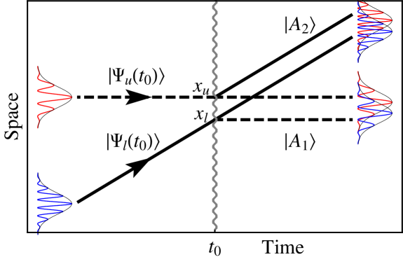
Figure 1: Separation Phase. This is a magnified view of the end of the interferometer which shows the upper and lower arms converging at the final beamsplitter at time $t_{0}$, and the resulting interference. The dashed and solid lines designate the components of the wavefunction in internal states $\left|A_{1}\right>$ and $\left|A_{2}\right>$, respectively. After the beamsplitter, each output port consists of a superposition of wavepackets from the upper and lower arm. Any offset $\mathbf{\Delta x}=\mathbf{x}_{l}-\mathbf{x}_{u}$ between the centers of the wavepacket contributions to a given output port results in a separation phase shift.

We write the wavefunction components after the beamsplitter in the form of Eq. (21):

$$\left|\Psi_{u}(t)\right> = \int\!d\mathbf{p}\sum_{i}\,c_{i}^{(u)}(\mathbf{p},t)\hat{G}_{u}\left|\mathbf{p}\right>\left|A_{i}\right>$$ (40)

$$\left|\Psi_{l}(t)\right> = \int\!d\mathbf{p}\sum_{i}\,c_{i}^{(l)}(\mathbf{p},t)\hat{G}_{l}\left|\mathbf{p}\right>\left|A_{i}\right>$$ (41)

where we invoked the short pulse limit so that $e^{-i\hat{H}_{2}\tau}\approx 1$. Next we time evolve the states using Eq. (32) assuming a perfect $\frac{\pi}{2}$ pulse and using the initial conditions given in Eqs. (38) and (39): namely, $c_{1}^{(u)}(\mathbf{p},t_{0})=c_{1}(\mathbf{p},t_{0})e^{i\theta_{u}}$ and $c_{2}^{(u)}(\mathbf{p},t_{0})=0$ for the upper arm and $c_{1}^{(l)}(\mathbf{p},t_{0})=0$ and $c_{2}^{(l)}(\mathbf{p},t_{0})=c_{2}(\mathbf{p},t_{0})e^{i\theta_{l}}$ for the lower arm.

$$\qquad\qquad\left|\Psi_{u}(t)\right> = \int\!d\mathbf{p}\,c_{1}(\mathbf{p},t_{0})\left\{\frac{1}{\sqrt{2}}\hat{G}_{u}\left|\mathbf{p}\right>\left|A_{1}\right>+\frac{-i}{\sqrt{2}}e^{i\phi_{L}(\mathbf{x}_{u})}\hat{G}_{u}\left|\mathbf{p}+\mathbf{k}\right>\left|A_{2}\right>\right\}e^{i\theta_{u}}$$ (42)

$$\qquad\qquad\left|\Psi_{l}(t)\right> = \int\!d\mathbf{p}\,c_{2}(\mathbf{p}+\mathbf{k},t_{0})\left\{\frac{-i}{\sqrt{2}}e^{-i\phi_{L}(\mathbf{x}_{l})}\hat{G}_{l}\left|\mathbf{p}\right>\left|A_{1}\right>+\frac{1}{\sqrt{2}}\hat{G}_{l}\left|\mathbf{p}+\mathbf{k}\right>\left|A_{2}\right>\right\}e^{i\theta_{l}}$$ (43)

We now project into position space and perform the $\mathbf{p}$ integrals,

$$\qquad\qquad\left<\mathbf{x}|\Psi_{u}(t)\right> = \frac{c_{1}(\mathbf{x}-\mathbf{x}_{u},t_{0})}{\sqrt{2}}\left\{e^{i\mathbf{p}_{u}\cdot(\mathbf{x}-\mathbf{x}_{u})}\left|A_{1}\right>-ie^{i\phi_{L}(\mathbf{x}_{u})}e^{i(\mathbf{p}_{u}+\mathbf{k})\cdot(\mathbf{x}-\mathbf{x}_{u})}\left|A_{2}\right>\right\}e^{i\theta_{u}}$$ (44)

$$\qquad\qquad\left<\mathbf{x}|\Psi_{l}(t)\right> = \frac{c_{2}(\mathbf{x}-\mathbf{x}_{l},t_{0})}{\sqrt{2}}\left\{-ie^{-i\phi_{L}(\mathbf{x}_{l})}e^{i(\mathbf{p}_{l}-\mathbf{k})\cdot(\mathbf{x}-\mathbf{x}_{l})}\left|A_{1}\right>+e^{i\mathbf{p}_{l}\cdot(\mathbf{x}-\mathbf{x}_{l})}\left|A_{2}\right>\right\}e^{i\theta_{l}}$$ (45)

where we identified the Fourier transformed amplitudes using $c_{i}(\mathbf{x}-\mathbf{x}_{c},t_{0})=\int\!d\mathbf{p}\,\left<\mathbf{x}-\mathbf{x}_{c}|\mathbf{p}\right>c_{i}(\mathbf{p},t_{0})$. The resulting interference pattern in position space is therefore

$$\left<\mathbf{x}|\Psi(t)\right> = \left<\mathbf{x}|\Psi_{u}(t)\right>+\left<\mathbf{x}|\Psi_{l}(t)\right>$$

$$= \frac{1}{\sqrt{2}}\left|A_{1}\right>\left\{c_{1}(\mathbf{x}-\mathbf{x}_{u},t_{0})e^{i\theta_{u}}e^{i\mathbf{p}_{u}\cdot(\mathbf{x}-\mathbf{x}_{u})}-i\,c_{2}(\mathbf{x}-\mathbf{x}_{l},t_{0})e^{i\theta_{l}}e^{-i\phi_{L}(\mathbf{x}_{l})}e^{i(\mathbf{p}_{l}-\mathbf{k})\cdot(\mathbf{x}-\mathbf{x}_{l})}\right\}$$

$$+ \frac{1}{\sqrt{2}}\left|A_{2}\right>\left\{c_{2}(\mathbf{x}-\mathbf{x}_{l},t_{0})e^{i\theta_{l}}e^{i\mathbf{p}_{l}\cdot(\mathbf{x}-\mathbf{x}_{l})}-i\,c_{1}(\mathbf{x}-\mathbf{x}_{u},t_{0})e^{i\theta_{u}}e^{i\phi_{L}(\mathbf{x}_{u})}e^{i(\mathbf{p}_{u}+\mathbf{k})\cdot(\mathbf{x}-\mathbf{x}_{u})}\right\}$$

The probability of finding the atom in either output port $\left|A_{1}\right>$ or $\left|A_{2}\right>$ is

$$\left|\left<A_{1}\right|\left<\mathbf{x}|\Psi(t)\right>\right|^{2} = \frac{\left|c_{1}\right|^{2}+\left|c_{2}\right|^{2}}{2}+\frac{1}{2}\left(i\,c_{1}\,c_{2}^{\ast}\,e^{i\Delta\phi_{1}}+c.c.\right)$$ (46)

$$\left|\left<A_{2}\right|\left<\mathbf{x}|\Psi(t)\right>\right|^{2} = \frac{\left|c_{1}\right|^{2}+\left|c_{2}\right|^{2}}{2}-\frac{1}{2}\left(i\,c_{1}\,c_{2}^{\ast}\,e^{i\Delta\phi_{2}}+c.c.\right)$$ (47)

with $c_{1}\equiv c_{1}(\mathbf{x}-\mathbf{x}_{u},t_{0})$ and $c_{2}\equiv c_{2}(\mathbf{x}-\mathbf{x}_{l},t_{0})$. For the total phase shift we find

$$\Delta\phi_{1} \equiv \Big{\{}\theta_{u}+\mathbf{p}_{u}\cdot(\mathbf{x}-\mathbf{x}_{u})\Big{\}}-\Big{\{}\theta_{l}-\phi_{L}(\mathbf{x}_{l})+(\mathbf{p}_{l}-\mathbf{k})\cdot(\mathbf{x}-\mathbf{x}_{l})\Big{\}}$$ (48)

$$= \underbrace{\theta_{u}-\Big{(}\theta_{l}-\phi_{L}(\mathbf{x}_{l})\Big{)}}_{\Delta\phi_{\text{propagation,1}}~{}+~{}\Delta\phi_{\text{laser,1}}}+\underbrace{\Big{.}\,\,\mathbf{\bar{p}}_{1}\cdot\mathbf{\Delta x}\,\,}_{\Delta\phi_{\text{separation,1}}}+\,\,\mathbf{\Delta p}\cdot(\mathbf{x}-\mathbf{\bar{x}})$$ (49)

and

$$\Delta\phi_{2} \equiv \Big{\{}\theta_{u}+\phi_{L}(\mathbf{x}_{u})+(\mathbf{p}_{u}+\mathbf{k})\cdot(\mathbf{x}-\mathbf{x}_{u})\Big{\}}-\Big{\{}\theta_{l}+\mathbf{p}_{l}\cdot(\mathbf{x}-\mathbf{x}_{l})\Big{\}}$$ (50)

$$= \underbrace{\Big{(}\theta_{u}+\phi_{L}(\mathbf{x}_{u})\Big{)}-\theta_{l}}_{\Delta\phi_{\text{propagation,2}}~{}+~{}\Delta\phi_{\text{laser,2}}}+\underbrace{\Big{.}\,\,\mathbf{\bar{p}}_{2}\cdot\mathbf{\Delta x}\,\,}_{\Delta\phi_{\text{separation,2}}}+\,\,\mathbf{\Delta p}\cdot(\mathbf{x}-\mathbf{\bar{x}})$$ (51)

where $\mathbf{\bar{p}}_{1}=\frac{\mathbf{p}_{u}+(\mathbf{p}_{l}-\mathbf{k})}{2}$ and $\mathbf{\bar{p}}_{2}=\frac{(\mathbf{p}_{u}+\mathbf{k})+\mathbf{p}_{l}}{2}$ are the average momenta in the $\left|A_{1}\right>$ (slow) and $\left|A_{2}\right>$ (fast) output ports, respectively. In general, the separation phase is

$$\Delta\phi_{\text{separation}}=\mathbf{\bar{p}}\cdot\mathbf{\Delta x}$$ (52)

which depends on the separation $\mathbf{\Delta x}\equiv\mathbf{x}_{l}-\mathbf{x}_{u}$ between the centers of the wavepackets from each arm as well as the average canonical momentum $\mathbf{\bar{p}}$ in the output port. We point out that even though the definitions (48) and (50) use the same sign convention as our previous expressions for laser (36) and propagation (20) phase in the sense of $(~{})_{\text{upper}}-(~{})_{\text{lower}}$, the separation vector $\mathbf{\Delta x}$ is defined as $(\mathbf{x})_{\text{lower}}-(\mathbf{x})_{\text{upper}}$.

Notice that the phase shift expressions (49) and (51) contain a position dependent piece $\mathbf{\Delta p}\cdot(\mathbf{x}-\mathbf{\bar{x}})$, where $\mathbf{\bar{x}}\equiv\frac{\mathbf{x}_{u}+\mathbf{x}_{l}}{2}$ and $\mathbf{\Delta p}=(\mathbf{p}_{u}+\mathbf{k})-\mathbf{p}_{l}=\mathbf{p}_{u}-(\mathbf{p}_{l}-\mathbf{k})$, owing to the fact that the contributions from each arm may have different momenta after the last beamsplitter. Typically this momentum difference is very small, so the resulting phase variation has a wavelength that is large compared to the spatial extent of the wavefunction. Furthermore, this effect vanishes completely in the case of spatially averaged detection over a symmetric wavefunction.

Finally, we show that the total phase shifts $\Delta\phi_{1}$ and $\Delta\phi_{2}$ for the two output ports are actually equal, as required by conservation of probability. According to Eqs. (49) and (51), the contributions to the total phase differ in the following ways:

$$\Big{(}\Delta\phi_{\text{propagation,1}}+\Delta\phi_{\text{laser,1}}\Big{)}-\Big{(}\Delta\phi_{\text{propagation,2}}+\Delta\phi_{\text{laser,2}}\Big{)} = \phi_{L}(\mathbf{x}_{l})-\phi_{L}(\mathbf{x}_{u})$$

$$= \mathbf{k}\cdot(\mathbf{x}_{l}-\mathbf{x}_{u})=\mathbf{k}\cdot\mathbf{\Delta x}$$

$$\Delta\phi_{\text{separation,1}}-\Delta\phi_{\text{separation,2}}=\mathbf{\bar{p}}_{1}\cdot\mathbf{\Delta x}-\mathbf{\bar{p}}_{2}\cdot\mathbf{\Delta x}=-\mathbf{k}\cdot\mathbf{\Delta x}$$

Together these results imply that $\Delta\phi_{1}=\Delta\phi_{2}$ and prove that the total interferometer phase shift $\Delta\phi_{\text{tot}}$ is independent of the output port.

The accuracy of the above formalism is dependent on the applicability of the aforementioned stationary phase approximation as well as the short pulse limit. The stationary phase approximation breaks down when the external Hamiltonian varies rapidly compared to the phase space width of the atom wavepacket. The short pulse limit requires that the atom’s velocity not change appreciably during the duration of the atom-light interaction. Both approximations are justified to a large degree for a typical light pulse atom interferometer, but in the most extreme high precision applications such as we consider here, important corrections are present. However, we emphasize that these errors due to finite pulse duration and wavepacket size are well-known, previously established backgrounds.

4 Applications in inertial navigation

The navigation problem is easily stated: How do we determine a platform’s trajectory as a function of time? In the 20th century, solutions to the problem have led to the development of exquisitely refined hardware systems and navigation algorithms. Today we take for granted that a hand-held GPS reciever can be used to obtain meter level position determination. When GPS is unavailable (for example, when satellites are not in view), position determination becomes much less accurate. In this case, stand-alone “black-box” inertial navigation systems, comprised of a suite of gyroscope and acclerometers, are used to infer position changes by integrating the outputs of these inertial force sensors. State-of-the-art commercial grade navigation systems have position drift errors of kilometers per hour of navigation time, significantly worse than the GPS solution. How can we close the performance gap between GPS and inertial systems? The way forward is improved instrumentation: better gyroscopes and accelerometers.

The light-pulse interferometry method is well suited to inertial applications. As shown in Section 3.1, the phase shift for the light pulse interferometer consists of contributions from path phases, optical interactions, and separation phases. However, for the sensitivity range of interest, the optical phase shifts dominate, and therefore $\Delta\phi_{tot}\approx\Delta\phi_{laser}$. In this case there is a straightforward interpretation for the operation of the sensor: the sensor registers the time evolution of the relative position of the atomic wavepackets with respect to the sensor case (defined by the opto-mechanical hardware for the laser beams) using optical interferometry. Since distances are measured in terms of the wavelength of light, and the atom is in a benign environment (spurious forces, such as from magnetic field gradients, are extremely small – below $10^{-10}g$), the sensors are characterized by superbly stable, low-noise operation.

The phase shift between the two paths is inferred by measuring the probability of finding the atoms in a given output port. Since we are only concerned with the optical phase shift, we can calculate the sensor output using Eq. (3). We see that for a standard $\pi/2-\pi-\pi/2$ excitation sequence [35], $\Delta\phi_{laser}={\bf k}_{1}\cdot({\bf x}_{1}^{u}-{\bf x}_{1}^{0})-{\bf k}_{2}\cdot({\bf x}_{2}^{u}-{\bf x}_{2}^{0})-{\bf k}_{2}\cdot({\bf x}_{2}^{l}-{\bf x}_{2}^{0})+{\bf k}_{3}\cdot({\bf x}_{3}^{l}-{\bf x}_{3}^{0})$ . Here the subscript indexes each of the three successive optical interactions, ${\bf x}_{i}^{u}$ and ${\bf x}_{i}^{l}$ are the semi-classical positions of the atom along the upper and lower paths, respectively, at the time of each interaction in a non-rotating, inertial coordinate system, ${\bf x}_{i}^{0}$ is the phase reference for the optical fields, and ${\bf k}_{i}$ is the propagation vector of the laser field associated with each pulse.

4.1 Gyroscope

Assuming the atoms have initial velocity ${\bf v}_{0}$ and the effective Raman propagation vectors initially have common orientations ${\bf k}_{0}$ which rotate with angular rate ${\bf\Omega}$, it is straightforward to show that $\Delta\phi_{laser}\approx{\bf k}_{0}\cdot(2{\bf v}_{0}\times{\bf\Omega})T^{2}$. This configuration is well-suited to precision measurements of platform rotations. This expression can be put in a form analogous to the Sagnac shift for optical interferometers by noting that for small rotation rates $\Omega$, $\mathbf{A}=\frac{\hbar}{m}({\bf k_{0}}\times{\bf v_{0}})T^{2}$ is the area enclosed by the interfering paths. Thus this shift can also be written in the Sagnac form $\phi=\frac{2m}{\hbar}\mathbf{\Omega}\cdot\mathbf{A}$ – proportional to the product of the enclosed area and rotation rate.

Gyroscopes built on this principle have achieved performance levels in the laboratory which compare favorably with state-of-the art gyroscopes, as shown in Figs. 2, 3, 4 and 5. Key figures of merit for gyroscope performance include gyroscope noise (often referred to as angle random walk), bias stability (stability of output for a null input) and scale factor stability (stability of the multiplier between the input rotation rate and output phase shift). The laboratory gyroscope illustrated below has achieved a demonstrated angle random walk of $3~{}\mu\text{deg}/\text{hr}^{1/2}$, bias stability of $60~{}\mu\text{deg}/\text{hr}$ (upper limit) and scale factor stability of 5 ppm (upper limit). Key drivers in the stability of the gyroscope outputs are the stability of the intensities used to drive the Raman transitions, and alignment stability of the Raman beam optical paths. Non-inertial phase shifts associated with magnetic field inhomogeneities and spurious AC Stark shifts are nulled using a case reversal technical where the propagation directions of the Raman beams are periodically reversed using electo-optic methods.

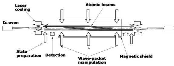
Figure 2: Schematic illustration of an atomic beam gyroscope.

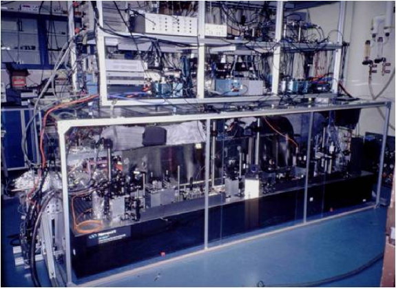
Figure 3: Photograph of gyroscope.

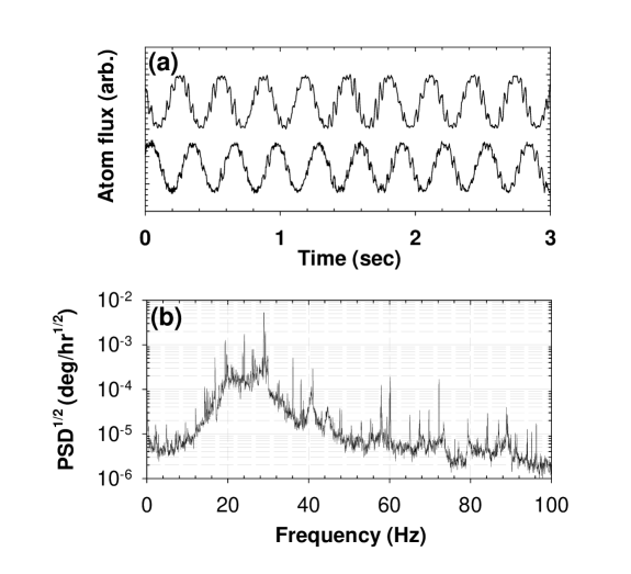
Figure 4: Gyroscope interference fringes (a) and power spectral density of gyroscope noise (b). The increase in noise in the 10-50 Hz band is due to technical rotation noise sources in the building (the gyroscope was mounted directly to the building floor). See Ref. [13].

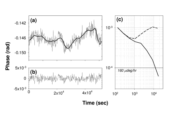
Figure 5: (a) Drift in case reversed gyroscope output with time and its correlation with instrument temperature (solid black). (b) Gyro noise output residual after subtracting temperature model. (c) Allan deviation of gyro output before and after temperature compensation (see Ref. [13]).

4.2 Accelerometer

If the platform containing the laser beams accelerates, or if the atoms are subject to a gravitational acceleration, the laser phase shift then contains acceleration terms $\Delta\phi={\bf k}_{0}\cdot{\bf a}T^{2}.$ For a stationary interferometer, with the laser beams vertically directed, this phase shift measures the acceleration due to gravity. Remarkably, part per billion level agreement has been demonstrated between the output of an atom interferometer gravimeter and a conventional, “falling-corner-cube” gravimeter. [14]. In the future, compact, geophysical ($10^{-8}$ $g$ accuracy) grade instruments should enable low cost gravity field surveys (see Fig. 6). For this type of instrument, laser cooling methods are used to initially prepare ensembles of roughly $10^{7}$ atoms at kinetic temperatures approaching 1 $\mu$K. At these low temperatures, the rms velocity spread of the atomic ensembles is a few cm/sec. Cold atom ensembles are then launched on ballistic trajectories. In this configuration, the time between laser pulses exceeds 100 msec, which means wavepackets separate by roughly 1 mm over the course of the interferometer sequence. The phase shift is read-out by detecting the number of atoms in each final state using resonance fluorescence and normalized detection methods.

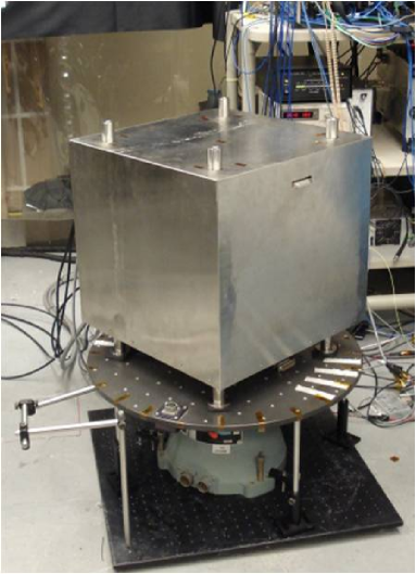
Figure 6: Compact accelerometer. This instrument supports accelerometer, gyroscope and gravity gradiometer operation modes. The compact accelerometer has demonstrated microGal sensitivity.

In general, both rotation and acceleration terms are present in the sensor outputs. For navigation applications, the rotation response needs to be isolated from the acceleration response. In practice, this is accomplished by using multiple atom sources and laser beam propagation axes. For example, for the gyroscope illustrated in Fig. 2, counter-propagating atom beams are used to isolate rotation induced phase shifts from acceleration induced shifts. It is interesting to note that the same apparatus is capable of simultaneous rotation and acceleration outputs – a significant benefit for navigation applications which require simultaneous output of rotation rate and acceleration for three mutually orthogonal axes. Since gyroscope and accelerometer operation rest on common principles and common hardware implementations, integration of sensors into a full inertial base is straightforward. Of course, particular hardware implementations depend on the navigation platform (e.g. ship, plane, land vehicle) and trajectory dynamics.

4.3 Gravity gradiometer

There is an additional complication in navigation system architecture for high accuracy navigation applications: the so-called “problem of the vertical.” Terrestrial navigation requires determining platform position in the gravity field of the Earth. Due to the Equivalence Principle, navigation system accelerometers do not distinguish between the acceleration due to gravity and platform acceleration. So in order to determine platform trajectory in an Earth-fixed coordinate system, the local acceleration due to gravity needs to be subtracted from accelerometer output in order to determine the acceleration of the vehicle with respect to the Earth. This means that the local acceleration due to gravity needs to be independently known. For example, existing navigation systems use a gravity map to make this compensation. However, in present systems, this map does not have enough resolution or accuracy for meter-level position determination. To give a feeling for orders of magnitude, a $10^{-7}$ error in knowledge of the local acceleration due to gravity integrates to meter-level position errors in 1 hour.

There are at least two paths forward: 1) better maps or 2) on-the-fly gravity field determination. Improved maps can be obtained with more precise surveys. On-the-fly determination seems impossible, due to the Equivalence Principle (since platform accelerations cannot be discriminated from the acceleration due to gravity). However, the outputs from a gravity gradiometer – an instrument which measures changes in the acceleration due to gravity over fixed baselines – can be used for this purpose. The idea is to integrate the gravity gradient over the inferred trajectory to determine gravity as a function of position. In principle, such an instrument can function on a moving platform, since platform accelerations cancel as a common mode when the output from spatially separated accelerometers are differenced to obtain the gradient. In practice, such a strategy places hard requirements on the stability of the component accelerometers: their responses need to be matched to an exceptional degree in order to discriminate gravity gradient induced accelerations (typically below 10^-9 $g$) from other sensor error sources.

Due to the stability of their acceleration outputs, a pair of light pulse accelerometers is well-suited to gravity gradient instrumentation. The basic idea is to simultaneously create two spatially separated interferometers using a common laser beam. In this way, technical acceleration noise of the measurement platform is a common-mode noise source which leads to near identical phase shifts in each accelerometer. On the other hand, a gravity gradient along the measurement axis results in a residual differential phase shift. This configuration has been used to measure the gravity gradient of the Earth, as well as the gravity gradient associated with nearby mass distributions, as illustrated in Fig. 7. Laboratory gravity gradiometers have achieved resolutions below 1 E (where 1 E = $10^{-9}$ sec^-2). This configuration has also been used to measure the Newtonian constant of gravity $G$ [15, 16, 17]. In future navigation systems, an ensemble of accelerometers, configured along independent measurement axes, could acquire the full gravity gradient tensor.

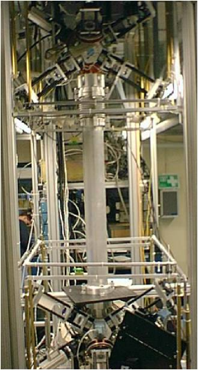
Figure 7: Vertical axis gravity gradiometer. Two atom interferometer accelerometers separated along a vertical measurement axis are simultaneously interrogated by a common set of Raman laser beams. This apparatus was used to measure $G$, Newton’s constant [15].

In addition to their role as navigation aids, gravity gradiometers have applications in geodesy and oil/mineral exploration. The idea here is that mass/density anomalies associated with interesting geophysical features (such as kimberlite pipes – in the case of diamond exploration – or salt domes – in the case of oil exploration) manifest as gravity anomalies. In some cases, these anomalies can be pronounced enough to be detected by a gravity gradiometer from an airborne platform. Atom-based gravity gradiometers appear to have competitive performance figures of merit for these applications as compared with existing technologies. For these applications, the central design challenge is realization of an instrument which has very good noise performance, but also is capable of sustained operation on a moving platform. Figs. 8, 9 illustrate a system currently under development for this purpose.

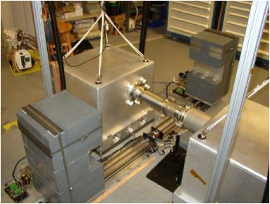
Figure 8: Gravity gradiometer with horizontal measurement axis. Raman beams propagate along the axis defined by the tube connecting each accelerometer housing.

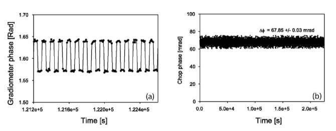
Figure 9: Gravity gradiometer response to a proof mass which is periodically brought in close proximity to one of the accelerometer regions. For the proof masses used for this demonstration, the apparatus is capable of resolving changes in $G$ at the $3\times 10^{-4}$ level [18].

5 Application to tests of the Equivalence Principle

Precision tests of the Equivalence Principle (EP) promise to provide insight into fundamental physics. Since the EP is one of the central axioms of general relativity (GR), these experiments are powerful checks of gravity and can tightly constrain new theories. Furthermore, EP experiments test for hypothetical fifth forces since many examples of new forces are EP–violating[19].

The Equivalence Principle has several forms, with varying degrees of universality. Here we consider tests of the Weak Equivalence Principle, which can be stated as follows: the motion of a body in a gravitational field in any local region of space-time is indistinguishable from its motion in a uniformly accelerated frame. This implies that the body’s inertial mass is equal to its gravitational mass, and that all bodies locally fall at the same rate under gravity, independent of their mass or composition.

The results of EP experiments are typically expressed in terms of the Eötvös parameter $\eta=\Delta a/\bar{a}$, where $\Delta a$ is the EP violating differential acceleration between the two test bodies and $\bar{a}$ is their average acceleration [20]. Currently, two conceptually different experiments set the best limits on the Equivalence Principle. Lunar Laser Ranging (LLR), which tests the EP by comparing the acceleration of the Earth and Moon as they fall toward the Sun, limits EP violation at $\eta=(-1.0\pm 1.4)\times 10^{-13}$ [21]. Recently, the Eöt-Wash group has set a limit of $\eta=(0.3\pm 1.8)\times 10^{-13}$ using an Earth-based torsion pendulum apparatus[22]. Several proposed satellite missions aim to improve on these limits by observing the motion of macroscopic test bodies in orbit around the Earth[23, 24]. Here we discuss our effort to perform a ground-based EP test using individual atoms with a goal of measuring $\eta\sim 10^{-15}$. Instead of macroscopic test masses, we compare the simultaneous acceleration under gravity of freely-falling cold atom clouds of ⁸⁷​Rb and ⁸⁵​Rb using light-pulse atom interferometry [25].

Light-pulse atom interferometers have already been used to make extremely accurate inertial force measurements in a variety of configurations, including gyroscopes, gradiometers, and gravimeters. For example, the local gravitational acceleration $g$ of freely-falling Cs atoms was measured with an accuracy $\sim 10^{-9}g$ [14]. Gravity gradiometers have been used to suppress noise as well as many systematic errors that are present in absolute $g$ measurements by comparing the acceleration of two displaced samples of atoms. A differential measurement of this kind was used to measure the Newtonian constant of gravity $G$ with an accuracy of $\sim 3\times 10^{-3}G$ [15]. The EP measurement we describe here benefits from an analogous differential measurements strategy, where in this case the common-mode noise suppression arises from a comparison between two co-located isotopes of different mass, rather than between spatially separated atoms as in a traditional gradiometer.

5.1 Proposed experiment overview

The proposed experiment ideally consists of simultaneously observing the free-fall motion of the two Rb isotopes in the absence of all non-gravitational forces. To this end, the measurement is performed inside a $10~{}\text{cm}$ diameter by $8.8~{}\text{m}$ long cylindrical ultra high vacuum chamber. To maximize their free-fall time, the atoms are launched in a vertical fountain geometry from the bottom of the chamber. Light-pulse atom interferometry is performed while the atoms are in free-fall, and the resulting phase shift is sensitive to the atoms’ acceleration. Figure 10 is a space-time diagram depicting the trajectories that each atom follows during the free-fall interferometry sequence.

To maximize the cancellation of spurious effects, both the ⁸⁷​Rb and ⁸⁵​Rb atom clouds are launched at the same time and are made to follow the same trajectories as closely as possible. We launch both isotopes from the same magnetic trap in order to minimize any differences between their initial positions and velocities. As a result of the small isotope shift between ⁸⁷​Rb and ⁸⁵​Rb, we are able to use the same laser pulses to simultaneously manipulate them during the interferometer sequence (see Fig. 10). Using the same laser makes the apparatus insensitive to pulse timing jitter and dramatically reduces the phase noise stability requirements of the lasers.

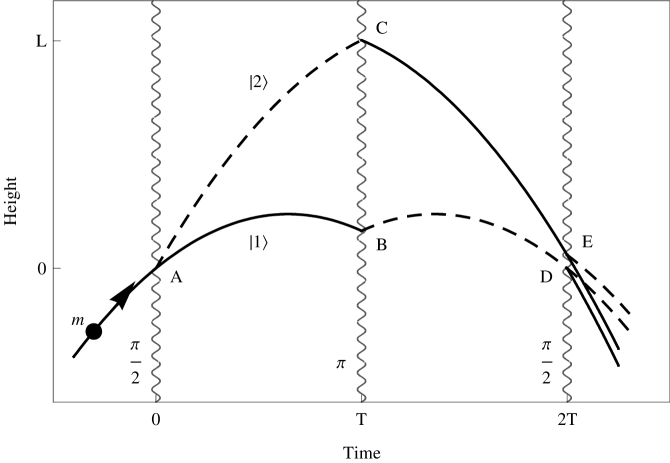
Figure 10: Space–time diagram for a single atom of mass $m$ during the interferometer pulse sequence. The atom is launched with velocity $v_{z}$ from the bottom of the vacuum system. At time $t=0$, a $\frac{\pi}{2}$ (beamsplitter) pulse is applied to coherently divide the atom wavefunction. After a time $T$, a $\pi$ (mirror) pulse is applied that reverses the relative velocity between the wavefunction components. A final $\frac{\pi}{2}$ (beamsplitter) pulse at time $2T$ results in interference between the two space–time paths. The interferometer phase shift is inferred by measuring the probability of detecting the atom in either state $\left|1\right>$ (solid line) or state $\left|2\right>$ (dashed line). Note that points $D$ and $E$ are in general spatially separated in the presence of non-uniform forces, leading to a separation phase shift.

A single measurement of acceleration in our atom interferometer consists of three steps: atom cloud preparation, interferometer pulse sequence, and detection. In the first step a sub-microkelvin cloud of $\sim 10^{7}$ atoms is formed using laser cooling and evaporative cooling in a TOP trap [26]. This dilute ensemble of cold atoms is then launched vertically with velocity $v_{z}\sim 13~{}\text{m}/\text{s}$ by transferring momentum from laser light using an accelerated optical lattice potential [27]. This technique allows for precise control of the launch velocity and, because it is a coherent process, it avoids heating the cloud via spontaneous emission.

In the second phase of the measurement, the atoms follow free-fall trajectories and the interferometry is performed. A sequence of laser pulses serve as beamsplitters and mirrors that coherently divide each atom’s wavepacket and then later recombine it to produce interference (see Fig. 10). The atom beamsplitter is typically implemented using a stimulated two-photon process (Raman or Bragg transitions), resulting in a net momentum transfer of $\mathbf{k_{\text{eff}}}=\mathbf{k_{2}}-\mathbf{k_{1}}\approx 2\mathbf{k_{2}}$ at each interaction. Since the acceleration sensitivity of the interferometer is proportional to the effective momentum $\hbar k_{\text{eff}}$ transferred to the atom during interactions with the laser, we intend to take advantage of more sophisticated atom optics. Large momentum transfer (LMT) beamsplitters with $\hbar k_{\text{eff}}=24\hbar k$ have been demonstrated [28], and up to $100\hbar k$ may be possible. Promising LMT beamsplitter candidates include optical lattice manipulations [27], sequences of Raman pulses [29] and adiabatic passage methods [30].

The third and final step of each acceleration measurement is atom detection. At the end of the interferometer sequence, each atom is in a superposition of the two output velocity states, as shown by the diverging paths on the right in Fig. 10. These two final velocity states are directly analogous to the two output ports of a Mach-Zehnder light interferometer after the final recombining beamsplitter. As with a light interferometer, the probability that an atom will be found in a particular output port depends on the relative phase acquired along the two paths of the atom interferometer. Since the output states differ in velocity by $\sim\hbar k_{\text{eff}}/m$, they spatially separate over time. After an appropriate drift time, the two velocity groups can be separately resolved, and the populations can be then measured by fluorescence imaging.

We now consider the expected sensitivity of our differential ⁸⁷​Rb–⁸⁵​Rb accelerometer. Recent atom interferometers have demonstrated sensor noise levels limited only by the quantum projection noise of the atoms (atom shot noise) [31]. Assuming a time–average atom flux of $n=10^{6}~{}\text{atoms}/\text{s}$, the resulting shot noise–limited phase sensitivity is $\sim\frac{1}{\sqrt{n}}=10^{-3}~{}\text{rad}/\sqrt{\text{Hz}}$. The phase shift in an atom interferometer due to a constant acceleration $g$ is $\Delta\phi=k_{\text{eff}}gT^{2}$ [4]. Taking advantage of the $L\approx 8.8~{}\text{m}$ vacuum system allows for a long interrogation time of up to $T=1.34~{}\text{s}$. Finally, using $\hbar k_{\text{eff}}=10\hbar k$ LMT beamsplitters results in an acceleration sensitivity of $\sim 7\times 10^{-13}~{}g/\sqrt{\text{Hz}}$ and a precision of $<10^{-15}g$ after $\sim 1~{}\text{day}$ of integration. In the most conservative case, constraining ourselves to conventional $2\hbar k$ atom optics leads to a precision of $<10^{-15}g$ after $\sim 1~{}\text{month}$ of integration. This estimate is based on realistic extrapolations from current performance levels, which are at $10^{-10}g$ [15].

5.2 Error model

An accurate test of the EP requires a thorough understanding of potential backgrounds. To reach the goal sensitivity, we must control spurious accelerations to $<10^{-15}g$. Systematic errors at this level can arise from many sources, including gravity gradients, Earth’s rotation, and electromagnetic forces. To calculate these contributions to the phase shift, we follow the prescription outlined in Section 3. We take the atom’s Lagrangian in the lab frame to be

$$L=\frac{1}{2}m(\dot{\mathbf{r}}+\mathbf{\Omega}\times(\mathbf{r}+\mathbf{R}_{e}))^{2}-m\phi(\mathbf{r}+\mathbf{R}_{e})-\frac{1}{2}\alpha\mathbf{B(\mathbf{r})}^{2}$$ (53)

where $\mathbf{r}$ is the position of the atom in the lab frame, $\mathbf{R}_{e}=(0,0,R_{e})$ is the radius of the Earth, $\mathbf{\Omega}=(0,\Omega_{y},\Omega_{z})$ is the Earth’s rotation rate, and $\phi(\mathbf{r})$ is the gravitational potential. In the chosen coordinate system, $z$ is the vertical direction in the lab and $\mathbf{\Omega}$ lies in the $y$-$z$ plane. We then expand $\phi$ in a Taylor series about $\mathbf{R}_{e}$,

$$\phi(\mathbf{r}+\mathbf{R}_{e})=-\left(\mathbf{g}\cdot\mathbf{r}+\frac{1}{2!}(T_{ij})r_{i}r_{j}+\frac{1}{3!}(Q_{ijk})r_{i}r_{j}r_{k}+\frac{1}{4!}(S_{ijkl})r_{i}r_{j}r_{k}r_{l}\right)$$ (54)

where Earth’s gravity field is $\mathbf{g}\equiv-\nabla\phi(\mathbf{R}_{e})$, the gravity gradient tensor is $T_{ij}\equiv\partial_{j}g_{i}$, the second gradient tensor is $Q_{ijk}\equiv\partial_{k}\partial_{j}g_{i}$, the third gradient tensor is $S_{ijkl}\equiv\partial_{l}\partial_{k}\partial_{j}g_{i}$, and repeated indices are summed over. Since $\mathbf{\hat{z}}$ is in the vertical direction in the lab we have that $\mathbf{g}=(0,0,-g)$ and $g=9.8~{}\text{m}/\text{s}^{2}$. The interferometer follows a fountain geometry which is approximately one-dimensional along the $z$-direction, so we only include $Q_{zzz}$ and $S_{zzzz}$ and safely ignore the other second and third gradient tensor terms. Likewise, in this analysis we assume that off-diagonal gradient tensor terms $T_{ij}$ with $i\neq j$ are small and can be ignored (this is exactly true for a perfectly spherical Earth). The effects of higher-order moments of the gravitational field are treated separately using a perturbative calculation as described in Section 5.2.1.

Because magnetic fields can cause significant systematic errors, the atoms are prepared in one of the magnetic field insensitive clock states ($\left|m_{F}=0\right>$ states). The residual energy shift in a magnetic field $\mathbf{B}$ is then $U_{B}=\frac{1}{2}\alpha\mathbf{B}^{2}$, where $\alpha$ is the second order Zeeman shift coefficient. We consider magnetic fields of the form

$$\mathbf{B(\mathbf{r})}=\left(B_{0}+\frac{\partial B}{\partial z}z\right)\mathbf{\hat{z}}$$ (55)

where $B_{0}$ is a constant bias magnetic field, and $\frac{\partial B}{\partial z}$ is the gradient of the background magnetic field. While this linear model is sufficient for slowly varying fields, in Section 5.2.2 we describe a perturbative calculation that can account for more complicated magnetic field spatial profiles.

We do not include additional electromagnetic forces in the Lagrangian as their accelerations are well below our systematic threshold. For neutral atoms, electric fields are generally not a concern since the atom’s response is second order. Furthermore, electric fields are easily screened by the metallic vacuum chamber, leading to negligibly small phase shifts. Short range effects due to the Casimir [32] force or local patch potentials [33] are also negligible since the atoms are kept far ($>1~{}\text{cm}$) from all surfaces throughout the experiment.

As explained in Section 3.2, we point out that the phase shift derived from Eq. 1 is only exactly correct for Lagrangians that are second order in position and velocity. When this is not true, as is the case in Eq. 53 when $Q_{ijk}\neq 0$ and $S_{ijkl}\neq 0$, the semiclassical formalism breaks down and there are quantum corrections to the phase shift. However, these corrections depend on the size of the atom wavepacket compared to the length scale of variation of the potential, and are typically negligible for wavepackets $\sim 1~{}\text{mm}$ in size.

To analytically determine the trajectories $\mathbf{r}(t)$, we solve the Euler-Lagrange equations using a power series expansion in $t$:

$$r_{i}(t)=\sum_{n=0}^{N}a_{in}(t-t_{0})^{n}\qquad\qquad(i=1,2,3)$$ (56)

The coefficients $a_{in}$ are determined recursively after substitution into the equations of motion. This expansion converges quickly as long as $\Omega T\ll 1$ and $\left|\frac{r^{n}}{g}\frac{\partial^{n}g}{\partial r^{n}}\right|\ll 1$. For our apparatus with characteristic length $r\sim 10~{}\text{m}$ and time $T\sim 1~{}\text{s}$ these conditions are easily met, since $\Omega T\sim 10^{-4}~{}\text{rad}$ and $\left|\frac{r^{n}}{g}\frac{\partial^{n}g}{\partial r^{n}}\right|\sim\left(\frac{r}{R_{e}}\right)^{n}\lesssim 10^{-6}$ assuming a spherical Earth. With these trajectories and the interferometer geometry shown in Fig. 10 we obtain the following expressions for the phase shift in the slow (state $\left|1\right>$) output port:

$$\Delta\phi_{\text{propagation}} = \frac{1}{\hbar}((S_{AC}+S_{CE})-(S_{AB}+S_{BD}))$$ (57)

$$\Delta\phi_{\text{laser}} = \phi_{L}(\mathbf{r}_{A},0)-\phi_{L}(\mathbf{r}_{C},T)-\phi_{L}(\mathbf{r}_{B},T)+\phi_{L}(\mathbf{r}_{D},2T)$$ (58)

$$\Delta\phi_{\text{separation}} = \frac{1}{2\hbar}(\mathbf{p}_{D}+\mathbf{p}_{E})\cdot(\mathbf{r}_{D}-\mathbf{r}_{E})$$ (59)

where $S_{ij}$ is the classical action along the path segment between points $\mathbf{r}_{i}$ and $\mathbf{r}_{j}$, and $\mathbf{p}_{i}=\partial_{\mathbf{\dot{r}}}L(\mathbf{r}_{i})$ is the classical canonical momentum at point $\mathbf{r}_{i}$ after the final beamsplitter. The laser phase shift at each interaction point is

$$\phi_{L}(\mathbf{r},t)=\mathbf{k_{\text{eff}}}\cdot\mathbf{r}-\omega_{\text{eff}}t+\phi_{0}$$ (60)

where $\mathbf{k_{\text{eff}}}$ and $\omega_{\text{eff}}$ are the effective propagation vector and frequency, respectively, for whatever atom–laser interaction is used to implement the atom optics. In the case of the stimulated two–photon processes mentioned earlier, $\mathbf{k_{\text{eff}}}=\mathbf{k_{2}}-\mathbf{k_{1}}$ and $\omega_{\text{eff}}=\omega_{2}-\omega_{1}=(k_{2}-k_{1})/c.$

$\begin{array}[]{lccc}\hline\cr\\ &\qquad\qquad\text{Phase shift}&\qquad\text{Size (rad)}&\qquad\text{Fractional size}\\ \hline\cr\hline\cr\\ 1&-k_{\text{eff}}gT^{2}&-2.85\times 10^{8}&1.00\\ 2&k_{\text{eff}}R_{e}\Omega_{y}^{2}T^{2}&6.18\times 10^{5}&2.17\times 10^{\text{-3}}\\ 3&-k_{\text{eff}}T_{zz}v_{z}T^{3}&1.58\times 10^{3}&5.54\times 10^{\text{-6}}\\ 4&\frac{7}{12}k_{\text{eff}}gT_{zz}T^{4}&-9.21\times 10^{2}&3.23\times 10^{\text{-6}}\\ 5&-3k_{\text{eff}}v_{z}\Omega_{y}^{2}T^{3}&-5.14&1.80\times 10^{\text{-8}}\\ 6&2k_{\text{eff}}v_{x}\Omega_{y}T^{2}&3.35&1.18\times 10^{\text{-8}}\\ 7&\frac{7}{4}k_{\text{eff}}g\Omega_{y}^{2}T^{4}&3.00&1.05\times 10^{\text{-8}}\\ 8&-\frac{7}{12}k_{\text{eff}}R_{e}T_{zz}\Omega_{y}^{2}T^{4}&2.00&7.01\times 10^{\text{-9}}\\ 9&-\frac{\hbar k_{\text{eff}}^{2}}{2m}T_{zz}T^{3}&7.05\times 10^{\text{-1}}&2.48\times 10^{\text{-9}}\\ 10&\frac{3}{4}k_{\text{eff}}gQ_{zzz}v_{z}T^{5}&9.84\times 10^{\text{-3}}&3.46\times 10^{\text{-11}}\\ 11&-\frac{7}{12}k_{\text{eff}}Q_{zzz}v_{z}^{2}T^{4}&-7.66\times 10^{\text{-3}}&2.69\times 10^{\text{-11}}\\ 12&-\frac{7}{4}k_{\text{eff}}R_{e}\Omega_{y}^{4}T^{4}&-6.50\times 10^{\text{-3}}&2.28\times 10^{\text{-11}}\\ 13&-\frac{7}{4}k_{\text{eff}}R_{e}\Omega_{y}^{2}\Omega_{z}^{2}T^{4}&-3.81\times 10^{\text{-3}}&1.34\times 10^{\text{-11}}\\ 14&-\frac{31}{120}k_{\text{eff}}g^{2}Q_{zzz}T^{6}&-3.39\times 10^{\text{-3}}&1.19\times 10^{\text{-11}}\\ 15&-\frac{3\hbar k_{\text{eff}}^{2}}{2m}\Omega_{y}^{2}T^{3}&-2.30\times 10^{\text{-3}}&8.06\times 10^{\text{-12}}\\ 16&\frac{1}{4}k_{\text{eff}}T_{zz}^{2}v_{z}T^{5}&2.19\times 10^{\text{-3}}&7.68\times 10^{\text{-12}}\\ 17&-\frac{31}{360}k_{\text{eff}}gT_{zz}^{2}T^{6}&-7.53\times 10^{\text{-4}}&2.65\times 10^{\text{-12}}\\ 18&3k_{\text{eff}}v_{y}\Omega_{y}\Omega_{z}T^{3}&2.98\times 10^{\text{-4}}&1.05\times 10^{\text{-12}}\\ 19&-k_{\text{eff}}\Omega_{y}\Omega_{z}y_{0}T^{2}&-7.41\times 10^{\text{-5}}&2.60\times 10^{\text{-13}}\\ 20&-\frac{3}{4}k_{\text{eff}}R_{e}Q_{zzz}v_{z}\Omega_{y}^{2}T^{5}&-2.14\times 10^{\text{-5}}&7.50\times 10^{\text{-14}}\\ 21&\frac{31}{60}k_{\text{eff}}gR_{e}Q_{zzz}\Omega_{y}^{2}T^{6}&1.47\times 10^{\text{-5}}&5.17\times 10^{\text{-14}}\\ 22&\frac{3}{2}k_{\text{eff}}T_{zz}v_{z}\Omega_{y}^{2}T^{5}&-1.42\times 10^{\text{-5}}&5.00\times 10^{\text{-14}}\\ 23&-\frac{7}{6}k_{\text{eff}}T_{zz}v_{x}\Omega_{y}T^{4}&1.08\times 10^{\text{-5}}&3.81\times 10^{\text{-14}}\\ 24&-2k_{\text{eff}}T_{xx}\Omega_{y}x_{0}T^{3}&-6.92\times 10^{\text{-6}}&2.43\times 10^{\text{-14}}\\ 25&-\frac{7\hbar k_{\text{eff}}^{2}}{12m}Q_{zzz}v_{z}T^{4}&-6.84\times 10^{\text{-6}}&2.40\times 10^{\text{-14}}\\ 26&-\frac{7}{6}k_{\text{eff}}T_{xx}v_{x}\Omega_{y}T^{4}&-5.42\times 10^{\text{-6}}&1.90\times 10^{\text{-14}}\\ 27&-\frac{31}{60}k_{\text{eff}}gT_{zz}\Omega_{y}^{2}T^{6}&4.90\times 10^{\text{-6}}&1.72\times 10^{\text{-14}}\\ 28&k_{\text{eff}}T_{xx}v_{z}\Omega_{y}^{2}T^{5}&4.75\times 10^{\text{-6}}&1.67\times 10^{\text{-14}}\\ 29&\frac{3\hbar k_{\text{eff}}^{2}}{8m}gQ_{zzz}T^{5}&4.40\times 10^{\text{-6}}&1.55\times 10^{\text{-14}}\\ 30&\frac{31}{360}k_{\text{eff}}R_{e}T_{zz}^{2}\Omega_{y}^{2}T^{6}&1.63\times 10^{\text{-6}}&5.74\times 10^{\text{-15}}\\ 31&-\frac{31}{90}k_{\text{eff}}gT_{xx}\Omega_{y}^{2}T^{6}&-1.63\times 10^{\text{-6}}&5.74\times 10^{\text{-15}}\\ 32&\frac{\hbar k_{\text{eff}}^{2}}{8m}T_{zz}^{2}T^{5}&9.78\times 10^{\text{-7}}&3.43\times 10^{\text{-15}}\\ 33&-\frac{\hbar k_{\text{eff}}\alpha B_{0}(\partial_{z}B)T^{2}}{m}&-7.67\times 10^{\text{-8}}&2.69\times 10^{\text{-16}}\\ 34&\frac{31}{60}k_{\text{eff}}gS_{zzzz}v_{z}^{2}T^{6}&-7.52\times 10^{\text{-8}}&2.64\times 10^{\text{-16}}\\ 35&-\frac{1}{4}k_{\text{eff}}S_{zzzz}v_{z}^{3}T^{5}&3.64\times 10^{\text{-8}}&1.28\times 10^{\text{-16}}\\ 36&\frac{31}{72}k_{\text{eff}}T_{zz}Q_{zzz}v_{z}^{2}T^{6}&-3.13\times 10^{\text{-8}}&1.10\times 10^{\text{-16}}\\ \hline\cr\end{array}$

Table 1: Phase shift response for a single atom interferometer $\frac{\pi}{2}-\pi-\frac{\pi}{2}$ sequence given the Lagrangian in Eq. 53. Column 3 shows the fractional size of each term compared to the acceleration signal $k_{\text{eff}}gT^{2}$. All terms with fractional phase shift $>10^{-16}$ are included. The numbers are for a ⁸⁷​Rb interferometer with the following parameters: $k_{\text{eff}}=2k=2\cdot\frac{2\pi}{780~{}\text{nm}}$, $T_{zz}=-2g/R_{e}$, $T_{xx}=T_{yy}=g/R_{e}$, $Q_{zzz}=6g/R_{e}^{2}$, $S_{zzzz}=-24g/R_{e}^{3}$, $R_{e}=6.72\times 10^{6}\text{m}$, $B_{0}=100~{}\text{nT}$, and $\partial_{z}B=0.1~{}\text{nT}/\text{m}$. The Earth’s rotation rate is given by $\Omega_{y}=\Omega\cos{\theta_{\text{Lat}}}$ and $\Omega_{z}=\Omega\sin{\theta_{\text{Lat}}}$ with $\Omega=7.27\times 10^{-5}~{}\text{rad}/\text{s}$ and $\theta_{\text{Lat}}=37.4$ degrees North latitude. The initial position of the atom in the lab is taken as $\mathbf{r}(0)=(x_{0},y_{0},0)$, with $x_{0}=1~{}\text{mm}$ and $y_{0}=1~{}\text{mm}$. The initial velocity is $\mathbf{\dot{r}}(0)=(v_{x},v_{y},v_{z})$, with $v_{x}=1~{}\text{mm}/\text{s}$, $v_{y}=1~{}\text{mm}/\text{s}$, and $v_{z}=13.2~{}\text{m}/\text{s}$.

Using the above method, we computed the phase shift response for a single atom interferometer, and the results are shown in Table 1. The values of the experimental parameters used to generate this list are representative of the $8.8~{}\text{m}$ apparatus described previously. Many of these terms are common to both species, and in order obtain our $<10^{-15}g$ sensitivity, we rely on their common mode cancellation. In Table 2 we compute the differential phase shift between a ⁸⁷​Rb and a ⁸⁵​Rb interferometer. The two species have different masses $m$ and second order Zeeman coefficients $\alpha$, as well as potentially different launch kinematics $\mathbf{r}(0)$ and $\mathbf{\dot{r}}(0)$. To create Table 2, we parameterized the launch kinematics with a differential velocity $\mathbf{\delta v}=(\delta v_{x},\delta v_{y},\delta v_{z})$ and initial position $\mathbf{\delta r}=(\delta x,\delta y,\delta z)$ between the centroids of the two isotope clouds. Residual systematic phase errors are the result of differential accelerations that arise from gravity gradients, second gravity gradients, coriolis and centrifugal forces, and magnetic forces on the atoms.

$\begin{array}[]{lccc}\hline\cr\\ &\qquad\qquad\text{Phase shift}&\qquad\text{Size (rad)}&\qquad\text{Fractional size}\\ \hline\cr\hline\cr\\ 1&-\frac{1}{2}\left(\frac{1}{\text{m85}}-\frac{1}{m_{87}}\right)\hbar k_{\text{eff}}^{2}T_{zz}T^{3}&1.66\times 10^{\text{-2}}&5.83\times 10^{\text{-11}}\\ 2&2k_{\text{eff}}\delta v_{x}\Omega_{y}T^{2}&3.35\times 10^{\text{-3}}&1.18\times 10^{\text{-11}}\\ 3&-k_{\text{eff}}T_{zz}\delta v_{z}T^{3}&1.44\times 10^{\text{-4}}&5.05\times 10^{\text{-12}}\\ 4&-\frac{3}{2}\left(\frac{1}{m_{85}}-\frac{1}{m_{87}}\right)\hbar k_{\text{eff}}^{2}\Omega_{y}^{2}T^{3}&-5.40\times 10^{\text{-5}}&1.90\times 10^{\text{-13}}\\ 5&-3k_{\text{eff}}\Omega_{y}^{2}\delta v_{z}T^{3}&-4.68\times 10^{\text{-6}}&1.64\times 10^{\text{-14}}\\ 6&-k_{\text{eff}}T_{zz}\delta zT^{2}&8.93\times 10^{\text{-7}}&3.14\times 10^{\text{-15}}\\ 7&-k_{\text{eff}}\delta y\Omega_{y}\Omega_{z}T^{2}&-7.41\times 10^{\text{-7}}&2.60\times 10^{\text{-15}}\\ 8&3k_{\text{eff}}\delta v_{y}\Omega_{y}\Omega_{z}T^{3}&2.98\times 10^{\text{-7}}&1.05\times 10^{\text{-15}}\\ 9&-\frac{7}{12}\left(\frac{1}{m_{85}}-\frac{1}{m_{87}}\right)\hbar k_{\text{eff}}^{2}Q_{zzz}v_{z}T^{4}&-1.61\times 10^{\text{-7}}&5.65\times 10^{\text{-16}}\\ 10&\frac{3}{8}\left(\frac{1}{m_{85}}-\frac{1}{m_{87}}\right)\hbar k_{\text{eff}}^{2}gQ_{zzz}T^{5}&1.03\times 10^{\text{-7}}&3.63\times 10^{\text{-16}}\\ 11&-\left(\frac{\alpha_{85}}{m_{85}}-\frac{\alpha_{87}}{m_{87}}\right)\hbar k_{\text{eff}}B_{0}(\partial_{z}B)T^{2}&-9.94\times 10^{\text{-8}}&3.49\times 10^{\text{-16}}\\ 12&-2k_{\text{eff}}T_{xx}\delta x\Omega_{y}T^{3}&-6.92\times 10^{\text{-8}}&2.43\times 10^{\text{-16}}\\ \hline\cr\end{array}$

Table 2: Differential phase shift between ⁸⁷​Rb and ⁸⁵​Rb. To create the differential phase shift list we parameterized the launch kinematics with a differential velocity $(\delta v_{x}=1~{}\mu\text{m}/\text{s},\delta v_{y}=1~{}\mu\text{m}/\text{s},\delta v_{z}=12~{}\mu\text{m}/\text{s})$ and position $(\delta x=1~{}\mu\text{m},\delta y=1~{}\mu\text{m},\delta z=10~{}\text{nm})$ between the centroids of the two isotope clouds. All other parameters are the same as in Table 1. Column 3 shows the fractional size of each term compared to the acceleration signal $k_{\text{eff}}gT^{2}$. We include all terms with a fractional phase shift $>10^{-16}$.

As justified below, we expect to achieve experimental parameters that reduce the majority of the systematic errors below our experimental threshold. However, the first several terms in Table 2 are still too large. In order to further reduce these backgrounds, we can employ propagation reversal to suppress all terms $\propto k_{\text{eff}}^{2}$. This well–known technique entails reversing the laser propagation vector $\mathbf{k_{\text{eff}}}\longrightarrow-\mathbf{k_{\text{eff}}}$ on subsequent trials and then subtracting the two results [15]. This suppresses terms 1, 4, 9, and 10 by $\Delta k_{\text{eff}}/k_{\text{eff}}$, where $\Delta k_{\text{eff}}$ is the error in $k_{\text{eff}}$ made as a result of the reversal. Reducing these terms below our systematic threshold requires $\Delta k_{\text{eff}}/k_{\text{eff}}<10^{-5}$. The main acceleration signal and all other terms linear in $k_{\text{eff}}$ are not suppressed by this subtraction.

After propagation vector reversal, the last important background phase shifts arise from the differential coriolis and centrifugal acceleration between the isotopes (Table 2 terms 2, 5, 7, and 8), and from the Earth’s gravity gradient (Table 2 terms 3 and 6). We discuss the techniques used to control these remaining systematics in Section 5.3.

5.2.1 Gravity Inhomogeneities

The Taylor series expansion of the gravitational potential (see Eq. 54) is a good approximation of the coarse structure of Earth’s gravity on length scales of $\sim R_{e}$, the radius of the Earth. However, local gravity can also vary on much shorter length scales in a way that depends on the specific mass distribution surrounding the experiment, and these gravity inhomogeneities can result in spurious phase shifts. Since these inhomogeneities can be rapidly spatially varying, the Taylor series expansion is not well-suited for their description. Instead, we leverage the fact that these inhomogeneities are typically small in magnitude and solve for the induced phase shift using first–order perturbation theory [3]. This linearization allows us to make a Fourier decomposition of the phase shift response in terms of the spatial wavelengths of the local $g$–field.

First, we assume a one-dimensional gravitational potential perturbation of the form $\delta\phi(z)$. The gravity field perturbation along the vertical ($z$) direction is defined as $\delta g_{z}(z)\equiv-\partial_{z}\delta\phi$ and may be written as

$$\delta g_{z}(z)=\int\widetilde{\delta g}_{z}(\lambda)e^{\frac{i2\pi z}{\lambda}}d\lambda$$ (61)

where $\widetilde{\delta g}_{z}(\lambda)$ is the Fourier component of a gravity perturbation with wavelength $\lambda$. The total phase shift due to gravity inhomogeneities summed over all wavelengths is

$$\Delta\phi_{g}=\int T_{gz}(\lambda)\widetilde{\delta g}_{z}(\lambda)d\lambda$$ (62)

where $T_{gz}(\lambda)$ is the interferometer’s gravity perturbation response function. Qualitatively, the response to short wavelengths is suppressed since the interferometer averages over variations that are smaller than its length [34]. The response is flat for wavelengths longer than the scale of the interferometer, and in the limit where $\lambda\sim R_{e}$ this analysis smoothly approaches the results of our Taylor series calculation described above.

Figure 11: Differential gravity response function versus spatial wavelength $\lambda$ between simultaneous ⁸⁷​Rb and ⁸⁵​Rb interferometers. Short wavelengths are averaged over by each individual interferometer, while long wavelength inhomogeneities cancel as a common-mode between the two species. This response curve assumes identical launch kinematics for the two isotopes.

For the ⁸⁷​Rb–⁸⁵​Rb EP measurement, we are interested in the differential phase response between the isotopes. Figure 11 shows the differential response function $\Delta T_{gz}(\lambda)\equiv\left|(T_{gz})_{87}-(T_{gz})_{85}\right|$ for gravity inhomogeneities. Once again, short wavelength variations are suppressed since each interferometer spatially averages over a $\sim 10~{}\text{m}$ region. The peak response occurs at a length scale set by the spatial separation of the arms of a single interferometer $\Delta z=\frac{\hbar k_{\text{eff}}}{m}T\sim 16~{}\text{mm}$. Perfect differential cancellation between isotopes is not achieved because the spatial separation of the arms is mass dependent. Additionally, the long wavelength differential response is suppressed because the differences between the isotope trajectories are negligible when compared to variations with length scales much longer than $\Delta z$.

The differential response curve allows us to compute systematic errors arising from the specific gravity environment of our interferometer. Quantitative estimates of these effects requires knowledge of the local $\delta g_{z}(z)$, which may be obtained through a combination of modelling and characterization. The atom interferometer itself can be used as a precision gravimeter for mapping $\delta g_{z}(z)$ in situ. By varying the launch velocity, initial vertical position, and interrogation time $T$, the position of each gravity measurement can be controlled.

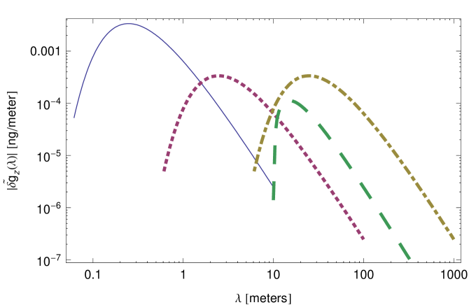
Figure 12: The magnitude power spectra of the local gravitational field, $\widetilde{\delta g}_{z}$, for several example sources. The solid (blue) curve is a $10^{-2}~{}\text{kg}$ point source, 10 cm from the center of the interferometer. Similarly, the dotted (purple) curve is a 1 kg source at 1 m and the dash-dotted (yellow) curve is 1000 kg at 10 m. The long-dashed (green) curve is a thin 10 m long rod of mass 10 kg, parallel to the interferometer, whose center is 1 m from the interferometer.

Figure 11 shows that the differential ⁸⁷​Rb–⁸⁵​Rb interferometer is maximally sensitive to short wavelength ($\lambda\sim 1-10~{}\text{cm}$) gravitational inhomogeneities. To investigate the impact of local uneven mass distributions on the experiment, we compute the spectrum $\widetilde{\delta g}_{z}(\lambda)$ of various sources at different distances from the interferometer. These results are shown in Fig. 12. When combined with our response function (Fig. 11), we see that for typical mass inhomogeneities, only those that are within a few centimeters of the interferometer can cause potentially significant systematic phase shifts. These nearby inhomogeneities result in phase errors of $\sim 10^{-6}~{}\text{rad}$, which is slightly above our target sensitivity. It will therefore be especially important for the EP measurement that we characterize the local $g$–field at the centimeter scale.

5.2.2 Magnetic field inhomogeneities

The linear expansion of $\mathbf{B}$ in Eq. 55 approximates large scale variation of the magnetic field. However, local field inhomogeneities may exist on short length scales due to the presence of nearby magnetic materials. These variations are not well approximated by a Taylor series expansion. Using the same procedure described above for gravity inhomogeneities, we write the local magnetic field as

$$B(z)=\int\widetilde{B}_{z}(\lambda)e^{\frac{i2\pi z}{\lambda}}d\lambda$$ (63)

where $\widetilde{B}_{z}(\lambda)$ is the Fourier component of a field perturbation with wavelength $\lambda$. The total phase shift from magnetic field inhomogeneities is

$$\Delta\phi_{B}=\int T_{Bz}(\lambda)\widetilde{B}_{z}(\lambda)d\lambda$$ (64)

Here $T_{Bz}(\lambda)$ is the interferometer’s magnetic inhomogeneity response function.

As with gravity above, we compute the differential response function $\Delta T_{Bz}(\lambda)\equiv\left|(T_{Bz})_{87}-(T_{Bz})_{85}\right|$ between ⁸⁷​Rb and ⁸⁵​Rb (see Fig. 13). The differential response arises because the isotopes have different second order Zeeman coefficients $\alpha$, as well as different masses. This sensitivity curve drives our magnetic shield design requirements, as discussed in Section 5.3.3.

Figure 13: Differential magnetic field response function between simultaneous ⁸⁷​Rb and ⁸⁵​Rb interferometers. Short wavelengths are averaged over by each individual interferometer, while long wavelength inhomogeneities cancel as a common-mode between the two species. This response curve assumes identical launch kinematics for the two isotopes.

5.3 Controlling potential systematic errors

5.3.1 Rotation of the Earth

The largest systematic term in the phase shift expansion for a dual species differential interferometer after propagation reversal is due to the rotation of the Earth. Specifically, a differential acceleration due to the coriolis force occurs if the isotopes have different transverse velocities $\delta v_{x}$ (Table 2, term 2). Reducing this phase shift below our systematic threshold would require $\delta v_{x}<10^{-11}~{}\text{m}/\text{s}$, which is challenging. However, this specification can be relaxed by artificially making the rotation rate zero.

To a good approximation, the atoms are only affected by the Earth’s rotation through their coupling to the laser, so the coriolis acceleration can be eliminated by rotating the laser in the opposite direction of the Earth’s rotation. In order to calculate the effect of this rotation compensation, we performed the phase shift calculation using a rotating $\mathbf{k_{\text{eff}}}$. Following the work of [14], we use a retro-reflection configuration to deliver the laser beams $\mathbf{k}_{1}$ and $\mathbf{k}_{2}$ to the atoms. We rotate $\mathbf{k_{\text{eff}}}$ by actuating the retro-reflection mirror. As a result, the incoming beam remains pointing along the $z$-direction and only the reflected beam rotates. With this configuration, $\mathbf{k_{\text{eff}}}$ is given by

$$\mathbf{k_{\text{eff}}}=-2k\mathbf{\hat{n}}(\mathbf{\hat{n}}\cdot\mathbf{\hat{k}})$$ (65)

where $\mathbf{\hat{n}}$ is the time-dependent unit normal vector of the retro-reflection mirror, and $\mathbf{\hat{k}}$ is a unit vector in the direction of the fixed delivery beam. Notice that the direction of $\mathbf{k_{\text{eff}}}$ rotates as desired, but its length now depends on angle.

The resulting phase shift list appears in Table 3, with $\delta\Omega_{y}$ and $\delta\Omega_{z}$ the errors in the applied counter-rotation rate. Assuming a transverse velocity difference of $\delta v_{x}\sim 1~{}\mu\text{m}/\text{s}$, these rotation compensation errors must be kept below $10^{-5}\Omega_{\text{Earth}}\approx 1~{}\text{nrad}/\text{s}$. Methods for measuring angles with nanoradian precision have already been demonstrated [36]. In order to actuate the mirror at this level of precision we can use commercially available sub-nm accurate piezo-electric actuators along with active feedback.

Notice that not all rotation-related phase errors are removed by rotation compensation. Terms that arise from the differential centrifugal acceleration between the isotopes (e.g., Table 3 terms 3 and 4) are not suppressed. Physically, this is a consequence of the fact that the retro-reflection mirror that we use to change the laser’s angle is displaced from the center of rotation of the Earth by $R_{e}$. Therefore, although we can compensate for the angle of the laser by counter-rotating, the retro-reflection mirror remains attached to the rotating Earth, leading to a centrifugal acceleration of the phase fronts. After propagation reversal, the only term of this type that is significant is $\sim k_{\text{eff}}\Omega_{y}^{2}\delta v_{z}T^{3}$ (Table 3 term 4). However, this term is smaller than and has the same scaling with experimental control parameters as the gravity gradient phase shift (Table 3 term 2), so the constraints described in Section 5.3.2 to suppress the gravity gradient terms are sufficient to control this centrifugal term as well.

One potential obstacle in achieving the required transverse velocity constraint of $\delta v_{x}\sim 1~{}\mu\text{m}/\text{s}$ is the expected micro-motion the atoms experience in the TOP magnetic trap prior to launch [37]. Micro-motion orbital velocities in a tight TOP trap such as ours can approach $\sim 1~{}\text{cm}/\text{s}$ in the transverse plane. Although the differential orbital velocities are suppressed by the ⁸⁷​Rb–⁸⁵​Rb mass ratio, the resulting $\delta v_{x}\sim 100~{}\mu\text{m}/\text{s}$ is still too large. This problem can potentially be solved by adiabatically reducing the magnetic field gradient and increasing the rotating field frequency prior to launch.

$\begin{array}[]{lccc}\hline\cr\\ &\qquad\qquad\text{Phase shift}&\qquad\text{Size (rad)}&\qquad\text{Fractional size}\\ \hline\cr\hline\cr\\ 1&-\frac{1}{2}\left(\frac{1}{m_{85}}-\frac{1}{m_{87}}\right)\hbar k_{\text{eff}}^{2}T_{zz}T^{3}&1.66\times 10^{\text{-2}}&5.83\times 10^{\text{-11}}\\ 2&-k_{\text{eff}}T_{zz}\delta v_{z}T^{3}&1.44\times 10^{\text{-4}}&5.05\times 10^{\text{-12}}\\ 3&-\frac{3}{2}\left(\frac{1}{m_{85}}-\frac{1}{m_{87}}\right)\hbar k_{\text{eff}}^{2}\Omega_{y}^{2}T^{3}&-5.40\times 10^{\text{-5}}&1.90\times 10^{\text{-13}}\\ 4&-3k_{\text{eff}}\Omega_{y}^{2}\delta v_{z}T^{3}&-4.68\times 10^{\text{-6}}&1.64\times 10^{\text{-14}}\\ 5&-k_{\text{eff}}T_{zz}\delta zT^{2}&8.93\times 10^{\text{-7}}&3.14\times 10^{\text{-15}}\\ 6&-\frac{7}{12}\left(\frac{1}{m_{85}}-\frac{1}{m_{87}}\right)\hbar k_{\text{eff}}^{2}Q_{zzz}v_{z}T^{4}&-1.61\times 10^{\text{-7}}&5.65\times 10^{\text{-16}}\\ 7&\frac{3}{8}\left(\frac{1}{m_{85}}-\frac{1}{m_{87}}\right)\hbar k_{\text{eff}}^{2}Q_{zzz}gT^{5}&1.03\times 10^{\text{-7}}&3.63\times 10^{\text{-16}}\\ 8&-\left(\frac{\alpha_{85}}{m_{85}}-\frac{\alpha_{87}}{m_{87}}\right)\hbar k_{\text{eff}}B_{0}(\partial_{z}B)T^{2}&-9.94\times 10^{\text{-8}}&3.49\times 10^{\text{-16}}\\ 9&k_{\text{eff}}T_{xx}\delta x\Omega_{y}T^{3}&3.46\times 10^{\text{-8}}&1.22\times 10^{\text{-16}}\\ 10&-2k_{\text{eff}}\delta v_{x}\delta\Omega_{y}T^{2}&-3.35\times 10^{\text{-8}}&1.18\times 10^{\text{-16}}\\ \hline\cr\end{array}$

Table 3: Differential phase shift list with rotation compensation. Terms 1, 3, 6, and 7 will be suppressed by the propagation reversal technique described in Section 5.2.

5.3.2 Gravity gradients

The largest systematic background after rotation compensation is due to the gravity gradient along the vertical direction of the apparatus ($T_{zz}=\partial_{z}g_{z}$). Since gravity is not uniform, the two isotopes experience a different average acceleration if their trajectories are not identical. This effect causes a differential phase shift proportional to the initial spatial separation and initial velocity difference between the isotopes (see Table 3, terms 2 and 5). Assuming a spherical Earth model, the gravity gradient felt by the atoms is $T_{zz}\sim 3\times 10^{-16}g/\text{nm}$, which means that the initial vertical position difference between the isotopes $\delta z$ must be $<1~{}\text{nm}$ and the initial vertical velocity difference $\delta v_{z}$ must be $<1~{}\text{nm}/\text{s}$ in order to reduce the systematic phase shift beneath our threshold.

The experiment is designed to initially co-locate the two isotope clouds at the nm level by evaporative cooling both species in the same magnetic trap. For trapping, we use the state $\left|F=2,m_{F}=2\right>$ for ⁸⁷​Rb and $\left|F=3,m_{F}=3\right>$ for ⁸⁵​Rb since these states have the same magnetic moment [38]. The mass difference between the isotopes leads to a differential trap offset in the combined magnetic and gravitational potential given by

$$\Delta z_{\text{trap}}=\frac{g\Delta m}{\mu_{B}B^{\prime\prime}}$$ (66)

where $\Delta m$ is the ⁸⁷​Rb–⁸⁵​Rb mass difference, $B^{\prime\prime}$ is the magnetic field curvature of the trap, and $\mu_{B}$ is the Bohr magneton. Our TOP magnetic trap is designed to provide a field curvature $B^{\prime\prime}\sim 4\times 10^{5}~{}\text{Gauss}/\text{cm}^{2}$ which reduces the trap offset to $\Delta z_{\text{trap}}\approx 10~{}\text{nm}$. The resulting systematic error is $\sim 10^{-14}g$, but it can be subtracted during the analysis given a knowledge of $\Delta z_{\text{trap}}$ at the $\sim 10\%$ level. This offset can be inferred from a measurement of the field curvature $B^{\prime\prime}$ of the trap (e.g., by measuring the trap oscillation frequency). The gravity gradient must also be known, but this can be characterized in situ by using the interferometer as a gradiometer [15].

Control of the gravity gradient phase shift (Table 3 term 2) requires that the differential launch velocity be $\delta v_{z}\leq 1~{}\text{nm}/\text{s}$. Therefore we cannot employ standard launch techniques (e.g., moving molasses) since the velocity uncertainty is fundamentally limited by the photon recoil velocity $v_{R}\sim 6~{}\text{mm}/\text{s}$ due to spontaneous emission. Instead, the atoms are launched using an accelerated optical lattice potential [27]. We launch the two species using the same far-detuned ($\sim 200\text{GHz}$) optical lattice, coherently transferring $\sim 2200\hbar k$ of momentum to each cloud. Because the two species have different masses, they have different Bloch oscillation times $\tau_{B}=\frac{\hbar k_{\text{eff}}}{ma}$, where $a$ is the lattice acceleration. As a result, after adiabatically ramping down the lattice potential, the two species are in different momentum eigenstates since they have absorbed a different number of photons. The differential velocity after launch is then

$$\delta v_{L}=\hbar k_{\text{eff}}\left(\frac{N_{85}}{m_{85}}-\frac{N_{87}}{m_{87}}\right)$$ (67)

where $N_{85}$ and $N_{87}$ are the number of photons transferred to ⁸⁵​Rb and ⁸⁷​Rb, respectively. We choose the integers $N_{85}=2168$ and $N_{87}=2219$ such that their ratio is as close to the isotope mass ratio as possible, resulting in $\delta v_{L}\sim 12~{}\mu\text{m}/\text{s}$. After launch, we can perform a velocity selective transition to pick out a common class from the overlapping distributions of the two isotopes, which at the expense of atom number could conceivably allow us to achieve our differential velocity constraint.

There are several additional ways to reduce the gravity gradient systematics beyond precise control of the launch kinematics. We can implement a 4-pulse sequence ($\frac{\pi}{2}-\pi-\pi-\frac{\pi}{2}$) which suppresses all phase shift terms $\propto T^{3}$ at the cost of an order one loss in acceleration sensitivity [5]. This eliminates the velocity dependent gravity gradient phase shifts but would still require that we maintain tight control over the initial differential vertical position between the isotope clouds. Secondly, we can potentially reduce the local gravity gradient $T_{zz}$ by applying appropriate trim masses around the apparatus. It has been shown [34] that in principle a local mass distribution can effectively cancel the gravity gradient of the Earth for a $10~{}\text{m}$-scale apparatus. Reducing $T_{zz}$ by an order of magnitude would relax our initial position constraint to the level provided by the expected value of $\Delta z_{\text{trap}}$, thereby removing the requirement for subtraction during data analysis.

5.3.3 Magnetic fields

The magnetic field phase shift appearing in Table 3 (term 8) constrains the maximum allowed linear field gradient to $\partial_{z}B<0.1~{}\text{nT}/\text{meter}$. In the interferometer region, the measured gradient of the Earth’s field is $\sim 3~{}\mu\text{T}/\text{m}$, and therefore we require a shielding ratio of at least $\sim 5\times 10^{4}$. In addition to suppressing the field gradient, the magnetic response function (see Fig. 13) indicates that the field must be uniform on length scales $\sim 1~{}\text{cm}$. Large magnetic shields with similar performance have been demonstrated [39]. The magnetic shielding for our interferometer region is provided by a three–layer concentric cylindrical shield made of high permeability material. To maintain a pristine magnetic environment, we use an aluminum vacuum chamber and non-magnetic materials inside the shielded region.

In order to verify the performance of the magnetic shield, we must characterize the field. As with gravity inhomogeneities, the atom interferometer can be used to map the local magnetic field in situ, in this case by using a magnetic field sensitive ($m_{F}\neq 0$) state [40].

6 Conclusion

In these notes we have given an overview of the light-pulse method, and discussed applications to inertial navigation and a test of the Equivalence Principle. As the field continues to progress, we see two trends evolving. First, a steady evolution in the technology associated with laser manipulation of atoms will lead to progressive development of compact, field-ready inertial sensors. Such developments include integrated photonics packages for the laser and optics paths, and integrated optics bench and vacuum systems. On the other hand, continued evolution of high performance science instruments will extend the physics reach of this technology. For example, next generation light-pulse atom interference systems appear capable of placing superb limits on atom charge neutrality [41], making terrestrial tests of General Relativity [34, 42], and possibly detecting low frequency gravitational waves [43, 44].

References

• [1] \TITLEAtom Interferometry \ADLIBedited by P. Berman, (Academic Press, San Diego) 1997.
• [2] \BYD. W. Keith, C. R. Ekstrom, Q. A. Turchette, \atqueD. E. Pritchard \INPhys. Rev. Lett.6619912693 - 2696.
• [3] \BYP. Storey \atqueC. Cohen-Tannoudji \INJournal de Physique II419941999.
• [4] \BYK. Bongs, R. Launay, \atqueM. Kasevich \INAppl Phys. B842006599.
• [5] \BYB. Dubetsky \atqueM. A. Kasevich \INPhys. Rev. A742006023615.
• [6] \BYC. J. Borde \INGen. Rel. Grav.362004475.
• [7] \BYJae-Hoo Gweon \atqueJeong-Ryeol Choi \INJournal of the Korean Physical Society4220033.
• [8] \BYC. Antoine \INAppl. Phys. B842006585-597.
• [9] \BYM. Jansen \TITLEAtom interferometry with cold metastable helium, Ph.D. Thesis, Technische Universiteit Eindhoven (2007).
• [10] \BYKathryn Moler, David S. Weiss, Mark Kasevich \atqueSteven Chu \INPhys. Rev. A451992342-348.
• [11] \BYA. F. Bernhardt \atqueB. W. Shore \INPhys. Rev. A2319813.
• [12] \BYL. Allen \atqueJ. H. Eberly \TITLEOptical Resonance and Two-Level Atoms, \ADLIB(Dover Publications, Inc., New York) 1987.
• [13] \BYD. S. Durfee, Y. K. Shaham \atqueM. A. Kasevich \INPhys. Rev. Lett.972006240801.
• [14] \BYA. Peters, K. Y. Chung, \atqueS. Chu \INMetrologia38200125.
• [15] \BYJ. B. Fixler et al. \INScience315200774.
• [16] \BYJ. Fixler \TITLEAtom Interferometer-Based Gravity Gradiometer Measurements, Ph.D. Thesis, Yale University (2003).
• [17] \BYA. Bertoldi et al. \INEur. Phys. J. D402006271-279.
• [18] \BYG. Biedermann \TITLEGravity Tests, Differential Accelerometry and Interleaved Clocks with Cold Atom Interferometers, Ph.D. Thesis, Stanford University (2007).
• [19] \BYE. Fischbach. et al. \INMetrologia291992213-2.
• [20] \BYC. M. Will \INLiving Rev. Relativity920063. \ADLIBURL http://www.livingreviews.org/lrr-2006-3.
• [21] \BYJ. G. Williams et al. \INPhys. Rev. Lett.932004261101.
• [22] \BYS. Schlamminger, K.-Y. Choi, T. A. Wagner, J. H. Gundlach, \atqueE. G. Adelberger. \INPhys. Rev. Lett.932008041101.
• [23] \BYJ. Mester, R. Torii, P. Worden, N. Lockerbie, S. Vitale \atqueC. W. F. Everitt. \INClass. Quantum Grav.1820012475 2486.
• [24] \BYP. Touboul, B. Foulon, L. Lafargue \atqueG. Metris. \INActa Astronautic507433-443.
• [25] \BYM. Kasevich \atqueS. Chu. \INPhys. Rev. Lett.671991181.
• [26] \BYWolfgang Petrich et al. \INPhys. Rev. Lett.74199517. \BYC. Pethick \atqueH. Smith \TITLEBose-Einstein Condensation in Dilute Gases, \ADLIB(Cambridge Univ. Pr., New York) 2002.
• [27] \BYJ. H. Denschlag et al. \INJ. Phys. B: At. Mol. Opt. Phys.3520023095.
• [28] \BYH. Mueller, S.-w. Chiow, Q. Long, S. Herrmann, \atqueS. Chu. \ADLIBarXiv:0712.1990v1.
• [29] \BYJ. M. McGuirk et al. \INPhys. Rev. Lett.8520004498.
• [30] \BYM. Weitz et al. \INPhys. Rev. Lett.7319942563.
• [31] \BYG. Santarelli et al. \INPhys. Rev. Lett.8219994619. \BYJ. McGuirk et al. \INOpt. Lett.262001364. \BYS. Bize et al. \INJ. Phys. B: At. Mol. Opt. Phys.382005449-468.
• [32] \BYJ. M. Obrecht, R. J. Wild, M. Antezza, L. P. Pitaevskii, S. Stringari \atqueE. A. Cornell \INPhys. Rev. Lett.982007063201.
• [33] \BYJ. M. McGuirk, D. M. Harber, J. M. Obrecht \atqueE. A. Cornell \INPhys. Rev. A692004062905.
• [34] \BYS. Dimopoulos, P. W. Graham, J. M. Hogan \atqueM. A. Kasevich \ADLIBarXiv:0802.4098 [hep-ph].
• [35] \BYMark Kasevich \atqueSteven Chu \INPhys. Rev. Lett.671991181-184.
• [36] \BYM. Pisani \atqueM. Astrua \INAppl. Opt.4520061725-1729.
• [37] \BYJ. H. Müller, O. Morsch, D. Ciampini, M. Anderlini, R. Mannella, \atqueE. Arimondo \INPhys. Rev. Lett.8520004454.
• [38] \BYI. Bloch, M. Greiner, O. Mandel, T. Hänsch, \atqueT. Esslinger \INPhys. Rev. A642001021402.
• [39] \BYT. Bitter et al. \INNucl. Instrum. Meth. A3091991521.
• [40] \BYT. Kurosu et al. \INJpn. J. Appl. Phys.412002L586-L588.
• [41] \BYA. Arvanitaki, S. Dimopoulos, A. A. Geraci, J. Hogan, \atqueM. Kasevich \ADLIBarXiv:0711.4636 [hep-ph].
• [42] \BYS. Dimopoulos, P. W. Graham, J. M. Hogan \atqueM. A. Kasevich \INPhys. Rev. Lett.982007111102.
• [43] \BYS. Dimopoulos, P. W. Graham, J. M. Hogan, M. A. Kasevich \atqueS. Rajendran \ADLIBarXiv:0712.1250 [gr-qc].
• [44] \BYS. Dimopoulos, P. W. Graham, J. M. Hogan, M. A. Kasevich \atqueS. Rajendran \ADLIBarXiv:0806.2125 [gr-qc].