The cycle–convergence of restarted GMRES for normal matrices is sublinear

E. Vecharynski Department of Mathematical and Statistical Sciences, University of Colorado Denver, Denver, CO 80217 (yaugen.vecharynski@ucdenver.edu, julien.langou@ucdenver.edu).    J. Langou11footnotemark: 1
Abstract

We prove that the cycle–convergence of the restarted GMRES applied to a system of linear equations with a normal coefficient matrix is sublinear.

keywords:
Restarted GMRES, convergence, normal, diagonalizable, sublinear, superlinear.
AMS:
65F10.

1 Introduction

The generalized minimal residual method (GMRES) was originally introduced by Saad and Schultz [12] in 1986, and has become a popular method for solving non-Hermitian systems of linear equations

(1) $$Ax=b,\quad A\in\mathbb{C}^{n\times{n}},\quad b\in\mathbb{C}^{n}.$$

GMRES is classified as a Krylov subspace (projection) iterative method. At every new iteration $i$, GMRES constructs an approximation $x_{i}$ to the exact solution of (1), such that the $2$-norm of the corresponding residual vector $r_{i}=b-Ax_{i}$ is minimized over the affine space $r_{0}+A\mathcal{K}_{i}\left(A,r_{0}\right)$, i.e.

(2) $$r_{i}=\displaystyle\min_{u\in\mathcal{K}_{i}\left(A,r_{0}\right)}\|r_{0}-Au\|,$$

where $\mathcal{K}_{i}\left(A,r_{0}\right)$ is the $i$-dimensional Krylov subspace

$$\mathcal{K}_{i}\left(A,r_{0}\right)=\mbox{span}\{r_{0},Ar_{0},\dots,A^{i-1}r_{0}\}$$

induced by the matrix $A$ and the initial residual vector $r_{0}=b-Ax_{0}$ with $x_{0}$ being an initial approximate solution of (1).

As usual, in a linear setting, a notion of minimality is adjoint to some orthogonality condition. In our case, the minimization (2) is equivalent to forcing the new residual vector $r_{i}$ to be orthogonal to the subspace $A\mathcal{K}_{i}\left(A,r_{0}\right)$ (also known as the Krylov residual subspace). In practice, for a large problem size, the latter orthogonality condition results in a costly procedure of orthogonalization against the expanding Krylov residual subspace. Orthogonalization together with storage requirement makes the GMRES method complexity and storage prohibitive for practical application. A straightforward treatment for this complication is the so-called restarted GMRES [12].

The restarted GMRES, or GMRES($m$), is based on restarting GMRES after every $m$ iterations. At each restart, we use the latest approximate solution as the initial approximation for the next GMRES run. Within this framework a single run of $m$ GMRES iterations is called a GMRES($m$) cycle, $m$ is called the restart parameter. Consequently, restarted GMRES can be regarded as a sequence of GMRES($m$) cycles. When the convergence happens without any restart occurring, the algorithm is known as full GMRES.

Dealing with the restarted GMRES, our interest will shift towards the residual vectors $r_{k}$ at the end of every $k$-th GMRES($m$) cycle (as opposed to the residual vectors $r_{i}$ (2) at each iteration of the original algorithm).

Definition 1 (cycle–convergence).

We define the cycle–convergence of restarted GMRES ($m$) as the norm of the residual vectors $\|r_{k}\|$ at the end of every $k$-th GMRES($m$) cycle.

We note that each $r_{k}$ satisfies the local minimality condition

(3) $$r_{k}=\displaystyle\min_{u\in\mathcal{K}_{m}\left(A,r_{k-1}\right)}\|r_{k-1}-Au\|,$$

where $\mathcal{K}_{m}\left(A,r_{k-1}\right)$ is the $m$-dimensional Krylov subspace produced at the $k$-th GMRES($m$) cycle,

(4) $$\mathcal{K}_{m}\left(A,r_{k-1}\right)=\mbox{span}\{r_{k-1},Ar_{k-1},\dots,A^{m-1}r_{k-1}\}.$$

The price paid for the reduction of the computational work, as follows from (3) and (4), is the loss of global optimality (2). Although (3) implies a monotonic decrease of the norms of the residual vectors $r_{k}$, GMRES($m$) can stagnate [12, 17]. This is in contrast with full GMRES which is guaranteed to converge to the exact solution of (1) in $n$ steps (assuming exact arithmetic). However, a proper choice of a preconditioner or/and a restart parameter, e.g. [5, 6, 11], can significantly accelerate the convergence of GMRES($m$), thus making the method practically attractive.

While a lot of efforts have been put into the characterization of the convergence of full GMRES, e.g. [3, 4, 7, 8, 10, 14, 15], our understanding of the behavior of GMRES($m$) is far from complete, leaving us with more questions than answers, e.g. [5]. In this manuscript, we prove that the cycle–convergence of restarted GMRES for normal matrices is sublinear. This statement means that the reduction in the norm of the residual vector at the current GMRES($m$) cycle cannot be better than the reduction at the previous cycle.

The current manuscript was inspired by ideas introduced in the technical report [16] by I. Zavorin. In this work the author shows that, at every step of GMRES, a diagonalizable matrix $A$ and its Hermitian transpose $A^{H}$ yield the same worst-case behavior, and derives a necessary condition (the so-called cross-equality) for the worst-case right-hand side vector. We inherit the mathematical tools for our analysis from [16], as well as [10, 17], and give their brief description, slightly adapted to the case of the restarted GMRES and a normal matrix $A$, in Section 2. The main result of the sublinear cycle–convergence is proved in Section 3. In Section 4, the behavior of GMRES($m$) in the nonnormal case is discussed.

2 Krylov matrix, its pseudoinverse and spectral factorization

Throughout the manuscript we will assume (unless otherwise explicitly stated) $A$ to be nonsingular and normal, i.e. $A$ allows the decomposition

(5) $$A=V\Lambda V^{H},$$

where $\Lambda\in\mathbb{C}^{n\times{n}}$ is a diagonal matrix with the diagonal elements being the nonzero eigenvalues of $A$, and $V\in\mathbb{C}^{n\times{n}}$ is a unitary matrix of the corresponding eigenvectors.

Let us denote the $k$-th cycle of GMRES($m$) applied to the system (1) with the initial residual vector $r_{k-1}$ as GMRES($A$, $m$, $r_{k-1}$), $1\leq m\leq n-1$. We assume that the residual vector $r_{k}$, produced at the end of GMRES($A$, $m$, $r_{k-1}$), is nonzero.

According to (3) a run of GMRES($A$, $m$, $r_{k-1}$) entails the Krylov subspace $\mathcal{K}_{m}\left(A,r_{k-1}\right)$ (4). For each $\mathcal{K}_{m}\left(A,r_{k-1}\right)$ we define a matrix $K\left(A,r_{k-1}\right)\in\mathbb{C}^{n\times{(m+1)}}$, such that

(6) $$K\left(A,r_{k-1}\right)=\left[r_{k-1}\quad Ar_{k-1}\quad\dots\quad A^{m}r_{k-1}\right],\quad k=1,2,\dots,q,$$

where $q$ is the total number of GMRES($m$) cycles.

The matrix (6) is called the Krylov matrix. We will say that $K\left(A,r_{k-1}\right)$ corresponds to the cycle GMRES($A$, $m$, $r_{k-1}$). Note that the columns of $K\left(A,r_{k-1}\right)$ span the next, $(m+1)$-dimensional, Krylov subspace $\mathcal{K}_{m+1}(A,r_{k-1})$. By the assumption that $r_{k}\neq 0$,

$$\mbox{rank}\left(K\left(A,r_{k-1}\right)\right)=m+1.$$

This latter equality allows us to introduce the Moore-Penrose pseudoinverse of the matrix $K\left(A,r_{k-1}\right)$,

$$K^{\dagger}\left(A,r_{k-1}\right)=\left(K^{H}\left(A,r_{k-1}\right)K\left(A,r_{k-1}\right)\right)^{-1}K^{H}\left(A,r_{k-1}\right)\in\mathbb{C}^{{(m+1)}\times{n}},$$

which is well-defined and unique. The following lemma shows that the first column of $\left(K^{\dagger}\left(A,r_{k-1}\right)\right)^{H}$ is the next residual vector $r_{k}$ up to a scaling factor.

Lemma 2.

Given $A\in\mathbb{C}^{n\times{n}}$ (not necessarily normal) and the full rank Krylov matrix $K\left(A,r_{k-1}\right)\in\mathbb{C}^{n\times{(m+1)}}$, corresponding to the cycle GMRES($A$, $m$, $r_{k-1}$) for any $k=1,2,\dots,q$. Then

(7) $$\left(K^{\dagger}\left(A,r_{k-1}\right)\right)^{H}e_{1}=\frac{1}{\left\|r_{k}\right\|^{2}}r_{k},$$

where $e_{1}=\left[1\quad 0\quad\dots\quad 0\right]^{T}\in\mathbb{R}^{m+1}$.

Proof. See Ipsen [10, Theorem 2.1], as well as [2, 13]. $\square$

Another important idea, mentioned in [10] and intensively used in [16, 17], provides the so-called spectral factorization of the Krylov matrix $K\left(A,r_{k-1}\right)$ into three components, each one encapsulating separately the information on eigenvalues of $A$, its eigenvectors and the previous residual vector $r_{k-1}$.

Lemma 3.

Let $A\in\mathbb{C}^{n\times{n}}$ satisfying (5). Then the Krylov matrix $K\left(A,r_{k-1}\right)$, for any $k=1,2,\dots q$, can be factorized as

(8) $$K\left(A,r_{k-1}\right)=VD_{k-1}Z,$$

where $d_{k-1}=V^{H}r_{k-1}\in\mathbb{C}^{n}$, $D_{k-1}=\mbox{diag}\left(d_{k-1}\right)\in\mathbb{C}^{n\times n}$ and $Z\in\mathbb{C}^{n\times{(m+1)}}$ is the Vandermonde matrix computed from the eigenvalues of $A$,

(9) $$Z=\left[e\quad\Lambda e\quad\dots\quad\Lambda^{m}e\right],$$

$e=\left[1\quad 1\quad\dots\quad 1\right]^{T}\in\mathbb{R}^{n}$.

Proof. Starting from (5) and the definition of the Krylov matrix (6)

$\displaystyle K\left(A,r_{k-1}\right)$ $\displaystyle=$ $\displaystyle\left[r_{k-1}\quad Ar_{k-1}\quad\dots\quad A^{m}r_{k-1}\right],$
$\displaystyle=$ $\displaystyle\left[VV^{H}r_{k-1}\quad V\Lambda V^{H}r_{k-1}\quad\dots\quad V\Lambda^{m}V^{H}r_{k-1}\right],$
$\displaystyle=$ $\displaystyle V\left[d_{k-1}\quad\Lambda d_{k-1}\quad\dots\quad\Lambda^{m}d_{k-1}\right],$
$\displaystyle=$ $\displaystyle V\left[D_{k-1}e\quad\Lambda D_{k-1}e\quad\dots\quad\Lambda^{m}D_{k-1}e\right],$
$\displaystyle=$ $\displaystyle VD_{k-1}\left[e\quad\Lambda e\quad\dots\quad\Lambda^{m}e\right]=VD_{k-1}Z.$

$\square$

It is clear that the statement of Lemma 3 can be easily generalized to the case of a diagonalizable (nonnormal) matrix $A$ providing that we define $d_{k-1}=V^{-1}r_{k-1}$ in the lemma.

3 The sublinear cycle–convergence of GMRES($m$)

Along with (1) let us consider the system

(10) $$A^{H}x=b$$

with the matrix $A$ replaced by its Hermitian transpose. Clearly, according to (5),

(11) $$A^{H}=V\overline{\Lambda}V^{H}.$$

It turns out that $m$ steps of GMRES applied to the systems (1) and (10) produce the residual vectors of equal norms, provided that the initial residual vector is the same for both GMRES runs. This observation is crucial in concluding the sublinear cycle–convergence of GMRES($m$) and is formalized in the following lemma.

Lemma 4.

Let $r_{m}$ and $\hat{r}_{m}$ be the nonzero residual vectors obtained by applying $m$ steps of GMRES to the systems (1) and (10) respectively, $1\leq m\leq n-1$. Then

$$\left\|r_{m}\right\|=\left\|\hat{r}_{m}\right\|,$$

provided that the initial approximate solutions of (1) and (10) induce the same initial residual vector $r_{0}$.

Proof. Consider a polynomial $p(z)\in\mathcal{P}_{m}$, where $\mathcal{P}_{m}$ is the set of all polynomials of degree at most $m$ defined on the complex plane, such that $p(0)=1$. Let $r_{0}$ be a nonzero initial residual vector for the systems (1) and (10) simultaneously. Since the matrix $A$ is normal, so is $p(A)$, thus $p(A)$ commutes with its Hermitian transpose $p^{H}(A)$. We have

$$\begin{split}\|p(A)r_{0}\|^{2}&=\langle p(A)r_{0},p(A)r_{0}\rangle=\langle r_{0},p^{H}(A)p(A)r_{0}\rangle,\\ &=\langle r_{0},p(A)p^{H}(A)r_{0}\rangle=\langle p^{H}(A)r_{0},p^{H}(A)r_{0}\rangle,\\ &=\langle\left(Vp(\Lambda)V^{H}\right)^{H}r_{0},\left(Vp(\Lambda)V^{H}\right)^{H}r_{0}\rangle=\langle V\overline{p}(\overline{\Lambda})V^{H}r_{0},V\overline{p}(\overline{\Lambda})V^{H}r_{0}\rangle,\\ &=\langle\overline{p}(V\overline{\Lambda}V^{H})r_{0},\overline{p}(V\overline{\Lambda}V^{H})r_{0}\rangle=\|\overline{p}(V\overline{\Lambda}V^{H})r_{0}\|^{2},\end{split}$$

where $\overline{p}(z)\in\mathcal{P}_{m}$ is the polynomial obtained from $p(z)$ by conjugating its coefficients. By (11) we conclude that

$$\|p(A)r_{0}\|=\|\overline{p}(A^{H})r_{0}\|.$$

Since the last equality holds for any $p(z)\in\mathcal{P}_{m}$ it will also hold for the (GMRES) polynomial $p_{m}(z)$, which minimizes $\|p(A)r_{0}\|$ over $\mathcal{P}_{m}$. This polynomial exists and is unique [9, Theorem 2]. Thus,

$$\begin{split}\|r_{m}\|&=\min_{p\in\mathcal{P}_{m}}\|p(A)r_{0}\|=\|p_{m}(A)r_{0}\|=\|\overline{p}_{m}(A^{H})r_{0}\|,\\ &=\min_{p\in\mathcal{P}_{m}}\|\overline{p}(A^{H})r_{0}\|=\|\hat{r}_{m}\|,\end{split}$$

which proves the lemma. Moreover, we note that the two GMRES polynomials constructed after $m$ steps of GMRES applied to (1) and (10) with the same initial residual vector are the same up to the complex conjugation of coefficients. $\square$

In the framework of the restarted GMRES Lemma 4 suggests that the cycles GMRES($A$, $m$, $r_{k-1}$) and GMRES($A^{H}$, $m$, $r_{k-1}$) result in the residual vectors $r_{k}$ and $\hat{r}_{k}$ of the same norm.

So far we are ready to state the main theorem.

Theorem 5 (The sublinear cycle–convergence of GMRES($m$)).

Let $r_{k}$ be a sequence of nonzero residual vectors produced by GMRES($m$) applied to the system (1) with a nonsingular normal matrix $A\in\mathbb{C}^{n\times n}$, $1\leq m\leq n-1$. Then

(12) $$\frac{\|r_{k}\|}{\|r_{k-1}\|}\leq\frac{\|r_{k+1}\|}{\|r_{k}\|},\quad k=1,\dots,q-1,$$

where $q$ is the total number of GMRES($m$) cycles.

Proof. Left multiplication of both parts of (7) by $K^{H}\left(A,r_{k-1}\right)$ leads to

$$e_{1}=\frac{1}{\|r_{k}\|^{2}}K^{H}\left(A,r_{k-1}\right)r_{k}.$$

By (8) in Lemma 3, we factorize the Krylov matrix $K\left(A,r_{k-1}\right)$ in the equality above:

$$\begin{split}e_{1}&=\frac{1}{\|r_{k}\|^{2}}\left(VD_{k-1}Z\right)^{H}r_{k}=\frac{1}{\|r_{k}\|^{2}}Z^{H}\overline{D}_{k-1}V^{H}r_{k},\\ &=\frac{1}{\|r_{k}\|^{2}}Z^{H}\overline{D}_{k-1}d_{k}.\end{split}$$

Applying complex conjugation to this equality (and observing that $e_{1}$ is real), we get

$$e_{1}=\frac{1}{\|r_{k}\|^{2}}Z^{T}D_{k-1}\overline{d}_{k}.$$

According to the definition of $D_{k-1}$ in Lemma 3, $D_{k-1}\overline{d}_{k}=\overline{D}_{k}d_{k-1}$, thus

$$e_{1}=\frac{1}{\|r_{k}\|^{2}}Z^{T}\overline{D}_{k}d_{k-1}=\frac{1}{\|r_{k}\|^{2}}\left(Z^{T}\overline{D}_{k}V^{H}\right)r_{k-1}.$$

From (8) and (11) we notice that

$$Z^{T}\overline{D}_{k}V^{H}=\left(VD_{k}\overline{Z}\right)^{H}=K^{H}\left(A^{H},r_{k}\right),$$

which leads to the following equality

(13) $$e_{1}=\frac{1}{\|r_{k}\|^{2}}K^{H}\left(A^{H},r_{k}\right)r_{k-1}.$$

Considering the residual vector $r_{k-1}$ as a solution of the underdetermined system (13), we can represent the latter as

(14) $$r_{k-1}=\|r_{k}\|^{2}\left(K^{H}\left(A^{H},r_{k}\right)\right)^{\dagger}e_{1}+w_{k},$$

where $w_{k}\in\mbox{null}\left(K^{H}\left(A^{H},r_{k}\right)\right)$. Moreover, since

$$w_{k}\perp\left(K^{H}\left(A^{H},r_{k}\right)\right)^{\dagger}e_{1},$$

by the Pythagorean theorem we obtain

$$\|r_{k-1}\|^{2}=\|r_{k}\|^{4}\|\left(K^{H}\left(A^{H},r_{k}\right)\right)^{\dagger}e_{1}\|^{2}+\|w_{k}\|^{2},$$

now since $\left(K^{H}\left(A^{H},r_{k}\right)\right)^{\dagger}=\left(K^{\dagger}\left(A^{H},r_{k}\right)\right)^{H})$, we get

$\displaystyle\|r_{k-1}\|^{2}$ $\displaystyle=\|r_{k}\|^{4}\|\left(K^{\dagger}\left(A^{H},r_{k}\right)\right)^{H}e_{1}\|^{2}+\|w_{k}\|^{2},$ and then by (7)),\displaystyle\text{and then by (\ref{resk})}),
$\displaystyle=\frac{\|r_{k}\|^{4}}{\|\hat{r}_{k+1}\|^{2}}+\|w_{k}\|^{2},$
$\displaystyle\geq\frac{\|r_{k}\|^{4}}{\|\hat{r}_{k+1}\|^{2}},$

where $\hat{r}_{k+1}$ is the residual vector at the end of the cycle GMRES($A^{H}$, $m$, $r_{k}$). Finally,

$$\frac{\|r_{k}\|^{2}}{\|r_{k-1}\|^{2}}\leq\frac{\|r_{k}\|^{2}\|\hat{r}_{k+1}\|^{2}}{\|r_{k}\|^{4}}=\frac{\|\hat{r}_{k+1}\|^{2}}{\|r_{k}\|^{2}},$$

so that

(15) $$\frac{\|r_{k}\|}{\|r_{k-1}\|}\leq\frac{\|\hat{r}_{k+1}\|}{\|r_{k}\|}.$$

By Lemma 4, the norm of the residual vector $\hat{r}_{k+1}$ at the end of the cycle GMRES($A^{H}$, $m$, $r_{k}$) is equal to the norm of the residual vector $r_{k+1}$ at the end of the cycle GMRES($A$, $m$, $r_{k}$), which completes the proof of the theorem. $\square$

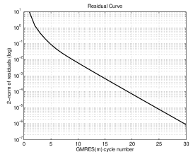
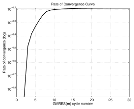
Geometrically, the theorem suggests that any residual curve of a restarted GMRES, applied to a system with a nonsingular normal matrix, is nonincreasing and concave up (Figure 1).

Refer to caption
Refer to caption
Fig. 1: Cycle–convergence of GMRES(5) applied to a 100–by –100 normal matrix.

From the proof of the Theorem 5 it is clear that, for a fixed $k$, the equality in (12) holds if and only if the vector $w_{k}$ (14) from the null space of the corresponding matrix $K^{H}\left(A^{H},r_{k}\right)$ is zero. In particular, when the restart parameter is chosen to be one less than the problem size, i.e. $m=n-1$, the matrix $K^{H}\left(A^{H},r_{k}\right)$ in (13) becomes an $n$–by–$n$ nonsingular matrix, hence with a zero null space, and thus the Inequality (12) is indeed an equality when $m=n-1$.

It turns out that the cycle–convergence of GMRES($n-1$), applied to the system (1) with a nonsingular normal matrix $A$, can be completely determined by norms of the two initial residual vectors $r_{0}$ and $r_{1}$.

Corollary 6 (The cycle–convergence of GMRES($n-1$)).

Given $\|r_{0}\|$ and $\|r_{1}\|$. Then, under assumptions of the Theorem 5, norms of the residual vectors $r_{k}$ at the end of each GMRES($n-1$) cycle obey the following formula

(16) $$\|r_{k+1}\|=\|r_{1}\|\left(\frac{\|r_{1}\|}{\|r_{0}\|}\right)^{k},\quad k=1,\dots,q-1.$$

Proof. The representation (14) of the residual vector $r_{k-1}$, for $m=n-1$, turns into

(17) $$r_{k-1}=\|r_{k}\|^{2}\left(K^{H}\left(A^{H},r_{k}\right)\right)^{-1}e_{1},$$

implying, by the proof of the Theorem 5, that the equality in (12) holds at each GMRES($n-1$) cycle. Thus,

$$\|r_{k+1}\|=\|r_{k}\|\frac{\|r_{k}\|}{\|r_{k-1}\|},\quad k=1,\dots,q-1.$$

We show (16) by induction in $k$. Using the formula above, it is easy to verify (16) for $\|r_{2}\|$ and $\|r_{3}\|$ ($k=1,2$). Let’s assume that for some $k$, $3\leq k\leq q-1$, $\|r_{k-1}\|$ and $\|r_{k}\|$ can also be computed by (16). Then

$\displaystyle\|r_{k+1}\|$ $\displaystyle=\|r_{k}\|\frac{\|r_{k}\|}{\|r_{k-1}\|}=\|r_{1}\|\left(\frac{\|r_{1}\|}{\|r_{0}\|}\right)^{k-1}\frac{\|r_{1}\|\left(\frac{\|r_{1}\|}{\|r_{0}\|}\right)^{k-1}}{\|r_{1}\|\left(\frac{\|r_{1}\|}{\|r_{0}\|}\right)^{k-2}}$
$\displaystyle=\|r_{1}\|\left(\frac{\|r_{1}\|}{\|r_{0}\|}\right)^{k-1}\left(\frac{\|r_{1}\|}{\|r_{0}\|}\right)=\|r_{1}\|\left(\frac{\|r_{1}\|}{\|r_{0}\|}\right)^{k}.$

Thus, (16) holds for all $k=1,\dots,q-1$. $\square$

Another observation in the proof of the Theorem 5 leads to a well known result due to Baker, Jessup and Manteuffel [1]. In this paper, the authors prove that, when GMRES($n-1$) is applied to a system with Hermitian or skew-Hermitian matrix, the residual vectors at the end of each restart cycle alternate direction in a cyclic fashion [1, Theorem 2]. In the following corollary we (slightly) refine this result by providing the exact expression for the constants $\alpha_{k}$ in [1, Theorem 2].

Corollary 7 (The alternating residuals).

Let $r_{k}$ be a sequence of nonzero residual vectors produced by GMRES($n-1$) applied to the system (1) with a nonsingular Hermitian or skew-Hermitian matrix $A\in\mathbb{C}^{n\times n}$. Then

(18) $$r_{k+1}=\alpha_{k}r_{k-1},\quad\alpha_{k}=\frac{\left\|r_{k+1}\right\|^{2}}{\left\|r_{k}\right\|^{2}}\in\left(0,1\right],\quad k=1,2,\dots,q-1.$$

Proof. For the case of a Hermitian matrix $A$, i.e. $A^{H}=A$, the proof follows directly from (17) and (7).

Let $A$ be skew-Hermitian, i.e. $A^{H}=-A$. Then, by (17) and (7),

$$r_{k-1}=\left(K^{H}\left(A^{H},r_{k}\right)\right)^{-1}e_{1}=\left(K^{H}\left(-A,r_{k}\right)\right)^{-1}e_{1}=\frac{\|r_{k}\|^{2}}{\|\hat{r}_{k+1}\|^{2}}\hat{r}_{k+1},$$

where $\hat{r}_{k+1}$ is the residual vector produced at the end of the cycle GMRES($-A$, $n-1$, $r_{k}$).

According to (3), the residual vectors $r_{k+1}$ and $\hat{r}_{k+1}$ at the end of the cycles GMRES($A$, $n-1$, $r_{k}$) and GMRES($-A$, $n-1$, $r_{k}$) are obtained by orthogonalizing $r_{k}$ against the Krylov residual subspaces $A\mathcal{K}_{n-1}\left(A,r_{k}\right)$ and $\left(-A\right)\mathcal{K}_{n-1}\left(-A,r_{k}\right)$ respectively. But $\left(-A\right)\mathcal{K}_{n-1}\left(-A,r_{k}\right)=A\mathcal{K}_{n-1}\left(A,r_{k}\right)$, hence $\hat{r}_{k+1}=r_{k+1}$. $\square$

4 Note on the departure from normality

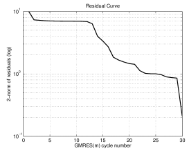
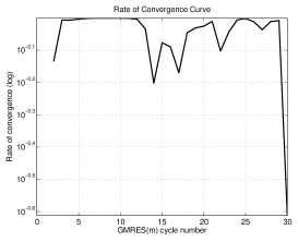
In general, for systems with nonnormal matrices, the cycle–convergence behavior of the restarted GMRES is not sublinear. In Figure 2, we take a nonnormal diagonalizable matrix for illustration purpose and one can observe the claim. Indeed, for nonnormal matrices, it has been observed the cycle–convergence of restarted GMRES can be superlinear [18].

In this concluding section we restrict our attention to the case of a diagonalizable matrix $A$,

(19) $$A=V\Lambda V^{-1},\quad A^{H}=V^{-H}\overline{\Lambda}V^{H}.$$

The analysis performed in Theorem 5 can be generalized for the case of a diagonalizable matrix ([16]), resulting in the inequality (15). However, as we depart from normality, Lemma 4 fails to hold and the norm of the residual vector $\hat{r}_{k+1}$ at the end of the cycle GMRES($A^{H}$, $m$, $r_{k}$) is no longer equal to the norm of the vector $r_{k+1}$ at the end of GMRES($A$, $m$, $r_{k}$). Moreover, since the eigenvectors of $A$ can be significantly changed by the Hermitian conjugation, as (19) suggests, the matrices $A$ and $A^{H}$ can have almost nothing in common, so that the norms of $\hat{r}_{k+1}$ and $r_{k+1}$ are, possibly, far from being equal. This gives a chance for breaking the sublinear convergence of GMRES($m$), provided that the subspace $A\mathcal{K}_{m}\left(A,r_{k}\right)$ results in a better approximation (3) of the vector $r_{k}$ than the subspace $A^{H}\mathcal{K}_{m}\left(A^{H},r_{k}\right)$.

It is natural to expect that the convergence of the restarted GMRES for “almost normal” matrices will be “almost sublinear”. We quantify this statement in the following lemma.

Refer to caption
Refer to caption
Fig. 2: Cycle–convergence of GMRES(5) applied to a 100–by–100 diagonalizable (nonnormal) matrix.
Lemma 8.

Let $r_{k}$ be a sequence of nonzero residual vectors produced by GMRES($m$) applied to the system (1) with a nonsingular diagonalizable (19) matrix $A\in\mathbb{C}^{n\times n}$, $1\leq m\leq n-1$. Then

(20) $$\frac{\|r_{k}\|}{\|r_{k-1}\|}\leq\frac{\alpha\left(\|r_{k+1}\|+\beta_{k}\right)}{\|r_{k}\|},\quad k=1,\dots,q-1,$$

where $\alpha=\frac{1}{\sigma_{min}^{2}(V)}$, $\beta_{k}=\|p_{k}(A)(I-VV^{H})r_{k}\|$, $p_{k}(z)$ is the polynomial constructed at the cycle GMRES($A$, $m$, $r_{k}$), and where $q$ is the total number of GMRES($m$) cycles. Note that as $V^{H}V\longrightarrow I$, $0<\alpha\longrightarrow 1$ and $0<\beta_{k}\longrightarrow 0$.

Proof. Consider the norm of the residual vector $\hat{r}_{k+1}$ at the end of the cycle GMRES($A^{H}$, $m$, $r_{k}$).

$$\|\hat{r}_{k+1}\|=\min_{\hat{p}\in\mathcal{P}_{m}}\|\hat{p}(A^{H})r_{k}\|\leq\|p(A^{H})r_{k}\|,$$

where $p(z)\in\mathcal{P}_{m}$ is any polynomial of degree at most $m$, such that $p(0)=1$. Then, using (19),

$\displaystyle\|\hat{r}_{k+1}\|$ $\displaystyle\leq$ $\displaystyle\|p(A^{H})r_{k}\|$
$\displaystyle=$ $\displaystyle\|V^{-H}p(\overline{\Lambda})V^{H}r_{k}\|$
$\displaystyle=$ $\displaystyle\|V^{-H}p(\overline{\Lambda})(V^{-1}V)V^{H}r_{k}\|$
$\displaystyle=$ $\displaystyle\|V^{-H}p(\overline{\Lambda})V^{-1}(VV^{H})r_{k}\|$
$\displaystyle=$ $\displaystyle\|V^{-H}p(\overline{\Lambda})V^{-1}(I-(I-VV^{H}))r_{k}\|$
$\displaystyle=$ $\displaystyle\|V^{-H}p(\overline{\Lambda})\left(V^{-1}r_{k}-V^{-1}(I-VV^{H})r_{k}\right)\|$
$\displaystyle\leq$ $\displaystyle\|V^{-H}\|\|p(\overline{\Lambda})\left(V^{-1}r_{k}-V^{-1}(I-VV^{H})r_{k}\right)\|.$

Note that

$$\|p(\overline{\Lambda})\left(V^{-1}r_{k}-V^{-1}(I-VV^{H})r_{k}\right)\|=\|\overline{p}(\Lambda)\left(V^{-1}r_{k}-V^{-1}(I-VV^{H})r_{k}\right)\|.$$

Thus,

$\displaystyle\|\hat{r}_{k+1}\|$ $\displaystyle\leq$ $\displaystyle\|V^{-H}\|\|\overline{p}(\Lambda)\left(V^{-1}r_{k}-V^{-1}(I-VV^{H})r_{k}\right)\|$
$\displaystyle=$ $\displaystyle\|V^{-H}\|\|(V^{-1}V)\overline{p}(\Lambda)\left(V^{-1}r_{k}-V^{-1}(I-VV^{H})r_{k}\right)\|$
$\displaystyle\leq$ $\displaystyle\|V^{-H}\|\|V^{-1}\|\|V\overline{p}(\Lambda)V^{-1}r_{k}-V\overline{p}(\Lambda)V^{-1}(I-VV^{H})r_{k}\|$
$\displaystyle=$ $\displaystyle\frac{1}{\sigma_{min}^{2}(V)}\|\overline{p}(V\Lambda V^{-1})r_{k}-\overline{p}(V\Lambda V^{-1})(I-VV^{H})r_{k}\|$
$\displaystyle\leq$ $\displaystyle\frac{1}{\sigma_{min}^{2}(V)}\left(\|\overline{p}(A)r_{k}\|+\|\overline{p}(A)(I-VV^{H})r_{k}\|\right),$

where $\sigma_{min}$ is the smallest singular values of $V$.

Since the last inequality holds for any polynomial $\overline{p}(z)\in\mathcal{P}_{m}$, it will also hold for $\overline{p}(z)=p_{k}(z)$, where $p_{k}(z)$ is the polynomial constructed at the cycle GMRES($A$, $m$, $r_{k}$). Hence,

$$\|\hat{r}_{k+1}\|\leq\frac{1}{\sigma_{min}^{2}(V)}\left(\|r_{k+1}\|+\|p_{k}(A)(I-VV^{H})r_{k}\|\right).$$

Setting $\alpha=\frac{1}{\sigma_{min}^{2}(V)}$, $\beta_{k}=\|p_{k}(A)(I-VV^{H})r_{k}\|$ and observing that $\alpha\longrightarrow 1$, $\beta_{k}\longrightarrow 0$ as $V^{H}V\longrightarrow I$, from (15), we obtain (20). $\square$

References

  • [1] A. H. Baker, E. R. Jessup, and T. Manteuffel, A Technique for Accelerating the Convergence of Restarted GMRES, SIAM Journal on Matrix Analysis and Applications, 26 (2005), pp. 962–984.
  • [2] S. Chandrasekaran and I. C. F. Ipsen, On the sensitivity of solution components in linear systems of equations, SIAM Journal on Matrix Analysis and Applications, 16 (1995), pp. 93–112.
  • [3] H. V. der Vorst and C.Vuik, The superlinear convergence behaviour of GMRES, Journal of Computational and Applied Mathematics, 48 (1993), pp. 327–341.
  • [4] M. Eiermann, Fields of values and iterative methods, Numerical Linear Algebra with Applications, 180 (1993), pp. 167–197.
  • [5] M. Embree, The Tortoise and the Hare Restart GMRES, SIAM Review, 45 (2003), pp. 259–266.
  • [6] J. Erhel, K. Burrage, and B. Pohl, Restarted GMRES preconditioned by deflation, Journal of Computational and Applied Mathematics, 69 (1996), pp. 303–318.
  • [7] A. Greenbaum, V. Pták, and Z. Strakoš, Any Nonincreasing Convergence Curve is Possible for GMRES, SIAM Journal on Matrix Analysis and Applications, 17 (1996), pp. 465–469.
  • [8] A. Greenbaum and Z. Strakoš, Matrices that generate the same Krylov residual spaces, in: Recent Advances in Iterative Methods, Springer, 1994, pp. 95–118.
  • [9] A. Greenbaum and L. N. Trefethen, GMRES/CR and Arnoldi/Lanczos as matrix approximation problems, SIAM Journal on Scientific Computing, 15 (1994), pp. 359–368.
  • [10] I. C. Ipsen, Expressions and bounds for the GMRES residual, BIT, 40 (2000), pp. 524–535.
  • [11] W. Joubert, On the convergence behavior of the restarted GMRES algorithm for solving nonsymmetric linear systems, Numerical Linear Algebra with Applications, 1 (1994), pp. 427–447.
  • [12] Y. Saad and M. H. Schultz, GMRES: A Generalized Minimal Residual Algorithm for Solving Nonsymmetric Linear Systems, SIAM Journal on Scientific and Statistical Computing, 7 (1986), pp. 856–869.
  • [13] G. W. Stewart, Collinearity and least squares regression, Statistical Science, 2 (1987), pp. 68–84.
  • [14] K.-C. Toh, GMRES vs. Ideal GMRES, SIAM Journal on Matrix Analysis and Applications, 18 (1997), pp. 30–36.
  • [15] L. N. Trefethen, Approximation theory and numerical linear algebra, in Algorithms for Approximation II, Chapman and Hall, London, U.K., 1990.
  • [16] I. Zavorin, Spectral Factorization of the Krylov matrix and convergence of GMRES, tech. rep., University of Maryland Computer Science Department, http://hdl.handle.net/1903/1168, 2002.
  • [17] I. Zavorin, D. P. O’Leary, and H. Elman, Complete stagnation of GMRES, Linear Algebra and its Applications, 367 (2003), pp. 165–183.
  • [18] B. Zhong and R. B. Morgan, Complementary Cycles of Restarted Gmres. Numerical Linear Algebra with Applications, to appear.