Maximally Localized Wannier Functions within the FLAPW formalism

Abstract

We report on the implementation of the Wannier Functions (WFs) formalism within the full-potential linearized augmented plane wave method (FLAPW), suitable for bulk, film and one-dimensional geometries. The details of the implementation, as well as results for the metallic SrVO₃, ferroelectric BaTiO₃ grown on SrTiO₃, covalently bonded graphene and a one-dimensional Pt-chain are given. We discuss the effect of spin-orbit coupling on the Wannier Functions for the cases of SrVO₃ and platinum. The dependency of the WFs on the choice of the localized trial orbitals as well as the difference between the maximally localized and ”first-guess” WFs are discussed. Our results on SrVO₃ and BaTiO₃, e.g. the ferroelectric polarization of BaTiO₃, are compared to results published elsewhere and found to be in excellent agreement.

I Introduction

Commonly, the electronic structure of periodic solids is described in terms of Bloch functions (BFs), which are eigenfunctions of both the Hamiltonian and lattice translation operators. Due to their delocalized nature BFs are difficult to visualize and hence do not offer a very intuitive picture of the underlying physics. Furthermore, BFs do not provide an efficient framework for the study of local correlations. An alternative approach to electronic structure that does not exhibit these weaknesses is provided by maximally localized Wannier functions (MLWFs). Related to the BFs via a unitary transformation, MLWFs constitute a mathematically equivalent concept for the study of electronic structure. They are well localized in real space and in contrast to the complex BFs purely real rea . Therefore, it is easy to visualize them and to gain physical insight e.g. into the bonding properties of the system under study by extracting characteristic parameters such as the MLWFs’ centers, spreads, and hopping integrals as well as by analyzing their shapes.

Wannier functions (WFs) were first introduced by Wannier in 1937 Wannier (1937) as the Fourier transforms of BFs. Similar to a $\delta$-function, which is the Fourier transform of a plane wave, WFs are localized in real space while the BFs are not. However, BFs are only determined up to an arbitrary phase factor, and hence the definition of WFs as Fourier transforms of BFs does not specify the WFs uniquely. As the localization properties of the WFs depend strongly on the phase factors of the BFs, the Wannier function approach experienced little enthusiasm until very recently, after methods for the calculation of WFs with optimal localization properties had been developed. One of these new techniques for the construction of localized WFs is based on the N-th order muffin-tin-orbital (NMTO) method. Andersen and Saha-Dasgupta (2000); Pavarini et al. (2005); Zurek et al. (2005) Another method performs at each $k$-point a unitary transformation among the BFs belonging to different bands yielding a new set of functions, the Fourier transforms of which are the MLWFs. Marzari and Vanderbilt (1997) The MLWFs approach is not limited to insulators but is also capable of providing well localized orbitals for metals. Souza et al. (2001) Only the latter technique is considered in this work.

Sheding new light on otherwise hard to calculate properties of materials, nowadays MLWFs have almost reached the popularity of BFs, and using both allows to achieve a rich diversity in understanding, originating from revealing both itinerant and localized aspects of electrons in periodic potentials. For example, a modern theory of polarization King-Smith and Vanderbilt (1993); Vanderbilt and King-Smith (1993); Marzari and Vanderbilt (1998); Resta (1994); Wu et al. (2006) is based on the displacements of the centers of the MLWFs. The orbital polarization may be expressed in terms of MLWFs. Thonhauser et al. (2005); Ceresoli et al. (2006) Studying the MLWFs for disordered systems yields a transparent description of bonding properties. Silvestrelli et al. (1998) MLWFs provide a minimal basis set that allows for efficient computations of the quantum transport of electrons through nanostructures and molecules. Thygesen and Jacobsen (2005); Calzolari et al. (2004) Within the research area of strongly correlated electrons MLWFs are becoming the preferred basis for studying the local correlations. Pavarini et al. (2004); Anisimov et al. (2005); Lechermann et al. (2006)

The MLWFs-induced burst in studying the properties of materials which are hard to probe on the basis of traditional band theory is very recent and many subtle aspects, such as magnetism, various spin-orbit coupling and non-collinearity-driven effects are still to be put on the MLWFs footing. In this respect the precision of the computational electronic structure method used for the construction of the MLWFs might play a very important role, as sophisticated details of the electronic structure and tiny energy scales are involved. In particular in magnetism, the choice of the appropriate ab initio method plays a crucial role. From this point of view it is common consensus that the full-potential linearized augmented plane wave method (FLAPW) is one of the most precise electronic structure methods used today. Ab-initio MLWFs have already been calculated within the FLAPW framework for MnO Posternak et al. (2002) and TiO₂. Cangiani et al. (2004); Posternak et al. (2006)

In the present paper we report in detail on the implementation of MLWFs within the FLAPW method as implemented in the FLEUR fle code. The current implementation allows a fast computation of MLWFs for a large variety of materials and complex geometries, including bulk, film Krakauer et al. (1979) and truly one-dimensional geometrical setups. Mokrousov et al. (2005) To verify our implementation we apply the method to four different systems, two different perovskite systems, SrVO₃ and BaTiO₃, one metallic and one ferroelectric, graphene, a covalently bonded material, and a one-dimensional Pt-chain. This article is structured as follows: We start in section II with a short outline of MLWFs and their construction procedure, defining the quantities required from the first-principles calculation based on the density functional theory (DFT) by the maximal localization algorithm. First-guess WFs – originally devised as a starting point for the MLWF-algorithm, but widely used as a suitable alternative to the MLWFs – are introduced. Then, the details of our FLAPW implementation are described. In Section III we apply the formalism to SrVO₃, BaTiO₃, graphene and a one-dimensional Pt-chain. We discuss the effects of spin-orbit coupling on the MLWFs for SrVO₃ and the Pt-chain. We compare our results on SrVO₃ and BaTiO₃ with theoretical and experimental data, respectively, and find excellent agreement. Finally we close this work with conclusions in Section IV.

II Method

II.1 Maximally localized Wannier functions

For an isolated band, i.e. a band that does not become degenerate with other bands at any $k$-point, with corresponding BFs $|\psi_{{\bf{k}}}\rangle$, the definition of WFs as Fourier transforms of BFs leads to the following expression:

$$|W_{{\bf{R}}}\rangle=\frac{1}{N}\sum_{{\bf{k}}}e^{-i{\bf{k}}\cdot{\bf{R}}}|\psi_{{\bf{k}}}\rangle,$$ (1)

where ${\bf{R}}$ is a direct lattice vector, which specifies the unit cell the WF belongs to, and the Brillouin zone is represented by a uniform mesh of $N$ $k$-points. The $|\psi_{{\bf{k}}}\rangle$ are normalized with respect to the unit cell, while the $|W_{{\bf{R}}}\rangle$ constitute an orthonormal basis set with respect to the volume of $N$ unit cells.

However, Eq. (1) does not define the WFs uniquely: The BFs are determined only up to a phase factor – hence, for a given set of BFs and a general $k$-point dependent phase $\phi({\bf{k}})$,

$$|W_{{\bf{R}}}\rangle^{\prime}=\frac{1}{N}\sum_{{\bf{k}}}e^{-i{\bf{k}}\cdot{\bf{R}}}e^{i\phi({\bf{k}})}|\psi_{{\bf{k}}}\rangle$$ (2)

equally constitute a set of WFs. For their use in practice, it is desirable to have WFs that decay exponentially in real space, exhibit the symmetry properties of the system studied, and are real- rather than complex-valued functions rea . For the one-dimensional Schrödinger equation and an isolated single energy band, Kohn Kohn (1959) has shown that there exists only one WF which is real rea , falls off exponentially with distance and has maximal symmetry. WFs with maximal spatial localization Marzari and Vanderbilt (1997) (MLWFs) fulfill these requirements of real-valuedness rea , optimal decay properties and maximal symmetry. The constraint of maximal localization eliminates the nonuniqueness of WFs and determines $\phi({\bf{k}})$ up to a constant.

In the general case, energy bands cross or are degenerate at certain $k$-points, making it necessary to consider a group of bands. This increases the freedom in defining WFs further, as now bands may be mixed at each $k$-point via the transformation $U_{mn}^{({\bf{k}})}$:

$$|W_{{\bf{R}}n}\rangle=\frac{1}{N}\sum_{{\bf{k}}}e^{-i{\bf{k}}\cdot{\bf{R}}}\sum_{m}U_{mn}^{({\bf{k}})}|\psi_{{\bf{k}}m}\rangle,$$ (3)

where the BF has a band index $m$, the WF an orbital index $n$, and the number of bands – which may depend on the $k$-point – has to be larger than or equal to the number of WFs that are supposed to be extracted. Imposing the constraint of maximal spatial localization on the WFs determines the set of $U_{mn}^{({\bf{k}})}$-matrices up to a common global phase. Marzari and Vanderbilt (1997); Souza et al. (2001) In case the number of bands is equal to the number of WFs, the $U_{mn}^{({\bf{k}})}$ matrices are unitary. This situation usually occurs when an isolated group of bands may efficiently be chosen for the system under study. In the more general case of entangled energy bands, Souza et al. (2001) however, the number of bands is $k$-point dependent and $U_{mn}^{({\bf{k}})}$ no longer unitary.

II.2 Maximal localization procedure

Requiring the spread of the WFs to be minimal imposes the constraint of maximal spatial localization. For the spread of the WFs the sum of the second moments,

$$\Omega=\sum_{n}[\langle{\bf{x}}^{2}\rangle_{n}-(\langle{\bf{x}}\rangle_{n})^{2}],$$ (4)

is used, where $\langle\rangle_{n}$ denotes the expectation value with respect to the Wannier orbital $|W_{{\bf{0}}n}\rangle$ and the sum includes all WFs formed from the composite group of bands. Minimization of the spread yields the set of optimal $U_{mn}^{({\bf{k}})}$-matrices.

An efficient algorithm for the minimization of the spread Eq. (4) has been given by Marzari and Vanderbilt first for isolated groups of bands, Marzari and Vanderbilt (1997) and later on generalized for the case of entangled energy bands. Souza et al. (2001) The corresponding computer code is publicly available MLW and was used in this work. Two quantities are required as input by this computational method and have to be provided by the first-principles calculation: First, the projections $A_{mn}^{({\bf{k}})}=\langle\psi_{{\bf{k}}m}|g_{n}\rangle$ of localized orbitals $|g_{n}\rangle$ onto the BFs are needed to construct a starting point for the iterative optimization of the MLWFs. Second, the overlaps between the lattice periodic parts $u_{{\bf{k}}m}({\bf{x}})=e^{-i{\bf{k}}\cdot{\bf{x}}}\psi_{{\bf{k}}m}({\bf{x}})$ of the BFs at nearest-neighbor $k$-points ${\bf{k}}$ and ${\bf{k}}+{\bf{b}}$, $M_{mn}^{({\bf{k}},{\bf{b}})}=\langle u_{{\bf{k}}m}|u_{{\bf{k}}+{\bf{b}},n}\rangle$, are necessary to evaluate the relevant observables Marzari and Vanderbilt (1997):

$$\langle{\bf{x}}\rangle_{n}=-\frac{1}{N}\sum_{{\bf{k}},{\bf{b}}}w_{{\bf{b}}}\,{\bf{b}}\,\Im\ln\tilde{M}_{nn}^{({\bf{k}},{\bf{b}})}$$ (5)

and

$$\langle{\bf{x}}^{2}\rangle_{n}=\frac{1}{N}\sum_{{\bf{k}},{\bf{b}}}w_{{\bf{b}}}\,[1-|\tilde{M}_{nn}^{({\bf{k}},{\bf{b}})}|^{2}+(\Im\ln\tilde{M}_{nn}^{({\bf{k}},{\bf{b}})})^{2}],$$ (6)

where $w_{{\bf{b}}}$ is a weight associated with ${\bf{b}}$, and

$$\tilde{M}_{mn}^{({\bf{k}},{\bf{b}})}=\sum_{m_{1}}\sum_{m_{2}}(U_{m_{1}m}^{({\bf{k}})})^{*}U_{m_{2}n}^{({\bf{k}}+{\bf{b}})}M_{m_{1}m_{2}}^{({\bf{k}},{\bf{b}})}$$ (7)

evolves during the minimization process due to the iterative refinement of the $U_{mn}^{({\bf{k}})}$. The relations Eqns. (5, 6) are valid for uniform $k$-point grids, while in the continuum-limit the $k$-space expressions for the matrix elements of the position operator are given by Marzari and Vanderbilt (1997)

$$\langle W_{{\bf{R}}n}|{\bf{x}}|W_{{\bf{0}}m}\rangle=i\frac{V}{2\pi^{3}}\int d^{3}ke^{i{\bf{k}}\cdot{\bf{R}}}\langle\tilde{u}_{{\bf{k}}n}|\nabla_{{\bf{k}}}|\tilde{u}_{{\bf{k}}m}\rangle$$ (8)

and

$$\langle W_{{\bf{R}}n}|{\bf{x}}^{2}|W_{{\bf{0}}m}\rangle=-\frac{V}{2\pi^{3}}\int d^{3}ke^{i{\bf{k}}\cdot{\bf{R}}}\langle\tilde{u}_{{\bf{k}}n}|\nabla^{2}_{{\bf{k}}}|\tilde{u}_{{\bf{k}}m}\rangle.$$ (9)

Replacing the gradient $\nabla_{{\bf{k}}}$ by finite-difference expressions valid on a uniform $k$-point mesh, one obtains the weights $w_{{\bf{b}}}$ in Eqns. (5, 6). Through Eqns. (5, 6, 7) the spread $\Omega$ in Eq. (4) may be expressed in terms of and be minimized with respect to the $U_{mn}^{({\bf{k}})}$-matrices.

II.3 First-guess Wannier functions

The iterative optimization process requires as a starting point first guesses for the MLWFs. In order to construct these, one projects localized orbitals $|g_{n}\rangle$ onto the BF-subspace:

$$|\phi_{{\bf{k}}n}\rangle=\sum_{m}|\psi_{{\bf{k}}m}\rangle\langle\psi_{{\bf{k}}m}|g_{n}\rangle=\sum_{m}A^{({\bf{k}})}_{mn}\,|\psi_{{\bf{k}}m}\rangle.$$ (10)

As the first-guess WFs are supposed to constitute an orthonormal basis set, the $|\phi_{{\bf{k}}n}\rangle$ are orthonormalized via the overlap matrix $S_{mn}^{({\bf{k}})}=\langle\phi_{{\bf{k}}m}|\phi_{{\bf{k}}n}\rangle$

$$|\tilde{\psi}_{{\bf{k}}n}\rangle=\sum_{m}((S^{({\bf{k}})})^{-\frac{1}{2}})_{mn}|\phi_{{\bf{k}}m}\rangle,$$ (11)

before the WFs are calculated from them

$$|W_{{\bf{R}}n}\rangle=\frac{1}{N}\sum_{{\bf{k}}}e^{-i{\bf{k}}\cdot{\bf{R}}}|\tilde{\psi}_{{\bf{k}}n}\rangle.$$ (12)

While the first-guess WFs are dependent on the choice of localized orbitals $|g_{n}\rangle$ they converge to the one and only one set of MLWFs in the course of the minimization procedure.

Although the first-guess WFs of Eq. (12) are not unique they agree well with the MLWFs in many cases. Examples where there is substantial difference between first-guess WFs and MLWFs include systems where the centers of the Wannier orbitals do not coincide with the centers of the atoms. If for the system under study the first-guess WFs are already satisfactory, one may skip the localization procedure and take Eq. (12) as the final result. Computing WFs in such a way requires much less time, as the $M_{mn}^{({\bf{k}},{\bf{b}})}$ matrix elements do not have to be calculated and the minimization of the spread functional is not performed. First-guess WFs have been successfully applied to SrVO₃, Anisimov et al. (2005) V₂O₃ Anisimov et al. (2005) and NiO, Ren et al. (2006) for example.

II.4 Calculation of $M_{mn}^{({\bf{k}},{\bf{b}})}$ within the FLAPW formalism

For the calculation of MLWFs the most important quantity is the $M_{mn}^{({\bf{k}},{\bf{b}})}$ matrix, which – according to Eqns. (5, 6) – contains all information needed to determine spreads and centers. With the lattice periodic part $u_{{\bf{k}}m}({\bf{x}})$ being related to its BF by $u_{{\bf{k}}m}({\bf{x}})=e^{-i{\bf{k}}\cdot{\bf{x}}}\psi_{{\bf{k}}m}({\bf{x}})$, the $M_{mn}^{({\bf{k}},{\bf{b}})}$ matrix elements assume the form

$$M_{mn}^{({\bf{k}},{\bf{b}})}=\int e^{-i{\bf{b}}\cdot{\bf{x}}}(\psi_{{\bf{k}}m}({\bf{x}}))^{*}\psi_{[{\bf{k}}+{\bf{b}}],n}({\bf{x}})\,d^{3}x.$$ (13)

By $[{\bf{k}}]$ we denote the wave vector obtained from ${\bf{k}}$ by subtracting the reciprocal lattice vector that moves ${\bf{k}}$ into the first Brillouin zone, according to $[{\bf{k}}]={\bf{k}}-\mathbf{G}({\bf{k}})$.

Within FLAPW, Hamann (1979); Wimmer et al. (1981) space is partitioned into the muffin-tin (MT) spheres centered around atoms $\mu$ and the interstitial (INT) region. Consequently, $M_{mn}^{({\bf{k}},{\bf{b}})}$ has contributions from both,

$$M_{mn}^{({\bf{k}},{\bf{b}})}=M_{mn}^{({\bf{k}},{\bf{b}})}|_{\text{INT}}+\sum_{\mu}M_{mn}^{({\bf{k}},{\bf{b}})}|_{\text{MT}^{\mu}},$$ (14)

which will be discussed separately in the following. The treatment of the vacuum regions occurring in film and one-dimensional setups is discussed in the appendices A and B, respectively.

Inside the muffin-tin, the BF is expanded into spherical harmonics, radial basis functions $u_{l}$, which are solutions of the scalar relativistic equation at band-averaged energies, and the energy derivatives $\dot{u}_{l}$ of the $u_{l}$:

$$\psi_{{\bf{k}}m}({\bf{x}})|_{\text{MT}^{\mu}}$$ (15)

$$=\sum_{L}(A^{\mu}_{L,m}({\bf{k}})u_{l}^{\mu}(r)+B^{\mu}_{L,m}({\bf{k}})\dot{u}_{l}^{\mu}(r))Y_{L}(\hat{{\bf{r}}}),$$

where atom $\mu$ is located at ${\bm{\tau}}_{\mu}$ and ${\bf{r}}={\bf{x}}-{\bm{\tau}}_{\mu}$. Here, $m$ is the band-index and $L=(l,l_{z})$ stands for the angular momentum quantum numbers $l$ and $l_{z}$. The case where the lapw basis is supplemented with local orbitals is treated in the appendix C. Using the Rayleigh plane wave expansion

$$e^{-i{\bf{b}}\cdot{\bf{x}}}=4\pi e^{-i{\bf{b}}\cdot{\bm{\tau}}_{\mu}}\sum_{L}(-1)^{l}i^{l}j_{l}(rb)Y_{L}(\hat{{\bf{b}}})Y_{L}^{*}(\hat{{\bf{r}}}),$$ (16)

the contribution $M_{mn}^{({\bf{k}},{\bf{b}})}|_{\text{MT}^{\mu}}$ of the muffin-tin region of atom $\mu$ to the $M_{mn}^{({\bf{k}},{\bf{b}})}$ matrix reads:

$$M_{mn}^{({\bf{k}},{\bf{b}})}|_{\text{MT}^{\mu}}=4\pi e^{-i{\bf{b}}\cdot{\bm{\tau}}_{\mu}}$$ (17)

$$\times\sum_{L,L^{\prime}}(( A^{\mu}_{L,m}({\bf{k}}))^{*}A^{\mu}_{L^{\prime},n}([{\bf{k+b}}])t_{11}^{\mu}({\bf{b}},L,L^{\prime})$$

$$+( A^{\mu}_{L,m}({\bf{k}}))^{*}B^{\mu}_{L^{\prime},n}([{\bf{k+b}}])t_{12}^{\mu}({\bf{b}},L,L^{\prime})$$

$$+( B^{\mu}_{L,m}({\bf{k}}))^{*}A^{\mu}_{L^{\prime},n}([{\bf{k+b}}])t_{21}^{\mu}({\bf{b}},L,L^{\prime})$$

$$+( B^{\mu}_{L,m}({\bf{k}}))^{*}B^{\mu}_{L^{\prime},n}([{\bf{k+b}}])t_{22}^{\mu}({\bf{b}},L,L^{\prime})).$$

The matrix elements $t_{11}^{\mu}({\bf{b}},L^{\prime\prime},L)$ and $t_{12}^{\mu}({\bf{b}},L^{\prime\prime},L)$ are given by the sums over radial integrals

$$t_{11}^{\mu}({\bf{b}},L^{\prime\prime},L)$$ (18)

$$=\sum_{L^{\prime}}\mathsf{G}_{ll^{\prime}l^{\prime\prime}}^{mm^{\prime}m^{\prime\prime}}(\hat{{\bf{b}}}) \int r^{2}j_{l^{\prime}}(rb)u_{l}^{\mu}(r)u_{l^{\prime\prime}}^{\mu}(r)d\,r,$$

$$t_{12}^{\mu}({\bf{b}},L^{\prime\prime},L)$$

$$=\sum_{L^{\prime}}\mathsf{G}_{ll^{\prime}l^{\prime\prime}}^{mm^{\prime}m^{\prime\prime}}(\hat{{\bf{b}}}) \int r^{2}j_{l^{\prime}}(rb)\dot{u}_{l}^{\mu}(r)u_{l^{\prime\prime}}^{\mu}(r)d\,r,$$

and analogously for $t_{21}^{\mu}$ and $t_{22}^{\mu}$, where

$$\mathsf{G}_{ll^{\prime}l^{\prime\prime}}^{mm^{\prime}m^{\prime\prime}}(\hat{{\bf{b}}})=G_{ll^{\prime}l^{\prime\prime}}^{mm^{\prime}m^{\prime\prime}}i^{l^{\prime}}(-1)^{l^{\prime}}Y_{L^{\prime}}(\hat{{\bf{b}}}),$$ (19)

with the Gaunt coefficients

$$G_{ll^{\prime}l^{\prime\prime}}^{mm^{\prime}m^{\prime\prime}}=\int Y_{lm}(\hat{{\bf{r}}})Y^{*}_{l^{\prime}m^{\prime}}(\hat{{\bf{r}}})Y^{*}_{l^{\prime\prime}m^{\prime\prime}}(\hat{{\bf{r}}})\,d\Omega.$$ (20)

The quantities defined in Eq. (18) depend on the vectors ${\bf{b}}$ joining a given $k$-point to its nearest neighbors. As a uniform $k$-mesh is used the set of ${\bf{b}}$ vectors and hence also the integrals defined in Eq. (18) are independent of the $k$-point. Thus, the quantities Eq. (18) have to be calculated only once.

Employing the expansion of the BF in the interstitial region

$$\psi_{{\bf{k}}m}({\bf{x}})=\frac{1}{\sqrt{V}}\sum_{{\bf{G}}}c_{{\bf{k}}m}({\bf{G}})e^{i({\bf{k}}+{\bf{G}})\cdot{\bf{x}}},$$ (21)

the INT contribution to the $M_{mn}^{({\bf{k}},{\bf{b}})}$ matrix is deduced:

$$\begin{split}M_{mn}^{({\bf{k}},{\bf{b}})}|_{\text{INT}}=\frac{1}{V}\sum_{{\bf{G}},{\bf{G^{\prime}}}}(c_{{\bf{k}},m}({\bf{G}}))^{*}c_{[{\bf{k}}+{\bf{b}}],n}({\bf{G^{\prime}}})\\ \times\int_{\text{INT}}e^{i([{\bf{k}}+{\bf{b}}]+{\bf{G^{\prime}}})\cdot{\bf{x}}}\,e^{-i({\bf{k}}+{\bf{G}})\cdot{\bf{x}}}\,e^{-i{\bf{b}}\cdot{\bf{x}}}\,d^{3}x,\end{split}$$ (22)

where the integration stretches over the interstitial only. Introducing the step function $\Theta({\bf{x}})$, that cuts out the muffin tins, and its Fourier transform $\Theta_{{\bf{G}}}$, Eq. (22) can be cast into the final form

$$M_{mn}^{({\bf{k}},{\bf{b}})}|_{\text{INT}}$$ (23)

$$=\sum_{{\bf{G}},{\bf{G^{\prime}}}}(c_{{\bf{k}},m}({\bf{G}}))^{*}c_{[{\bf{k}}+{\bf{b}}],n}({\bf{G^{\prime}}})\Theta_{{\bf{G}}({\bf{k}}+{\bf{b}})+{\bf{G}}-{\bf{G^{\prime}}}},$$

where ${\bf{G}}({\bf{k}}+{\bf{b}})$ denotes the reciprocal space vector that moves $({\bf{k}}+{\bf{b}})$ into the first Brillouin zone, $[{\bf{k}}+{\bf{b}}]={\bf{k}}+{\bf{b}}-{\bf{G}}({\bf{k}}+{\bf{b}})$.

II.5 Calculation of $A_{mn}^{({\bf{k}})}$ within the FLAPW formalism

For the localized orbitals $|g_{n}\rangle$ required to determine the first-guess WFs, we mostly use functions that are zero everywhere in space except in the muffin-tin sphere of that atom, to which the resulting WF is attributed in this sense. In practice, this works not only for WFs that are atom-centered but also for bond-centered ones. Thus, $g_{n}({\bf{x}})$ is given by

$$g_{n}({\bf{x}})=\sum_{L}c_{n,L}\tilde{u}_{l}(r)Y_{L}(\hat{{\bf{r}}}),$$ (24)

where ${\bf{r}}={\bf{x}}-{\bm{\tau}}_{\mu}$ is the position relative to the center of the atom, to which the first-guess WF is attributed, and the coefficients $c_{n,L}$ control the angular distribution of $g_{n}({\bf{x}})$. For the radial part $\tilde{u}_{l}(r)$ of the localized orbital we use the solution $u_{l}^{\mu}(r)$ of the radial scalar relativistic equation for the actual potential obtained from the first-principles calculation at an energy corresponding to the bands from which the WF is constructed. It is also possible to use Gaussians, Marzari and Vanderbilt (1997) or the radial parts of hydrogenic wave functions for $\tilde{u}_{l}(r)$. Where angular momentum is concerned in Eq. (24), contributions of different angular momenta have to be summed in the general case to allow the definition of hybrids such as $sp^{3}$ orbitals, while there is only an $l=2$ contribution for WFs corresponding to $d$ orbitals, for example.

For a general radial part $\tilde{u}_{l}(r)$ the projection of the localized orbital $|g_{n}\rangle$ onto the BF is given by

$$\begin{array}[]{cc}A_{mn}^{({\bf{k}})}=\displaystyle\sum_{L}c_{n,L}[(a_{L,m}^{\mu}({\bf{k}}))^{*}\int u_{l}^{\mu}(r)\tilde{u}_{l}(r)r^{2}dr\\ \displaystyle+(b_{L,m}^{\mu}({\bf{k}}))^{*}\int\dot{u}_{l}^{\mu}(r)\tilde{u}_{l}(r)r^{2}dr],\end{array}$$ (25)

where the expansion of the BF given in Eq. (15) was used. Choosing $\tilde{u}_{l}(r)=u_{l}^{\mu}(r)$ Eq. (25) simplifies as follows:

$$A_{mn}^{({\bf{k}})}=\langle\psi_{{\bf{k}}m}|g_{n}\rangle=\sum_{L}c_{n,L}(a_{L,m}^{\mu}({\bf{k}}))^{*}.$$ (26)

In order to construct better first guesses for bond-centered WFs $|g_{n}\rangle$ may also be constructed as a linear combination of two localized orbitals - one orbital for each atom participating in the bond. Calculating the WFs for graphene in the next section we proceeded this way.

II.6 Wannier Representation of the Hamiltonian

Formulating the Hamiltonian in terms of WFs is a particularly useful starting point when effects of correlation Lechermann et al. (2006); Ren et al. (2006); Anisimov et al. (2005) are studied by DMFT. Furthermore, the hopping integrals – along with the MLWFs’ spreads, centers and shapes – provide intuitive insight into the electronic structure.

Written in terms of BFs the Hamiltonian $\hat{H}$ assumes the diagonal form

$$\hat{H}=\frac{1}{N}\sum_{{\bf{k}},n}\epsilon_{n}({\bf{k}})|\psi_{{\bf{k}}n}\rangle\langle\psi_{{\bf{k}}n}|,$$ (27)

where $\epsilon_{n}({\bf{k}})$ stand for the eigenvalues of $\hat{H}$. If the number of bands is equal to the number of MLWFs extracted the $U_{mn}^{({\bf{k}})}$-matrices in Eq. (3) are unitary. In this case we arrive at the equivalent form of the Hamiltonian

$$\hat{H}=\sum_{{\bf{R}}_{1}m}\sum_{{\bf{R}}_{2}m^{\prime}}H_{m,m^{\prime}}({\bf{R}}_{1}-{\bf{R}}_{2})|W_{{\bf{R}}_{1}m}\rangle\langle W_{{\bf{R}}_{2}m^{\prime}}|,$$ (28)

where

$$\begin{array}[]{cc}H_{m,m^{\prime}}({\bf{R}}_{1}-{\bf{R}}_{2})\\[5.69046pt] =\displaystyle\frac{1}{N}\sum_{{\bf{k}}n}\epsilon_{n}({\bf{k}})\langle W_{{\bf{R}}_{1}m}|\psi_{{\bf{k}}n}\rangle\langle\psi_{{\bf{k}}n}|W_{{\bf{R}}_{2}m^{\prime}}\rangle\\[5.69046pt] =\displaystyle\frac{1}{N}\sum_{{\bf{k}}n}\epsilon_{n}({\bf{k}})e^{i{\bf{k}}\cdot({\bf{R}}_{1}-{\bf{R}}_{2})}\left(U^{({\bf{k}})}_{nm}\right)^{*}U_{nm^{\prime}}^{({\bf{k}})}.\end{array}$$ (29)

The hopping integrals $H_{m,m^{\prime}}({\bf{R}}_{1}-{\bf{R}}_{2})$ quantify the hopping of electrons from Wannier orbital $|W_{{\bf{R}}_{2}m^{\prime}}\rangle$ into Wannier orbital $|W_{{\bf{R}}_{1}m}\rangle$.

II.7 Spin-orbit coupling

In the case of spin-orbit coupling Eq. (13) assumes the form

$$M_{mn}^{{\bf{k}},{\bf{b}}}=\sum_{\sigma}\int e^{-i{\bf{b}}\cdot{\bf{x}}}(\psi_{{\bf{k}}m\sigma}({\bf{x}}))^{*}\psi_{[{\bf{k}}+{\bf{b}}],n\sigma}({\bf{x}})d^{3}x,$$ (30)

where $\psi_{{\bf{k}}m\sigma}({\bf{x}})$ is the BF with lattice vector ${\bf{k}}$, band index $n$, and spin index $\sigma$. The spin index $\sigma$ refers to the eigenstates of the projection of the spin-operator onto the spin-quantization axis. Likewise Eq. (25) has to be changed into

$$A_{mn}^{({\bf{k}})}= \sum_{L}\sum_{\sigma}c_{nL\sigma}$$ (31)

$$\times[( a_{Lm\sigma}^{\mu}({\bf{k}}))^{*}\int u_{l,\sigma}^{\mu}(r)\tilde{u}_{l,\sigma}(r)r^{2}dr$$

$$+( b_{Lm\sigma}^{\mu}({\bf{k}}))^{*}\int\dot{u}_{l,\sigma}^{\mu}(r)\tilde{u}_{l,\sigma}(r)r^{2}dr].$$

In the regime from weak to modest spin-orbit coupling it is reasonable to choose the localized orbitals $|g_{n}\rangle$ to be eigenstates of the projection of the spin-operator onto the spin-quantization axis. This means that for given $n$ $c_{nL\sigma}$ may differ from zero only for one spin component $\sigma$.

Eq. (28) remains valid in the case of spin-orbit coupling, but the matrix elements $H_{m,m^{\prime}}({\bf{R}}_{1}-{\bf{R}}_{2})$ in Eq. (28) correspond to hopping between spinor-valued Wannier orbitals then, where the two spin-components are given by

$$|W_{{\bf{R}}m\sigma}\rangle=|\sigma\rangle\langle\sigma|W_{{\bf{R}}m}\rangle,\,\sigma=\uparrow,\downarrow.$$ (32)

Alternatively, the hopping matrix elements may be decomposed according to the spin-channels:

$$H_{mm^{\prime}}^{\sigma\sigma^{\prime}}({\bf{R}}_{1}-{\bf{R}}_{2})$$ (33)

$$=\frac{1}{N}\sum_{{\bf{k}}n}\epsilon_{n}({\bf{k}})\langle W_{{\bf{R}}_{1}m\sigma}|\Psi_{{\bf{k}}n}\rangle\langle\Psi_{{\bf{k}}n}|W_{{\bf{R}}_{2}m^{\prime}\sigma^{\prime}}\rangle$$

$$=\frac{1}{N}\sum_{{\bf{k}}n}\sum_{n^{\prime}n^{\prime\prime}}\epsilon_{n}({\bf{k}})e^{i{\bf{k}}\cdot({\bf{R}}_{1}-{\bf{R}}_{2})}$$

$$\times(U_{n^{\prime\prime}m}^{({\bf{k}})})^{*}O_{n^{\prime\prime}n\sigma}^{({\bf{k}})}O_{nn^{\prime}\sigma^{\prime}}^{({\bf{k}})}U_{n^{\prime}m^{\prime}}^{({\bf{k}})},$$

where the overlap $\langle\Psi_{{\bf{k}}n\sigma}|\Psi_{{\bf{k}}n^{\prime}\sigma}\rangle$ is denoted $O_{nn^{\prime}\sigma}^{({\bf{k}})}$. The corresponding real-space representation of the Hamiltonian is given by

$$\hat{H}= \sum_{{\bf{R}}_{1}m}\sum_{{\bf{R}}_{2}m^{\prime}}\sum_{\sigma,\sigma^{\prime}}$$ (34)

$$H_{m,m^{\prime}}^{\sigma,\sigma^{\prime}}({\bf{R}}_{1}-{\bf{R}}_{2})|W_{{\bf{R}}_{1}m\sigma}\rangle\langle W_{{\bf{R}}_{2}m^{\prime}\sigma^{\prime}}|.$$

Compared with Eq. (29) the decomposition Eq. (33) of the hopping matrix elements into spin-channels gives further insight into how the spin-channels are coupled.

The angular characters of the spin-orbit induced corrections can be understood easily, by applying the $\hat{{\bf{L}}}\cdot\hat{{\bf{S}}}$ operator on the MLWFs that one would obtain in a calculation without spin-orbit coupling. It is convenient to make use of the identity

$$\hat{{\bf{L}}}\cdot\hat{{\bf{S}}}=\hat{L}_{z}\hat{S}_{z}+\frac{1}{2}[\hat{L}_{+}\hat{S}_{-}+\hat{L}_{-}\hat{S}_{+}].$$ (35)

As a detailed example we consider the effect of $\hat{{\bf{L}}}\cdot\hat{{\bf{S}}}$ on $|d_{xy}\rangle|\uparrow\rangle$:

$$\hat{L}_{z}\hat{S}_{z}|d_{xy}\rangle|\uparrow\rangle=-i|d_{x^{2}-y^{2}}\rangle|\uparrow\rangle$$ (36)

$$\frac{1}{2}\hat{L}_{+}\hat{S}_{-}|d_{xy}\rangle|\uparrow\rangle=\frac{i}{\sqrt{2}}|Y_{2,-1}\rangle|\downarrow\rangle$$

$$=-\frac{i}{2}|d_{xz}\rangle|\downarrow\rangle-\frac{1}{2}|d_{yz}\rangle|\downarrow\rangle$$

Hence, the resulting idealized MLWF has an up-component the real part of which is $d_{xy}$ and the imaginary part of which is $-d_{x^{2}-y^{2}}$. The real part of the down-component is $-\frac{1}{2}d_{yz}$ while the imaginary part of the down-component is given by $-\frac{1}{2}d_{xz}$. In Table 1 we list the results for various angular functions for later reference in the results section. By

$$d_{3y^{2}-r^{2}}=-\frac{1}{2}d_{3z^{2}-r^{2}}-\frac{1}{2}\sqrt{3}d_{x^{2}-y^{2}}$$ (37)

and

$$d_{x^{2}-z^{2}}=\frac{1}{2}d_{x^{2}-y^{2}}-\frac{1}{2}\sqrt{3}d_{3z^{2}-r^{2}}$$ (38)

we denote the angular functions obtained by rotating $d_{3z^{2}-r^{2}}$ and $d_{x^{2}-y^{2}}$ around the $x$-axis by an angle of $\frac{\pi}{2}$, respectively.

Table 1: Angular part of idealized spin-orbit coupled MLWFs. Columns 2,3 and 4: Components of the angular function obtained by applying $\hat{{\bf{L}}}\cdot\hat{{\bf{S}}}$ to the angular function in column 1.

$\uparrow$, real part	$\uparrow$, imaginary part	$\downarrow$, real part	$\downarrow$, imaginary part
$d_{xy}$	$-d_{x^{2}-y^{2}}$	$-\frac{1}{2}d_{yz}$	$-\frac{1}{2}d_{xz}$
$d_{xz}$	$\frac{1}{2}d_{yz}$	$d_{x^{2}-z^{2}}$	$\frac{1}{2}d_{xy}$
$d_{3y^{2}-r^{2}}$	$-\frac{1}{2}\sqrt{3}d_{xy}$	$0.0$	$-\frac{1}{2}\sqrt{3}d_{yz}$
$p_{z}$	$0.0$	$\frac{1}{2}p_{x}$	$\frac{1}{2}p_{y}$

For later reference we consider the example of the Wannier orbital $d_{xy}|\uparrow\rangle_{\text{sqa}}$, which is an eigenstate of the projection of the spin operator onto the spin-quantization axis. If the spin-quantization axis does not coincide with the $z$-direction, a transformation from the states $|\sigma\rangle_{\text{sqa}}$ to the basis of eigenstates of the $z$-component of the spin-operator is required before Eq. (35) can be applied. For a general spin-quantization axis specified in terms of angles $\theta$ and $\phi$ the transformation matrix is given by:

$$\left(\begin{array}[]{cc}\cos\left(\frac{\theta}{2}\right)e^{-i\frac{\phi}{2}}&\sin\left(\frac{\theta}{2}\right)e^{-i\frac{\phi}{2}}\\ \sin\left(\frac{\theta}{2}\right)e^{i\frac{\phi}{2}}&-\cos\left(\frac{\theta}{2}\right)e^{i\frac{\phi}{2}}\\ \end{array}\right)$$ (39)

After application of Eq. (35) the states are transformed back to the original basis. We give the result for the spin-quantization axis pointing in [111]-direction:

$$\hat{L}_{z}\hat{S}_{z}d_{xy}|\uparrow\rangle_{\text{sqa}}$$ (40)

$$=-\frac{i}{\sqrt{3}}d_{x^{2}-y^{2}}|\uparrow\rangle_{\text{sqa}}-i\sqrt{\frac{2}{3}}d_{x^{2}-y^{2}}|\downarrow\rangle_{\text{sqa}}$$

$$\frac{1}{2}[\hat{L}_{+}\hat{S}_{-}+\hat{L}_{-}\hat{S}_{+}]d_{xy}|\uparrow\rangle_{\text{sqa}}$$

$$=\frac{i}{2}\sqrt{\frac{1}{3}}[d_{yz}-d_{xz}]|\uparrow\rangle_{\text{sqa}}+\frac{\sqrt{2}}{4}[d_{yz}+d_{xz}]|\downarrow\rangle_{\text{sqa}}$$

$$+i\frac{\sqrt{6}}{12}[d_{xz}-d_{yz}]|\downarrow\rangle_{\text{sqa}}.$$

III Results

We have performed first-principles calculations within the framework of the density functional theory (DFT) applying the generalized gradient approximation (GGA) to the DFT. SrVO₃, and BaTiO₃ where calculated in the bulk mode of the FLEUR program, graphene in the film mode. For the calculation of the Pt-chain the one dimensional version of the program was used.

III.1 SrVO₃

The transition-metal oxide SrVO₃ crystallizes in a perfectly cubic perovskite lattice with a lattice constant of 7.26 a.u.. The Sr ions are placed at the corners of a cube (see Fig. 2). The O ions are placed at the face centers and form an ideal octahedron in the center of which the V ion is located. SrVO₃ is a metal with an isolated group of three $t_{2g}$ bands around the Fermi level, which are partially occupied by one $d$-electron (See Figure 1). Within our GGA calculation we obtained a bandwidth of 2.5 eV for the $t_{2g}$-group. The experimental lattice constant was assumed. We used the exchange-correlation potential of Perdew, Burke and Ernzerhof. Perdew et al. (1996) For Sr, V, and O muffin-tin radii of 2.8 a.u., 2.1 a.u. and 1.4 a.u. were used, respectively. Calculations were carried out with a plane wave cut-off of 4.5 a.u.^-1. A uniform 16$\times$16$\times$16 $k$-point mesh was used for the Wannier construction. For the three $t_{2g}$ bands we constructed three MLWFs, $d_{xy}$, $d_{yz}$ and $d_{xz}$, which are equivalent due to symmetry. The MLWFs are centered at the V site. The spread, Eq. (4), of the MLWFs was found to be 6.97 a.u.² for each of the three orbitals. The first-guess WFs are characterized by a spread which is only 3$\cdot$10^-4 a.u.² larger, showing that MLWFs and first-guess WFs are nearly identical in this case. To investigate the influence of spin-orbit coupling on the MLWFs a calculation including spin-orbit coupling was performed for the plots (see section II.7). The spin-quantization axis, which defines the two spin-components of the spinor-valued MLWF, was chosen in [111] direction, to ensure that the spin components of the 6 spin-orbit MLWFs are related by symmetry. The spin-orbit MLWFs are complex-valued. The imaginary parts of the up and down-components of the $d_{xy}|\uparrow\rangle$-dominated orbital, for example, are $d_{x^{2}-y^{2}}$-like plus an admixture of $d_{yz}$-$d_{xz}$, while the real part of the down-component is $(d_{yz}+d_{xz})$-like. This result can be understood from the simple model in section II.7 that leads to Eq. (40). The isosurface-plot for the $d_{xy}$-dominated orbital given in Fig. 2 clearly shows the hybridization between the V($t_{2g}$) and O($2p$) orbitals. The symmetry-inequivalent hopping integrals $H_{m,m^{\prime}}({\bf{R}}_{1}-{\bf{R}}_{2})$, Eq. (29), are listed in Table 2 and found to agree well with recently published WF-results Lechermann et al. (2006); Pavarini et al. (2005) on SrVO₃. For reasons of symmetry the 1st-nearest-neighbor hopping integrals between different orbitals (e.g. $d_{xz}$ and $d_{yz}$) are zero in Table 2. However, there is a coupling between the $d_{xz}$ orbital and the $d_{yz}$ orbitals at the 110 and 111 sites, for example. Due to the dominance of the nearest-neighbor hopping the three MLWFs may, nevertheless, approximately be considered independent. The fast decay of the hoppings with distance furthermore indicates the short-range bonding in SrVO₃. The dominance of the 001-hopping for the $d_{xz}$-orbital over the 010-hopping reflects the restriction of electron hopping to the $xz$-plane.

In order to study the convergence of the MLWFs with number of $k$-points we performed a second calculation using an 8$\times$8$\times$8-mesh of $k$-points. This yielded hoppings identical to those of the previous calculation, but a slightly smaller spread of 6.73 a.u.² per orbital. This latter difference is attributed to the fact that the spread was calculated via the finite difference formulae Eqns. (5, 6).

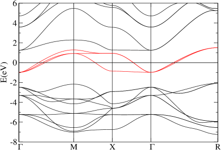
Figure 1: Bandstructure of SrVO₃. Red: $t_{2g}$-bands around the Fermi level.

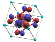
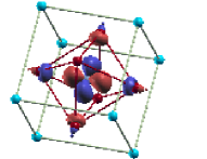
Figure 2: Isosurface plot of the $t_{2g}$-like MLWF $d_{xy}$ for SrVO₃ calculated with spin-orbit coupling. Left: Spin-up component (real part), isosurface=$\pm$0.05. Right: Spin-down component (imaginary part), isosurface=$\pm$0.001. The color of the isosurface refers to the sign: Positive for dark red and negative for dark blue. Red balls: O sites, cyan balls: Sr sites, V site at the center. The WFs were plotted using the program XCrySDen Kokalj (2003).

Table 2: Hopping Integrals for SrVO₃. Energies are in meV.

$xyz$	001	010	011	101	110	111	002	020
$d_{xz},d_{xz}$	$-$262.0	$-$27.0	5.8	$-$84.0	5.8	$-$5.7	7.6	0.2
$d_{xz},d_{yz}$	0.0	0.0	0.0	0.0	9.2	3.6	0.0	0.0

III.2 BaTiO₃

As a simple application of the Wannier-function scheme we present the calculation of the ferroelectric polarization of the ferroelectric perovskite BaTiO₃. The evaluation of the polarization from a DFT calculation of an infinite crystal can be achieved by means of the Berry-phase technique. After the construction of MLWFs for the occupied valence bands this leads to the following expression for the polarization King-Smith and Vanderbilt (1993); Vanderbilt and King-Smith (1993); Marzari and Vanderbilt (1998); Resta (1994); Wu et al. (2006)

$${\bf{P}}=\sum_{i}q_{i}{\bf{X}}_{i}+\sum_{n}e\langle{\bf{x}}\rangle_{n},$$ (41)

where $q_{i}$ and ${\bf{X}}_{i}$ denote charge and position of the ion cores and $\langle{\bf{x}}\rangle_{n}$ are the centers of the occupied Wannier orbitals.

We applied this formalism to strained BaTiO₃ which is assumed to have been grown epitaxially on top of SrTiO₃ assuming the in-plane lattice constant ($a=7.46$ a.u.) of SrTiO₃. We did not consider any finite thickness or interface effects but simply assumed that this epitaxial relation will hold for reasonably thin films. The lattice constant perpendicular ($c$) as well as the positions of all atoms in the unit-cell where then relaxed by a series of force and total energy calculations. For Ba, Ti and O, muffin-tin radii of 2.2 a.u., 2.0 a.u. and 1.3 a.u. were used, respectively. The plane wave cut-off was chosen to be 4.8 a.u.^-1. Using the exchange correlation potential of Perdew and Wang Perdew and Wang (1992) we obtained a $c/a$ ratio of 1.07, in reasonable agreement with experimental data. Petraru et al. (2007) The resulting atomic positions are given in Table 3 and the crystal structure of BaTiO₃ is illustrated in Figures 3 and 4. Compared to the cubic perovskite structure, the oxygen atoms are moved out of the face centers and the cube is elongated in $z$-direction. $z$-reflection symmetry is lost. $\Delta z$ in Table 3 specifies the displacement of the oxygen and titanium atoms from the symmetric positions in the face centers and the center of the cuboid, respectively.

We calculated MLWFs separately for the 9 oxygen $p$-bands, the 3 barium $p$-bands, the 3 oxygen $s$-bands, the one barium $s$-band, and the 3 titanium $p$-bands (the remaining electrons were treated as core electrons) using a uniform $k$-point mesh of 16$\times$16$\times$16 $k$-points. As final spread, Eq. (4), 48.03 a.u.² were obtained for the 9 oxygen $p$ MLWFs while the spread of the first-guess WFs was 48.08 a.u.², demonstrating that first-guess WFs and MLWFs are nearly identical for BaTiO₃. Figures 3 and 4 show the isosurfaces of the resulting MLWFs. The MLWFs clearly reflect the broken $z$-reflection symmetry. Table 4 lists the coordinates of the centers of the MLWFs along with their deviations $\Delta z$ from the ion sites. As evident from there, the oxygen-MLWFs for the site close to the $xy$-plane exhibit the largest response to the broken $z$-reflection symmetry. Applying Eq. (41) we find a polarization of 48.9 $\mu$C/cm² in excellent agreement with experimental data Petraru et al. (2007) of 43 $\mu$C/cm² for the case of thin BaTiO₃ layers grown on SrTiO₃. The displacements of the centers of the MLWFs with respect to the centers of the atoms contribute 36$\%$ to the polarization.

In order to assess convergence of the results with respect to the number of $k$-points a comparative calculation was performed using an 8$\times$8$\times$8 $k$-point mesh. This calculation yielded a final spread of 47.19 a.u.² for the MLWFs of the 9 oxygen $p$ bands and a total polarization of 48.6 $\mu$C/cm². We assume these small differences to be finite difference errors introduced by using formulae Eqns. (5, 6).

Table 3: Positions of the Ba, Ti and O ions in the constrained ferroelectric perovskite BaTiO₃ (atomic units). For the O ions, $\Delta z$ is the displacement from the face centers. For the Ti ion, $\Delta z$ specifies the displacement from the center of the cuboid.

	$x$	$y$	$z$	$\Delta z$
Ba	0.000	0.000	0.000	0.000
Ti	3.730	3.730	3.901	$-$0.092
O	3.730	3.730	0.449	0.449
O	3.730	0.000	4.284	0.292
O	0.000	3.730	4.284	0.292

Table 4: BaTiO₃: Coordinates, displacements and spreads of the MLWFs (atomic units).

	$x$	$y$	$z$	$\Delta z$	$\langle{\bf{x}}^{2}\rangle$
O ($pz$)	3.730	3.730	0.629	0.181	4.75
O ($px$)	3.730	3.730	0.686	0.238	5.69
O ($py$)	3.730	3.730	0.686	0.238	5.69
O ($pz$)	3.730	0.000	4.296	0.012	5.69
O ($px$)	3.730	0.000	4.300	0.016	5.53
O ($py$)	3.730	0.000	4.255	$-$0.029	4.73
O ($pz$)	0.000	3.730	4.296	0.012	5.69
O ($px$)	0.000	3.730	4.255	$-$0.029	4.73
O ($py$)	0.000	3.730	4.300	0.016	5.53
Ba ($pz$)	0.000	0.000	$-$0.047	$-$0.047	6.03
Ba ($px$)	0.000	0.000	$-$0.011	$-$0.011	6.15
Ba ($py$)	0.000	0.000	$-$0.011	$-$0.011	6.15
O ($s$)	3.730	3.730	0.542	0.095	2.77
O ($s$)	3.730	0.000	4.305	0.021	2.64
O ($s$)	0.000	3.730	4.305	0.021	2.64
Ba ($s$)	0.000	0.000	0.000	0.000	3.20
Ti ($pz$)	3.730	3.730	3.863	$-$0.038	1.48
Ti ($px$)	3.730	3.730	3.905	0.003	1.47
Ti ($py$)	3.730	3.730	3.905	0.003	1.47

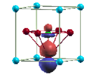
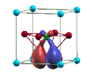
Figure 3: MLWFs $O(p_{z})$ and $O(p_{y})$ for the oxygen site close to $xy$-plane in BaTiO₃. Isosurface=$\pm$0.05. Red balls in the face centers: O sites, cyan balls at the corners: Ba sites, green ball at the center: Ti site. The O site above the upper face of the cuboid is not depicted.

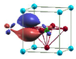
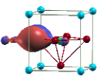
Figure 4: MLWFs $O(p_{z})$, $O(p_{x})$, and $O(p_{y})$ for the oxygen site close to $xz$-plane in BaTiO₃. Isosurface=$\pm$0.05. Red balls in the face centers: O sites, cyan balls at the corners: Ba sites, green ball at the center: Ti site.

III.3 Graphene

Graphene is a covalently bonded system. Consequently, one expects that the MLWFs are bond centered. This is a particularly stringent test for our implementation as the LAPW basis functions in which the BFs are expanded (see Eq. 15) are centered around the atoms. Actually, the four valence bands do not constitute an isolated group of bands as they touch an unoccupied band at the $\overline{K}$-point. Avoiding the $\overline{K}$-point when choosing the uniform $k_{\scriptscriptstyle\|}$-mesh, disentangling is not necessary, however. A single layer of graphene was calculated within the FLEUR film mode. The muffin-tin radii and the plane wave cut-off were chosen to be 1.28 a.u. and 4.6 a.u.^-1, respectively. The C-C bond length was assumed to be 2.72 a.u.. We used the exchage-correlation potential of Perdew, Burke, and Ernzerhof. Perdew et al. (1996) MLWFs and first-guess WFs were constructed for the four valence bands using an 8$\times$8 $k_{\scriptscriptstyle\|}$-mesh in the two-dimensional Brillouin zone. For the construction of the first-guess WFs, two calculations were performed: In one calculation the localized functions $|g_{n}\rangle$ corresponding to the $sp^{2}$-bonds were chosen to be restricted to the muffin-tin sphere of only one atom (FWF1), while they were restricted in the second calculation (FWF2) to the muffin-tins of the two atoms participating in the covalent bonding. The FWF2s were nearly identical with the MLWFs, having the same centers and negligibly different spreads, in particular. The FWF1s are not centered in the middle of the C-C-bond, the FWF2s are, however, centered. Irrespective of the starting point (i.e. either FWF1 or FWF2) we arrive at the same MLWFs, which are bond centered.

Figure 5 shows the contour plot of one of the three $sp^{2}$-bonds for the first-guess FWF1 and for the MLWF. Figure 6 shows the $\pi$-orbital. Centers and spreads are given in Table 5. The initial spread of 17.08 a.u.² characterizing the first-guess FWF1 is reduced by the minimization procedure to a final total spread of 16.23 a.u.².

The hopping matrix elements $H_{m,m^{\prime}}({\bf{R}}_{1}-{\bf{R}}_{2})$, Eq. (29), are listed in Table 6. There is no coupling between the $\pi$ WFs and the $sp^{2}$ WFs.

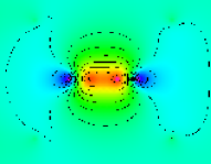
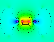
Figure 5: Contour plot of the FWF1 (left) and MLWF (right) of an $sp^{2}$-bond of graphene.

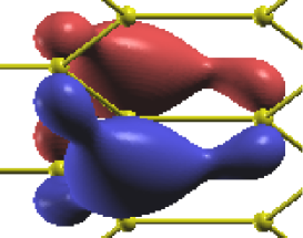
Figure 6: Isosurface plot of the $\pi$-orbital of graphene. Isosurface=$\pm$0.1

Table 5: Centers and spreads of the first-guess (first row) and maximally localized (second row) WFs (atomic units).

	$x$	$y$	$z$	$\langle{\bf{x}}^{2}\rangle$
FWF1 ($sp^{2}$)	2.038	1.169	0.000	2.184
FWF1 ($sp^{2}$)	2.038	$-$1.169	0.000	2.184
FWF1 ($sp^{2}$)	4.064	0.000	0.000	2.184
FWF1 ($\pi$)	2.714	0.000	0.000	10.526
MLWF ($sp^{2}$)	2.035	1.175	0.000	2.052
MLWF ($sp^{2}$)	2.035	$-$1.175	0.000	2.052
MLWF ($sp^{2}$)	4.070	0.000	0.000	2.052
MLWF ($\pi$)	2.714	0.000	0.000	10.075

Table 6: Hopping matrix elements of graphene. Energies are in meV. 00, 10, 11 and 20 denote the translations of the obitals in units of the primitive translations.

	00	10	11	20
$sp^{2}(1),sp^{2}(1)$	-15038	560.7	6.6	51.3
$sp^{2}(1),sp^{2}(2)$	-2139	78.0	-21.5	7.4
$sp^{2}(1),sp^{2}(3)$	-2139	-144.1	2.5	-19.9
$sp^{2}(2),sp^{2}(1)$	-2139	-529.8	-21.5	-21.5
$sp^{2}(2),sp^{2}(2)$	-15038	-109.7	6.6	-6.7
$sp^{2}(2),sp^{2}(3)$	-2139	78.0	2.5	7.4
$sp^{2}(3),sp^{2}(1)$	-2139	-2139.1	78.0	-144.1
$sp^{2}(3),sp^{2}(2)$	-2139	-529.8	78.0	-21.5
$sp^{2}(3),sp^{2}(3)$	-15038	560.7	-16.4	51.3
$\pi,\pi$	-8329	-728.0	162.9	51.6

III.4 Platinum

We close the results section with the discussion of the MLWFs for a Platinum chain. Our calculations were performed with the one-dimensional version Mokrousov et al. (2005) of the FLEUR program and with spin-orbit coupling Delin and Tosatti (2003); Velev et al. (2005); Delin et al. (2004); Mokrousov et al. (2006). The extensions necessary to treat the spin-orbit case have been described in section II.7. The muffin-tin radii and the plane wave cut-off were chosen to be 2.22 a.u. and 3.7 a.u.^-1, respectively. The RPBE Zhang and Yang (1998) exchange-correlation potential was used. The relaxed Pt-Pt distance is given by 4.48 a.u.. We calculated 12 MLWFs corresponding to the $s$- and $d$-states of Platinum using 8 $k$-points. The localized trial orbitals were chosen to be eigenstates of the $z$-projection of the spin operator. Both the direction of the chain and the spin-quantization axis are given by the $z$-direction. We chose the angular parts of the trial-orbitals for the $d$-bands to be $d_{3x^{2}-r^{2}}$, $d_{3y^{2}-r^{2}}$, (i.e. $d_{3z^{2}-r^{2}}$ rotated to be coaxial with the $x$- and $y$-directions, respectively), $d_{xy}$, $d_{xz}$ and $d_{yz}$. The localized trial orbital corresponding to the sp-like WF was constructed as a linear combination of two localized s-orbitals on neighboring atoms. The MLWFs are spinor-valued and complex. 6 out of the 12 MLWFs are characterized by a dominance of the spin-up component while the spin-down component dominates the other 6 MLWFs. The two groups of spin-up and spin-down dominated WFs are symmetric by interchange of spins. Hence we will consider only the 6 spin-up dominated WFs in the following, unless explicitly stated. The angular dependencies of the real parts of the dominating spin-up components are approximately given by $d_{xz}$ and $d_{yz}$, $d_{3x^{2}-r^{2}}$ and $d_{3y^{2}-r^{2}}$, $d_{xy}$, and $sp$. The MLWFs $d_{xz}$, $d_{yz}$ and $d_{3x^{2}-r^{2}}$, $d_{3y^{2}-r^{2}}$ are symmetry equivalent, respectively. The $sp$-like WF is positioned bond-centred between two neighboring Pt-atoms. The angular functions that approximately describe the imaginary part of the spin-up component as well as the real and imaginary parts of the spin-down components agree very well qualitatively with the results of our simple model of section II.7 given in Table 1. We found qualitative deviations only for the $d_{3y^{2}-r^{2}}$-orbital (and the symmetry-equivalent $d_{3x^{2}-r^{2}}$-orbital) shown in Figure 7: While Table 1 predicts the real part of the spin-down component belonging to the $d_{3y^{2}-r^{2}}$-orbital to vanish, it turns out to be non-vanishing and $d_{xz}$-like. This may be attributed to the fact that the actual $d_{3y^{2}-r^{2}}$-like orbital is not rotationally invariant around the $y$-axis, but rather squeezed in $x$-direction. The $d_{xy}$-like WF is shown in Figure 8. As there is no spin-orbit coupling for $s$-states the spin-down component of the $sp$-like WF, which is shown in Figure 9, is $p$-like.

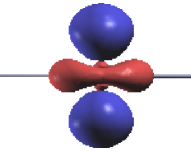
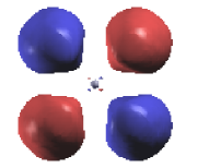
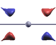
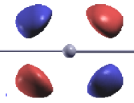
Figure 7: $d_{3y^{2}-r^{2}}$-like orbital of a one-dimensional Pt-chain. Top row: Left: Real part of spin-up component ($d_{3y^{2}-r^{2}}$, Isosurface=$\pm$0.1), Right: imaginary part of spin-up component ($d_{xy}$, Isosurface=$\pm$0.001). Bottom row: Left: Real part of spin-down component ($d_{xz}$, Isosurface=$\pm$0.00073), Right: imaginary part of spin-down component ($d_{yz}$, Isosurface=$\pm$0.0025).

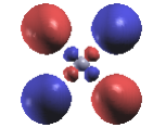
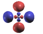
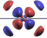
Figure 8: $d_{xy}$-like orbital of a one-dimensional Pt-chain. From left to right: Real part of spin-up component ($d_{xy}$, Isosurface=$\pm$0.2), imaginary part of spin-up component ($d_{x^{2}-y^{2}}$, Isosurface=$\pm$0.005), real part of spin-down component ($d_{yz}$, Isosurface=$\pm$0.001).

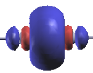
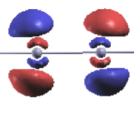
Figure 9: $sp$-like orbital of a one-dimensional Pt-chain. Left: real part of spin-up component ($sp$, Isosurface=$\pm$0.04), Right: real part of spin-down component ($p_{x}$, Isosurface=$\pm$0.004).

Table 7 lists the spreads. The maximal localization procedure reduces the initial total spread of 195.72 a.u.² to a final total spread of 37.56 a.u.².

In Table 8 we list the spin-resolved nearest neighbor hopping matrix elements for the spin-up dominated MLWFs between identical orbitals calculated according to Eq. (33). As the $(\downarrow,\downarrow)$ components scale quadratically with the admixture of spin-down to the spin-up dominated WFs, they are small. Likewise the $(\uparrow,\downarrow)$ components are found to be small: The angular distributions of the spin-down components of the WFs differ from those of the spin-up components, the admixture of spin-down is small, and the spin-orbit coupling, which couples the two spin-channels, is important only close to the nuclear cores and hence the coupling between functions well-localized on different atoms is small. For the on-site hopping matrix elements, however, the $(\uparrow,\downarrow)$- or $(\downarrow,\uparrow)$-components can dominate, because the two WFs are centered on the same atoms in this case, and their overlap close to the nuclear cores can be large. In Table 9 we list a selection of spin-resolved on-site hopping matrix elements that are dominated by hopping from spin-up into spin-down, which is mediated by spin-orbit coupling. $d^{\uparrow}_{xz}$ is a spin-up dominated $d_{xz}$-like WF. According to Table 1 the spin-orbit interaction provides a coupling to $d_{x^{2}-y^{2}}|\downarrow\rangle$, which overlaps with $d^{\downarrow}_{3x^{2}-r^{2}}$. Analogously, there is a transition from $d^{\uparrow}_{3y^{2}-r^{2}}$ to $d_{yz}|\downarrow\rangle$, which overlaps with $d^{\downarrow}_{yz}$. The other two examples in Table 9 are easily interpreted analogously on the basis of Table 1. The $(\downarrow,\uparrow)$-contributions in Table 9 are negligibly small, because the $|\downarrow\rangle$- and $|\uparrow\rangle$-components of the spin-up and spin-down dominated WFs are small, respectively. Table 10 is analogous to Table 8, but now for the nearest neighbor hoppings. The comparison of the two Tables shows that the $(\uparrow,\downarrow)$-contributions decay fastest, which is consistent with the facts that the spin-orbit coupling is strongest close to the nucleii, and that the WFs are well localized.

Table 7: Platinum chain: Spreads of the MLWFs (atomic units).

	$d_{xz}$	$d_{3x^{2}-r^{2}}$	$d_{xy}$	$sp$
$\langle{\bf{x}}^{2}\rangle$	3.336	2.416	2.326	4.952

Table 8: Platinum chain: Spin-resolved nearest neighbor hopping matrix elements for the spin-up dominated MLWFs between identical orbitals (meV).

	$d_{xz}$, $d_{xz}$	$d_{3x^{2}-r^{2}}$, $d_{3x^{2}-r^{2}}$	$d_{xy}$, $d_{xy}$	$s$, $s$
$\uparrow,\uparrow$	1170.9	-548.8	-269.7	-2481.7
$\uparrow,\downarrow$	-0.1	0.4	-0.1	29.3
$\downarrow,\downarrow$	1.0	-0.6	-0.7	-21.3

Table 9: Platinum chain: Spin-resolved on-site hopping matrix elements between spin-up and spin-down dominated MLWFs (meV).

	$d^{\uparrow}_{xz}$, $d^{\downarrow}_{3x^{2}-r^{2}}$	$d^{\uparrow}_{3y^{2}-r^{2}}$,$d^{\downarrow}_{yz}$	$d^{\uparrow}_{xz}$, $d^{\downarrow}_{xy}$	$d^{\uparrow}_{xy}$,$d^{\downarrow}_{xz}$
$\uparrow,\uparrow$	-142	134	10	-6
$\uparrow,\downarrow$	460	460	268	268
$\downarrow,\uparrow$	0	0	0	0
$\downarrow,\downarrow$	134	-142	-6	10

Table 10: Platinum chain: Spin-resolved nearest neighbor hopping matrix elements between spin-up and spin-down dominated MLWFs (meV).

	$d^{\uparrow}_{xz}$, $d^{\downarrow}_{3x^{2}-r^{2}}$	$d^{\uparrow}_{3y^{2}-r^{2}}$,$d^{\downarrow}_{yz}$	$d^{\uparrow}_{xz}$, $d^{\downarrow}_{xy}$	$d^{\uparrow}_{xy}$,$d^{\downarrow}_{xz}$
$\uparrow,\uparrow$	33	0.8	5.6	-9.0
$\uparrow,\downarrow$	9.8	9.8	7.5	7.5
$\downarrow,\uparrow$	0	0	0	0
$\downarrow,\downarrow$	0.8	33	-9.0	5.6

IV Conclusions

We have described the implementation of Wannier functions within the FLAPW program FLEUR for bulk, film and wire geometry. Two kinds of WFs with optimized localization properties – the first-guess and the maximally localized Wannier functions – have been described and calculated for four concrete systems, SrVO₃, BaTiO₃, graphene and platinum. Our results are in very good agreement to previous ones, where available, including the ferroelectric polarization of BaTiO₃. We found the first-guess WFs and the MLWFs to be similar for the first three systems, and rather different for Pt. While in cases where the first-guess WFs and the MLWFs do not differ substantially there is the option to use the first-guess WFs in practice for certain applications, which is computationally less demanding, the extended scheme needed for the construction of the MLWFs still proves valuable if quantities such as the electric polarization are supposed to be extracted.

Appendix A Vacuum contributions to the $M_{mn}^{({\bf{k}},{\bf{b}})}$ matrix in case of film calculations

In case of the film implementation of the FLAPW method, an additional semi-infinite vacuum region is present, which results in an additional contribution to the wave function overlaps $M_{mn}^{({\bf{k}},{\bf{b}})}|_{\text{VAC}}$. In this appendix we give explicit expressions for the vacuum contributions to the $M_{mn}^{({\bf{k}},{\bf{b}})}$ matrix elements.

In the film geometry, the interstitial region stretches in z-direction from $-D/2$ to $D/2$, which is chosen to be the direction orthogonal to the film. Thus, one of the two vacua extends from $-\infty$ to $-D/2$ while the second vacuum extends from $D/2$ to $+\infty$. The two vacua are treated analogously and we will restrict the discussion to the vacuum between $D/2$ and $+\infty$. According to the topology of the vacuum region, the Bloch wave functions in the vacuum are represented in the following way:

$$\psi_{{\bf{k_{\|}}}m}({\bf{x}})|_{\text{VAC}}=\sum_{{\bf{G_{\|}}}}\Psi^{m}_{{\bf{G_{\|}}}}({\bf{k_{\|}}},z)e^{i({\bf{G_{\|}}}+{\bf{k_{\|}}})\cdot{\bf{x}}_{\|}},$$ (42)

with

$$\Psi^{m}_{{\bf{G_{\|}}}}({\bf{k}}_{\|},z)=A^{m}_{{\bf{G_{\|}}}}({\bf{k}}_{\|})u_{{\bf{G_{\|}}}}^{{\bf{k}}_{\|}}(z)+B^{m}_{{\bf{G_{\|}}}}({\bf{k}}_{\|})\dot{u}_{{\bf{G_{\|}}}}^{{\bf{k}}_{\|}}(z),$$ (43)

where ${\bf{G}}=({\bf{G_{\|}}},G_{z})$ and ${\bf{x}}=({\bf{x}}_{\|},z)$ have been used, with ${\bf{G_{\|}}}$ and ${\bf{x_{\|}}}$ the in-plane components. The $k$-point ${\bf{k}}_{\|}$ belongs to the two-dimensional BZ. $u_{{\bf{G_{\|}}}}^{{\bf{k}}}(z)$ and $\dot{u}_{{\bf{G_{\|}}}}^{{\bf{k}}}(z)$ are the solution of the one-dimensional Schrödinger equation in the vacuum and its energy derivative, respectively. Substituting Eq. 42 into Eq. 13 yields:

$$M_{mn}^{({\bf{k}}_{\|},{\bf{b}})}$$ (44)

$$=\sum_{{\bf{G_{\|}}},{\bf{G^{\prime}_{\|}}}}\int_{\text{VAC}} e^{i{\bm{\mathcal{G}}}\cdot{\bf{x}}}(\Psi^{m}_{{\bf{G_{\|}}}}({\bf{k}}_{\|},z))^{*}\Psi^{n}_{{\bf{G^{\prime}_{\|}}}}([{\bf{k}}_{\|}+{\bf{b}}],z)\,d^{3}x$$

with ${\bm{\mathcal{G}}}={\bf{G^{\prime}_{\|}}}-{\bf{G_{\|}}}-{\bf{G}}({\bf{k}}_{\|}+{\bf{b}})$. While vectors ${\bf{k}}_{\|}$ and $[{\bf{k}}_{\|}+{\bf{b}}]$ always lie in the two-dimensional Brillouin zone, the ${\bf{b}}$ and ${\bf{G}}({\bf{k}}_{\|}+{\bf{b}})$ vectors have a $z$-component in general, which leads to the following expression for the $M_{mn}^{({\bf{k}}_{\|},{\bf{b}})}$ matrix elements:

$$M_{mn}^{({\bf{k}}_{\|},{\bf{b}})}=\sum_{{\bf{G_{\|}}},{\bf{G^{\prime}_{\|}}}}S_{\|}\delta_{{\bm{\mathcal{G}}}_{\|}}$$ (45)

$$\times\int^{\infty}_{D/2} e^{-i\,G_{z}({\bf{k}}_{\|}+{\bf{b}})\,z}(\Psi^{m}_{{\bf{G_{\|}}}}({\bf{k}}_{\|},z))^{*}\Psi^{n}_{{\bf{G^{\prime}_{\|}}}}([{\bf{k}}_{\|}+{\bf{b}}],z)\,dz,$$

with $S_{\|}$ being the in-plane unit-cell area, and the last integral is a linear combination of one-dimensional integrals of the form

$$\int^{\infty}_{D/2}e^{-i\,G_{z}({\bf{k}}_{\|}+{\bf{b}})\,z}\,u_{{\bf{G_{\|}}}}^{{\bf{k}}_{\|}}(z)\,u_{{\bf{G^{\prime}_{\|}}}}^{[{\bf{k}}_{\|}+{\bf{b}}]}(z)\,dz,$$ (46)

$$\int^{\infty}_{D/2}e^{-i\,G_{z}({\bf{k}}_{\|}+{\bf{b}})\,z}\,u_{{\bf{G_{\|}}}}^{{\bf{k}}_{\|}}(z)\,\dot{u}_{{\bf{G^{\prime}_{\|}}}}^{[{\bf{k}}_{\|}+{\bf{b}}]}(z)\,dz,$$

which are easily computed numerically for every pair of $({\bf{G_{\|}}},{\bf{G^{\prime}_{\|}}})$.

Appendix B Vacuum contributions to the $M_{mn}^{({\bf{k}},{\bf{b}})}$ matrix in case of one dimensional calculations

In the case of the one-dimensional setup the vacuum region surrounds a cylinder with the symmetry axis along the $z$-direction and radius $R_{\text{vac}}$. The wave function in the vacuum is represented in the following form (in the 1D case the Bloch vector is ${\bf{k}}=(0,0,k_{z})$):

$$\begin{array}[]{cc}\displaystyle\psi_{k_{z}m}({\bf{x}})=\sum_{G_{z},p}(A_{p,G_{z}}^{m,k_{z}}u_{p}^{G_{z}}(k_{z},r)+B_{p,G_{z}}^{m,k_{z}}\dot{u}_{p}^{G_{z}}(k_{z},r))\times\\[8.5359pt] \displaystyle\times e^{ip\varphi}e^{i(G_{z}+k_{z})z},\end{array}$$ (47)

where ${\bf{x}}=(z,r,\varphi)$ in cylindrical coordinates, $G_{z}$ is the $z$-component of the reciprocal vector ${\bf{G}}$, and $p$ is an integer number labeling a cylindrical angular harmonic. The exponentially decaying functions $u$ and $\dot{u}$ are the solutions of the radial equation for the vacuum and its energy derivative, respectively. Taking into account the expansion of a plane wave in cylindrical coordinates

$$e^{i{\bf{G}}{\bf{x}}}=e^{iG_{z}z}\sum_{p}\,i^{p}e^{ip(\varphi-\varphi_{{\bf{G}}})}J_{p}(G_{r}r),$$ (48)

with $\varphi_{{\bf{G}}}$ and $G_{r}$ being cylindrical angular and radial coordinates, respectively, of the vector ${\bf{G}}=(G_{z},G_{r},\varphi_{{\bf{G}}})$ in reciprocal space, and $J_{p}$ standing for the cylindrical Bessel function of order $p$, the 1D-vacuum contribution to the $M_{mn}^{(k_{z},{\bf{b}})}$ matrix reads:

$$\begin{array}[]{cc}\displaystyle M_{mn}^{(k_{z},{\bf{b}})}|_{\text{VAC}}=\int_{\text{VAC}}e^{-i{\bf{b}}\cdot{\bf{x}}}(\psi_{k_{z}m}({\bf{x}}))^{*}\psi_{[k_{z}+{\bf{b}}],n}({\bf{x}})\,d^{3}x\\[14.22636pt] =\displaystyle\sum_{G_{z},G^{\prime}_{z}}\sum_{p,p^{\prime}}\int_{\text{VAC}}e^{i(G^{{}^{\prime}}_{z}-G_{z}-G_{z}(k_{z}+{\bf{b}}))z}\times\\[19.91684pt] \displaystyle\times\,e^{-i{\bf{G}}_{\|}(k_{z}+{\bf{b}}){\bf{x}}_{\|}}\,e^{i(p^{\prime}-p)\varphi}\,\Psi_{p,p^{\prime},G^{\prime}_{z}}^{m,n,G_{z}}(k_{z},[k_{z}+{\bf{b}}],r)\,d^{3}x,\end{array}$$ (49)

where in analogy to the case of the film geometry, vectors ${\bf{b}}$ and ${\bf{G}}(k_{z}+{\bf{b}})$ may have a non-zero component in the plane normal to the $z$-axis, and the function $\Psi$ is constructed from the products of the $u$- and $\dot{u}$-functions with corresponding $A$- and $B$-coefficients at $k$-points $k_{z}$ and $[k_{z}+{\bf{b}}]$. Introducing the vector $\mathcal{G}=G^{{}^{\prime}}_{z}-G_{z}-G_{z}(k_{z}+{\bf{b}})$ the expression for the $M_{mn}^{(k_{z},{\bf{b}})}$ can be reduced to

$$\begin{array}[]{cc}\displaystyle M_{mn}^{(k_{z},{\bf{b}})}|_{\text{VAC}}=\sum_{G_{z},G^{{}^{\prime}}_{z}}\sum_{p,p^{\prime}}\mathcal{S}\cdot\delta_{\mathcal{G}}\cdot i^{p-p^{\prime}}e^{-i(p-p^{\prime})\varphi_{{\bf{G}}(k_{z}+{\bf{b}})}}\times\\[14.22636pt] \displaystyle\times\int_{R_{\text{vac}}}^{\infty}rJ_{p^{\prime}-p}(G_{r}(k_{z}+{\bf{b}})r)\Psi_{p,p^{\prime},G^{\prime}_{z}}^{m,n,G_{z}}(k_{z},[k_{z}+{\bf{b}}],r)\,dr,\end{array}$$ (50)

with $\mathcal{S}=2\pi T$, and $T$ standing for the lattice constant of the system under consideration along the $z$-axis.

Appendix C Local orbital contributions to the $M_{mn}^{({\bf{k}},{\bf{b}})}$ matrix

In order to increase the variational freedom of the FLAPW-basis or to describe semicore levels adequately, it may be supplemented by local orbitals. Singh (1991) In this case the expressions for the BFs in the spheres are modified:

$$\begin{array}[]{cc}\displaystyle\psi_{{\bf{k}}m}({\bf{x}})|_{\text{MT}^{\mu}}=\sum_{L}(A^{\mu}_{L,m}({\bf{k}})u_{l}^{\mu}(r)+B^{\mu}_{L,m}({\bf{k}})\dot{u}_{l}^{\mu}(r))Y_{L}(\hat{{\bf{r}}})\\ \displaystyle+\sum_{Lo}C^{\mu}_{Lo,m}({\bf{k}})u_{lo}^{\mu}(r)Y_{Lo}(\hat{{\bf{r}}}),\end{array}$$ (51)

where $Lo=(lo,mo)$ stands for the corresponding values of the angular quantum numbers $(l,m)$ assigned to each local orbital. Due to the local orbitals, additional terms arise in the expression Eq. 17 for the $M_{mn}^{({\bf{k}},{\bf{b}})}|_{\text{MT}^{\mu}}$ matrix:

$$\begin{array}[]{cc}M_{mn}^{({\bf{k}},{\bf{b}})}|^{Lo}_{\text{MT}^{\mu}}=4\pi e^{-i{\bf{b}}\cdot{\bm{\tau}}_{\mu}}\times\\[5.69046pt] \displaystyle\times(\sum_{L,Lo^{\prime}}(A^{\mu}_{L,m}({\bf{k}}))^{*}C^{\mu}_{Lo^{\prime},m}({\bf{[k+b]}})\,t_{11}^{\mu}({\bf{b}},L,Lo^{\prime})+\\ \displaystyle+\sum_{L,Lo^{\prime}}(B^{\mu}_{L,m}({\bf{k}}))^{*}C^{\mu}_{Lo^{\prime},m}({\bf{[k+b]}})\,t_{21}^{\mu}({\bf{b}},L,Lo^{\prime})+\\ \displaystyle+\sum_{Lo,L^{\prime}}(C^{\mu}_{Lo,m}({\bf{k}}))^{*}A^{\mu}_{L^{\prime},m}({\bf{[k+b]}})\,t_{11}^{\mu}({\bf{b}},Lo,L^{\prime})+\\ \displaystyle+\sum_{Lo,L^{\prime}}(C^{\mu}_{Lo,m}({\bf{k}}))^{*}B^{\mu}_{L^{\prime},m}({\bf{[k+b]}})\,t_{12}^{\mu}({\bf{b}},Lo,L^{\prime})+\\ \displaystyle+\sum_{Lo,Lo^{\prime}}(C^{\mu}_{{Lo},m}({\bf{k}}))^{*}C^{\mu}_{Lo^{\prime},m}({\bf{[k+b]}})\,t_{11}^{\mu}({\bf{b}},Lo,Lo^{\prime})),\end{array}$$ (52)

where the corresponding radial function for the local orbital is taken in the $t_{ij}^{\mu}$-integrals, whenever a radial function $u$ has an index $lo$.

References

- (1) In the case of spin-orbit coupling, for example, the requirement of real-valuedness of the Wannier function cannot be fulfilled in general.
- Wannier (1937) G. H. Wannier, Phys. Rev. 52, 191 (1937).
- Andersen and Saha-Dasgupta (2000) O. K. Andersen and T. Saha-Dasgupta, Phys. Rev. B 62, 16219 (2000).
- Pavarini et al. (2005) E. Pavarini, A. Yamasaki, J. Nuss, and O. K. Andersen, New J. Phys. 7, 188 (2005).
- Zurek et al. (2005) E. Zurek, O. Jepsen, and O. K. Andersen, ChemPhysChem 6, 1934 (2005).
- Marzari and Vanderbilt (1997) N. Marzari and D. Vanderbilt, Phys. Rev. B 56, 12847 (1997).
- Souza et al. (2001) I. Souza, N. Marzari, and D. Vanderbilt, Phys. Rev. B 65, 035109 (2001).
- King-Smith and Vanderbilt (1993) R. D. King-Smith and D. Vanderbilt, Phys. Rev. B 47, 1651 (1993).
- Vanderbilt and King-Smith (1993) D. Vanderbilt and R. D. King-Smith, Phys. Rev. B 48, 4442 (1993).
- Marzari and Vanderbilt (1998) N. Marzari and D. Vanderbilt, in First-Principles Calculations for Ferroelectrics: Fifth Williamsburg Workshop (Springer Verlag, 1998), p. 146.
- Resta (1994) R. Resta, Rev. Mod. Phys. 66, 899 (1994).
- Wu et al. (2006) X. Wu, O. Diéguez, K. M. Rabe, and D. Vanderbilt, Phys. Rev. Lett. 97, 107602 (2006).
- Thonhauser et al. (2005) T. Thonhauser, D. Ceresoli, D. Vanderbilt, and R. Resta, Phys. Rev. Lett. 95, 137205 (2005).
- Ceresoli et al. (2006) D. Ceresoli, T. Thonhauser, D. Vanderbilt, and R. Resta, Phys. Rev. B 74, 024408 (2006).
- Silvestrelli et al. (1998) P. L. Silvestrelli, N. Marzari, D. Vanderbilt, and M. Parrinello, Solid State Communications 107, 7 (1998).
- Thygesen and Jacobsen (2005) K. S. Thygesen and K. W. Jacobsen, Chemical Physics 319, 111 (2005).
- Calzolari et al. (2004) A. Calzolari, N. Marzari, I. Souza, and M. B. Nardelli, Phys. Rev. B 69, 035108 (2004).
- Pavarini et al. (2004) E. Pavarini, S. Biermann, A. Poteryaev, A. I. Lichtenstein, A. Georges, and O. K. Andersen, Phys. Rev. Lett. 92, 176403 (2004).
- Anisimov et al. (2005) V. I. Anisimov, D. E. Kondakov, A. V. Kozhevnikov, I. A. Nekrasov, Z. V. Pchelkina, J. W. Allen, S.-K. Mo, H.-D. Kim, P. Metcalf, S. Suga, et al., Phys. Rev. B 71, 125119 (2005).
- Lechermann et al. (2006) F. Lechermann, A. Georges, A. Poteryaev, S. Biermann, M. Posternak, A. Yamasaki, and O. K. Andersen, Phys. Rev. B 74, 125120 (2006).
- Posternak et al. (2002) M. Posternak, A. Baldereschi, S. Massidda, and N. Marzari, Phys. Rev. B 65, 184422 (2002).
- Cangiani et al. (2004) G. Cangiani, A. Baldereschi, M. Posternak, and H. Krakauer, Phys. Rev. B 69, 121101 (2004).
- Posternak et al. (2006) M. Posternak, A. Baldereschi, E. J. Walter, and H. Krakauer, Phys. Rev. B 74, 125113 (2006).
- (24) See http://www.flapw.de.
- Krakauer et al. (1979) H. Krakauer, M. Posternak, and A. J. Freeman, Phys. Rev. B 19, 1706 (1979).
- Mokrousov et al. (2005) Y. Mokrousov, G. Bihlmayer, and S. Blügel, Phys. Rev. B 72, 045402 (2005).
- Kohn (1959) W. Kohn, Phys. Rev. 115, 809 (1959).
- (28) Wannier90 code, (See: http://www.wannier.org/).
- Ren et al. (2006) X. Ren, I. Leonov, G. Keller, M. Kollar, I. Nekrasov, and D.Vollhardt, Phys. Rev. B 74, 195114 (2006).
- Hamann (1979) D. R. Hamann, Phys. Rev. Lett. 42, 662 (1979).
- Wimmer et al. (1981) E. Wimmer, H. Krakauer, M. Weinert, and A. J. Freeman, Phys. Rev. B 24, 864 (1981).
- Perdew et al. (1996) J. P. Perdew, K. Burke, and M. Ernzerhof, Phys. Rev. Lett. 77, 3865 (1996).
- Kokalj (2003) A. Kokalj, Comp. Mater. Sci. 28, 155 (2003), code available from http:/www.xcrysden.org/.
- Perdew and Wang (1992) J. P. Perdew and Y. Wang, Phys. Rev. B 45, 13244 (1992).
- Petraru et al. (2007) A. Petraru, N. A. Pertsev, H. Kohlstedt, U. Poppe, R. Waser, A. Solbach, and U. Klemradt, J. App. Phys. 101, 114106 (2007).
- Delin and Tosatti (2003) A. Delin and E. Tosatti, Phys. Rev. B 68, 144434 (2003).
- Velev et al. (2005) J. Velev, R. F. Sabirianov, S. S. Jaswal, and E. Y. Tsymbal, Phys. Rev. Lett. 94, 127203 (2005).
- Delin et al. (2004) A. Delin, E. Tosatti, and R. Weht, Phys. Rev. Lett. 92, 057201 (2004).
- Mokrousov et al. (2006) Y. Mokrousov, G. Bihlmayer, S. Heinze, and S. Blügel, Phys. Rev. Lett. 96, 147201 (2006).
- Zhang and Yang (1998) Y. Zhang and W. Yang, Phys. Rev. Lett. 80, 890 (1998).
- Singh (1991) D. Singh, Phys. Rev. B 43, 6388 (1991).