On a quantum model of a laser-interferometer measuring a weak classical force

Abstract

We consider a solvable model of a laser-interferometer measuring a weak classical force. The model takes into account dissipation of the energy by transfer to the environment at zero temperature. The sensitivity (the signal-to-noise ratio) of the device is defined as the corresponding ratio between the mean value and the variance of a certain observable. We analyze the dependence of the sensitivity upon the duration of the measurement and the photon number. For parameters typical for the LIGO project, we discuss numerical estimates.

1 Introduction

In this paper, we consider the measurement of a weak classical force perturbed by quantum effects. The measuring device consists of a suspended mirror considered as a quantum oscillator driven by a classical force, and a recording device which produces the reduction of the sensor state.

The coherent electromagnetic field, considered as a sensor, is enclosed in the cavity between the movable and the fixed mirrors. Any displacement of the oscillator changes the phase of the wave leaving the cavity. The phase is measured by the interferometer, and the output signal provides an information about the classical force. We assume that the interaction between the oscillator and the environment is irreversible: dissipation of the energy is the result of spontaneous transfer of internal mechanical tensions in the suspension of the mirror to acoustic waves. By this reason, we treat the oscillator as an open quantum system and its states as solutions of the master Markov equation [1].

Under sufficiently general assumptions, the evolving state obeys the Lindblad equation [2]

$$\frac{d}{dt}\rho_{t}=\mathcal{L}^{\dagger}(\rho_{t})\,,\qquad\mathcal{L}^{\dagger}(\rho_{t})=\Phi^{\dagger}(\rho_{t})-\Phi(I)\circ\rho_{t}-\frac{i}{\hbar}[\widehat{H},\rho_{t}]\,,$$ (1)

where $\widehat{H}$ is the system Hamiltonian describing the reversible dynamics, $\Phi(\cdot)$ is a certain completely positive map describing dissipative processes, $\Phi^{\dagger}(\cdot)$ is the completely positive map dual to $\Phi(\cdot)$. The duality is established by the trace:

$$\mathrm{Tr}\,\Phi^{\dagger}(\rho)\sigma=\mathrm{Tr}\,\rho\Phi(\sigma).$$

$A\circ B=\frac{1}{2}(AB+BA)$ is the symmetric Jordan product.

The specific form of the map $\mathcal{L}^{\dagger}$ can be deduced from a physical model of a coupling between the system and the environment [3]. For example, the intensity of the dissipative transfer of the energy is proportional to the energy of the state, and the evolution of any state to the ground state (zero temperature) is described by a CCP Lindblad generator:

$${\cal L}_{0}^{\dagger}(\rho_{t})=\lambda\left(b\rho_{t}b^{\dagger}-\frac{1}{2}(\rho_{t}b^{\dagger}b+b^{\dagger}b\rho_{t})\right)\,,$$ (2)

where $\lambda>0$ is the dissipation rate, i.e. the mean number of quantums of energy transferred per unit of time to the environment, $b^{\dagger}\text{ and }b$ are the creation and annihilation operators, $b^{\dagger}b$ is the energy of the oscillator.

If the reservoir has a nonzero temperature, the generator driving the compound system to the equilibrium has the form [4, 5]:

$${\cal L}_{\nu}^{\dagger}(\rho_{t})=\frac{\lambda}{2}(\nu+1)(2b\rho_{t}b^{\dagger}-b^{\dagger}b\rho_{t}-\rho_{t}b^{\dagger}b)+\frac{\lambda}{2}\nu(2b^{\dagger}\rho_{t}b-bb^{\dagger}\rho_{t}-\rho_{t}bb^{\dagger})\,.$$ (3)

The mean energy of the quantum oscillator with eigenfrequency $\Omega$ in the balanced state with such environment is equal to $E_{0}=\hbar\Omega\nu$.

This paper extends our previous work [6]. In the first section, we describe a mathematical model of the oscillator interacting with the laser radiation and a classical force, but unlike [6], we take into account the transfer of the energy to the environment at zero temperature. For the product system consisting of the oscillator and the electromagnetic field, we derive an explicit form of the density matrix.

This solution is applied to calculation of the mean value of the intensity and the variance of varying photon flow at the output of a twin-wave interferometer of a Michelson or Mach-Zehnder type. In comparison with [6], here we use an observable which properly takes into account the two-beam quantum interference.

In the third section, we consider relative fluctuations of the signal. Numerical estimates of the sensitivity are based on realistic data describing the LIGO detector. Physically motivated estimates of the sensitivity of such devices based on spectral representation can be found in [7], [8].

2 Solvable model

Consider the coherent electromagnetic field with frequency $\omega$ between a movable mirror and a fixed one. Let a small classical external force act on the movable mirror. By $a^{\dagger}\text{ and }a$ we denote the creation and annihilation operators of the radiation in the cavity, and $b^{\dagger}\text{ and }b$ stand for the creation and annihilation operators of the quantum oscillator (the movable mirror) with eigenfrequency $\Omega$.

The reversible dynamics of the laser radiation and the oscillator in the Hilbert space $l_{2}\otimes l_{2}$ (the first factor corresponds to the space of radiation states, and the second one corresponds to that of the oscillator) is described by the generator consisting of three summands [9, 10]

$$H_{t}=\hbar\left[\omega a^{\dagger}a\otimes I+I\otimes\Omega b^{\dagger}b+(g\,a^{\dagger}a+f(t))\otimes(b^{\dagger}+b)\right],$$ (4)

where the first two terms are the energy operators of the radiation and the oscillator, and the third one is the energy of the oscillator due to the radiation pressure and an external force, $\hat{x}=\frac{b^{\dagger}+b}{\sqrt{2}}$ is the position operator of the movable mirror. We used the following notation:

$$g=\frac{\omega}{L}\sqrt{\frac{2\hbar}{m\Omega}}$$ (5)

is the constant of coupling between the laser radiation and the oscillator,

$$f(t)=\frac{F(t)}{\sqrt{2m\Omega\hbar}},$$ (6)

$F(t)$ is a classical force, $m$ is the mass of the mirror, $L$ is the distance between the mirrors. In accordance with (1) and (2), the evolution of the system with Hamiltonian (4) and dissipation of the energy to the environment at zero temperature is described by a quantum master equation

$$\frac{d}{dt}\rho_{t}=-\frac{i}{\hbar}[H_{t},\rho_{t}]-\frac{\lambda}{2}(b^{\dagger}b\rho_{t}+\rho_{t}b^{\dagger}b-2b\rho_{t}b^{\dagger}),\quad\rho_{t}\bigl{|}_{t=0}=\rho_{0}.$$ (7)

We look for the solution of this equation in the following form [11]:

$$\rho_{t}=\mathbb{E}\,u_{t}\rho_{0}u_{t}^{*}\,,$$ (8)

where $u_{t}$ is an operator-valued stochastic function satisfying the stochastic Schrödinger equation

$$du_{t}=\left[\left(-\frac{\lambda}{2}b^{\dagger}b-i\Omega\,b^{\dagger}b-i\omega a^{\dagger}a-i\left(g\,a^{\dagger}a+f(t)\right)(b^{\dagger}+b)\right)dt+\sqrt{\lambda}\,b\,dw_{t}\right]u_{t},$$ (9)

with initial condition $u_{0}=I$. $w_{t}$ stands for the standard Wiener process. The representation (8), (9) for the solution of (7) is well known ([3], [4]); it follows from the Ito differentiation rule [12].

Passing to the interaction representation [6], setting $v_{t}\stackrel{{\scriptstyle\text{{def}}}}{{=}}e^{i\omega a^{\dagger}a\,t}e^{(i\Omega+\frac{\lambda}{2})b^{\dagger}b\,t}u_{t}$, we have

$$d\,v_{t}=\left[-i\bigl{(}ga^{\dagger}a+f(t)\bigr{)}(be^{-(i\Omega+\frac{\lambda}{2})t}+b^{\dagger}e^{(i\Omega+\frac{\lambda}{2})t})dt+\sqrt{\lambda}be^{-(i\Omega+\frac{\lambda}{2})t}dw_{t}\right]v_{t}.$$

Then, $\phi_{t}\stackrel{{\scriptstyle\text{{def}}}}{{=}}e^{ib^{\dagger}\beta^{+}_{t}}v_{t}$, so we obtain

$$d\phi_{t}=\left[-i(ga^{\dagger}a+f(t))(b-i\beta^{+}_{t})e^{-(i\Omega+\frac{\lambda}{2})t})dt+\sqrt{\lambda}(b-i\beta^{+}_{t})e^{-(i\Omega+\frac{\lambda}{2})t}dw_{t}\right]\phi_{t}.$$

In the above equation, all summands commute. The notation $\beta^{\pm}_{t}$ is used for the following family of commuting operators:

$$\beta^{\pm}_{t}=\int\limits_{0}^{t}(ga^{\dagger}a+f(\tau))e^{\pm(i\Omega+\frac{\lambda}{2})\tau}d\tau.$$ (10)

Picking out a stochastic part of the solution, we obtain an equation for $\xi_{t}\stackrel{{\scriptstyle def}}{{=}}e^{ib\beta^{-}_{t}}e^{C_{t}}\phi_{t}$:

$$d\xi_{t}=\sqrt{\lambda}(b-i\beta^{+}_{t})e^{-(i\Omega+\frac{\lambda}{2})t}\xi_{t}dw_{t},\quad C_{t}=\int\limits_{0}^{t}(ga^{\dagger}a+f(\tau))e^{-(i\Omega+\frac{\lambda}{2})\tau}\beta^{+}_{\tau}d\tau.$$ (11)

The solution $\xi_{t}$ is a stochastic process which has the form of the operator-valued Girsanov functional [13]:

$$\xi_{t}=e^{\sqrt{\lambda}\int_{0}^{t}(b-i\beta^{+}_{\tau})e^{-(i\Omega+\frac{\lambda}{2})\tau}dw_{\tau}}e^{-\frac{\lambda}{2}\int_{0}^{t}(b-i\beta^{+}_{\tau})^{2}e^{-2(i\Omega+\frac{\lambda}{2})\tau}d\tau}.$$

Finally, the solution of equation (9) reads as the following normally ordered composition of exponents:

$$u_{t} =e^{-i\omega a^{\dagger}a\,t}e^{-(i\Omega+\frac{\lambda}{2})b^{\dagger}b\,t}e^{-ib^{\dagger}\beta^{+}_{t}}e^{-ib\beta^{-}_{t}}e^{-C_{t}}$$

$$\times e^{\sqrt{\lambda}\int_{0}^{t}(b-i\beta^{+}_{\tau})e^{-(i\Omega+\frac{\lambda}{2})\tau}dw_{\tau}}e^{-\frac{\lambda}{2}\int_{0}^{t}(b-i\beta^{+}_{\tau})^{2}e^{-2(i\Omega+\frac{\lambda}{2})\tau}d\tau}.$$ (12)

Consider the solution of problem (7) according to (8). Taking nonrandom factors out of the mathematical expectation, we obtain

$$\rho_{t} =e^{-i\omega a^{\dagger}a\,t}\,e^{-(i\Omega+\frac{\lambda}{2})b^{\dagger}b\,t}\,e^{-ib^{\dagger}\beta^{+}_{t}}\,e^{-ib\beta^{-}_{t}}\,e^{-C_{t}}\,e^{-\frac{\lambda}{2}\int_{0}^{t}(b-i\beta^{+}_{\tau})^{2}e^{-2(i\Omega+\frac{\lambda}{2})\tau}d\tau}$$

$$\qquad\times\mathbb{E}\,\biggl{(}e^{\sqrt{\lambda}\int_{0}^{t}(b-i\beta^{+}_{\tau})e^{-(i\Omega+\frac{\lambda}{2})\tau}dw_{\tau}}\,\rho_{0}\,e^{\sqrt{\lambda}\int_{0}^{t}(b^{\dagger}+i\beta^{+*}_{\tau})e^{(i\Omega-\frac{\lambda}{2})\tau}dw_{\tau}}\biggr{)}$$

$$\qquad\times\,e^{-\frac{\lambda}{2}\int_{0}^{t}(b^{\dagger}+i\beta^{+*}_{\tau})^{2}e^{2(i\Omega-\frac{\lambda}{2})\tau}d\tau}\,e^{-C_{t}^{*}}\,e^{ib^{\dagger}\beta^{-*}_{t}}\,e^{ib\beta^{+*}_{t}}\,e^{(i\Omega-\frac{\lambda}{2})b^{\dagger}b\,t}\,e^{i\omega a^{\dagger}a\,t}$$

$$=e^{-i\omega a^{\dagger}a\,t}\,e^{-(i\Omega+\frac{\lambda}{2})b^{\dagger}b\,t}\,e^{-ib^{\dagger}\beta^{+}_{t}}\,e^{-ib\beta^{-}_{t}}\,e^{-C_{t}}\,e^{ib\lambda\int_{0}^{t}\overleftarrow{\beta}^{+*}_{\tau}e^{-\lambda\tau}d\tau}$$

$$\qquad\times\biggl{(}e^{\overrightarrow{b}\overleftarrow{b^{\dagger}}(1-e^{-\lambda t})}\,e^{\lambda\int_{0}^{t}\overrightarrow{\beta}^{+}_{\tau}\overleftarrow{\beta}^{+*}_{\tau}e^{-\lambda\tau}d\tau}\,\rho_{0}\biggr{)}$$

$$\qquad\times e^{ib^{\dagger}\lambda\int_{0}^{t}\overrightarrow{\beta}^{+}_{\tau}e^{-\lambda\tau}d\tau}\,e^{-C_{t}^{*}}\,e^{ib^{\dagger}\beta^{-*}_{t}}\,e^{ib\beta^{+*}_{t}}\,e^{(i\Omega-\frac{\lambda}{2})b^{\dagger}b\,t}\,e^{i\omega a^{\dagger}a\,t}\,.$$ (13)

The mathematical expectation (2) is evaluated explicitly because the stochastic processes represented as Ito integrals over the Wiener measure in the exponents of (12) are the Gaussian processes. The arrows indicate the ordering of operators with respect to $\rho_{0}$.

Let us find the mean energy of the oscillator $\langle b^{\dagger}b\rangle$. Suppose that the oscillator is prepared in the ground state and the initial state of the radiation is the coherent state with mean photon number $N=|z|^{2}$: $\rho_{0}=|0\rangle\langle 0|_{osc}\otimes|z\rangle\langle z|_{las}$. Therefore,

$$\langle b^{\dagger}b\rangle =\mathrm{Tr}\left\{b^{\dagger}b\,\rho_{0}\right\}=e^{-|z|^{2}}\sum_{n}\frac{|z|^{2}}{n!}\,e^{\lambda\int_{0}^{t}\beta^{+}_{n}(\tau)\beta^{+*}_{n}(\tau)\,e^{-\lambda\tau}d\tau}\,e^{-C_{n}}\,e^{-C_{n}^{*}}$$

$$\times\langle 0|e^{ib\,e^{(i\Omega-\frac{\lambda}{2})t}\beta^{+*}_{n}}b^{\dagger}b\,e^{-ib^{\dagger}e^{-(i\Omega+\frac{\lambda}{2})t}\beta^{+}_{n}}|0\rangle=e^{-|z|^{2}}\sum_{n}\frac{|z|^{2}}{n!}|\beta_{n}^{+}|^{2}e^{-\lambda t}.$$ (14)

By using the equality $\beta_{n}^{+}=\int\limits_{0}^{t}\bigl{(}gn+f(\tau)\bigr{)}e^{(i\Omega+\frac{\lambda}{2})\tau}d\tau$, we find that the mean energy consists of three summands

$$\langle b^{\dagger}b\rangle=g^{2}(N^{2}+N)c_{2}(t)+gNc_{1}(t)+c_{0}(t)\,,\quad N=|z|^{2},$$

where

$$c_{2}=\frac{1-2e^{-\frac{\lambda t}{2}}\cos\Omega t+e^{-\lambda t}}{\Omega^{2}+\frac{\lambda^{2}}{4}},$$ (15)

$$c_{1}=2\left[\frac{\sin(\Omega t+\Phi)-\sin\Phi\,e^{-\frac{\lambda t}{2}}}{\sqrt{\Omega^{2}+\frac{\lambda^{2}}{4}}}\int_{0}^{t}f(\tau)e^{\frac{\lambda}{2}(\tau-t)}\cos\Omega\tau\,d\tau\right.$$

$$\left.-\frac{\cos(\Omega t+\Phi)-\cos\Phi\,e^{-\frac{\lambda t}{2}}}{\sqrt{\Omega^{2}+\frac{\lambda^{2}}{4}}}\int_{0}^{t}f(\tau)e^{\frac{\lambda}{2}(\tau-t)}\sin\Omega\tau\,d\tau\right],\;\tan\Phi=\frac{\lambda}{2\Omega},$$ (16)

$$c_{0}=e^{-\lambda t}\left|\int_{0}^{t}f(\tau)e^{(i\Omega+\frac{\lambda}{2})\tau}d\tau\right|^{2}.$$ (17)

In particular, if $f(t)\equiv 0$ and $N\gg 1$, we have

$$\langle b^{\dagger}b\rangle=g^{2}N^{2}c_{2}(t)\stackrel{{\scriptstyle t\to\infty}}{{=}}\frac{g^{2}N^{2}}{\Omega^{2}+\frac{\lambda^{2}}{4}}.$$ (18)

This quantity corresponds to the classical shift of the coordinate caused by the light pressure.

Indeed, during the time $t=\frac{2L}{c}$, where $L$ is the distance between the mirrors, all $N$ photons of the cavity are reflected from the movable mirror. The momentum transferred to the mirror amounts to $p=2\frac{N\hbar\omega}{c}$. Consequently, the pressure on the oscillator equals $F=\frac{p}{t}=\frac{N\hbar\omega}{L}$. For a stationary state, $F=m\Omega^{2}x$. Hence, $x=\frac{N\hbar\omega}{Lm\Omega^{2}}$, and the total energy equals

$$E=\frac{m\Omega^{2}x^{2}}{2}=\frac{N^{2}\hbar^{2}\omega^{2}}{2L^{2}m\Omega^{2}}.$$ (19)

Taking $g=\frac{\omega}{L}\sqrt{\frac{\hbar}{2m\Omega}}$ as a coupling constant, we obtain

$$\hbar\Omega\langle b^{\dagger}b\rangle=\frac{N^{2}\hbar^{2}\omega^{2}}{2L^{2}m(\Omega^{2}+\frac{\lambda^{2}}{4})}.$$

It differs from $E$ in (19) by the summand $\frac{\lambda^{2}}{4}$ in the denominator. Thus, the dissipation of the energy in this model is proportional to the total energy of the oscillator.

3 Interferometric measurement of a phase shift

Consider the laser beam splitting scheme in the two-arm interferometer (Fig. 1).

Figure 1: The beam splitting in the two-arm interferometer

The coherent electromagnetic radiation falls on the beam splitter (BS1) with reflectivity $\sigma$ and transmissivity $\sqrt{1-\sigma^{2}}$. The movable mirror interacts with the reflected beam. Passing through the cavity, the signal wave carries system information and interferes with the carrier wave on the second beam splitter (BS2) with a splitting ratio 50/50. Preliminary, the phase of the signal wave is shifted by $\frac{\pi}{2}$. The interferometer output contains the balanced detector with two photo detectors (PD1, PD2) which measure the intensity of the interferenced light.

Let the unitary scattering matrices of the beam splitters be chosen as [14]

$$\begin{bmatrix}\sqrt{1-\sigma^{2}}&i\sigma\\ i\sigma&\sqrt{1-\sigma^{2}}\end{bmatrix},\quad|\sigma|\leq 1\qquad\text{and}\qquad\frac{1}{\sqrt{2}}\begin{bmatrix}1&i\\ i&1\end{bmatrix}.$$ (20)

Suppose that the radiation is in the coherent state

$$|\psi\rangle=|z\rangle=e^{-\frac{|z|^{2}}{2}}(1,z,\frac{z^{2}}{\sqrt{2!}},\dots,\frac{z^{n}}{\sqrt{n!}},\dots)$$

with amplitude $z\in\mathbb{C}$ and mean photon number $N=|z|^{2}$. According to (20), after passing through the first splitter, the states of reflected and transmitted beams are equal to

$$|\psi\rangle_{1}=|i\sigma z\rangle\qquad\text{and}\qquad|\psi\rangle_{2}=|\sqrt{1-\sigma^{2}}\,z\rangle$$ (21)

respectively. Hence, $|\psi\rangle_{1}$ is the initial state of the radiation inside the cavity.

The evolution of the radiation in the first arm is described by the density operator $\rho_{t}$ (2) averaged by the partial trace $\mathrm{Tr}_{\mathrm{osc}}$ over the states of the oscillator. Suppose that the oscillator is prepared in the ground state $\rho_{1}(0)=|0\rangle_{\mathrm{osc}}\!\phantom{i}{}_{\mathrm{osc}}\langle 0|$. Therefore,

$$\rho_{1}(t)=\mathrm{Tr}_{\mathrm{osc}}\left\{e^{-i\omega a^{\dagger}a\,t}\,e^{-(i\Omega+\frac{\lambda}{2})b^{\dagger}b\,t}\,e^{-ib^{\dagger}\beta^{+}_{t}}\,\,e^{-C_{t}}\,e^{\lambda\int_{0}^{t}\overrightarrow{\beta}^{+}_{\tau}\overleftarrow{\beta}^{+*}_{\tau}e^{-\lambda\tau}d\tau}\,|i\sigma z\rangle_{1}\phantom{i}{}_{1}\!\langle i\sigma z|\right.\\ \left.\otimes|0\rangle_{\mathrm{osc}}\!\phantom{i}{}_{\mathrm{osc}}\langle 0|\,e^{-C_{t}^{*}}\,e^{ib\beta^{+*}_{t}}\,e^{(i\Omega-\frac{\lambda}{2})b^{\dagger}b\,t}\,e^{i\omega a^{\dagger}a\,t}\right\}\\ =e^{-i\omega(\overrightarrow{a^{\dagger}a}-\overleftarrow{a^{\dagger}a})t}e^{-\overrightarrow{C_{t}}-\overleftarrow{C_{t}^{*}}}e^{\lambda\int_{0}^{t}\overrightarrow{\beta_{\tau}^{+}}(\overleftarrow{\beta_{\tau}^{+}})^{*}e^{-\lambda\,\tau}d\tau}\,e^{\overrightarrow{\beta_{t}^{+}}(\overleftarrow{\beta_{t}^{+}})^{*}e^{-\lambda\,t}}|i\sigma z\rangle_{1}\phantom{i}{}_{1}\!\langle i\sigma z|\,.$$ (22)

Using the definitions of $\beta_{t}^{+}\text{ and }C_{t}$ (10), (11), we simplify expression (22)

$$\rho_{1}(t)=e^{g(\overleftarrow{a^{\dagger}a}-\overrightarrow{a^{\dagger}a})\int_{0}^{t}\int_{0}^{\tau}d\tau ds\,[(g\overrightarrow{a^{\dagger}a}-f(s))e^{(\frac{\lambda}{2}+i\Omega)(s-\tau)}-(g\overleftarrow{a^{\dagger}a}-f(s))e^{(\frac{\lambda}{2}-i\Omega)(s-\tau)}]}|i\sigma z\rangle_{1}\phantom{i}{}_{1}\!\langle i\sigma z|\,.$$ (23)

It is convenient to express the density matrix in terms of the canonical basis $|n\rangle=\bigl{(}\underbrace{0,\dots,0,}_{n}1,0\dots\bigr{)}$

$$\rho_{1}(t)=e^{-N\sigma^{2}}\sum_{n=0}^{\infty}\sum_{m=0}^{\infty}|n\rangle_{1}\phantom{i}{}_{1}\langle m|\frac{(i\sigma z)^{n}(-i\sigma z^{*})^{m}}{\sqrt{n!m!}}e^{i\omega(m-n)t}\\ \times e^{g^{2}(m-n)\int_{0}^{t}\int_{0}^{\tau}d\tau ds\,\left(n\,e^{(i\Omega+\frac{\lambda}{2})(s-\tau)}-m\,e^{(-i\Omega+\frac{\lambda}{2})(s-\tau)}\right)}\\ \times e^{2ig(m-n)\int_{0}^{t}\int_{0}^{\tau}d\tau ds\,f(s)e^{\frac{\lambda}{2}(s-\tau)}\sin\Omega(s-\tau)}.$$ (24)

The evolution of the radiation state in the reference arm of interferometer (carrier wave) is given by the following equation:

$$\rho_{2}(t) =e^{-ia^{\dagger}_{2}a^{\phantom{\dagger}}_{2}\omega t}|\sqrt{1-\sigma^{2}}z\rangle_{2}\phantom{i}{}_{2}\!\langle\sqrt{1-\sigma^{2}}z|e^{ia^{\dagger}_{2}a^{\phantom{\dagger}}_{2}\omega t}$$

$$=e^{-N(1-\sigma^{2})}\sum_{n=0}^{\infty}\sum_{m=0}^{\infty}|n\rangle_{2}\phantom{i}{}_{2}\langle m|\frac{(\sqrt{1-\sigma^{2}}z)^{n}(\sqrt{1-\sigma^{2}}z^{*})^{m}}{\sqrt{n!m!}}e^{i\omega(m-n)t}\,.$$ (25)

Finally, the output operator of the balanced detector is equal to

$$\widehat{I}=c^{\dagger}c-d^{\dagger}d,$$ (26)

where $c$ and $d$ are the annihilation operators of the output beams. They can be expressed (taking into account the additional phase shift of $90^{\circ}$) in terms of the annihilation operators of the radiation inside the interferometer:

$$c=\frac{i}{\sqrt{2}}(a_{1}+a_{2})\qquad\text{and}\qquad d=\frac{1}{\sqrt{2}}(-a_{1}+a_{2}),$$ (27)

where $a_{1}$ and $a_{2}$ act on states in the first and the second arm, respectively. Thus, in terms of the operators $a_{1}$ and $a_{2}$, the observable (26) equals

$$\widehat{I}=a^{\dagger}_{1}\otimes a_{2}+a_{1}\otimes a^{\dagger}_{2}.$$ (28)

By definition of $a$ and $a^{\dagger}$,

$$a\,|n\rangle=\sqrt{n}\,|n-1\rangle,\quad a^{\dagger}\,|n\rangle=\sqrt{n+1}\,|n+1\rangle,$$

we obtain the expectation of the observable (28) and its variance:

$$I(t)=\mathrm{Tr}\{\widehat{I}\rho_{t}\},\qquad D(t)=\mathrm{Tr}\{\widehat{I^{2}}\rho_{t}\}-I^{2}(t),$$ (29)

$$\widehat{I^{2}}=(a^{\dagger}_{1})^{2}\otimes(a_{2})^{2}+2a^{\dagger}_{1}a_{1}\otimes a^{\dagger}_{2}a_{2}+a^{\dagger}_{2}a_{2}+a^{\dagger}_{1}a_{1}+(a_{1})^{2}\otimes(a^{\dagger}_{2})^{2},$$ (30)

where $\rho_{t}=\rho_{1}(t)\otimes\rho_{2}(t)$. $I(t)$ and $D(t)$ are calculated explicitly:

$$I(t) =2N\sigma\sqrt{1-\sigma^{2}}e^{-g^{2}c_{t}-2N\sigma^{2}\sin^{2}(g^{2}s_{t})}\sin\bigl{\{}g(2\varphi_{t}+gs_{t})+N\sigma^{2}\sin(2g^{2}s_{t})\bigr{\}},$$ (31)

$$D(t) =N+2N^{2}\sigma^{2}(1-\sigma^{2})-2N^{2}\sigma^{2}(1-\sigma^{2})e^{-4g^{2}c_{t}-2N\sigma^{2}\sin^{2}(2g^{2}s_{t})}$$

$$\times\cos\bigl{\{}4g(\varphi_{t}+gs_{t})+N\sigma^{2}\sin(4g^{2}s_{t})\bigr{\}}-I^{2}(t),$$ (32)

where

$$\varphi_{t} =\int_{0}^{t}\int_{0}^{\tau}d\tau\,ds\,f(s)e^{\frac{\lambda}{2}(s-\tau)}\sin\Omega(s-\tau),$$ (33)

$$c_{t} =\int_{0}^{t}\int_{0}^{\tau}d\tau\,ds\,e^{\frac{\lambda}{2}(s-\tau)}\cos\Omega(s-\tau)$$

$$\;=\frac{\frac{-\lambda^{2}}{4}+\frac{\lambda^{3}t}{8}+\Omega^{2}+\frac{\lambda t\Omega^{2}}{2}}{\left(\frac{\lambda^{2}}{4}+\Omega^{2}\right)^{2}}+e^{\frac{-\lambda t}{2}}\,\frac{\cos\left(\Omega\,t+\phi\right)}{\frac{\lambda^{2}}{4}+\Omega^{2}},$$ (34)

$$s_{t} =\int_{0}^{t}\int_{0}^{\tau}d\tau\,ds\,e^{\frac{\lambda}{2}(s-\tau)}\sin\Omega(s-\tau)$$

$$\;=-\Omega\,\frac{\frac{\lambda^{2}t}{4}+t\Omega^{2}-\lambda}{\left(\frac{\lambda^{2}}{4}+\Omega^{2}\right)^{2}}-e^{-\frac{\lambda t}{2}}\,\frac{\sin\left(\Omega\,t+\phi\right)}{\frac{\lambda^{2}}{4}+\Omega^{2}},$$ (35)

$$\tan\phi =\frac{\lambda\Omega}{\frac{\lambda^{2}}{4}-\Omega^{2}}.$$

The output signal (31) depends on the classical force $f(t)$ and the pressure of the radiation in the coherent state. If the aim is to detect the classical force, one should single out the function $\varphi_{t}$. To this end, according to (31), it is necessary to decrease the reflectivity $\sigma$ of the first splitter and, in this way, to reduce the influence of the laser beam on the oscillator.

Alternatively, the first beam splitter is taken with a splitting ratio 50/50 ($\sigma=1/\sqrt{2}$), but the second arm should be a cavity with a movable mirror like that in the first one. Then, as we will see below, in the first approximation, the output signal $I(t)$ will depend only on $\varphi_{t}$.

Let the phase of the external force in the second cavity be opposite to that in the first cavity. Then the maximum sensitivity of the device will be attained. Therefore, the state $\rho_{2}$ of the radiation in the second cavity is given by (24) but with “minus” sigh at $f(t)$:

$$\rho_{1}(t) =e^{-\frac{N}{2}}\sum_{n=0}^{\infty}\sum_{m=0}^{\infty}|n\rangle_{1}\phantom{i}{}_{1}\langle m|\frac{(iz)^{n}(-iz^{*})^{m}}{2^{n/2}2^{m/2}\sqrt{n!m!}}e^{-i\omega(n-m)t}$$

$$\qquad\times e^{g^{2}(n-m)\int_{0}^{t}\int_{0}^{\tau}d\tau ds\,\left(m\,e^{(-i\Omega+\frac{\lambda}{2})(s-\tau)}-n\,e^{(i\Omega+\frac{\lambda}{2})(s-\tau)}\right)}$$

$$\qquad\times e^{-2ig(n-m)\int_{0}^{t}\int_{0}^{\tau}d\tau ds\,f(s)e^{\frac{\lambda}{2}(s-\tau)}\sin\Omega(s-\tau)}\,,$$ (36)

$$\rho_{2}(t) =e^{-\frac{N}{2}}\sum_{n=0}^{\infty}\sum_{m=0}^{\infty}|n\rangle_{2}\phantom{i}{}_{2}\langle m|\frac{z^{n}(z^{*})^{m}}{2^{n/2}2^{m/2}\sqrt{n!m!}}e^{-i\omega(n-m)t}$$

$$\qquad\times e^{g^{2}(n-m)\int_{0}^{t}\int_{0}^{\tau}d\tau ds\,\left(m\,e^{(-i\Omega+\frac{\lambda}{2})(s-\tau)}-n\,e^{(i\Omega+\frac{\lambda}{2})(s-\tau)}\right)}$$

$$\qquad\times e^{2ig(n-m)\int_{0}^{t}\int_{0}^{\tau}d\tau ds\,f(s)e^{\frac{\lambda}{2}(s-\tau)}\sin\Omega(s-\tau)}\,.$$ (37)

From (29) and (30), we obtain

$$I(t)=Ne^{-2g^{2}c_{t}-2N\sin^{2}(g^{2}s_{t})}\sin(4g\varphi_{t})\approx 4Ng\varphi_{t},$$ (38)

$$D(t)=N+\frac{N^{2}}{2}-\frac{N^{2}}{2}e^{-8g^{2}c_{t}-2N\sin^{2}(2g^{2}s_{t})}\cos(8g\varphi_{t})-I(t)^{2}$$

$$\approx N+4N^{2}g^{2}c_{t}+4N^{3}g^{4}s_{t}^{2}$$ (39)

provided the force $g\varphi_{t}\ll 1$ and the coupling constant $g^{2}c_{t}\ll 1$, $g^{2}s_{t}\ll 1$ are small enough. However, as one can see from (35), the function $|s_{t}|$ increases with time, therefore in the domain

$$Ng^{4}s_{t}^{2}\gg 1$$ (40)

approximations (38), (39) are non-applicable, and $I(t)\rightarrow 0$ and $D(t)\rightarrow\frac{N^{2}}{2}$ exponentially with respect to $Ng^{4}s_{t}^{2}$.

Below, we consider the condition

$$\sigma^{2}_{t}\leq 1,\quad\sigma^{2}_{t}=\frac{D(t)}{I^{2}(t)}$$

as a relevant signal-to-noise ratio which allows one to detect the external force.

4 Numerical results

Let us estimate the sensitivity of an interferometer of the LIGO type [15] by using the above formulas. The external force which should be detected is created by a gravitational wave acting on two widely separated masses that are suspended mirrors in the arms of interferometer. Suppose that the incident wave propagates transversely to the planar interferometer and the force acting on the mirrors is equal to $F(t)=F_{m}\sin(\omega_{gr}t+\phi)$, where (see [8])

$$F_{m}=hLm\omega_{gr}^{2},$$

$h$ is the dimensionless amplitude of metric perturbations, $\omega_{gr}$ is the frequency of the gravitational wave. The detector LIGO measures external forces in free masses mode, i.e. the oscillator eigenfrequency $\Omega$ is much less than that of the gravitational wave $\omega_{gr}$. The required parameters of this interferometer take the following values (see [15]):

$$L=4\times 10^{3}\text{ m},\quad\omega\sim 10^{15}\text{ sec}^{-1},\quad m\sim 10\text{ kg},\quad\Omega\sim 2\pi\text{ sec}^{-1},\quad\omega_{gr}\sim 2\pi 10^{2}\text{ sec}^{-1}.$$

According to [15], the coupling constant (5) and the force amplitude (6) take the following values:

$$g=\frac{\omega}{L}\sqrt{\frac{2\hbar}{m\Omega}}\approx 8.1\times 10^{-7}\text{ sec}^{-1},\qquad f_{m}=\frac{F_{m}}{\sqrt{2m\Omega\hbar}}\approx 1.37\times 10^{26}(\text{sec}^{-1})\,h.$$

As the damping parameter $\lambda$ of the suspended mirrors does not exceed $10^{-5}\text{ sec}^{-1}$ [15], for reasonable values of $t$, only leading terms of $c_{t}$, $s_{t}$, $\varphi_{t}$ (33)–(35) can be preserved in expansions in $\lambda$:

$$\varphi_{t}=\frac{f_{m}(\cos\Omega t-1)\cos\phi}{\Omega\omega_{gr}}-\frac{f_{m}\sin\Omega t\sin\phi}{\omega_{gr}^{2}}\,,$$ (41)

$$c_{t}=\frac{1}{\Omega^{2}}-\frac{\cos\Omega t}{\Omega^{2}},\qquad s_{t}=\frac{\sin\Omega t}{\Omega^{2}}-\frac{t}{\Omega}\,,$$ (42)

because $\Omega\ll\omega_{gr}$. The absolute value of $\varphi_{t}$ strongly depends on the initial phase $\phi$ of the force. For two extreme values $\phi=0$ and $\phi=\frac{\pi}{2}$, the ratio of the amplitudes is

$$\frac{\varphi_{m}(\phi=0)}{\varphi_{m}(\phi=\frac{\pi}{2})}=\frac{\omega_{gr}}{\Omega}=100\,.$$

Further, we consider the most favorable case: $\phi$ is close to zero.

Let us estimate the amplitudes of the oscillating functions $c_{t}$, $s_{t}$ and $\varphi_{t}$ (42), (41). If the duration of the measurement is longer than the period $T=2\pi/\Omega$ of the movable mirror, the amplitudes are

$$\varphi_{m}=\frac{2f_{m}}{\Omega\omega_{gr}},\quad c_{m}=\frac{2}{\Omega^{2}},\quad s_{m}=\frac{t}{\Omega}.$$ (43)

For parameter values of the LIGO detector, approximations (38), (39) are quite accurate:

$$g\varphi_{m}\approx 5.6\times 10^{16}h,\quad g^{2}c_{m}\approx 3.3\times 10^{-14},\quad g^{2}s_{m}\approx 10^{-13}(\text{sec}^{-1})\,t,$$ (44)

and the expected fluctuations $h$ of metric does not exceed $10^{-20}$ [8].

In accordance with (40), we suppose that the following upper bound for the photon number holds true:

$$N\ll N_{m}=\frac{\Omega^{2}}{g^{4}t^{2}}\approx 10^{26}\text{(sec}^{2})\,t^{-2}.$$ (45)

Let us characterize the sensitivity of the detector by the square of relative fluctuations

$$\sigma^{2}(t)=\frac{D(t)}{I(t)^{2}}\approx\frac{1}{16g^{2}\varphi_{t}^{2}N}+\frac{c_{t}}{4\varphi_{t}^{2}}+\frac{g^{2}s_{t}^{2}N}{4\varphi_{t}^{2}}.$$ (46)

The first summand is the leading term provided the number $N$ of photons is small. It corresponds to the Poisson fluctuations of the photon number if the field in the cavity is in the coherent state.

The second term is the Heisenberg uncertainty relation for quantum oscillator, and the third term characterizes the perturbation of the oscillator dynamics by quantum noise of the laser field.

For definiteness, let us assume that detection of the external force is possible if the relative fluctuation (46) is less than 1. Substituting the amplitude values (43) to (46), we estimate the second term of the sum (46):

$$\frac{c_{m}}{4\varphi_{m}^{2}}\approx\frac{2.6\times 10^{-48}}{h^{2}}<1.$$

Thus, in the framework of this model, the detection of the gravitational wave is impossible if $h<10^{-24}$ for any number of photons in the cavity.

Further, we assume that $h\sim 10^{-22}$, so the second term in (46) can be omitted. Then the lower bound for the number of photons is given by the first term of (46):

$$\frac{1}{16g^{2}\varphi_{m}^{2}N}<1,\quad\text{or}\quad N>N_{min}=2\times 10^{9},$$

that corresponds to the laser power

$$P_{min}=\frac{\hbar\omega N_{min}}{1000}\frac{c}{2L}\approx 1.4\times 10^{-8}\text{ w}$$

under the assumption that the mean number of beam reflections in the cavity is $10^{3}$. The third summand determines the upper bound for the number of photons:

$$\frac{g^{2}s_{m}^{2}N}{4\varphi_{m}^{2}}<1,\quad\text{or}\quad N<N_{max}=\frac{1.2\times 10^{16}(\text{sec}^{2})}{t^{2}}.$$

Indeed, the inequality (45) holds true for the above magnitude $f_{m}$ of the gravitational force.

The maximum number $N_{max}$ of photons depends on the measurement time. In particular,

$$N_{max} =10^{16}, P_{max} =\frac{\hbar\omega N_{max}}{1000}\frac{c}{2L}\approx 8\times 10^{-2}\text{ w}, \text{for }t=1\,\text{sec},$$

$$N_{max} =10^{12}, P_{max} =\frac{\hbar\omega N_{max}}{1000}\frac{c}{2L}\approx 8\times 10^{-6}\text{ w}, \text{for }t=100\,\text{sec}.$$

If $t\sim 1000$, the upper $N_{max}$ and lower $N_{min}$ bounds of the number of photons attain each other and become inconsistent for longer measurements. The typical dependence of the detector sensitivity on the measurement time and the number of photons is given in Fig. 2. The cutoff of the graph is made at the points where the relative fluctuation attains 1.

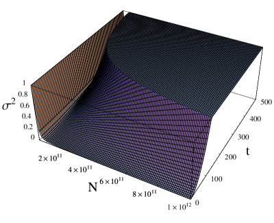
Figure 2: The dependence of the relative fluctuations on the measurement time and the number of photons.

From (46), one can find the optimal number of photons, i.e. the point, where $\sigma^{2}(t)$ reaches minimum in $N$:

$$N_{\text{opt}}=\frac{1}{2g^{2}s_{m}}\sim\frac{4.8\times 10^{12}(\text{sec})}{t},\qquad\sigma^{2}(N_{\text{opt}})=\frac{s_{m}}{4\varphi_{m}^{2}}<1.$$

Consequently, for $h\sim 10^{-22}$, we find the maximum measurement duration:

$$t_{\text{max}}=\frac{16f_{m}^{2}}{\Omega\omega_{gr}^{2}}\approx 1200\text{ sec},$$

as represented in Fig. 3.

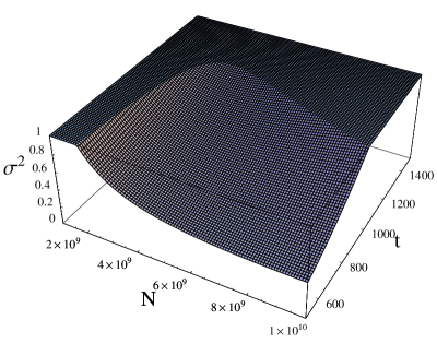
Figure 3: The bounds for the maximum measurement time.

Taking the time of measurement be equal to several periods of the gravitational wave $t\sim 0.01\text{ sec}$, we obtain the following approximate expressions for the functions $\varphi_{t}$, $c_{t}$ and $s_{t}$:

$$|\varphi_{t}|\approx\frac{f_{m}t^{2}\Omega}{2\omega_{gr}},\quad c_{t}\approx\frac{t^{2}}{2},\quad|s_{t}|\approx\frac{t^{3}\Omega}{6}.$$ (47)

In Figs. 4 and 5, we present the dependence of the minimal detectable fluctuations of metric with regard to the time of measurement and the bounds on the laser power which follow from the restriction $\sigma^{2}\leq 1$.

Figure 4: The minimal detectable metric fluctuation.

Figure 5: The limitation on the laser power.

5 Conclusion

Let us summarize briefly the main results of our study. First, formulas (31), (32) and (38), (39) give explicit expressions for the signal and its variance on the output of a two-arm interferometer measuring small classical forces. These formulas take into account full quantum description of system dynamics and irreversible transfer of the system energy to the environment at zero temperature. We point out a fast decrease of the signal and the convergence of its variance to a constant, so that the relative fluctuations tend to infinity (40). Moreover, as it follows from (46), the main quantum noises appear as leading terms in the expansion of the relative fluctuations with respect to the small coupling constant $g^{2}$; they are (i) the Poisson fluctuations of the number of photons (the shot noise), (ii) the standard quantum limit uncertainty relation (due to CCR), (iii) quantum coupling between the oscillator and the laser radiation (the light pressure).

Explicitly calculated density matrix (2) of the system (the radiation $\otimes$ the oscillator) allows one to find the mean values of observables and their variances for arbitrary initial states of the system (e.g. squeezed states).

The study of the oscillator interacting with the electromagnetic radiation, a classical force and the environment at nonzero temperature described by the generator (3) is a more difficult but quite relevant problem. Our approach will be presented in the future paper [16].

The author acknowledges Prof. V.P. Mitrofanov for his helpful discussions.

References

• [1] H. J. Carmichael, An open system approach to quantum optics, Springer, Berlin, 1993.
• [2] G. Lindblad, On generators of quantum dynamical semigroups, Commun. Math. Phys. 48 (1976), 119–130.
• [3] C.W. Gardiner, P. Zoller, Quantum Noise, Springer, 2004.
• [4] C. W. Gardiner and M. J. Collett, Input and output in damped quantum systms: Quantum stochastic differential equations and the master equation, Phys. Rev. A 31 (1985) , 3761-3774.
• [5] B.-G. Englert and G. Morigi, Five Lectures On Dissipative Master Equations, Coherent Evolution in Noisy Environments (Dresden, 2001), Lecture Notes in Physics 611 (2002), 55–106.
• [6] A. M. Chebotarev, A. V. Churkin, G. V. Ryzhakov, A. M. Sinev, A Solvable Model of Gravitational Wave Detector and the Standard Quantum Limit, Russian Journal of Mathematical Physics, V 10, 2 (2003), 134-141.
• [7] Vladimir B. Braginsky, Mikhail L. Gorodetsky, Farid Ya. Khalili, Andrey B. Matsko, Kip S. Thorne, Sergey P. Vyatchanin, The noise in gravitational-wave detectors and other classical-force measurements is not influenced by test-mass quantization, Phys.Rev. D 67 (2003) 082001.
• [8] V.B. Braginsky, Gravitational-wave astronomy: new measurement methods [in Russian], UFN, v.170, 7 (2002), 743-752.
• [9] S. Bose, K. Jacobs and P. L. Knight, Preparation of nonclassical states in cavities with a moving mirror, Phys. Rev. A 56 (1997), 4175–4186 .
• [10] C. Brif and A. Mann, Quantum statistical properties of the radiation field in a cavity with a movable mirror, J.Opt.B Quant.Semiclass.Opt. 2 (2000), 53–61.
• [11] A. M. Chebotarev, Lectures on Quantum Probability, México: Sociedad Matemática Mexicana, Aportaciones Matemáticas. V. 14, 2000.
• [12] H.P. McKean, Stochastic integrals, M.: Mir, 1972.
• [13] I.V. Girsanov, On transforming a certain class of stochastic processes by absolutely continuous substitution of measures [in Russian], Teor. Veroyatnost. i Primenen., 5 : 3 (1960), 314–330.
• [14] Hermann A. Haus, Electromagnetic Noise and Quantum Optical Measurements, Springer, 2000, Ch. 14.
• [15] LSC, Detector Description and Performance for the First Coincidence Observation between LIGO and GEO, Nucl. Instrum. Meth., A 512 (2004) 154–179, or e-print: gr-gc/0308043.
• [16] A.M. Sinev, Quantum trajectories of an oscillator interacting with a heat bath, the coherent light and a weak external force, to be published.